
Wetland Vegetation Classification through Multi-Dimensional Feature Time Series Remote Sensing Images Using Mahalanobis Distance-Based Dynamic Time Warping


Abstract
:1. Introduction
2. Materials and Methods
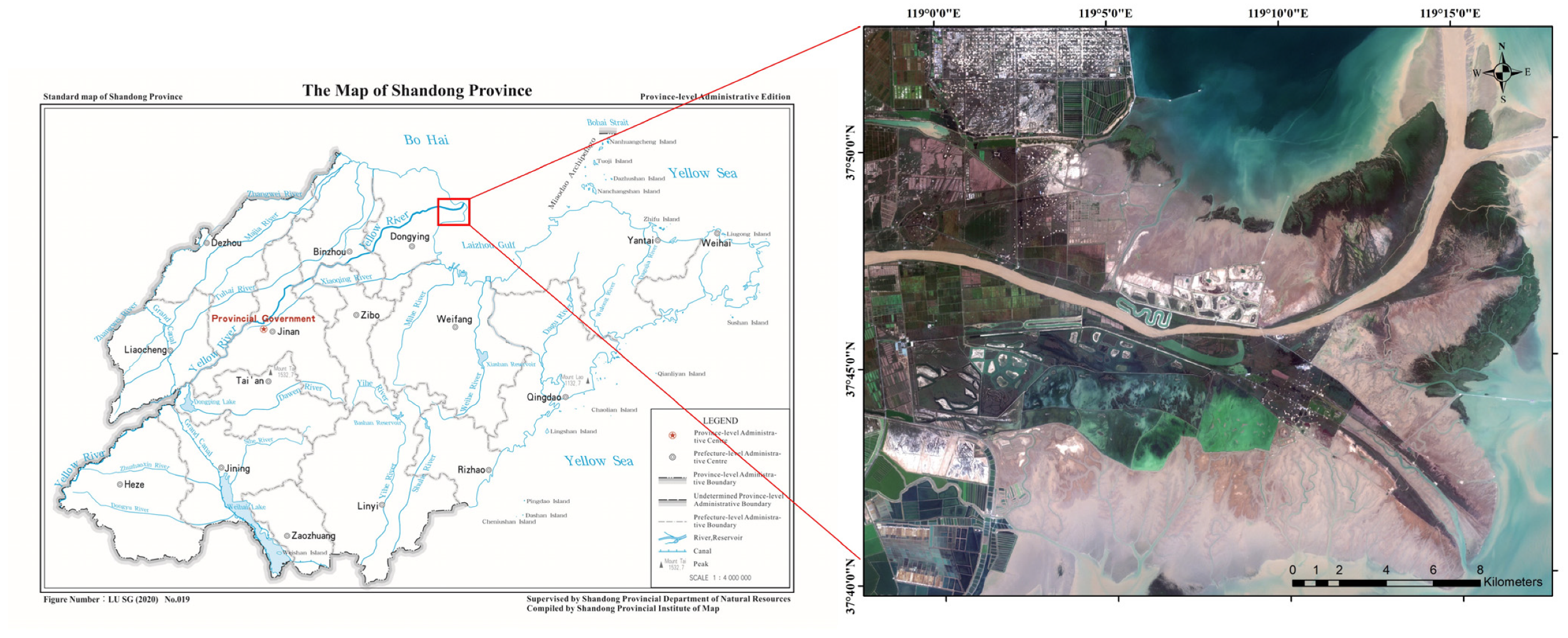
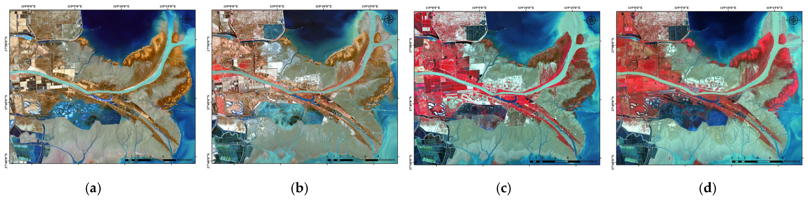
2.1. Study Area
2.2. Data Set
2.2.1. Remote Sensing Data
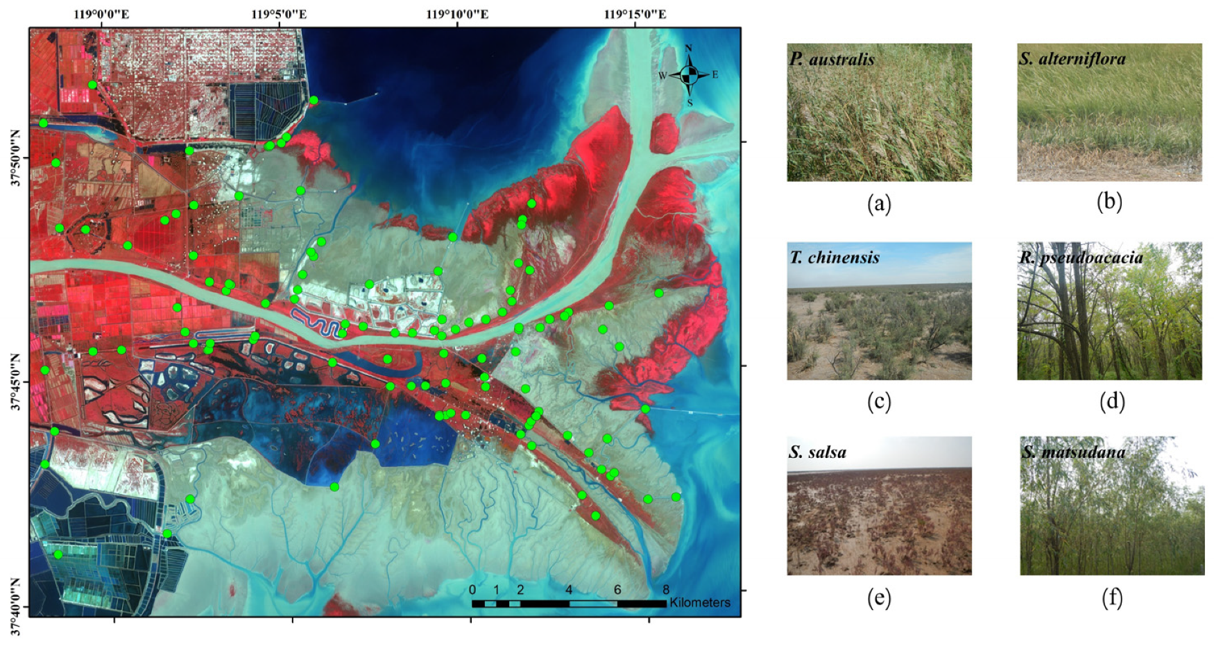
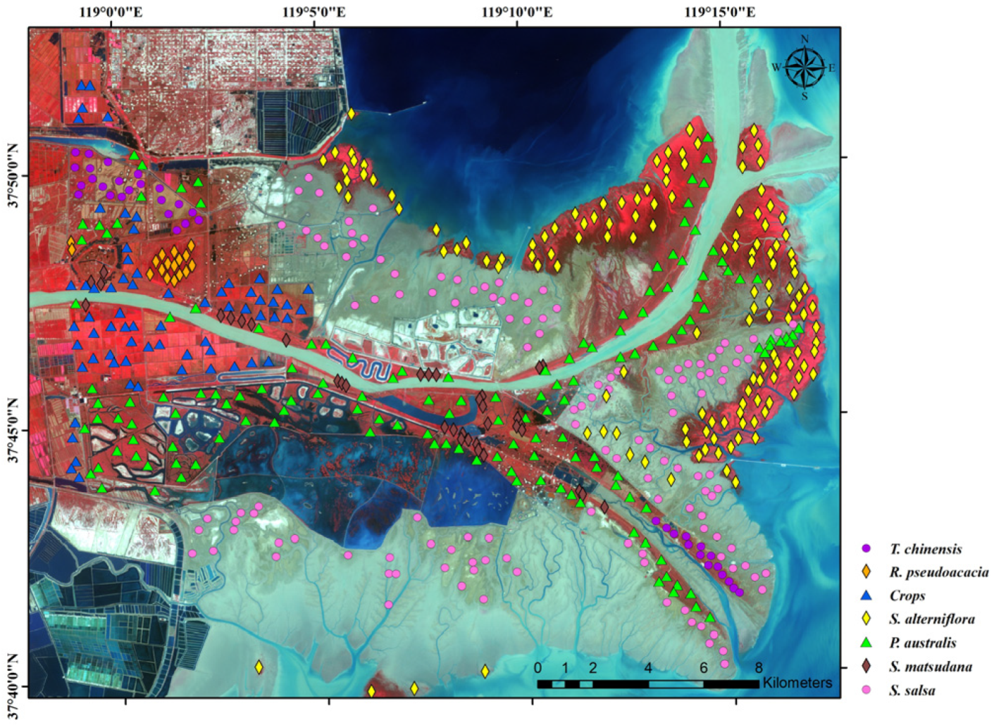
2.2.2. Field Survey Data
2.3. Data Preprocessing
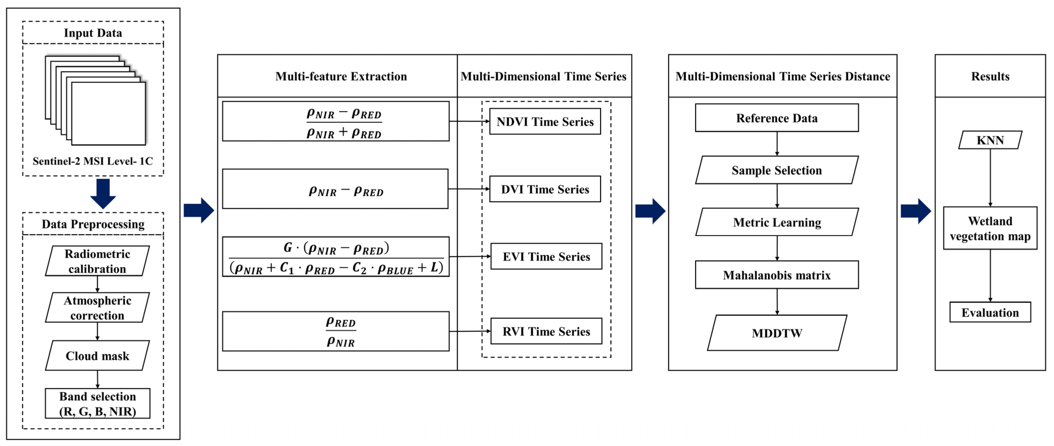
2.4. Methods
2.4.1. Multi-Dimensional Feature Time Series
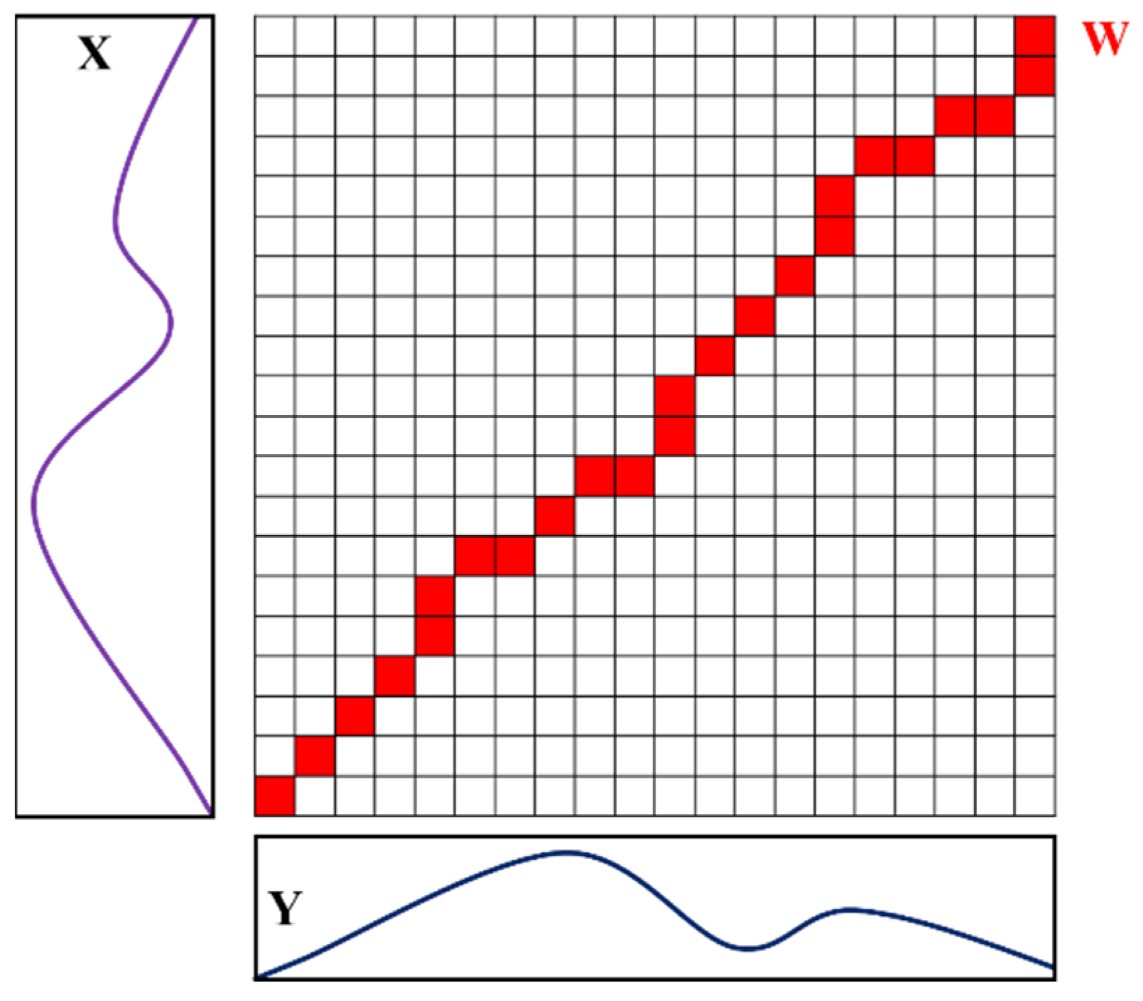
2.4.2. Mahalanobis Distance-Based DTW (MDDTW)
2.4.3. Metric Learning for MDDTW
3. Experiment and Results
3.1. Experiment
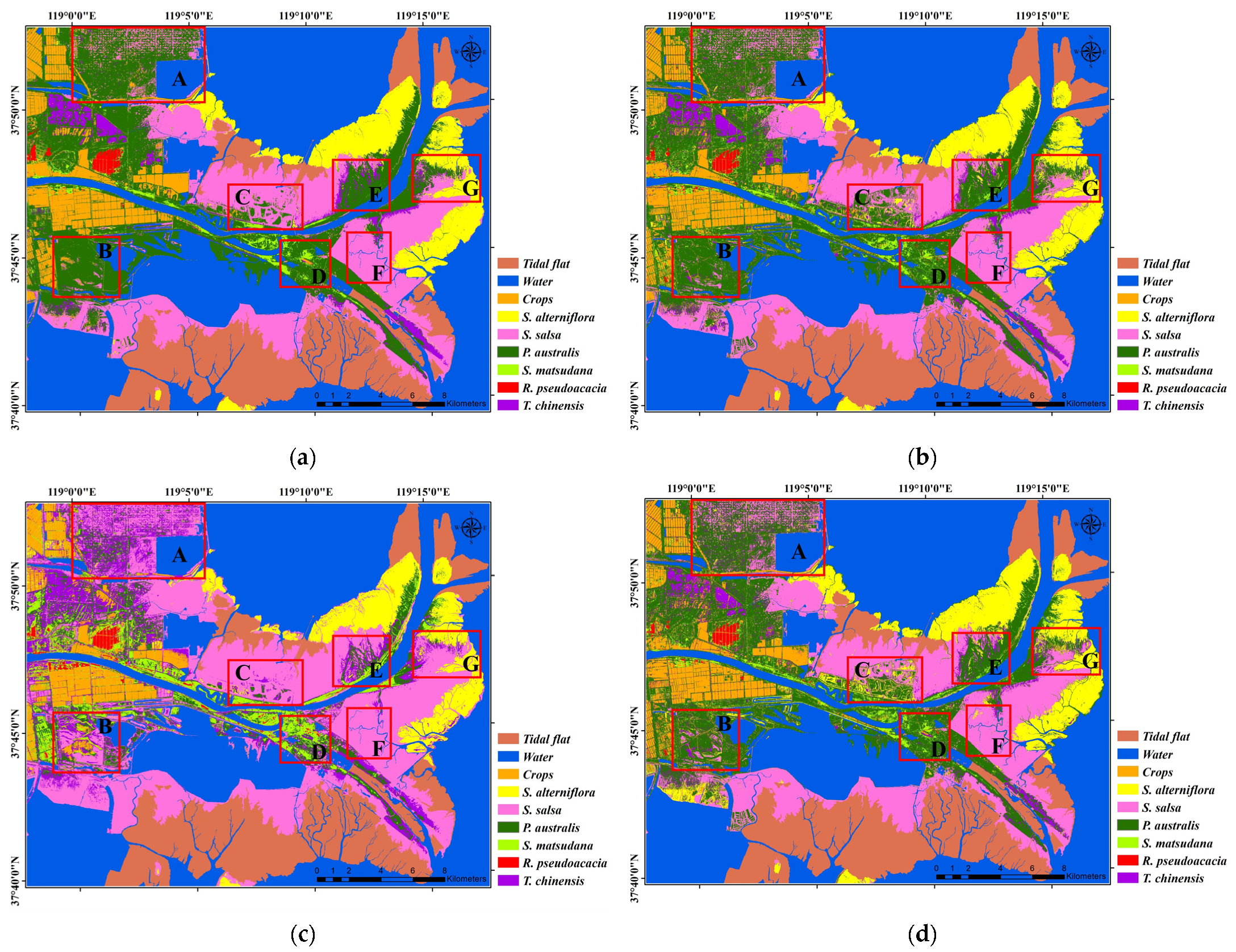
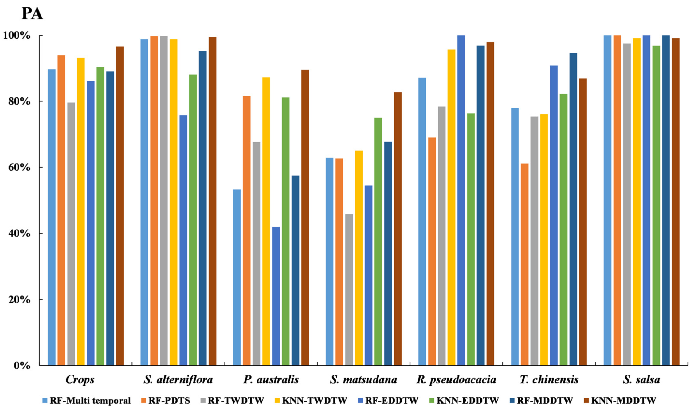
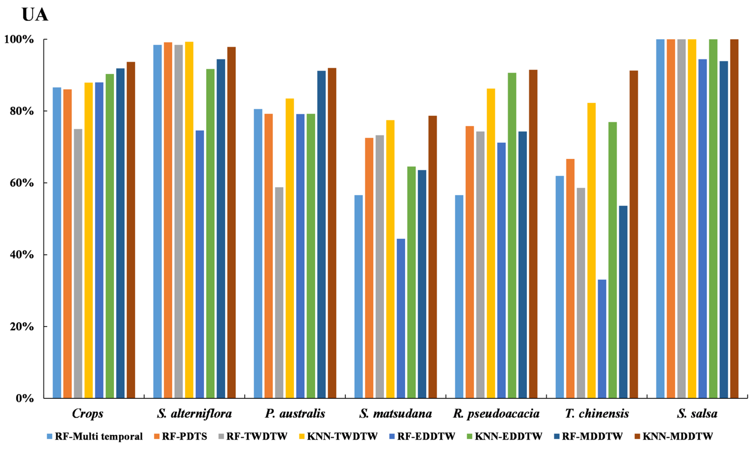
3.2. Result
4. Discussion
4.1. Comparison of Vegetation Classification Methods
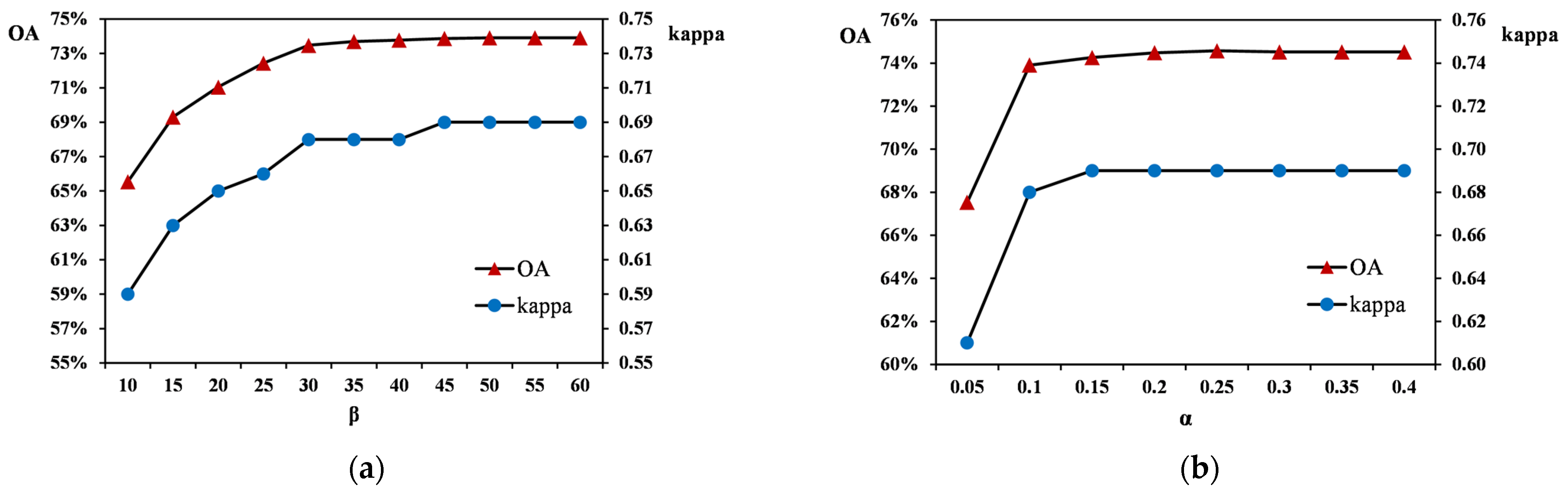
4.2. Influence of Parameters on MDDTW Performance
5. Conclusions
Author Contributions
Funding
Data Availability Statement
Acknowledgments
Conflicts of Interest
Appendix A

| Acronym | Meaning |
|---|---|
| YRD | Yellow River Delta |
| DTW | Dynamic Time Warping |
| MDDTW | Mahalanobis Distance-based Dynamic Time Warping |
| KNN | K-Nearest Neighbors |
| NDVI | Normalized Difference Vegetation Index |
| EVI | Enhanced Vegetation Index |
| RF-PDTS | Random Forest based on pixel-differential time series |
| RF-Multitemporal | Random Forest based on multitemporal |
| TWDTW | Time-Weighted Dynamic Time Warping |
| EDDTW | DTW based on Euclidean distance |
| DVI | Difference Vegetation Index |
| RVI | Ratio Vegetation Index |
References
- Hempattarasuwan, N.; Christakos, G.; Wu, J. Changes of Wiang Nong Lom and Nong Luang wetlands in Chiang Saen Valley (Chiang Rai Province, Thailand) during the period 1988–2017. IEEE J. Sel. Top. Appl. Earth Obs. Remote Sens. 2019, 12, 4224–4238. [Google Scholar] [CrossRef]
- Wang, Y.; Feng, J.; Lin, Q.; Lyu, X.; Wang, X.; Wang, G. Effects of crude oil contamination on soil physical and chemical properties in Momoge wetland of China. Chin. Geogr. Sci. 2013, 23, 708–715. [Google Scholar] [CrossRef]
- Kumar, T.; Mandal, A.; Dutta, D.; Nagaraja, R.; Dadhwal, V.K. Discrimination and classification of mangrove forests using EO-1 Hyperion data: A case study of Indian Sundarbans. Geocarto Int. 2019, 34, 415–442. [Google Scholar] [CrossRef]
- Feddema, J.J.; Oleson, K.W.; Bonan, G.B.; Mearns, L.O.; Buja, L.E.; Meehl, G.A.; Washington, W.M. The importance of land-cover change in simulating future climates. Science 2005, 310, 1674–1678. [Google Scholar] [CrossRef] [Green Version]
- Gallant, A.L. The challenges of remote monitoring of wetlands. Remote Sens. 2015, 7, 10938–10950. [Google Scholar] [CrossRef] [Green Version]
- Zhao, G.; Ye, S.; Gao, M.; Ding, X.; Yuan, H.; Wang, J. Change analysis on eco-environment of the estuary wetland reserve area of Yellow River Delta based on RS and GIS. In Proceedings of the 19th International Conference on Geoinformatics, Shanghai, China, 24–26 June 2011; pp. 1–4. [Google Scholar]
- Cabezas, J.; Galleguillos, M.; Perez-Quezada, J.F. Predicting vascular plant richness in a heterogeneous wetland using spectral and textural features and a random forest algorithm. IEEE Geosci. Remote Sens. Lett. 2016, 13, 646–650. [Google Scholar] [CrossRef]
- Dang, A.T.N.; Kumar, L.; Reid, M.; Nguyen, H. Remote sensing approach for monitoring coastal wetland in the Mekong Delta, Vietnam: Change trends and their driving forces. Remote Sens. 2021, 13, 3359. [Google Scholar] [CrossRef]
- Desclee, B.; Simonetti, D.; Mayaux, P.; Achard, F. Multi-sensor monitoring system for forest cover change assessment in central Africa. IEEE J. Sel. Top. Appl. Earth Obs. Remote Sens. 2013, 6, 110–120. [Google Scholar] [CrossRef]
- Liu, T.; Zhang, X.; Gu, Y. Unsupervised cross-temporal classification of hyperspectral images with multiple geodesic flow kernel learning. IEEE Trans. Geosci. Remote Sens. 2019, 57, 9688–9701. [Google Scholar] [CrossRef]
- Soares, A.; Korting, T.; Fonseca, L.; Bendini, H. Simple nonlinear iterative temporal clustering. IEEE Trans. Geosci. Remote Sens. 2021, 59, 7669–7679. [Google Scholar] [CrossRef]
- Montgomery, J.; Mahoney, C.; Brisco, B.; Boychuk, L.; Cobbaert, D.; Hopkinson, C. Remote sensing of wetlands in the prairie pothole region of North America. Remote Sens. 2021, 13, 3878. [Google Scholar] [CrossRef]
- Leonairo Pencue-Fierro, E.; Solano-Correa, Y.T.; Carlos Corrales-Munoz, J.; Figueroa-Casas, A. A semi-supervised hybrid approach for multitemporal multi-region multisensor Landsat data classification. IEEE J. Sel. Top. Appl. Earth Obs. Remote Sens. 2016, 9, 5424–5435. [Google Scholar] [CrossRef]
- Li, X.; Shen, H.; Zhang, L.; Zhang, H.; Yuan, Q.; Yang, G. Recovering quantitative remote sensing products contaminated by thick clouds and shadows using multitemporal dictionary learning. IEEE Trans. Geosci. Remote Sens. 2014, 52, 7086–7098. [Google Scholar]
- Gao, J.; Yi, Y.; Wei, T.; Zhang, H. Sentinel-2 cloud removal considering ground changes by fusing multitemporal SAR and optical images. Remote Sens. 2021, 13, 3998. [Google Scholar] [CrossRef]
- Melaas, E.K.; Friedl, M.A.; Zhu, Z. Detecting interannual variation in deciduous broadleaf forest phenology using Landsat TM/ETM plus data. Remote Sens. Environ. 2013, 132, 176–185. [Google Scholar] [CrossRef]
- Gomez, C.; White, J.C.; Wulder, M.A. Optical remotely sensed time series data for land cover classification: A review. ISPRS J. Photogramm. Remote Sens. 2016, 116, 55–72. [Google Scholar] [CrossRef] [Green Version]
- Wozniak, E.; Kofman, W.; Aleksandrowicz, S.; Rybicki, M.; Lewinski, S. Multi-temporal indices derived from time series of Sentinel-1 images as a phenological description of plants growing for crop classification. In Proceedings of the 10th International Workshop on the Analysis of Multitemporal Remote Sensing Images (MULTITEMP), Shanghai, China, 5–7 August 2019; pp. 1–4. [Google Scholar]
- Evans, J.P.; Geerken, R. Classifying rangeland vegetation type and coverage using a Fourier component based similarity measure. Remote Sens. Environ. 2006, 105, 1–8. [Google Scholar] [CrossRef]
- Brooks, E.B.; Thomas, V.A.; Wynne, R.H.; Coulston, J.W. Fitting the multitemporal curve: A Fourier series approach to the missing data problem in remote sensing analysis. IEEE Trans. Geosci. Remote Sens. 2012, 50, 3340–3353. [Google Scholar] [CrossRef] [Green Version]
- Du, J.; Shi, J.; Liu, Q.; Jiang, L. Refinement of microwave vegetation index using Fourier analysis for monitoring vegetation dynamics. IEEE Geosci. Remote Sens. Lett. 2013, 10, 1205–1208. [Google Scholar] [CrossRef]
- Chen, J.; Rao, Y.; Shen, M.; Wang, C.; Zhou, Y.; Ma, L.; Tang, Y.; Yang, X. A simple method for detecting phenological change from time series of vegetation index. IEEE Trans. Geosci. Remote Sens. 2016, 54, 3436–3449. [Google Scholar] [CrossRef]
- Zhong, L.; Hu, L.; Yu, L.; Gong, P.; Biging, G.S. Automated mapping of soybean and corn using phenology. ISPRS J. Photogramm. Remote Sens. 2016, 119, 151–164. [Google Scholar] [CrossRef] [Green Version]
- Granero-Belinchon, C.; Adeline, K.; Lemonsu, A.; Briottet, X. Phenological dynamics characterization of alignment trees with Sentinel-2 imagery: A vegetation indices time series reconstruction methodology adapted to urban areas. Remote Sens. 2020, 12, 639. [Google Scholar] [CrossRef] [Green Version]
- Sun, C.; Li, J.; Liu, Y.; Liu, Y.; Liu, R. Plant species classification in salt marshes using phenological parameters derived from Sentinel-2 pixel-differential time-series. Remote Sens. Environ. 2021, 256, 112320. [Google Scholar] [CrossRef]
- Zurita-Milla, R.; Van Gijsel, J.A.E.; Hamm, N.A.; Augustijn, P.W.M.; Vrieling, A. Exploring spatiotemporal phenological patterns and trajectories using self-organizing maps. IEEE Trans. Geosci. Remote Sens. 2013, 51, 1914–1921. [Google Scholar] [CrossRef]
- Lee, B.; Kim, E.; Lim, J.; Seo, B.; Chung, J. Detecting vegetation phenology in various forest types using long-term MODIS vegetation indices. In Proceedings of the 2018 IEEE International Geoscience and Remote Sensing Symposium (IGARSS), Valencia, Spain, 23–27 July 2018; pp. 5243–5246. [Google Scholar]
- Ghaderpour, E.; Vujadinovic, T. Change detection within remotely sensed satellite image time series via spectral analysis. Remote Sens. 2020, 12, 4001. [Google Scholar] [CrossRef]
- Petitjean, F.; Inglada, J.; Gancarski, P. Satellite image time series analysis under time warping. IEEE Trans. Geosci. Remote Sens. 2012, 50, 3081–3095. [Google Scholar] [CrossRef]
- Jiang, Y.; Qi, Y.; Wang, W.K.; Bent, B.; Avram, R.; Olgin, J.; Dunn, J. EventDTW: An improved dynamic time warping algorithm for aligning biomedical signals of nonuniform sampling frequencies. Sensors 2020, 20, 2700. [Google Scholar] [CrossRef]
- Guan, X.; Huang, C.; Liu, G.; Meng, X.; Liu, Q. Mapping rice cropping systems in Vietnam using an NDVI-based time-series similarity measurement based on DTW distance. Remote Sens. 2016, 8, 19. [Google Scholar] [CrossRef] [Green Version]
- Maus, V.; Camara, G.; Cartaxo, R.; Sanchez, A.; Ramos, F.M.; de Queiroz, G.R. A time-weighted dynamic time warping method for land-use and land-cover mapping. IEEE J. Sel. Top. Appl. Earth Obs. Remote Sens. 2016, 9, 3729–3739. [Google Scholar] [CrossRef]
- Belgiu, M.; Csillik, O. Sentinel-2 cropland mapping using pixel-based and object-based time-weighted dynamic time warping analysis. Remote Sens. Environ. 2018, 204, 509–523. [Google Scholar] [CrossRef]
- Zhao, F.; Yang, G.; Yang, X.; Cen, H.; Zhu, Y.; Han, S.; Yang, H.; He, Y.; Zhao, C. Determination of key phenological phases of winter wheat based on the time-weighted dynamic time warping algorithm and MODIS time-series data. Remote Sens. 2021, 13, 1836. [Google Scholar] [CrossRef]
- Hao, P.; Wang, L.; Zhan, Y.; Niu, Z.; Wu, M. Using historical NDVI time series to classify crops at 30 m spatial resolution: A case in Southeast Kansas. In Proceedings of the 2016 IEEE International Geoscience and Remote Sensing Symposium (IGARSS), Beijing, China, 10–15 July 2016; pp. 6316–6319. [Google Scholar]
- Huang, Y.; Liu, X.; Li, X.; Yan, Y.; Ou, J. Comparing the effects of temporal features derived from synthetic time-series NDVI on fine land cover classification. IEEE J. Sel. Top. Appl. Earth Obs. Remote Sens. 2018, 11, 4618–4629. [Google Scholar] [CrossRef]
- Csillik, O.; Belgiu, M.; Asner, G.P.; Kelly, M. Object-based time-constrained dynamic time warping classification of crops using Sentinel-2. Remote Sens. 2019, 11, 1257. [Google Scholar] [CrossRef] [Green Version]
- Lewandowski, M.; Makris, D.; Velastin, S.A.; Nebel, J.C. Structural laplacian eigenmaps for modeling sets of multivariate sequences. IEEE Trans. Cybern. 2014, 44, 936–949. [Google Scholar] [CrossRef] [PubMed]
- Gupta, A.; Gupta, H.P.; Biswas, B.; Dutta, T. Approaches and applications of early classification of time series: A review. IEEE Trans. Artif. Intell. 2020, 1, 47–61. [Google Scholar] [CrossRef]
- Weng, X.; Shen, J. Classification of multivariate time series using two-dimensional singular value decomposition. Knowl.-Based Syst. 2008, 21, 535–539. [Google Scholar] [CrossRef]
- Liu, C.; Tao, R.; Li, W.; Zhang, M.; Sun, W.; Du, Q. Joint classification of hyperspectral and multispectral images for mapping coastal wetlands. IEEE J. Sel. Top. Appl. Earth Obs. Remote Sens. 2021, 14, 982–996. [Google Scholar] [CrossRef]
- Louis, J.; Pflug, B.; Main-Knorn, M.; Debaecker, V.; Mueller-Wilm, U.; Iannone, R.Q.; Cadau, E.G.; Boccia, V.; Gascon, F. Sentinel-2 global surface reflectance level-2a product generated with Sen2cor. In Proceedings of the 2019 IEEE International Geoscience and Remote Sensing Symposium (IGARSS), Yokohama, Japan, 28 July–2 August 2019; pp. 8522–8525. [Google Scholar]
- Qiu, S.; Zhu, Z.; He, B. Fmask 4.0: Improved cloud and cloud shadow detection in Landsats 4–8 and Sentinel-2 imagery. Remote Sens. Environ. 2019, 231, 111205. [Google Scholar] [CrossRef]
- Jordan, C.F. Derivation of leaf-area index from quality of light on the forest floor. Ecology 1969, 50, 663–666. [Google Scholar] [CrossRef]
- Liu, H.Q.; Huete, A. A feedback based modification of the NDVI to minimize canopy background and atmospheric noise. IEEE Trans. Geosci. Remote Sens. 1995, 33, 457–465. [Google Scholar] [CrossRef]
- Zhu, Y.; Yao, X.; Tian, Y.; Liu, X.; Cao, W. Analysis of common canopy vegetation indices for indicating leaf nitrogen accumulations in wheat and rice. Int. J. Appl. Earth Obs. Geoinf. 2008, 10, 1–10. [Google Scholar] [CrossRef]
- Qian, L.; Zhang-qin, H.; Yi-bin, H.; Rui, C. Utterance verification on DTW based speech recognition using likelihood. In Proceedings of the 2010 International Conference on Computer Application and System Modeling (ICCASM 2010), Taiyuan, China, 22–24 October 2010; Volume 2, pp. 427–431. [Google Scholar]
- Jambhale, S.S.; Khaparde, A. Gesture recognition using DTW & piecewise DTW. In Proceedings of the 2014 21st International Conference on Electronics and Communication Systems (ICECS 2014), Marseille, France, 7–10 December 2014; pp. 1–5. [Google Scholar]
- Lampert, T.; Lafabregue, B.; Gançarski, P. Constrained distance-based clustering for satellite image time-series. IEEE J. Sel. Top. Appl. Earth Obs. Remote Sens. 2019, 12, 4606–4621. [Google Scholar] [CrossRef]
- Wang, X.; Jiang, M.; Chen, S.; Yang, C.; Jing, W.; Guo, Z. A hybrid time series matching algorithm based on feature-points and DTW. In Proceedings of the 2016 9th International Symposium on Computational Intelligence and Design (ISCID 2016), Hangzhou, China, 10–11 December 2016; Volume 2, pp. 171–175. [Google Scholar]
- Zhong, Y.; Lin, X.; Zhang, L. A support vector conditional random fields classifier with a Mahalanobis distance boundary constraint for high spatial resolution remote sensing imagery. IEEE J. Sel. Top. Appl. Earth Obs. Remote Sens. 2014, 7, 1314–1330. [Google Scholar] [CrossRef]
- Shen, C.; Kim, J.; Wang, L. Scalable large-margin Mahalanobis distance metric learning. IEEE Trans. Neural Netw. 2010, 21, 1524–1530. [Google Scholar] [CrossRef] [Green Version]
- Mei, J.; Liu, M.; Karimi, H.R.; Gao, H. LogDet divergence-based metric learning with triplet constraints and its applications. IEEE Trans. Image Process. 2014, 23, 4920–4931. [Google Scholar] [CrossRef] [PubMed]
- Mei, J.; Liu, M.; Wang, Y.F.; Gao, H. Learning a Mahalanobis distance-based dynamic time warping measure for multivariate time series classification. IEEE Trans. Cybern. 2016, 46, 1363–1374. [Google Scholar] [CrossRef] [PubMed]
- Davis, J.V.; Kulis, B.; Jain, P.; Sra, S.; Dhillon, I.S. Information-theoretic metric learning. Machine Learning. In Proceedings of the Twenty-Fourth International Conference (ICML 2007), Corvallis, OR, USA, 20–24 June 2007; pp. 209–216. [Google Scholar]
- Jain, P.; Kulis, B.; Dhillon, I.S.; Grauman, K. Online metric learning and fast similarity search. Advances in Neural Information Processing Systems 21. In Proceedings of the Twenty-Second Annual Conference on Neural Information Processing Systems, Vancouver, BC, Canada, 8–11 December 2008; pp. 761–768. [Google Scholar]
- Bernhard, S.; John, P.; Thomas, H. Differential Entropic Clustering of Multivariate Gaussians. In Advances in Neural Information Processing Systems 19: Proceedings of the 2006 Conference; MIT Press: Cambridge, MA, USA, 2007; pp. 337–344. [Google Scholar]
- Orsenigo, C.; Vercellis, C. Combining discrete SVM and fixed cardinality warping distances for multivariate time series classification. Pattern Recogn. 2010, 43, 3787–3794. [Google Scholar] [CrossRef]
- Gravano, L.; Paparrizos, J. K-shape: Efficient and accurate clustering of time series. In Proceedings of the 2015 ACM SIGMOD International Conference on Management of Data, Melbourne, Victoria, Australia, 27 May 2015; Volume 45, pp. 69–76. [Google Scholar]
- Qu, C.; Li, P. Winter wheat mapping from Landsat NDVI time series data using time-weighted dynamic time warping and phenological rules. In Proceedings of the 2020 IEEE International Geoscience and Remote Sensing Symposium (IGARSS), Waikoloa, HI, USA, 26 September–2 October 2020; pp. 4183–4186. [Google Scholar]


| Satellite Name | Sentinel-2 Sensing Date in 2019 | ||||||||
|---|---|---|---|---|---|---|---|---|---|
| Sentinel-2A | 02/21 | 03/13 | 03/23 | 04/02 | 05/02 | 05/12 | 05/22 | 06/11 | 07/01 |
| 07/21 | 09/09 | 09/29 | 10/19 | 10/29 | 11/08 | 11/28 | 12/08 | 12/28 | |
| Sentinel-2B | 01/17 | 02/16 | 03/08 | 04/07 | 04/17 | 05/07 | 05/27 | 06/26 | 07/26 |
| 08/15 | 08/25 | 09/24 | 12/03 | ||||||
| Classification Type | OA (%) | Kappa |
|---|---|---|
| RF-Multitemporal | 80.63 | 0.77 |
| RF-PDTS | 88.30 | 0.85 |
| RF-TWDTW | 78.58 | 0.75 |
| KNN-TWDTW | 91.25 | 0.89 |
| RF-EDDTW | 70.95 | 0.66 |
| KNN-EDDTW | 86.50 | 0.83 |
| RF-MDDTW | 82.39 | 0.79 |
| KNN-MDDTW | 94.56 | 0.93 |
| Crops | SA | PA | SM | RP | TC | SS | PA | |
|---|---|---|---|---|---|---|---|---|
| Method: RF-PDTS, Overall accuracy = 88.30%, kappa = 0.85 | ||||||||
| Crops | 524 | 0 | 18 | 3 | 2 | 11 | 0 | 93.91% |
| SA | 0 | 1240 | 3 | 0 | 1 | 0 | 0 | 99.68% |
| PA | 40 | 0 | 1022 | 75 | 15 | 100 | 0 | 81.63% |
| SM | 39 | 6 | 76 | 235 | 19 | 0 | 0 | 62.67% |
| RP | 0 | 0 | 51 | 1 | 116 | 0 | 0 | 69.05% |
| TC | 6 | 5 | 120 | 10 | 0 | 222 | 0 | 61.12% |
| SS | 0 | 0 | 0 | 0 | 0 | 0 | 1188 | 100% |
| UA | 86.04% | 99.12% | 79.22% | 72.53% | 75.82% | 66.67% | 100% | |
| Method: KNN-TWDTW, Overall accuracy = 91.25%, kappa = 0.89 | ||||||||
| Crops | 530 | 0 | 29 | 3 | 3 | 4 | 0 | 93.15% |
| SA | 2 | 1242 | 11 | 2 | 0 | 0 | 0 | 98.81% |
| PA | 34 | 5 | 1097 | 67 | 5 | 49 | 0 | 87.27% |
| SM | 12 | 1 | 106 | 251 | 13 | 3 | 0 | 65.03% |
| RP | 4 | 0 | 1 | 1 | 132 | 0 | 0 | 95.65% |
| TC | 18 | 3 | 65 | 0 | 0 | 274 | 0 | 76.11% |
| SS | 3 | 0 | 5 | 0 | 0 | 3 | 1188 | 99.08% |
| UA | 87.89% | 99.28% | 83.49% | 77.47% | 86.27% | 82.28% | 100.00% | |
| Method: KNN-MDDTW, Overall accuracy = 94.56%, kappa = 0.93 | ||||||||
| Crops | 565 | 1 | 18 | 0 | 1 | 0 | 0 | 96.58% |
| SA | 0 | 1224 | 5 | 1 | 0 | 1 | 0 | 99.43% |
| PA | 24 | 23 | 1209 | 66 | 9 | 19 | 0 | 89.56% |
| SM | 4 | 0 | 46 | 255 | 2 | 1 | 0 | 82.79% |
| RP | 1 | 0 | 0 | 2 | 140 | 0 | 0 | 97.90% |
| TC | 9 | 1 | 35 | 0 | 1 | 304 | 0 | 86.86% |
| SS | 0 | 2 | 1 | 0 | 0 | 8 | 1188 | 99.08% |
| UA | 93.70% | 97.84% | 92.01% | 78.70% | 91.50% | 91.29% | 100.00% | |
Publisher’s Note: MDPI stays neutral with regard to jurisdictional claims in published maps and institutional affiliations. |
© 2022 by the authors. Licensee MDPI, Basel, Switzerland. This article is an open access article distributed under the terms and conditions of the Creative Commons Attribution (CC BY) license (https://creativecommons.org/licenses/by/4.0/).
Share and Cite
Li, H.; Wan, J.; Liu, S.; Sheng, H.; Xu, M. Wetland Vegetation Classification through Multi-Dimensional Feature Time Series Remote Sensing Images Using Mahalanobis Distance-Based Dynamic Time Warping. Remote Sens. 2022, 14, 501. https://doi.org/10.3390/rs14030501
Li H, Wan J, Liu S, Sheng H, Xu M. Wetland Vegetation Classification through Multi-Dimensional Feature Time Series Remote Sensing Images Using Mahalanobis Distance-Based Dynamic Time Warping. Remote Sensing. 2022; 14(3):501. https://doi.org/10.3390/rs14030501
Chicago/Turabian StyleLi, Huayu, Jianhua Wan, Shanwei Liu, Hui Sheng, and Mingming Xu. 2022. "Wetland Vegetation Classification through Multi-Dimensional Feature Time Series Remote Sensing Images Using Mahalanobis Distance-Based Dynamic Time Warping" Remote Sensing 14, no. 3: 501. https://doi.org/10.3390/rs14030501