A Method of Vision Aided GNSS Positioning Using Semantic Information in Complex Urban Environment

Abstract

High-precision localization through multi-sensor fusion has become a popular research direction in unmanned driving. However, most previous studies have performed optimally only in open-sky conditions; therefore, high-precision localization in complex urban environments required an urgent solution. The complex urban environments employed in this study include dynamic environments, which result in limited visual localization performance, and highly occluded environments, which yield limited global navigation satellite system (GNSS) performance. In order to provide high-precision localization in these environments, we propose a vision-aided GNSS positioning method using semantic information by integrating stereo cameras and GNSS into a loosely coupled navigation system. To suppress the effect of dynamic objects on visual positioning accuracy, we propose a dynamic-simultaneous localization and mapping (Dynamic-SLAM) algorithm to extract semantic information from images using a deep learning framework. For the GPS-challenged environment, we propose a semantic-based dynamic adaptive Kalman filtering fusion (S-AKF) algorithm to develop vision aided GNSS and achieve stable and high-precision positioning. Experiments were carried out in GNSS-challenged environments using the open-source KITTI dataset to evaluate the performance of the proposed algorithm. The results indicate that the dynamic-SLAM algorithm improved the performance of the visual localization algorithm and effectively suppressed the error spread of the visual localization algorithm. Additionally, after vision was integrated, the loosely-coupled navigation system achieved continuous high-accuracy positioning in GNSS-challenged environments.

1. Introduction

The Global Navigation Satellite System (GNSS) can provide highly reliable, globally valid and highly accurate position information, carrier velocities and precise times [1,2]. It has gradually become the foundation of most positioning and navigation applications, including autonomous driving vehicles (ADVs) [3,4] and guided weapons. As the positioning performance of GNSS depends on the continuous tracking of the passible radio signal, the accuracy, availability, and continuity deteriorate in GNSS-challenged environments [5,6]. Therefore, the low availability is compensated with additional sensors in complex environments like urban canyons or tunnels. Additionally, there is an increasing attractiveness to keeping high-precision positioning for multi-sensor navigation systems when GPS fails due to automobile and UAS crashes.

In the field of combined navigation, most researches were focused on the integration of GNSS and inertial navigation system (INS) [7,8,9,10,11]. With the advances in microelectromechanical system (MEMS) inertial sensor technologies, low-cost GNSS/MEMS-IMU (inertial measurement units) integration can achieve high-accuracy positioning in open-sky environments [12,13,14]. However, the rapid divergence of estimation errors in the low-cost MEMS-IMU can lead to poor performance in the absence of GPS. Therefore, in this study we attempt to use another low-cost sensor, a stereo camera, to aid GNSS in providing continuous position estimations when GPS signals are not available.

Visual simultaneous localization and mapping (SLAM) is the state-of-the-art solution for high-precision localization using a stereo camera. Visual SLAM solutions are either filter-based [15,16,17], using a Kalman filter, or keyframe-based [18,19], relying on optimization, to estimate both motion and structure. In the first approach, every frame is processed by the filter to jointly estimate the map feature locations and camera pose. However, this approach is computationally expensive when processing consecutive frames, and yields minimal new information and accumulating linearization errors [17]. The latter method is more accurate than filtering for the same computational cost [20]. However, this method also has the drawbacks of unavoidable losses of performance in the presence of excessive dynamic feature points. In this study, we proposed a dynamic-SLAM algorithm to optimize the keyframe-based visual SLAM solution by semantic segmentation.

GNSS and visual SLAM offer complementary properties, which make them particularly suitable for fusion. To perform sensor fusion, [21] focus on the online GPS-aided visual inertial odometry (GPS-VIO) spatiotemporal sensor calibration and frame initialization. GPS position measurements were fused with VIO estimates using an optimization-based tightly coupled approach in [22]. However, the propagation step is driven by high frequency inertial measurements, making the IMU an indispensable sensor. In [23,24], the authors propose a decoupled Graph-Optimization based Multi-Sensor Fusion approach (GOMSF), which solve the real-time alignment problem between the local base frame of VIO and the global base frame of GNSS. In [25,26,27], an Extended Kalman Filter (EKF) is proposed to fuse GPS data and a camera-based pose estimate and obtain drift-free pose estimates, allowing a Micro Aerial Vehicle (MAV) state prediction at 1 kHz for accurate control. Though all of these works report satisfactory results, the optimization-based approach is lack of discussing the potential for GPS failures, and the filter-based approach did not take advantage of the semantic information of images. In [28,29,30], the integration of a camera, INS and GNSS allows the GNSS to maintain positioning accuracy in a GNSS-challenged environment. In [31], the authors incorporated carrier phase differential GPS measurements into the bundle-adjustment based visual SLAM framework to obtain high-precision globally referenced positions and velocities. In [32], the authors integrate GPS, IMU, wheel odometry, and LIDAR data to generate high-resolution environment maps, which can significantly improve the localization accuracy and availability. However, the changes on road surfaces will easily cause the environment maps invalid and performance degradation. In this study, we proposed a loosely-coupled GNSS/Vision integration system using a S-AKF algorithm.

Previous multi-sensor fusion research has mostly focused on the fusion of GNSS, IMU and camera, and most related algorithms are only effective in an open-sky environment. Instead of a tightly coupled GNSS/IMU/Vision navigation, which may need a lot of effort to align all other, potentially delayed, sensor readings with states, a loosely-coupled navigation can obtain a similar positioning performance without an IMU. In this contribution, we take advantages of the rich information provided by stereo cameras, employ semantic information to provide more effective constraints for the fusion of multiple sensors, and adopt a loosely-coupled integrated system to avoid excessive computational consumption. In summary, we proposed a method of vision aided GNSS positioning to achieve continuous high-precision positioning when occurring GPS failures. In order to verify the performance of the method, we used the open-source KITTI dataset to conduct the experiments.

The remainder of this paper is organized as follows. Section 2 introduces the improved visual slam algorithm, GNSS measurement model, improved adaptive Kalman filter algorithm, and loosely coupled vision and GNSS model for GNSS-challenged environments. Section 3 introduced the experimental data collection environment and presents the experimental results. Finally, Section 5 analyze the performance of the algorithm based on the experimental results and draw the corresponding conclusions and prospects.

2. Methods

Loosely coupled navigation systems are suitable multi-sensor fusion approaches for vision sensors and GNSS. In this study, to enable assistance between vision sensors and GNSS for high-accuracy positioning, we first optimized the vision positioning algorithm to maintain stable and optimal positioning performance in dynamic environments. The following subsections introduce the optimized visual SLAM model, double-difference measurement model, dynamic adaptive Kalman filtering algorithm-based semantic, and loosely coupled RTK/Vision integration system model.

2.1. Visual SLAM Model

To solve the problems associated with inadequate performance of the visual slam algorithm in a dynamic environment, we used a semantic segmentation framework to reduce the impact of dynamic objects on pose estimation. The processing framework of the visual positioning algorithm (Dynamic-SLAM) is shown in Figure 1. Dynamic-SLAM was optimized based on ORB-SLAM2 [33], which is currently the most advanced keyframe-based visual slam algorithm available. Visual odometry (VO), which obtained the real-time camera pose tracking based on the transformation between frames, is the front end of visual SLAM. We added a real-time semantic segmentation thread in the VO module to reduce the influence of dynamic objects on pose estimation. The image frames were transmitted to the tracking thread and the YOLO thread. The tracking thread extract features from frames and obtains a feature image containing features on dynamic objects and features on static objects. The YOLO thread segments the semantic from frames and obtains a mask image with semantic labels. Then, we can remove all the outliers on dynamic objects by merging the feature image and mask image. Without the effect of dynamic objects, both the robustness of the algorithm and the positioning accuracy were improved.

Figure 2 shows the pipeline of our loosely-coupled GNSS/Vision integration system. Consecutive images, which are the input of VO, were processed by the feature extraction pipeline and deep learning segmentation network. After the semantic segmentation, feature points on dynamic objects were labeled as outliers. The segmentation category labels help the feature points weighting and rich descriptor computation. The classified feature points were computed by point-wise matching with the previous frame. Then, the inlier points were calculated by minimizing reprojection error to estimate camera pose translation.

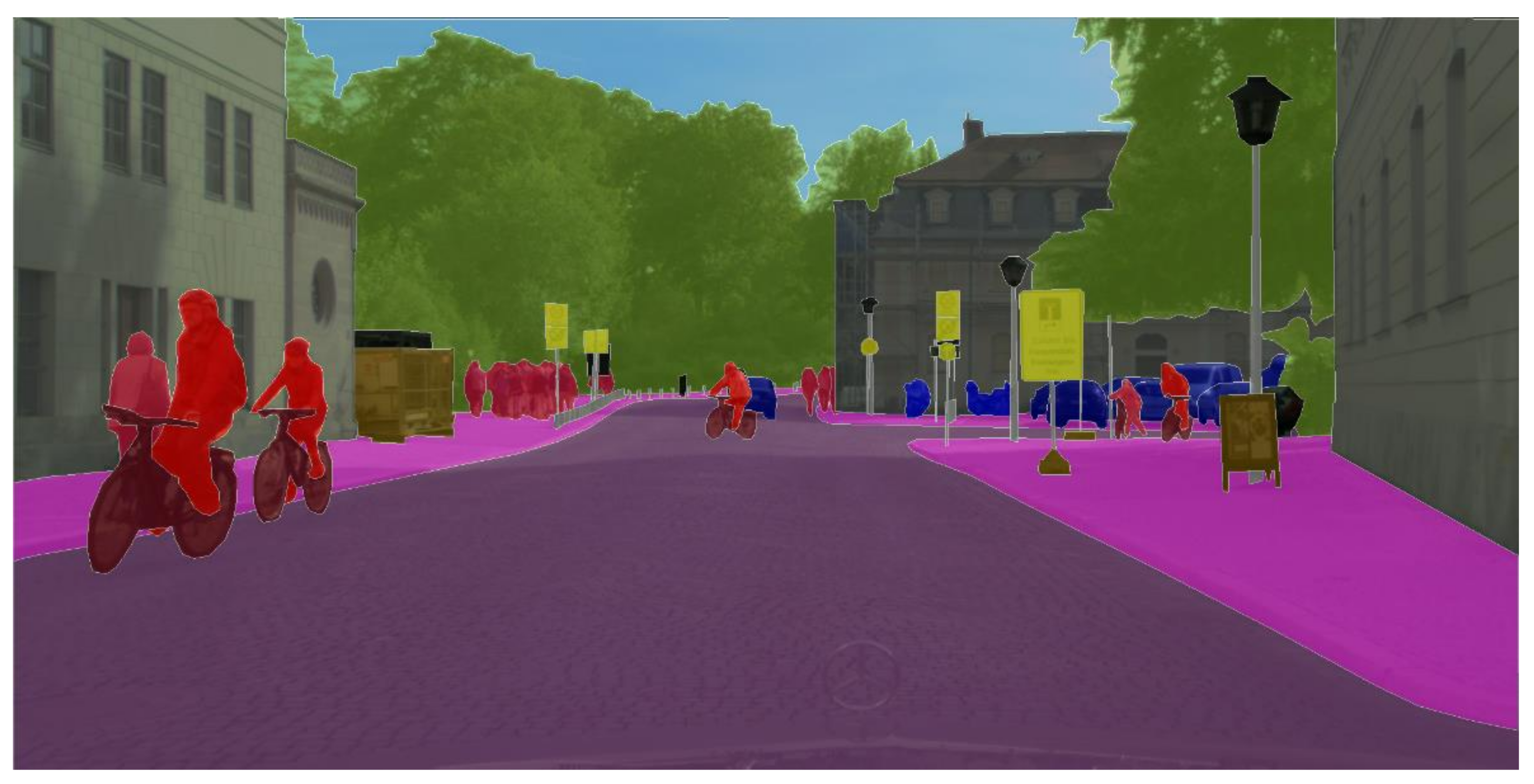
Dynamic-SLAM can segment dynamic objects in the environment. As shown in Figure 3, both cars and bicycles were identified and marked with different colors. Furthermore, Dynamic-SLAM can identify obstructing objects in the environment, such as tree shade and tall buildings. Dynamic-SLAM can obtain depth information of the surrounding environment by a local mapping thread, which denotes the position in Z direction under the world coordinate system. Using the depth information of obstructing objects, the corresponding occlusion factor k can be calculated, which aids in the subsequent adaptive adjustments to the Kalman filter weight. The occlusion factor k can be formulated as follows:

$$\mathrm{k}=1.5{\log }_{10}\left(\mathrm{d}\right)-1$$

(1)

where d denotes the depth of obstructing objects.

To perform real-time positioning, we have to strike a balance between real-time and accuracy. Our visual positioning algorithm uses the YOLOv5 (You Only Look Once version 5) algorithm based on the Darknet deep learning framework to provide pixel-wise real-time semantic segmentation. We use the Cityscapes dataset for training, and the resulting model segmented a total of 34 classes. In outdoor scenes, we recognize pedestrians and vehicles as dynamic objects, and denoted the feature points on dynamic objects as outliers.

2.2. Double-Differenced Measurement Model

GPS basic observation mainly includes pseudorange observation and carrier phase observation. The pseudo-range is obtained by measuring the propagation time of the satellite signal from the satellite to the receiver and multiplying it by the speed of light. Carrier phase is the phase difference between the carrier signal received by the receiver and the carrier signal generated by the receiver. According to the definition of the pseudorange and phase observables, their localization equations can be written as:

$${\mathrm{L}}_{\mathrm{C}}=\mathit{A}\delta \mathit{x}+\mathrm{c}\delta {\mathrm{t}}_{\mathrm{r}}+{\mathrm{d}}_{\mathrm{ion}}+{\mathrm{d}}_{\mathrm{trop}}+{\epsilon }_{\rho }$$

(2)

$${\mathrm{L}}_{\phi }=\mathit{A}\delta \mathit{x}-\lambda \mathrm{N}+\mathrm{c}\delta {\mathrm{t}}_{\mathrm{r}}-{\mathrm{d}}_{\mathrm{ion}}+{\mathrm{d}}_{\mathrm{trop}}+{\epsilon }_{\phi }$$

(3)

with

$${\mathrm{L}}_c=\tilde{\rho }-{\rho }^0$$

(4)

$${\mathrm{L}}_{\phi }=\lambda \phi -{\rho }^0$$

(5)

where $\tilde{\rho }$ and $\phi$ denote the pseudorange and carrier phase observations, respectively; $\lambda$ and c are the carrier wavelength and the speed of light in vacuum; ${\rho }^0$ is the approximate geometric distance between satellite and station; $\mathit{A}$ is the linearization coefficient matrix; $\delta \mathit{x}$ denotes the correction of station coordinate; $\delta {\mathrm{t}}_{\mathrm{r}}$ denotes the receiver clock difference; ${\mathrm{d}}_{\mathrm{ion}}$ and ${\mathrm{d}}_{\mathrm{trop}}$ denote ionospheric refraction error and tropospheric refraction error, respectively; ${\epsilon }_{\rho }$ and ${\epsilon }_{\phi }$ denote the unmodeled residual error of the pseudorange and carrier phase observation, respectively.

The accuracy of the pseudorange observation was relatively low, and the use of phase observations for high-precision dynamic positioning requires real-time resolution of the ambiguity parameter, N. For short baseline positioning, the atmospheric errors between stations had a strong correlation, therefore, the synchronous observation difference method between stations was used to eliminate or reduce the influence of these errors.

For two receivers simultaneously observing multiple satellites, the double-difference observation equation can be expressed as follows:

$$\nabla {\Delta \mathrm{L}}_{\mathrm{C}12}^{\mathrm{ij}}=\nabla {\mathit{A}}_2^{ij}\delta {\mathit{x}}_2+\nabla \Delta {\epsilon }_{\rho }$$

(6)

$$\nabla {\Delta \mathrm{L}}_{\phi 12}^{\mathrm{i}j}=\nabla {\mathit{A}}_2^{ij}\delta {\mathit{x}}_2-\lambda \nabla \Delta {\mathit{N}}_{12}^{ij}+\nabla \Delta {\epsilon }_{\phi }$$

(7)

where the superscripts i and j denote the satellite sequence; the subscripts 1 and 2 denote the station number; and $\nabla \Delta \left(\cdot \right)$ denotes the double-differencing operator.

The double-difference observation model eliminates the receiver clock error, reduces the modeling of the receiver clock error, and enables relatively simple data processing. In addition, for carrier-phase double-difference positioning, the elimination of these errors provides favorable conditions for a dynamic solution to the double-difference ambiguity.

2.3. Adaptive Kalman Filter

2.3.1. Kalman Filtering and the Influence of Filtering Parameters

The system model of Kalman filter was constructed as follows:

$$\left\{\begin{array}{c}\mathit{X}\left(k\right)=\mathbf{\Phi }\left(k,k-1\right)\mathit{X}\left(k-1\right)+\mathsf{\Gamma }\left(k-1\right)\mathit{W}\left(k-1\right)\hfill \\ \mathit{Z}\left(k\right)=\mathit{H}\left(k\right)\mathit{X}\left(k\right)+\mathit{V}\left(k\right)\hfill \end{array}\right.$$

(8)

where $\mathit{X}\left(k\right)$ is the state vector at time k, which is the difference between the position and speed calculated by GNSS and the position calculated by vision, $\mathbf{\Phi }\left(k,k-1\right)$ is a one-step transfer matrix of system state; $\mathsf{\Gamma }\left(k-1\right)$ is the noise distribution matrix; $\mathit{W}\left(k-1\right)$ is the system noise sequence; $\mathit{Z}\left(k\right)$ is the measurement vector; $\mathit{H}\left(k\right)$ is the measurement transfer matrix; and $\mathit{V}\left(k\right)$ is the measurement noise.

The state vector consisted of position errors and velocity errors in the north, east and up directions:

$$x=\left[\begin{array}{c}\delta r_{\mathrm{E}} \delta r_{\mathrm{N}} \delta r_{\mathrm{U}} \delta V_{\mathrm{E}} \delta V_{\mathrm{N}} \delta V_{\mathrm{U}}\end{array}\right]$$

(9)

where $\delta r_{\mathrm{E}}$, $\delta r_{\mathrm{N}}$ and $\delta r_{\mathrm{N}}$ denote the position error in north, east and up directions, respectively; $\delta V_{\mathrm{E}}$, $\delta V_{\mathrm{N}}$ and $\delta V_{\mathrm{U}}$ denote the velocity errors in north, east and up directions, respectively.

The state update equation was expressed as follows:

$$\left\{\begin{array}{c}\widehat{\mathit{X}}\left(k,k-1\right)=\mathsf{\Phi }\left(k,k-1\right)\widehat{\mathit{X}}\left(k-1\right)\hfill \\ \mathit{P}\left(k,k-1\right)=\mathsf{\Phi }\left(k,k-1\right)\mathit{P}\left(k-1\right){\mathsf{\Phi }}^{\mathrm{T}}\left(k,k-1\right)+\mathsf{\Gamma }\left(k-1\right)\mathit{Q}\left(k-1\right){\mathsf{\Gamma }}^{\mathrm{T}}\left(k-1\right)\hfill \end{array}\right.$$

(10)

where $\mathit{P}\left(k-1\right)$ denotes the error covariance at time k − 1, and $\mathit{Q}\left(k-1\right)$ denotes the corresponding covariance matrix of $\mathit{W}\left(k-1\right)$.

The measurement update equations were written as follows:

$$\left\{\begin{array}{c}{\left.\mathit{K}\left(k\right)=\mathit{P}\left(k,k-1\right){\mathit{H}}^{\mathrm{T}}\left(k\right)\left[\mathit{H}\left(k\right)\mathit{P}\left(k,k-1\right)\right]{\mathit{H}}^{\mathrm{T}}\left(k\right)+\mathit{R}\left(k\right)\right]}^{-1}\hfill \\ \widehat{\mathit{X}}\left(k\right)=\widehat{\mathit{X}}\left(k,k-1\right)+\mathit{K}\left(k\right)\left(\mathit{Z}\left(k\right)-\mathit{H}\left(k\right)\widehat{\mathit{X}}\left(k,k-1\right)\right)\hfill \\ \mathit{P}\left(k\right)=\left(I-\mathit{K}\left(k\right)\mathit{H}\left(k\right)\right)\mathit{P}\left(k,k-1\right)\end{array}\right.$$

(11)

where $\mathit{P}\left(k,k-1\right)$ denotes the one-step covariance of prediction estimation error; $\mathit{K}\left(k\right)$ denotes the gain matrix; $\mathit{R}\left(k\right)$ denotes the measured noise covariance.

Based on Equations (8)–(11), $\mathit{Q}\left(k-1\right)$ and $\mathit{R}\left(k\right)$ affect the size of the gain matrix $\mathit{K}\left(k\right)$. In practical applications, if $\mathit{Q}\left(k-1\right)$ is less than actual noise distribution or $\mathit{R}\left(k\right)$ is greater than actual noise distribution, the value of $\mathit{K}\left(k\right)$ will decrease, resulting in an extremely small uncertainty range of true value of state estimation and a biased estimation; on the contrast, the value of $\mathit{K}\left(k\right)$ will increase, leading to filtering divergence. It can be seen from Equation (11) that if there are abnormal values in the measured data, and the system still adopts the initialized measurement noise variance matrix R without timely adjustments, the influence of abnormal measured values on filtering will not be suppressed, resulting in an insignificant filtering convergence results and even filtering divergence.

Therefore, if $\mathit{Q}\left(k-1\right)$ and $\mathit{R}\left(k\right)$ can be adjusted adaptively in the filtering process, the estimation characteristics and robustness of Kalman filter algorithm will be greatly improved.

2.3.2. Parameter Adjustment Method of Adaptive Kalman Filter

In this study, innovation covariance was used to estimate and adjust the noise characteristics, considering both the change in the innovation variance and that in the actual estimation error. Therefore, the filtering algorithm could better adapt to changes in the noise statistical characteristics and ensure the convergence of the filter. The innovation and innovation covariance were formulated as follows:

$$\widehat{\mathit{Z}}\left(k\right)=\mathit{Z}\left(k\right)-\mathit{H}\left(k\right)\widehat{\mathit{X}}\left(k,k-1\right)$$

(12)

$$\mathit{C}\left(k\right)=\mathit{H}\left(k\right)\mathit{P}\left(k,k-1\right){\mathit{H}}^{\mathrm{T}}\left(k\right)+\mathit{R}\left(k\right)$$

(13)

When a GPS signal abnormality was detected through semantic segmentation, the innovation covariance was used for a posteriori estimation. The change in the value of innovation covariance was added to the original R value, R was adjusted upward, the gain matrix k was reduced, and the influence of the measurement data with abnormal value on the filtering was reduced. The adjustment formula of measured noise covariance $\mathit{R}$ is as follows:

$$\widehat{\mathit{R}}\left(k\right)=\frac{1}{k}\sum _{i=1}^k(\widehat{\mathit{Z}}\left(i\right)-\widehat{r}\left(k\right)){(\widehat{\mathit{Z}}\left(i\right)-\widehat{r}\left(k\right))}^{\mathrm{T}}+\mathit{R}\left(k\right)$$

(14)

with

$$\widehat{r}\left(k\right)=\frac{1}{k}\sum _{i=1}^k\widehat{\mathit{Z}}\left(i\right)$$

(15)

where $\mathit{R}\left(k\right)$ should be adjusted to $\widehat{\mathit{R}}\left(k\right)$ at the abnormal position, whereas the original $\mathit{R}\left(k\right)$ was still used when no outliers were detected.

When the filtering condition was optimal, the calculated value of innovation covariance shall be equal to the predicted value of innovation covariance:

$$\frac{1}{n}\sum _{i=1}^{n-1}\widehat{\mathit{Z}}\left(k-1\right)\widehat{\mathit{Z}}{\left(k-1\right)}^{\mathrm{T}}=\mathit{H}\left(k\right)\mathit{P}\left(k,k-1\right){\mathit{H}}^{\mathrm{T}}\left(k\right)+\mathit{R}\left(k\right)$$

(16)

If $\mathit{P}\left(k,k-1\right)$ or $\mathit{R}\left(k\right)$ in formula (16) is inaccurate, the equal sign will not hold. The degree of influence of $\mathit{P}\left(k,k-1\right)$ on formula (16) can be expressed by $\alpha \left(k\right)$ as follows:

$$\alpha \left(k\right)=\frac{\mathrm{tr}(\frac{1}{n}\sum _{i=1}^{n-1}\widehat{\mathit{Z}}\left(k-1\right)\widehat{\mathit{Z}}{\left(k-1\right)}^{\mathrm{T}}-\mathit{R}\left(k\right))}{\mathrm{tr}(\mathit{H}\left(k\right)\mathit{P}\left(k,k-1\right){\mathit{H}}^{\mathrm{T}}\left(k\right)}$$

(17)

where $\mathrm{tr}\left(\cdot \right)$ represents the trace of the matrix in the parentheses, and $\alpha \left(k\right)$ represents the rough ratio between the calculated value and the predicted value of the innovation variance matrix. $\alpha \left(k\right)$ can be used to adjust the system variance matrix Q to indirectly realize the adjustment of $\mathit{P}\left(k,k-1\right)$.

The technique used to adjust Q was as follows:

$$\widehat{\mathit{Q}}\left(k-1\right)={\log }_2\left(\alpha \left(k\right)+1\right)\mathit{Q}\left(k-1\right)$$

(18)

where $\alpha \left(k\right)$ was >1, it means that the system noise was too large. Therefore, we increased $\mathit{Q}\left(k-1\right)$ using Equation (18). On the contrary, when $\alpha \left(k\right)$ was <1, it means that the system noise was too small, and we used Equation (18) to reduce the $\mathit{Q}\left(k-1\right)$ to realize Kalman filter adaptive adjustment.

2.4. Loosely-Coupled Stereo Camera/RTK System Model

Figure 4 shows an overview of the proposed loosely coupled stereo camera/RTK integration. The image frames collected by the stereo camera are passed to Dynamic-SLAM module, which obtained the relative pose information of the carrier (six degrees of freedom rotation and translation) by minimizing the reprojection error. The relative pose information was converted to the position coordinates $r_{V\mathrm{O}}$ in the east–north–up coordinate system by the iterative closest point (ICP) algorithm. The GNSS receiver obtained the position coordinates $r_{GNS\mathrm{S}}$ and velocity $V_{GNS\mathrm{S}}$ of the carrier through the positioning solution module. The input of the adaptive filtering algorithm was the difference $\Delta r$ between the position coordinates obtained by the vision algorithm and the position information obtained by the GNSS module, and the occlusion factor k was obtained by the Dynamic-SLAM algorithm through the semantic segmentation module. The optimal estimate obtained after the filtering algorithm under the constraint of k is fed directly into the GNSS module to correct the position coordinates $r_{GNS\mathrm{S}}$ and velocity $V_{GNS\mathrm{S}}$ of the GNSS module, and the corrected position coordinates and velocity were used as the final output of the fusion system.

3. Results

We evaluated our system on the public KITTI dataset (downloadable from http://www.cvlibs.net/datasets/kitti, accessed on 20 December 2021). The KITTI dataset has been recorded from a moving platform (Figure 5) while driving in and around Karlsruhe, Germany (Figure 6). The Recording Platform was equipped with two color and two grayscale PointGrey Flea2 video cameras (10 Hz, resolution: 1392 × 512 pixels), a Velodyne HDL-64E 3D laser scanner (10 Hz, 64 laser beams, range of 100 m), a GPS/IMU localization unit with RTK correction signals (10 Hz, localization errors < 5 cm). The baseline of both stereo camera rigs was approximately 54 cm. The KITTI dataset includes camera images, laser scans, GPS measurements and IMU accelerations from a combined GPS/IMU system. We regarded the high-precision results from the combined GPS/IMU system as the ground truth, and used the raw GPS measurements (1 Hz) and camera images as the experimental data.

Figure 6 shows the GPS traces of our recordings in the metropolitan area of Karlsruhe, Germany. The raw dataset was divided into the following categories: “Road”, “City”, “Residential”, “Campus” and “Person”. A typical obscured scene is shown in Figure 7. In order to evaluate our algorithm in a complex environment, we select the collected data from the red and blue in the “City” environment for the experiment.

3.1. Vision Positioning Performance

Since the fact that the positioning performance of the stereo camera can be limited by dynamic objects like pedestrians on both sides of the lane, we proposed the Dynamic-SLAM algorithm to localize the stereo camera after filtering out the feature points on dynamic objects as shown in Figure 8. It can be seen that there were no feature points on pedestrians, people riding bicycles and parking cars after applying semantic segmentation. Although the parked car has no influence on the estimated camera pose, the semantic segmentation can only segment prioritydynamic objects. Cars, which are regarded as the priority dynamic objects, will be segmented no matter they were been driven or parked.

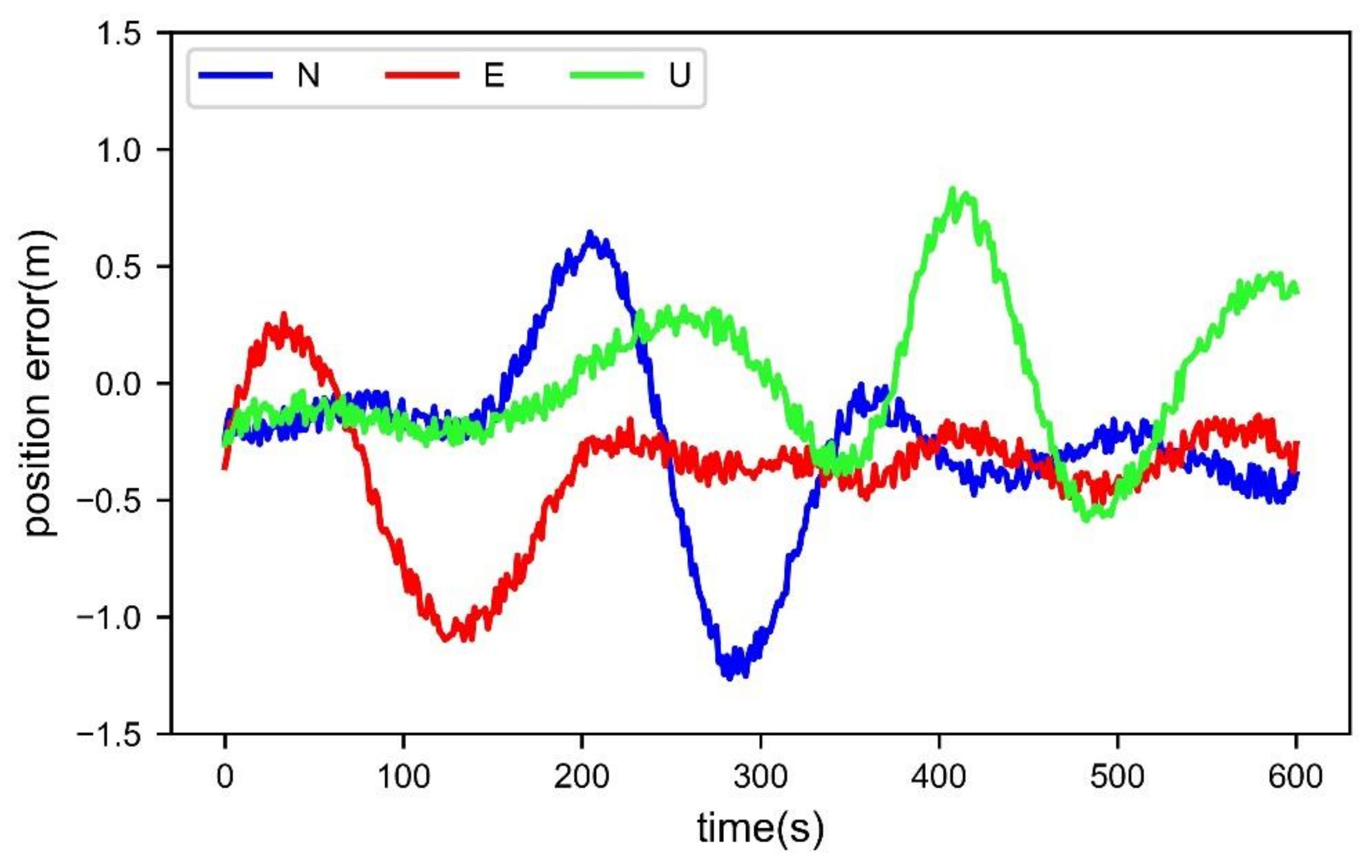
Figure 9 shows the variation in the position error with time for the ORB-SLAM2 [33] without filtering dynamic features. It can be seen that the position error gradually increased with time, which was partly because the feature points changed more drastically during the car driving process. Additionally, the visual odometer naturally had a characteristic of cumulative error drift. It can be seen that the position error of the conventional vision solution can be controlled within 2 m during a 10-min driving time, but there is a tendency for the error to become larger over time. On the other hand, the error in the north (N) direction was predominantly larger than the error in the east (E) direction, mainly because the distance the car travels in the N direction was significantly longer than that in the E direction in that period.

Figure 10 shows the variation in the position error with time for the Dynamic-SLAM algorithm proposed in this study. Compared with the traditional visual localization algorithm, the localization accuracy of Dynamic-SLAM algorithm significantly improved, and the maximum position error was approximately 1.2 m. This is because the Dynamic-SLAM algorithm eliminates the influence of dynamic feature points. Therefore, there was an improvement in the accuracy of both feature matching and depth recovery. Additionally, the loop closing detection module of the Dynamic-SLAM algorithm ensures that the stability of the localization results and reduces the cumulative drift when the acquisition vehicle returns to the same position.

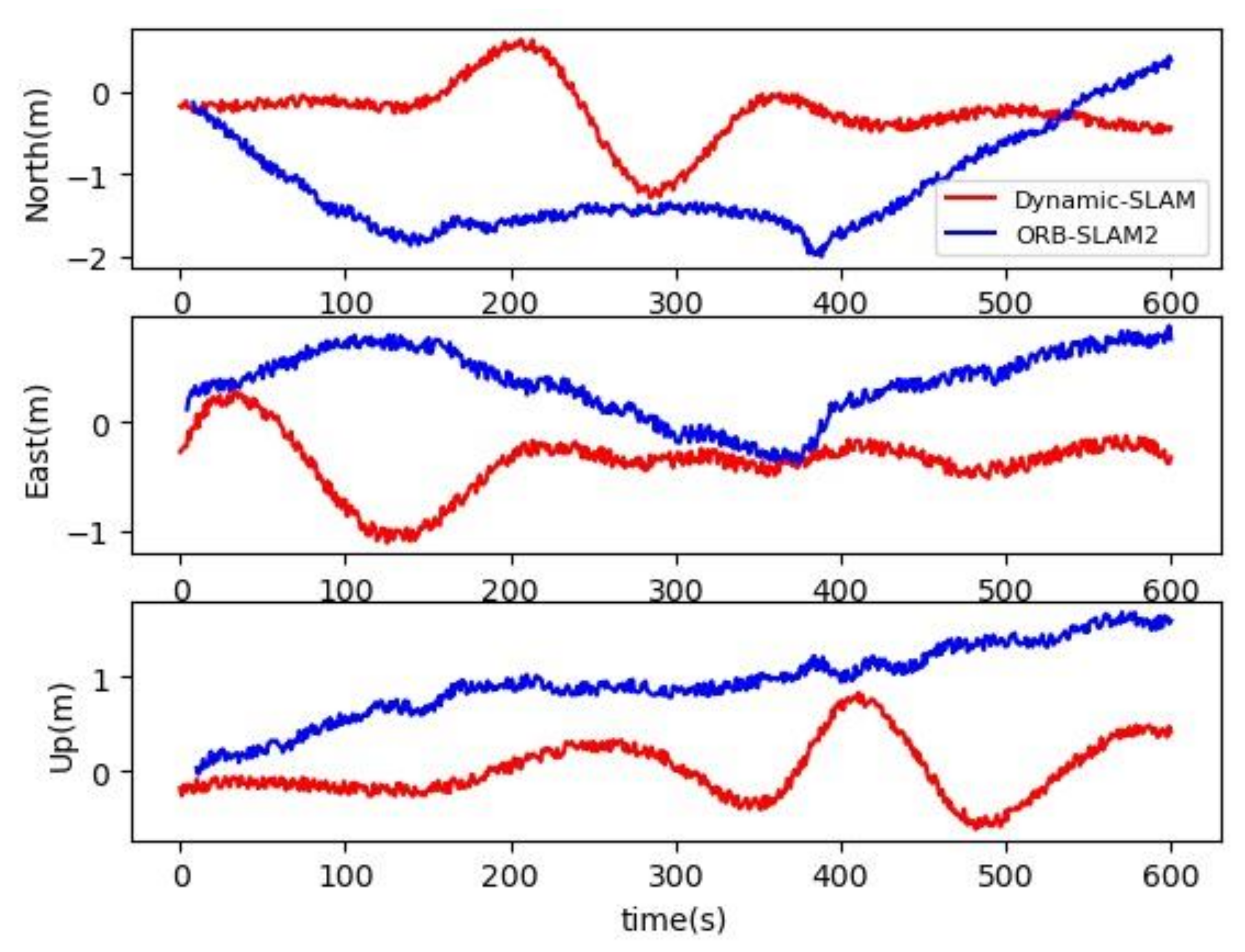
Figure 11 shows the comparison of position error with time between ORB-SLAM2 and Dynamic-SLAM in three directions. Overall, the positions error of dynamic-SLAM is much smaller than ORB-SLAM2. However, the performance of dynamic-SLAM degraded in the east direction from 50 to 150 s. The reason is that a large number of feature points of a parking car were regarded as outliers and filtered out.

The comparison between ORB-SLAM2 and Dynamic-SLAM in terms of the root mean square (RMS) of the position errors is shown in

Table 1. Root mean square (RMS) of the position errors between ORB-SLAM2 and Dynamic-SLAM.

RMS (m)	North	East	Up
ORB-SLAM2	1.326	0.653	1.142
Dynamic-SLAM	0.675	0.715	0.312
Improvement (%)	49.1	−9.49	72.6

, and all the results in Table 1 were calculated by the 10-min experiment data indicated in Figure 6. Obviously, the performance of Dynamic-SLAM was significantly better than ORB-SLAM2. It can be seen that, after adding the semantic segmentation thread, the improvements of RMS of the position differences were approximately 49.1%, −9.49%, 72.6% in the north, east and up directions, respectively. Although the positioning performance was worse in the east direction, the error was still within an acceptable range.

3.2. Positioning Performance of GNSS

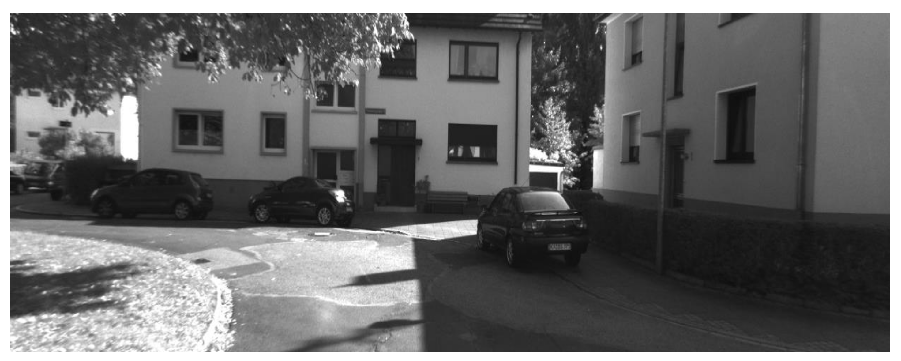
As the acquisition vehicle was driven in an urban environment, the GPS signal was susceptible to occlusion. Figure 12 shows the variation of the position error with time for the dual-frequency RTK in an urban environment. The position error was within 0.03 m from 0 to approximately 150 s, because the GPS signal was better and less obscured during this period. It can be seen that the positioning performance of the RTK was poor from approximately 150 to 450 s, owing to the presence of tall buildings in the environment, as shown in Figure 7. Additionally, the position error in up directions was obviously larger than that in other directions. The reason is that the vertical dilution of precision (VDOP) is usually greater than the horizontal dilution of precision (HDOP) due to the relative position of the satellite and the receiver.

Figure 13 shows the results of a loosely coupled Vision/RTK integration system using the traditional Kalman filter method. Subfigures (a) and (b) represent the whole results and part detailed results, respectively.

By comparing Figure 12 and Figure 13a, the maximum value of position error decreased from approximately 8 to 6 m. This indicates that fusing data from different sensors using a Kalman filter can effectively improve the positioning performance. However, the position accuracy was still poor and could not be accepted by any navigation system. The main problem was that the position error of the RTK was highly deficient when the GPS signals were blocked (from 150 to 220 s and from 280 to 450 s). Furthermore, the position error of the loosely coupled RTK/Vision integration system was within 0.5 m in the horizon direction and within 0.8 m in the vertical direction in open-sky environments, as shown in Figure 13b. Additionally, the visual positioning method inevitably countered the error accumulation over time, as shown in Figure 9. This problem can be solved by integrating it with the GNSS. The reason is that the high-precise position of the RTK can help limit the error of visual positioning algorithm in a relatively small range, which eliminates the cumulative drift.

Although the Kalman filter can effectively improve the positioning performance of each sensor, it requires both the measurement error and the state error to satisfy a Gaussian distribution, resulting in its unsatisfactory performance during GPS signal blocking. Once the GPS signals are blocked, the measurement error will contain a large number of outliers. This does not satisfy the Gaussian distribution, which leads to abnormal filtering and a sharp increase in the position error.

3.3. Positioning Performance of S-AKF

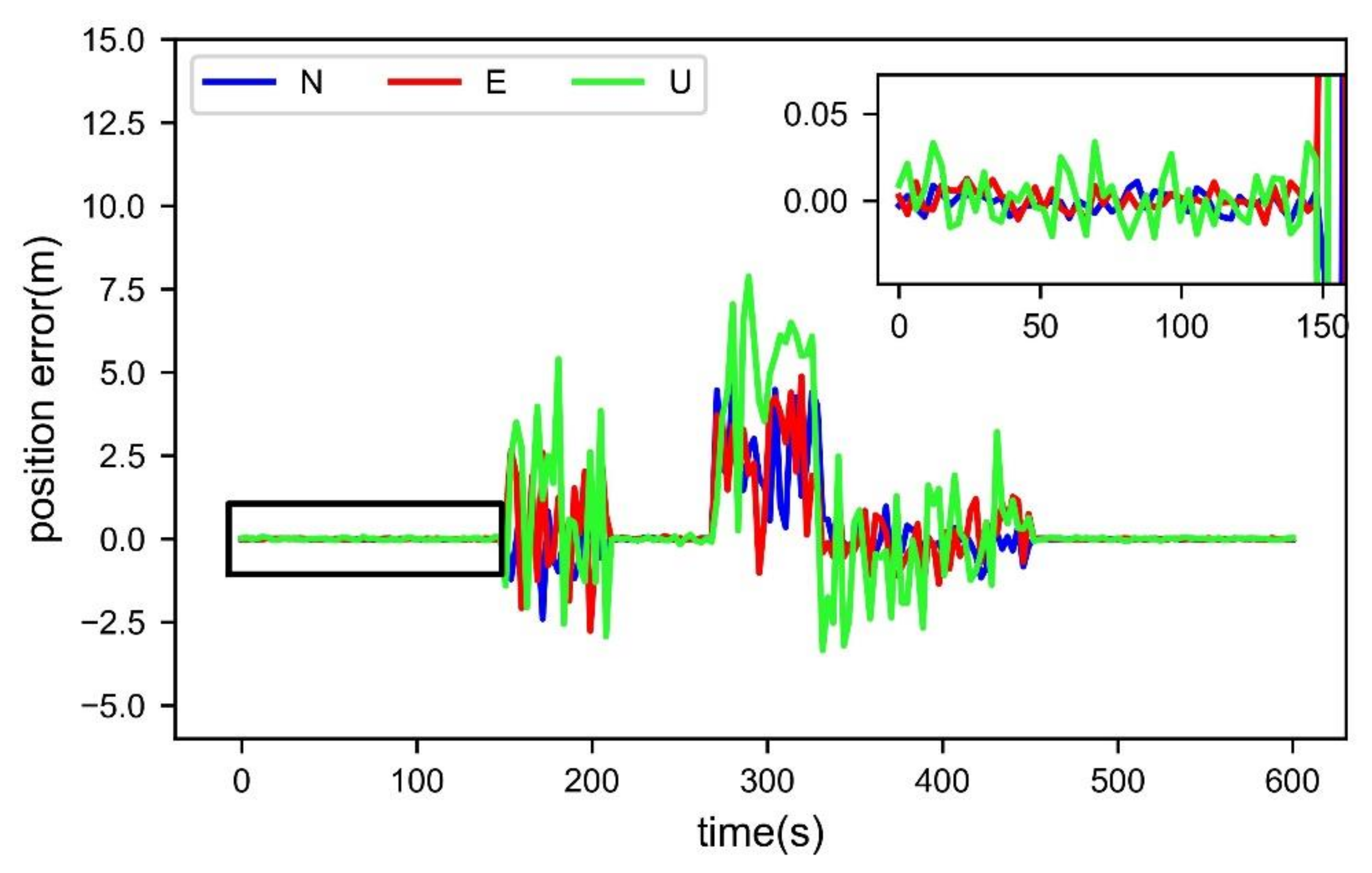
To address the problems with Kalman filtering, we used an S-AKF approach in a loosely coupled GNSS/Vision integration navigation system. Figure 14 shows the variation in the position error of this navigation system over time. As expected, the results of the S-AKF solution were further improved in comparison with those of the traditional Kalman filtering solution. From 150 to 450 s, the semantic segmentation module identified the imminent driving activities in advance in the highly obscured area, dynamically adjusted the measurement noise variance, and updated the Kalman filter gain, which significantly improved the positioning accuracy. During the 10-min drive, the position error of the combined RTK/GNSS navigation system was maintained within 1 m. In the case of GPS signals being blocked, the combined navigation system could achieve continuous high-precision navigation.

Another important conclusion drawn by Figure 13 is that the position errors of the loosely coupled RTK/Vision integration system still accumulated over time when the GPS signals were blocked. From 250 to 450 s, the position error was notably larger than that from 150–200 s. The reason is that GPS signals were blocked longer during the former time. As previously mentioned, the accumulated drifts can be eliminated by the highly precise GNSS; once the GPS signals are blocked, the accumulated drifts were unavoidable. Furthermore, the position error of the RTK/Vision integration system is within 0.05 m during the beginning period from 150 to 200 s, which indicates that the position accuracy could reach centimeter-level if the time of GPS signals being blocked is within approximately 30 s.

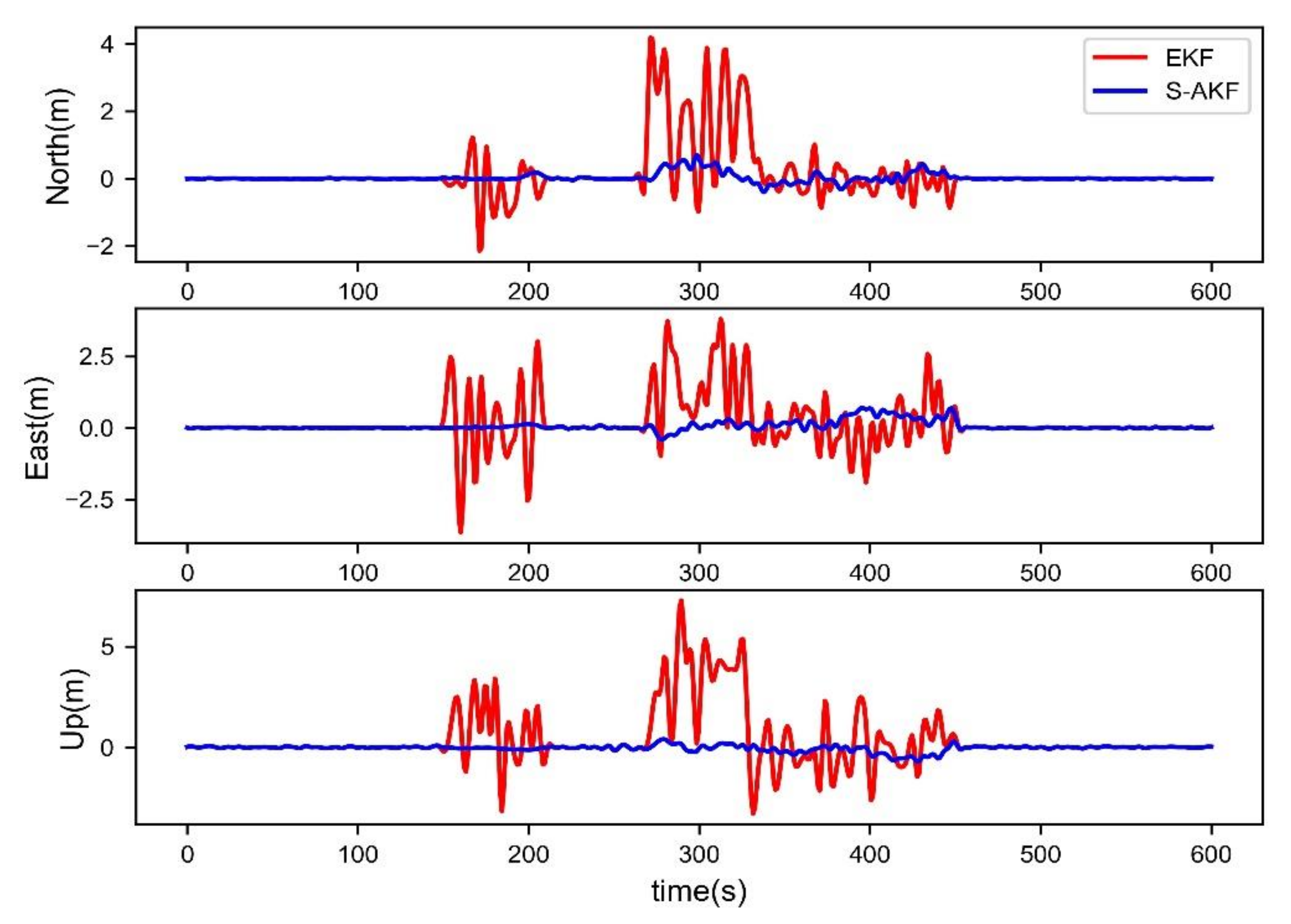
Figure 15 shows the comparison of position error between EKF and S-AKF algorithm. The loosely-coupled RTK/Vision integration using S-AKF performs better than using EKF. The main reason is the S-AKF algorithm can adjust the filter weights adaptively according to the semantic information.

The position difference distribution is an important indicator for evaluating the capability of high-accuracy positioning of an integrated system. To verify the quality of our loosely-coupled RTK/Vision integration solution, we compared it with the tightly coupled RTK/IMU/Vision integration solution proposed in [5]. Figure 16 shows the distribution of the position difference for only the RTK, our loosely coupled RTK/Vision integration solution and tightly coupled RTK/IMU/Vision integration. All position differences were within 0.7 m for the RTK/Vision, whereas approximately 18% and 16% of the position differences were above 0.7 m for RTK and RTK/IMU/Vision, respectively. More importantly, 80% of the position errors were within 0.1 m; the percentage of loosely coupled RTK/Vision integration within 0.1 m increased by approximately 15% compared with that of the RTK alone. Obviously, a stereo camera can significantly improve the high-accuracy positioning capability of GNSS systems. Compared with the RTK/IMU/Vision integration, the percentage within 0.3 m of RTK/Vision is much larger in spite of they have a similar percentage within 0.1 m.

Table 2. Root mean square (RMS) of the position difference of the loosely coupled RTK/Vision integration and the tightly coupled RTK/IMU/Vision integration [5].

RMS (m)	North	East	Up
RTK/IMU/Vision	0.152	0.219	0.065
RTK/Vision	0.143	0.181	0.179
Improvement (%)	5.9	17.3	−175.4

shows the root mean square (RMS) of the position difference of our loosely-coupled RTK/Vision integration solution and the tightly coupled RTK/IMU/Vision integration solution proposed in [5]. Our solution obtained smaller RMS in north and east directions, having a 5.9% and 17.3% improvement, respectively. However, there is a degradation in the up direction for our RTK/Vision integration. The reason is that the addition of IMU can reduce the error in up direction. Nevertheless, the RMS in up direction can be accepted for high-precision positioning. Additionally, our RTK/Vision integration has obvious advantages over the Vision/IMU/Vision integration in terms of the position difference distribution shown in Figure 16.

Table 3. Root mean square (RMS) of the position difference of vision, RTK and the loosely coupled RTK/Vision integration during different periods. Improvements were calculated by the vision and loosely coupled RTK/Vision when the quality of GPS signals was optimal, calculations were performed by the RTK and the loosely coupled RTK/Vision when GPS signal quality is poor.

	GPS-good			GPS-Outages
RMS (m)	North	East	Up	North	East	Up
Vision	0.675	0.715	0.312	0.675	0.715	0.312
RTK	0.011	0.017	0.032	1.578	1.865	2.769
RTK/Vision	0.013	0.016	0.038	0.212	0.274	0.248
	(Compared with Vision)			(Compared with RTK)
Improvement (%)	98.1	97.7	87.8	86.5	85.3	91.1

shows the RMS of the position difference of Vision, RTK and loosely coupled RTK/Vision system during different periods including GPS-good time and GPS-outages time. All the results in Table 3 were calculated by the 10-min experiment data indicated in Figure 6. It is clear that with the aid of vision, the positioning performance of the loosely coupled navigation system had a significantly improvement, especially during the periods when the GPS signals were obscured or even missing. Although, during the period when the GPS signal quality is good, the positioning performance of the combined system was hardly improved compared to RTK alone.

4. Discussion

Sustainable high-precision positioning in complex environments such as cities remains an urgent issue. According to the presented results, the availability of centimeter-level positioning was increased significantly using the loosely coupled GNSS/Vision integration in GNSS-challenged environments.

The position error of the GNSS/Vision combined navigation system was stable within 0.7 m, while the positioning accuracy of the RTK was poor owing to the GPS signals outages, which could not meet the demands for high precision positioning. There were two main reasons for this.

On the one hand, the Dynamic-SLAM algorithm proposed in this study fully utilized the rich information collected by stereo cameras, not only extracting and matching feature points from images, but also analyzing the image semantics and further using the semantic information to segment the dynamic features. According to previous research in the robotics community, the position error of the visual localization algorithm can be significantly reduced when we can segment the dynamic objects in the environment. Our experiments provided evidence for this hypothesis.

On the other hand, semantic information can achieve dynamic adaptive switching between visual positioning algorithms and GNSS positioning algorithms. This is significant for high-accuracy positioning in environments with obscured GPS signals. After the integration of vision, the loosely coupled navigation system maintained high-accuracy positioning in complex urban environments.

5. Conclusions

With the rapid development of unmanned vehicles, there has been a dramatic increase in the demand for high-precision positioning in complex urban environments. Sensor failures can lead to automobile and UAS crashes for high-precision positioning systems. To solve this problem, we proposed a vision-aided GNSS positioning system using semantic information to achieve continuous high-accuracy positioning when occurring GPS failures. Furthermore, the validity of the algorithm was verified using the publicly available KITTI dataset. Based on the experimental results, we obtained the following conclusions.

Through semantic segmentation, the influence of dynamic feature points can be filtered to enhance the robustness and accuracy of the visual localization algorithm, while also providing a priori information for multi-sensors fusion. Through the adaptive filter fusion, our combined navigation system fully exploited the advantages of each sensor. GNSS can help the vision algorithm in eliminating the accumulated position error drift over time. Visual localization can provide more accurate position information when the GPS signal quality is poor or even lost.

According to the experimental results, when the GPS signals were blocked, the loosely coupled RTK/Vision integration system achieved centimeter-level positioning for approximately the first 30 s, and limit the position error to <0.8 m during a total of 200 s.

It should be noted that the positioning performance tended to get worse over the time when GPS signals were blocked. However, considering that the position error of Dynamic-SLAM is within 1 m during the entire 10-min drive, we suggest that the positioning precision can reach centimeter-level during short GPS signal outages (within 30 s), reaching the decimeter-level during long GPS signal outages (within 10 min).

Therefore, it is still not possible to achieve centimeter-level positioning during long GPS outages using our loosely-coupled integration of GNSS and stereo camera. One possible solution is adding IMU to the integration system. The error drift of the vision positioning algorithm can be suppressed under the constraints of IMU.

In future research, we will test our algorithm on more datasets and conduct field vehicular tests. Since we integrated GNSS and stereo camera in a loosely-coupled manner, we can consider using tight coupled to take advantage of the correlations among all the sensor measurements in the future. Additionally, the environment map obtained by visual SLAM can be considered to improve the navigation performance.

References

- Martin, P.G.; Payton, O.D.; Fardoulis, J.S.; Richards, D.A.; Scott, T.B. The use of unmanned aerial systems for the mapping of legacy uranium mines. J. Environ. Radioact. 2015, 143, 135–140. [Google Scholar] [CrossRef] [PubMed] [Green Version]
- Albéri, M.; Baldoncini, M.; Bottardi, C.; Chiarelli, E.; Fiorentini, G.; Raptis, K.G.C.; Realini, E.; Reguzzoni, M.; Rossi, L.; Sampietro, D.; et al. Accuracy of flight altitude measured with low-cost GNSS, radar and barometer sensors: Implications for airborne radiometric surveys. Sensors 2017, 17, 1889. [Google Scholar] [CrossRef] [PubMed] [Green Version]
- Levinson, J.; Askeland, J.; Becker, J.; Dolson, J.; Held, D.; Kammel, S.; Kolter, J.Z.; Langer, D.; Pink, O.; Pratt, V.; et al. Towards fully autonomous driving: Systems and algorithms. In Proceedings of the 2011 IEEE Intelligent Vehicles Symposium (IV), Baden-Baden, Germany, 5–9 June 2011; IEEE: Manhattan, NY, USA, 2011; Volume 108, pp. 163–168. [Google Scholar]
- Li, R.; Liu, J.; Zhang, L.; Hang, Y. LIDAR/MEMS IMU integrated navigation (SLAM) method for a small UAV in indoor environments. In Proceedings of the 2014 DGON Inertial Sensors and Systems (ISS), Karlsruhe, Germany, 16–17 September 2014. [Google Scholar] [CrossRef]
- Li, T.; Zhang, H.; Gao, Z.; Niu, X.; El-Sheimy, N. Tight fusion of a monocular camera, mems-imu, and single-frequency multi-gnss rtk for precise navigation in gnss-challenged environments. Remote Sens. 2019, 11, 610. [Google Scholar] [CrossRef] [Green Version]
- Hsu, L.T. Analysis and modeling GPS NLOS effect in highly urbanized area. GPS Solut. 2018, 22, 1–12. [Google Scholar] [CrossRef] [Green Version]
- Niu, X.; Zhang, Q.; Gong, L.; Liu, C.; Zhang, H.; Shi, C.; Wang, J.; Coleman, M. Development and evaluation of gnss/ins data processing software for position and orientation systems. Surv. Rev. 2015, 47, 87–98. [Google Scholar] [CrossRef]
- Gao, Z.; Ge, M.; Shen, W.; Zhang, H.; Niu, X. Ionospheric and receiver DCB-constrained multi-GNSS single-frequency PPP integrated with MEMS inertial measurements. J. Geod. 2017, 91, 1351–1366. [Google Scholar] [CrossRef]
- Chiang, K.W.; Duong, T.T.; Liao, J.K. The performance analysis of a real-time integrated INS/GPS vehicle navigation system with abnormal GPS measurement elimination. Sensors 2013, 13, 10599–10622. [Google Scholar] [CrossRef] [PubMed] [Green Version]
- Zhang, G.; Hsu, L.T. Intelligent GNSS/INS integrated navigation system for a commercial UAV flight control system. Aerosp. Sci. Technol. 2018, 80, 368–380. [Google Scholar] [CrossRef]
- Meng, Y.; Gao, S.; Zhong, Y.; Hu, G.; Subic, A. Covariance matching based adaptive unscented Kalman filter for direct filtering in INS/GNSS integration. Acta Astronaut. 2016, 120, 171–181. [Google Scholar] [CrossRef]
- Falco, G.; Gutiérrez, M.C.C.; Serna, E.P.; Zacchello, F.; Bories, S. Low-cost real-time tightly-coupled GNSS/INS navigation system based on carrier-phase double differences for UAV applications. In Proceedings of the 27th International Technical Meeting of the Satellite Division of the Institute of Navigation (ION GNSS+ 2014), Tampa, FL, USA, 8–12 September 2014; Volume 1, pp. 841–857. [Google Scholar]
- Eling, C.; Klingbeil, L.; Kuhlmann, H. Real-time single-frequency GPS/MEMS-IMU attitude determination of lightweight UAVs. Sensors 2015, 15, 26212–26235. [Google Scholar] [CrossRef] [PubMed] [Green Version]
- Li, T.; Zhang, H.; Gao, Z.; Chen, Q.; Niu, X. High-accuracy positioning in urban environments using single-frequency multi-GNSS RTK/MEMSIMU integration. Remote Sens. 2018, 10, 205. [Google Scholar] [CrossRef] [Green Version]
- Davison, A.J.; Reid, I.D.; Molton, N.D.; Stasse, O. MonoSLAM: Real-time single camera SLAM. IEEE Trans. Pattern Anal. Mach. Intell. 2007, 29, 1052–1067. [Google Scholar] [CrossRef] [PubMed] [Green Version]
- Chiuso, A.; Favaro, P.; Jin, H.; Soatto, S. Structure from motion causally integrated over time. IEEE Trans. Pattern Anal. Mach. Intell. 2002, 24, 523–535. [Google Scholar] [CrossRef]
- Mur-Artal, R.; Montiel, J.M.M.; Tardos, J.D. ORB-SLAM: A versatile and accurate monocular SLAM system. IEEE Trans. Robot. 2015, 31, 1147–1163. [Google Scholar] [CrossRef] [Green Version]
- Mouragnon, E.; Lhuillier, M.; Dhome, M.; Dekeyser, F.; Sayd, P. Real time localization and 3D reconstruction. Proc. IEEE Comput. Soc. Conf. Comput. Vis. Pattern Recognit. 2006, 1, 363–370. [Google Scholar] [CrossRef] [Green Version]
- Klein, G.; Murray, D. Parallel tracking and mapping for small AR workspaces. In Proceedings of the 2007 6th IEEE and ACM International Symposium on Mixed and Augmented Reality, Nara, Japan, 13–16 November 2007; pp. 225–234. [Google Scholar] [CrossRef]
- Mur-Artal, R.; Tardós, J.D. Fast relocalisation and loop closing in keyframe-based SLAM. In Proceedings of the 2014 IEEE International Conference on Robotics and Automation (ICRA), Hong Kong, China, 31 May–7 June 2014; pp. 846–853. [Google Scholar] [CrossRef] [Green Version]
- Lee, W.; Eckenhoff, K.; Geneva, P.; Huang, G. Intermittent GPS-aided VIO: Online initialization and calibration. In Proceedings of the 2020 IEEE International Conference on Robotics and Automation (ICRA), Paris, France, 31 May–31 August 2020; pp. 5724–5731. [Google Scholar] [CrossRef]
- Cioffi, G.; Scaramuzza, D. Tightly-coupled fusion of global positional measurements in optimization-based visual-inertial odometry. In Proceedings of the 2020 IEEE/RSJ International Conference on Intelligent Robots and Systems (IROS), Las Vegas, NV, USA, 25–29 October 2020; pp. 5089–5095. [Google Scholar] [CrossRef]
- Qin, T.; Cao, S.; Pan, J.; Shen, S. A general optimization-based framework for global. arXiv 2019, arXiv:1901.03642. [Google Scholar]
- Mascaro, R.; Teixeira, L.; Hinzmann, T.; Siegwart, R.; Chli, M. GOMSF: Graph-optimization based multi-sensor fusion for robust UAV pose estimation. In Proceedings of the 2018 IEEE International Conference on Robotics and Automation (ICRA), Brisbane, QLD, Australia, 21–25 May 2018; Volume 644128, pp. 1421–1428. [Google Scholar] [CrossRef] [Green Version]
- Weiss, S.; Achtelik, M.W.; Chli, M.; Siegwart, R. Versatile distributed pose estimation and sensor self-calibration for an autonomous MAV. In Proceedings of the 2012 IEEE International Conference on Robotics and Automation, Saint Paul, MN, USA, 14–18 May 2012; IEEE: Manhattan, NY, USA, 2012; pp. 31–38. [Google Scholar]
- Lynen, S.; Achtelik, M.W.; Weiss, S.; Chli, M.; Siegwart, R. A robust and modular multi-sensor fusion approach applied to MAV navigation. In Proceedings of the 2013 IEEE/RSJ International Conference on Intelligent Robots and Systems, Tokyo, Japan, 3–7 November 2013; pp. 3923–3929. [Google Scholar] [CrossRef] [Green Version]
- Bloesch, M.; Omari, S.; Hutter, M.; Siegwart, R. Robust visual inertial odometry using a direct EKF-based approach. In Proceedings of the IEEE International Conference on Intelligent Robots and Systems, Hamburg, Germany, 28 September–2 October 2015; IEEE: Manhattan, NY, USA, 2015; Volume 2015, pp. 298–304. [Google Scholar]
- Kim, J.; Sukkarieh, S. SLAM aided GPS/INS navigation in GPS denied and unknown environments. In Proceedings of the GNSS 2004 The 2004 International Symposium on GNSS/GPS, Sydney, Australia, 6–8 December 2004. [Google Scholar]
- Chu, T.; Guo, N.; Backén, S.; Akos, D. Monocular camera/IMU/GNSS integration for ground vehicle navigation in challenging GNSS environments. Sensors 2012, 12, 3162–3185. [Google Scholar] [CrossRef] [PubMed]
- Li, X.; Wang, X.; Liao, J.; Li, X.; Li, S.; Lyu, H. Semi-tightly coupled integration of multi-GNSS PPP and S-VINS for precise positioning in GNSS-challenged environments. Satell. Navig. 2021, 2, 1–14. [Google Scholar] [CrossRef]
- Shepard, D.P.; Humphreys, T.E. High-precision globally-referenced position and attitude via a fusion of visual SLAM, carrier-phase-based GPS, and inertial measurements. In Proceedings of the 2014 IEEE/ION Position, Location and Navigation Symposium—PLANS 2014, Monterey, CA, USA, 5–8 May 2014; pp. 1309–1328. [Google Scholar] [CrossRef] [Green Version]
- Levinson, J.; Montemerlo, M.; Thrun, S. Map-based precision vehicle localization in urban environments. Robot. Sci. Syst. 2008, 3, 121–128. [Google Scholar] [CrossRef]
- Mur-Artal, R.; Tardos, J.D. ORB-SLAM2: An open-source SLAM system for monocular, stereo, and RGB-D cameras. IEEE Trans. Robot. 2017, 33, 1255–1262. [Google Scholar] [CrossRef] [Green Version]
Figure 1.
The framework of dynamic simultaneous localization and mapping (Dynamic-SLAM). The local mapping thread processes new keyframes and performs local bundle adjustment to achieve an optimal reconstruction in the surroundings of the camera pose. The loop closing thread searches for loops and performs a graph optimization if a loop is detected. The tracking thread extracts and matches the features to localizing the camera. VO module processes frames to obtain pose estimation.
Figure 2.
Pipeline of our loosely-coupled Global Navigation Satellite System (GNSS)/Vision integration system.
Figure 3.
Semantic image. The prioritydynamic objects, such as pedestrians and vehicles, can be identified and segmented out.
Figure 4.
Algorithm structure of the loosely coupled integration of stereo camera and GNSS receiver. GNSS: global navigation satellite system; RTK: real-time kinematics; : The state vector consists of the position errors and the velocity errors in north, east and up directions. k: the occlusion factor calculated by semantic segmentation.
Figure 5.
Recording Platform. The Recording Platform is equipped with two stereo camera rigs (one for grayscales and one for color) and a GPS/IMU localization unit with RTK correction signals.
Figure 6.
Recording Zone. Colors encode the GPS signal quality: Red tracks have been recorded with highest precision using RTK corrections in open-sky environment, blue denotes the intermittent access to GPS signals in GPS-challenge environment, black denotes no access to GPS signals. The closed tracks indicated by the red arrow are our experiment data.
Figure 7.
Typical obscured scene. The buildings in the figure and also the shade of trees can block the GPS signal propagation and affect the performance of RTK.
Figure 8.
Feature image before and after excluding features on dynamic objects. The above image is the reasult extracting features using ORB-SLAM2. The below image is the result extracting features using Dynamic-SLAM. In the below image, dynamic objects like pedestrian, bicycle and car are segmented out, on which there are no feature points.
Figure 9.
Position error of ORB-SLAM2 in the north (N), east (E), and up (U) directions.
Figure 10.
Position error of Dynamic-SLAM in the north (N), east (E), and up (U) directions.
Figure 11.
Comparison of position error between Dynamic-SLAM and ORB-SLAM2 in the north (N), east (E), and up (U) directions.
Figure 12.
Position error of the RTK in the north (N), east (E), and up (U) directions. The zoom graph from 0 to 150 s is in the upper right corner.
Figure 13.
Position error of loosely coupled RTK/Vision integration using traditional Kalman filter. (a) Position error during the whole 10 minutes, including in open-sky environments and GNSS-challenged environments, the rectangular box represents the enlarged part shown in (b); (b) position error during the starting 80 seconds, only in open-sky environments.
Figure 14.
Position error of vision aided GNSS using semantic-adaptive Kalman filter in the north (N), east (E), and up (U) directions.
Figure 15.
Position error of loosely-coupled RTK/Vision integration using EKF and S-AKF in the north (N), east (E), and up (U) directions.
Figure 16.
Distribution of the position difference of RTK, RTK/Vision integration and RTK/IMU/Vision integration [5].