
NDSRGAN: A Novel Dense Generative Adversarial Network for Real Aerial Imagery Super-Resolution Reconstruction


1
School of Computer Science, China University of Geosciences, Wuhan 430074, China
2
School of Geography and Information Engineering, China University of Geosciences, Wuhan 430074, China
3
National Engineering Research Center of Geographic Information System, Wuhan 430074, China
4
Key Laboratory of Urban Land Resources Monitoring and Simulation, Ministry of Natural Resources, Shenzhen 518034, China
5
Wuhan Zondy Advanced Technology Institute Co., Ltd., Wuhan 430074, China
*
Author to whom correspondence should be addressed.
Remote Sens. 2022, 14(7), 1574; https://doi.org/10.3390/rs14071574
Submission received: 7 February 2022
/
Revised: 14 March 2022
/
Accepted: 23 March 2022
/
Published: 24 March 2022
(This article belongs to the Topic High-Resolution Earth Observation Systems, Technologies, and Applications)
Abstract
:In recent years, more and more researchers have used deep learning methods for super-resolution reconstruction and have made good progress. However, most of the existing super-resolution reconstruction models generate low-resolution images for training by downsampling high-resolution images through bicubic interpolation, and the models trained from these data have poor reconstruction results on real-world low-resolution images. In the field of unmanned aerial vehicle (UAV) aerial photography, the use of existing super-resolution reconstruction models in reconstructing real-world low-resolution aerial images captured by UAVs is prone to producing some artifacts, texture detail distortion and other problems, due to compression and fusion processing of the aerial images, thereby resulting in serious loss of texture detail in the obtained low-resolution aerial images. To address this problem, this paper proposes a novel dense generative adversarial network for real aerial imagery super-resolution reconstruction (NDSRGAN), and we produce image datasets with paired high- and low-resolution real aerial remote sensing images. In the generative network, we use a multilevel dense network to connect the dense connections in a residual dense block. In the discriminative network, we use a matrix mean discriminator that can discriminate the generated images locally, no longer discriminating the whole input image using a single value but instead in chunks of regions. We also use loss instead of the loss used in most existing super-resolution models, to accelerate the model convergence and reach the global optimum faster. Compared with traditional models, our model can better utilise the feature information in the original image and discriminate the image in patches. A series of experiments is conducted with real aerial imagery datasets, and the results show that our model achieves good performance on quantitative metrics and visual perception.
1. Introduction
Unmanned aerial vehicle (UAV) aerial remote sensing images can provide information about the Earth’s surface quickly, but medium- and low-resolution UAV aerial imagery has limitations regarding extraction of high-precision features, map updates and target detection. The development of high-resolution UAV aerial imagery makes the in-depth application of aerial imagery possible, thus providing favourable conditions for GIS data updates [1] and GIS applications [2]. It is also important for map updates [3], semantic segmentation [4] and target detection [5]. Computer vision technology has been widely applied in many fields such as multi-target recognition [6] and seismic performance evaluation [7].
In the field of aerial photography, obtaining high-resolution aerial images is difficult due to the influence of imaging technology and photographic equipment [8], which often requires UAVs to perform ultra-low-altitude aerial photography, a process that is both labour-intensive and costly. As a result, techniques to achieve super-resolution (SR) reconstruction of images from an algorithmic point of view have become an important research topic in various fields such as image processing and computer vision [9]. However, most of the existing super-resolution reconstruction models generate low-resolution images for training by downsampling high-resolution images through bicubic interpolation, and the models trained from these data have poor reconstruction results on real-world low-resolution images.
To solve this problem, we propose NDSRGAN. Unlike previous GAN-based image SR reconstruction models, this model has a dense connection in the residual dense block (DCRDB) in the generative network, which consists of multilevel dense connections (MDC) and residual connections [10]. Multiple DCRDBs are then connected by a multilevel dense network to form a generative network, which is optimised to enable the generative network to fully utilise the feature information of real aerial images. The discriminator is specially designed using a matrix mean discriminator (MMD) network, which discards the full connection of the last layer of the traditional discriminator and outputs a discriminator matrix instead, where each value of the matrix represents a piece of the receptive field in the image. In the objective function, we use loss instead of the loss used in most image SR reconstruction models. This can better accelerate the convergence of the model to reach the global optimum [11].
Most existing image SR reconstruction models use LR images generated by bicubic interpolation using HR images, which are very different from the low-resolution images obtained by actual photography. To ensure that our model met the requirements of practical applications, we did not use LR images generated by bicubic interpolation paired with HR images for training. Instead, we created the dataset by using LR images and HR images of the real shots to perform training. In the reconstruction of the real aerial imagery dataset and benchmark dataset, our model achieved the best SR reconstruction results, compared with representative image SR reconstruction models.
Specifically, the main contributions of this work are as follows:
- We produce a new image dataset with paired high- and low-resolution real aerial remote sensing images, which are both obtained by actual photography.
- We propose a novel dense generative adversarial network for real aerial imagery super-resolution reconstruction (NDSRGAN). In the generative network, we use a multilevel dense network to connect the dense connections in a residual dense block. In the discriminative network, we use a matrix mean discriminator that can discriminate the generated images locally. We also use loss to accelerate the model convergence and reach the global optimum faster.
The rest of the paper is organised as follows. Related studies on super-resolution are introduced in Section 2. In Section 3, we detail our NDSRGAN. The datasets and experimental results are given in Section 4, and we discuss our method on an open-source dataset in Section 5. Finally, we conclude our work and discuss future research directions in Section 6.
2. Related Work
The main SR methods are divided into three categories, which are discussed in the following subsections.
2.1. Interpolation-Based Methods
Interpolation-based methods calculate the value of a point according to a certain formula by using the values of several known points around the point and the relationship between the surrounding points and the location of this point. Interpolation-based methods are simple, efficient and easy to understand, but they are also prone to blurring and jaggedness when recovering images, and they cannot recover image details because no new information is generated during the interpolation process. Common interpolation-based methods include nearest neighbour [12], bilinear [13] and bicubic [14] methods.
2.2. Reconstruction-Based Methods
Reconstruction-based methods establish an observation model for the process of converting high-resolution (HR) images into low-resolution (LR) images, and then achieve SR reconstruction by solving the inverse problem of the observation model. Typical reconstruction-based methods are nonuniform interpolation [15], iterative inverse projection [16], maximum posterior probability [17] and convex set projection [18] methods.
2.3. Learning-Based Methods
A learning-based image SR algorithm learns the mapping relationship between LR and HR images by training the image dataset to predict the missing details of feature information in LR images to reconstruct high-quality images. Learning-based SR methods are the mainstream research direction at present, and they achieve the best results. Commonly used learning-based SR methods include the neighbour embedding method [19], sparse representation [20] and deep learning [21].
In recent years, with the rapid development of artificial intelligence technology [22], the use of deep learning methods to achieve SR reconstruction has become mainstream, and many deep-neural-network-based models have made good progress in the field of SR reconstruction. The methods using deep learning for single-image SR reconstruction [23] can be further divided into two categories: convolutional neural network (CNN)-based SR reconstruction and generative adversarial network (GAN)-based SR reconstruction.
2.3.1. CNN-Based SR Reconstruction Methods
A simple SRCNN was proposed by Dong et al. [24], which used a simple three-layer CNN [25] to achieve SR reconstruction and obtained better reconstruction results than traditional methods. However, due to the large size of the convolutional kernel and the shallow depth of the network, the reconstructed image was too smooth, and the reconstruction details were lost.
To overcome this shortcoming, Dong et al., proposed a fast SR reconstruction CNN (FSRCNN) [26], which uses smaller convolutional kernels than SRCNN to complete feature extraction and nonlinear mapping of images, and abandons the initial interpolation of low-resolution images for enlargement, instead directly inputting low-resolution images and finally performing deconvolution [27] to amplify the image. After this series of optimisations, FSRCNN obtained a higher evaluation score and better reconstruction effect than SRCNN. However, the reconstruction details still require improvement because the network structure is too simple.
Following the wide application of residual networks (ResNet) [28] in the field of target detection and target recognition, Lim et al. applied ResNet to the field of image SR reconstruction and proposed an enhanced SR reconstruction residual network (EDSR) [29]. In this network, the authors removed the batch normalisation (BN) layer from the ResNet [30] and increased the number of residual layers from 16 to 32. The BN layer consumes the same amount of memory as its preceding convolutional layers. Thus, after this operation step is removed, EDSR can stack more network layers, so that more features are extracted per layer with the same computational resources, resulting in a better performance.
These CNN-based SR network models have made good progress in continuous optimisation and improvement. However, a common loss function for CNN-based SR network models is the mean squared error (MSE), which causes the generated images to have a high signal-to-noise ratio but lack high-frequency detail and have an over-smoothed texture.
2.3.2. GAN-Based SR Reconstruction Methods
Compared with traditional CNNs, the biggest difference and success of GANs is the discriminator, which can be trained to discriminate the input generated images. In the field of aerial photography, the image complexity in aerial images is greater than that in natural images [31]. Conventional discriminators are prone to local discriminative errors in discriminating images. They cannot make correct discriminations based on the correlation of surrounding features, thus seriously affecting the quality of generated high-resolution images.
The main structure of a GAN consists of a generator and a discriminator. The generator generates fake images that deceive the discriminator, and the discriminator discriminates whether the input image is from a real image or a fake image generated by the generator, to achieve Nash equilibrium [32] by alternately training the generator and the discriminator, finally determining the network model parameters [33].
Ledig proposed a single-image SR reconstruction method using GANs (SRGAN) [34], which was the first application of GANs in image SR reconstruction, to solve the shortcomings of MSE in CNN-based SR reconstruction models [35]. SRGAN uses perceptual loss as an optimisation objective. Perceptual loss was proposed by Johnson et al., inspired by the studies in [36,37], and consists of adversarial loss [33] and content loss. Adversarial loss maps the image to a high-dimensional feature space and uses a discriminative network to discriminate the reconstructed image from the original image, and content loss is based on receptive similarity rather than pixel similarity [38].
An activated 19-layer VGG network [39] is used to obtain the feature maps of the generated image and the original high-resolution image, and then to improve the quality of the generated image by minimising the error between the generated image and the feature maps of the original high-resolution image. However, because the generative network of SRGAN partly uses ResNet, the generated image is usually not sufficiently natural and contains some noise.
To address the shortcomings of SRGAN, Wang et al., proposed an enhanced SRGAN (ESRGAN) [40]. This uses a multilevel network structure unit RRDB instead of ResNet in the generative network of the SRGAN and removes the BN layer. Inspired by a relativistic GAN, it allows the discriminator to predict the probability that the generated image is more false, relative to the high-resolution image, rather than just the probability that the generated image is false [41]. It also uses feature maps with stronger supervisory information before activation, to constrain the perceptual loss function. After a series of optimisations, the ESRGAN model achieved better visual quality in its reconstructed images but did not reconstruct more desirable results for the edge contours of some features. Therefore, Ma et al., proposed a gradient-guided SR reconstruction network model (SPSR) [42], which adds a gradient branch and gradient loss to the ESRGAN network and can recover the contour details of the original image to a great extent.
However, the overall visual effect of the image is still different from that of the original image. Although the above research on GAN SR models has achieved great improvements in the SR effect, the mainstream models usually use some more basic residual networks and L1 loss, resulting in the inability to fully learn the features of the real aerial images, while most models ignore the optimisation of the discriminator.
3. Method
This section focuses on the design of the generative network, discriminative network and loss function of NDSRGAN.
3.1. Generative Network
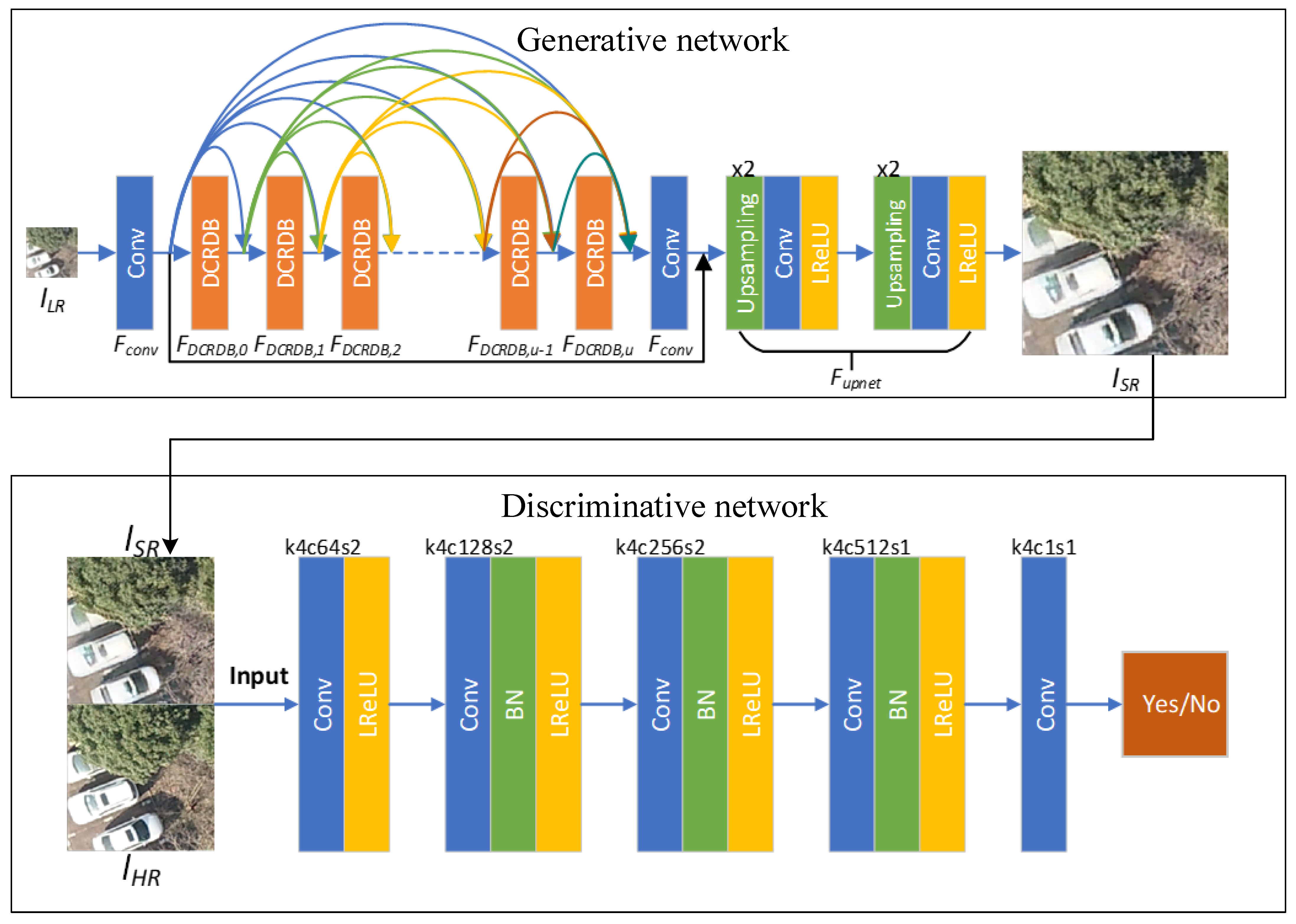
The generative network architecture is shown in Figure 1. Firstly, we use one convolutional layer to extract the original features in the LR image to obtain the original feature maps . is further input into multiple DCRDBs connected by a dense network. Then, the input and output of the u-th DCRDB can be represented as follows:
In Equation (1), represents the original feature maps of the LR image after convolution and represents the residual scaling factor [43]. In Equation (2), represents the input of the u-th DCRDB, represents the output of the u-th DCRDB and represents the composite network formed by the u-th DCRDB through dense connections.
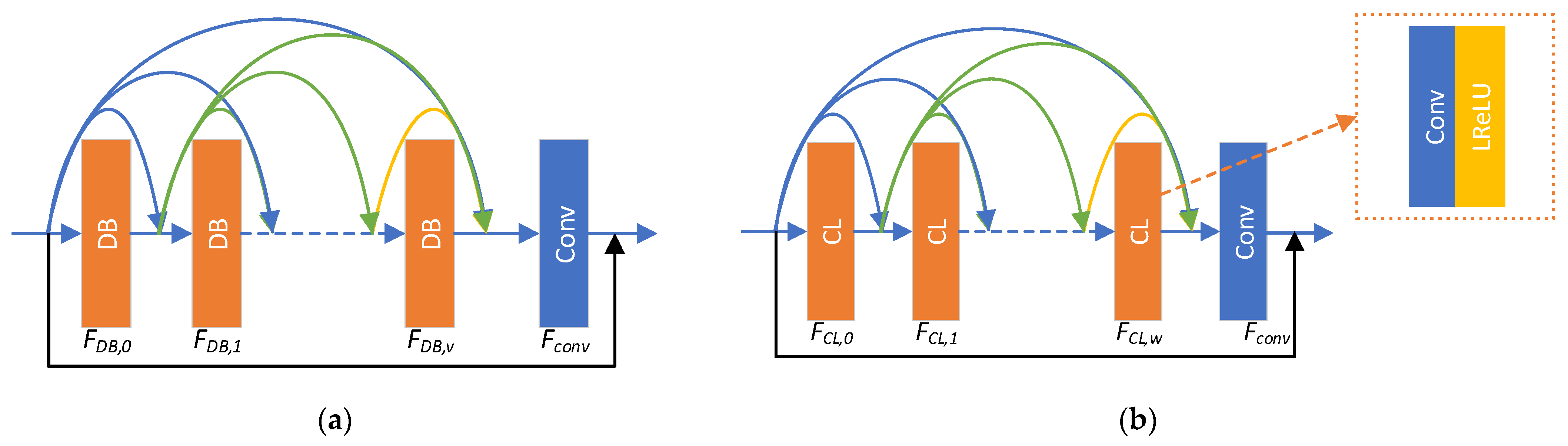
The specific network structure of the DCRDB is shown in Figure 2a. Each DCRDB consists of dense blocks (DB) and a convolutional layer, connected using a dense network. These dense connections can ensure that the output feature maps of each dense block module can be reused in multiple levels, which can maximise the use of feature information on LR images. The v-th DCRDB internal calculation formula can be described as follows:
In Equation (4), is the input of the v-th layer of the DB in the u-th DCRDB, is the output of the v-th layer of the DB in the u-th DCRDB and represents the v-th layer of the DB in the u-th DCRDB. After this, we sum the outputs of the DBs through the dense connection and input them into the convolutional layer, which is calculated as follows:
In Equation (5), represents the last convolutional operation in the DCRDB and represents the output of the convolutional layer, immediately after which we access a residual connection, calculated as follows:
In Equation (6), represents the input after the u-th DCRDB and represents the output after the u-th DCRDB.
The DB structure is shown in Figure 2b. Each DB is composed of a series of CL modules and a convolutional layer, with dense connection. The CL module consists of a convolutional layer and a leaky ReLU (LReLU) layer [44,45]. The internal computational formula of the v-th DB in the u-th DCRDB can be described as
In Equation (8), is the input of the w-th CL module in the v-th dense block in the u-th DCRDB, is the output of the w-th CL module in the v-th dense block in the u-th DCRDB, represents the w-th CL composite network in the v-th DB of the u-th CRDB and represents the concatenate operation that sums the channels of the input feature maps. Suppose we use CL modules, then:
In Equation (9), is the output of and is the last layer of the convolution operation of the DB. Following this, we access a residual connection
In Equation (10), is the input of the v-th DB in the u-th DCRDB and is the output of the v-th dense block in the u-th DCRDB.
After introducing the basic components of the DCRDB, we now introduce the generative network. Suppose we use DCRDBs. The output is connected with the output of each previous layer of DCRDBs and fed into the next convolutional layer:
In Equation (11), represents the final layer of the convolution operation of the generative network and represents the output of . Then, we access a residual connection
In Equation (12), represents the output of connected to the residuals. Finally, is fed to the upsampling network, set up as follows:
In Equation (13), represents our upsampling network, represents the input of the upsampling network and represents the output of the upsampling network, which is also the input of the final discriminator. The upsampling network of ESRGAN [40] is exploited in our network. It includes two magnification steps. Each step uses a nearest neighbour algorithm to magnify the image and connect a convolutional layer and an LReLU [44,45] layer.
3.2. Discriminative Network
The role of the discriminator is to discriminate the feature map distribution difference between and , and to discriminate whether is real or fake. The output of the basic discriminator of a GAN is often a classification after a series of convolutions and a full concatenation score to indicate whether the overall category of the image is real or fake. The receptive field for classification is the whole image, which is why the network is insensitive to the local information of the image and cannot achieve a higher-fidelity image reconstruction in the case of rich feature details. Therefore, local feature extraction and discrimination of the image are needed to generate an SR reconstructed image that is closer to the real aerial image.
Inspired by [46], we used the idea of a matrix mean discriminator capable of local discrimination on the generated images, to construct our discriminative network. The network structure of the discriminative network is shown in Figure 1, set up as a fully convolutional network [47]. The first layer consists of a convolutional layer and an LReLU [44,45]. The second, third and fourth layers consist of a convolution layer, a BN layer and an LReLU [44,45]. The fifth layer consists of one convolutional layer. The size of the output matrix in each layer is shown in Table 1.
The discriminative network finally yields an discriminative matrix. Each element in the matrix represents a receptive field in the original image and carries out a real or fake discrimination for each value in the matrix to complete the local discrimination of the input image. The experimental results shown in Section 4 demonstrate that the image quality is significantly improved by our discriminator-optimised model.
3.3. Loss Function Design
Here, we introduce the design of the loss function of the generative network, which consists of three main parts: pixel loss, perceptual loss [38] and adversarial loss [33]. Pixel loss is calculated as follows:
In which
Is a more powerful objective function. In fact, in the interval of , loss actually solves the problem of a too-large gradient and unstable training caused by a too-large difference between and at the early stage of training. In the interval, which is actually loss, the derivative of the loss is relatively small when the difference between and is small in the late training period, thereby making the loss convergence more stable and aiding convergence to the global optimum [11]. The perceptual loss is calculated as follows:
We use the loss to design our perceptual loss. In Equation (16), represents a 19-layer VGG network [39], and we use this network before activation to extract the feature maps from the generated and real images. The goal of the perceptual loss function is to minimise the error between the feature maps. The addition of this loss function allows our model to generate images with a more realistic texture. We can now introduce the adversarial loss for the generator, which is calculated as follows:
In Equation (17), represents the difference between the matrix of the real image output through the discriminator and the element mean of the output matrix of after the discriminator . Then, the resultant matrix is mapped to a probability matrix between 0 and 1 by the sigmoid function, and the matrix has an optimisation target of 0 for each element. Each element represents an optimisation target of 0 for each receptive field. Here, is the sigmoid function and represents the difference between the matrix of output through the discriminator and the element mean of the output matrix of after the discriminator . Afterwards, the resultant matrix is mapped to a probability matrix between 0 and 1 by the sigmoid function, and the optimisation target of each element in the matrix is 1. Each element also represents an optimisation target of 1 for each receptive field. The optimisation target of the receptive field is 1. The final objective function of the generator can be defined as
In Equation (18), and represent the weight coefficients of the pixel loss and the generator adversarial loss.
Next, we introduce the discriminator loss function construction. The discriminator adversarial loss calculation formula can be expressed as
The design of the discriminator adversarial loss differs from that of the generator in which each element of the output matrix has an optimisation objective of 1, in that each element of the output matrix has an optimisation objective of 0. The similarity lies in the fact that each element of the matrix represents each receptive field. The loss function of the discriminator can be expressed as
In Equation (20), represents the weight coefficient of . We optimise and by alternate training to update the parameters of our generative and discriminative networks and obtain our SR reconstruction model.
4. Experiments and Results
In this section, we introduce the production of the SR reconstruction dataset based on real HR and LR aerial imagery (RHLAI), the details of training parameters, the analysis of changes in the reconstructed image quality metrics during NDSRGAN training and the analysis of the reconstruction results of the RHLAI dataset.
4.1. RHLAI Dataset
Most SR reconstruction methods use LR images obtained by bicubic interpolation of HR images. A difference exists between the LR images obtained in this way and the actual LR images. As a result, the trained SR models often do not have the SR reconstruction capability of the real LR images. To solve this problem, in this study we discarded the bicubic interpolation method of generating LR images from HR images used in most previous studies to construct paired HR and LR datasets. Instead, we used real LR aerial imagery and the corresponding real HR aerial imagery to produce the datasets, to enable the model to learn more complex and more realistic mapping relationships instead of simply learning the inverse process of bicubic interpolation.
To ensure that the HR and LR images corresponded to each other, we took HR and LR images by aerial flight at 100 m and 400 m, respectively, in the same place. These images were taken on 9 January 2021, at 2:00 p.m., at Yichang City, Hubei Province, China. We obtained real HR aerial imagery with 0.05 m resolution and real LR aerial imagery with 0.2 m resolution.
We used the georeferencing tool in ArcGIS to align the HR images and LR images by manually setting the control points, in order to make the features in the aligned HR images and LR images correspond to each other as much as possible. We used OpenCV to crop the 0.05 m HR images into 256 × 256 images and the corresponding 0.2 m LR images into 64 × 64 images, resulting in a dataset of 9288 pairs of HR and LR images. We selected 8385 pairs of HR and LR images as the training dataset and 903 pairs of HR and LR images as the test dataset. We discuss the performed cross-validation on the training dataset in Section 4.3.
We named this dataset RHLAI. This dataset can avoid the problem of the model simply learning the inverse process of bicubic interpolation and can truly reflect the reconstruction ability of the SR model.
4.2. Training Details
We set the batch size to 16 for the input images. All the input data were randomly cropped and data-augmented. We randomly cropped the HR images to 128 × 128 and the LR images to 32 × 32. NDSRGAN uses 23 DCRDBs and 3 DBs in each DCRDB; each DB in turn uses 4 CR modules.
The residual scaling factor was set to 0.2, was set to , was set to and was set to 0.5. The learning rate at the beginning of training was set to . The number of training iterations was set to and the learning rate was reduced by half at , and iterations.
For the optimiser settings, NDSRGAN used the Adam optimiser [48], with and . The generative and discriminative networks were trained alternately during the training process until Nash equilibrium was achieved.
We developed our model code using the PyTorch framework and completed the model training on two GTX1080Ti GPUs with 12 GB of global memory.
4.3. Cross-Validation
In this experiment, we used three accuracy metrics to evaluate the model: peak signal-to-noise ratio (PSNR) [49], structural similarity (SSIM) [50] and learned perceptual image patch similarity (LPIPS) [51]. LPIPS is calculated according to the distance , which was defined in [51] as
The widely used perceptual metrics (PSNR, SSIM) are very simple functions that cannot reflect human perception well. Therefore, in this experiment, we added the LPIPS metric to evaluate the model. LPIPS is a type of computational evaluation metric for image depth features, which is closer to human perception in visual similarity judgment and performs better. LPIPS is a metric calculated by mapping the evaluated image and the original image to a high-dimensional space using a deep learning model, and then calculating the distances between the feature images of the evaluated image and the original image. It can be used to evaluate the quality of the image. The smaller the distance between two feature images, the closer the evaluated image is to the original image. A lower LPIPS value represents better image quality [51].
We conducted nine-fold cross-validation experiments on the training dataset. A total of 8385 images were divided into nine sub-datasets. We extracted one sub-dataset each time as the validation dataset and input the remaining eight sub-datasets into the model for training. Table 2 shows three metrics of the model for nine experiments. After observing that the fourth experiment had the highest performance, we chose the sub-datasets of the fourth experiment to obtain the final parameters of our model and selected them for conducting subsequent model comparison tests.
4.4. Image Quality Metrics Analysis during NDSRGAN Training
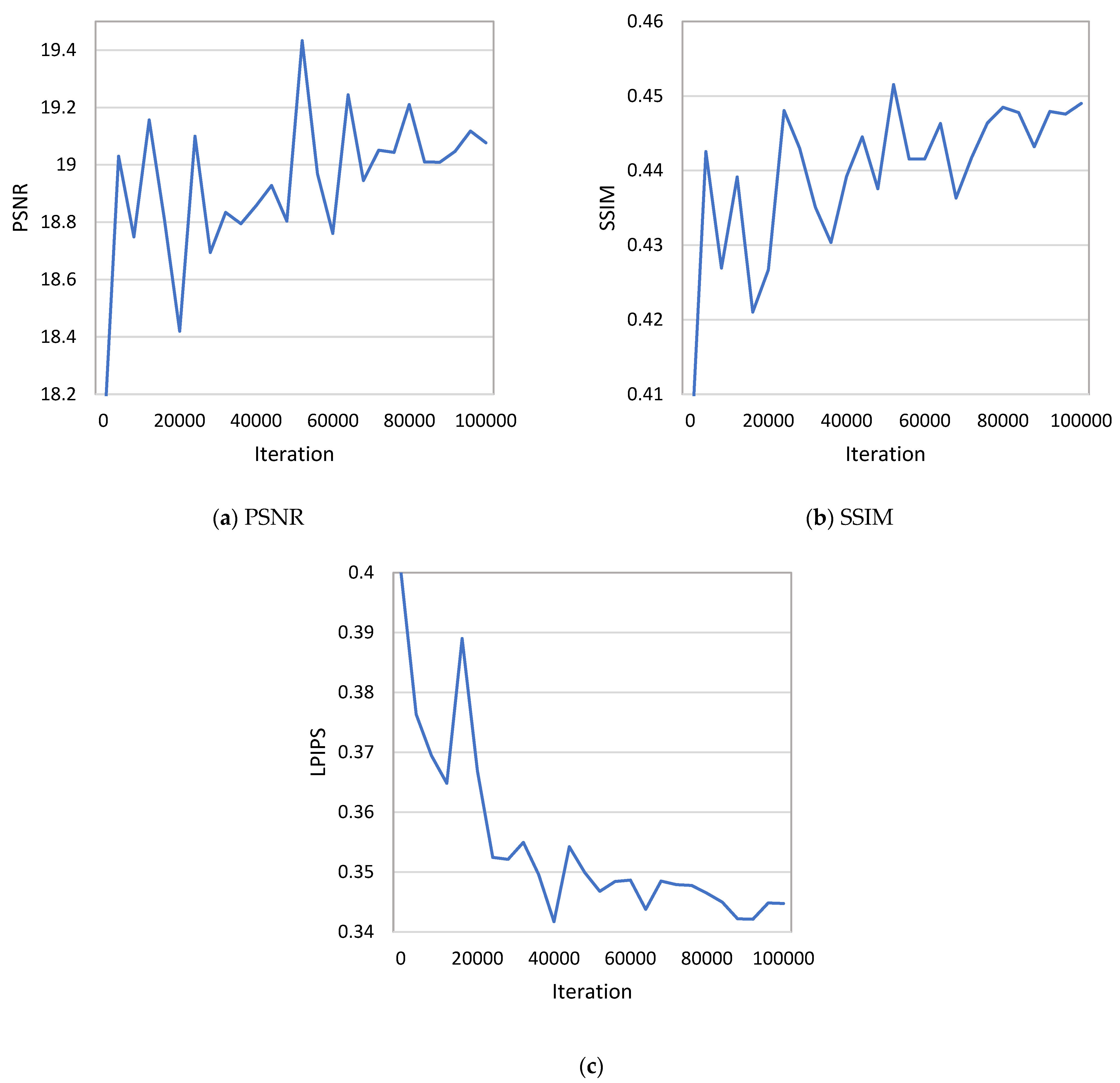
We saved the mean values of PSNR, SSIM and LPIPS for the validation dataset every 500 iterations while the model was trained and plotted them into three graphs for visual analysis.
Figure 3a shows the PSNR values during the training process. The horizontal coordinates are the number of iterations, and the vertical coordinates represent the PSNR values, from which we can observe that the oscillation amplitude of the PSNR values was very large at the beginning of the training period, and the difference between the highest and lowest peaks was more than 2. Our model gradually stabilised, and the amplitude stayed at around 0.2 when the number of iterations approached 100,000.
Figure 3b shows the curve of the SSIM value change during training, from which we can observe that the oscillation amplitude of the SSIM value was still very large at the beginning of training, and the difference between the highest peak and the lowest peak was more than 0.05. As the number of training iterations increased, the overall trend of the SSIM values gradually increased, the amplitude of oscillation gradually stabilised and the final amplitude remained around 0.01, which also indicates that our model gradually stabilises in the late training period.
Figure 3c shows the curve of the LPIPS value change during the training process. It shows that the quality of our model improved continuously as the number of training iterations increased, and the model stabilised and converged when the number of iterations approached 100,000.
4.5. Reconstruction Results Analysis of RHLAI Dataset
We conducted experiments using SRCNN [25], EDSR [29], SRGAN [34], ESRGAN [40], SPSR [42], Real-ESRGAN [52] and NDSRGAN on the RHLAI dataset, under the conditions where the training iterations, initial learning rates and training hardware environments were guaranteed to be the same.
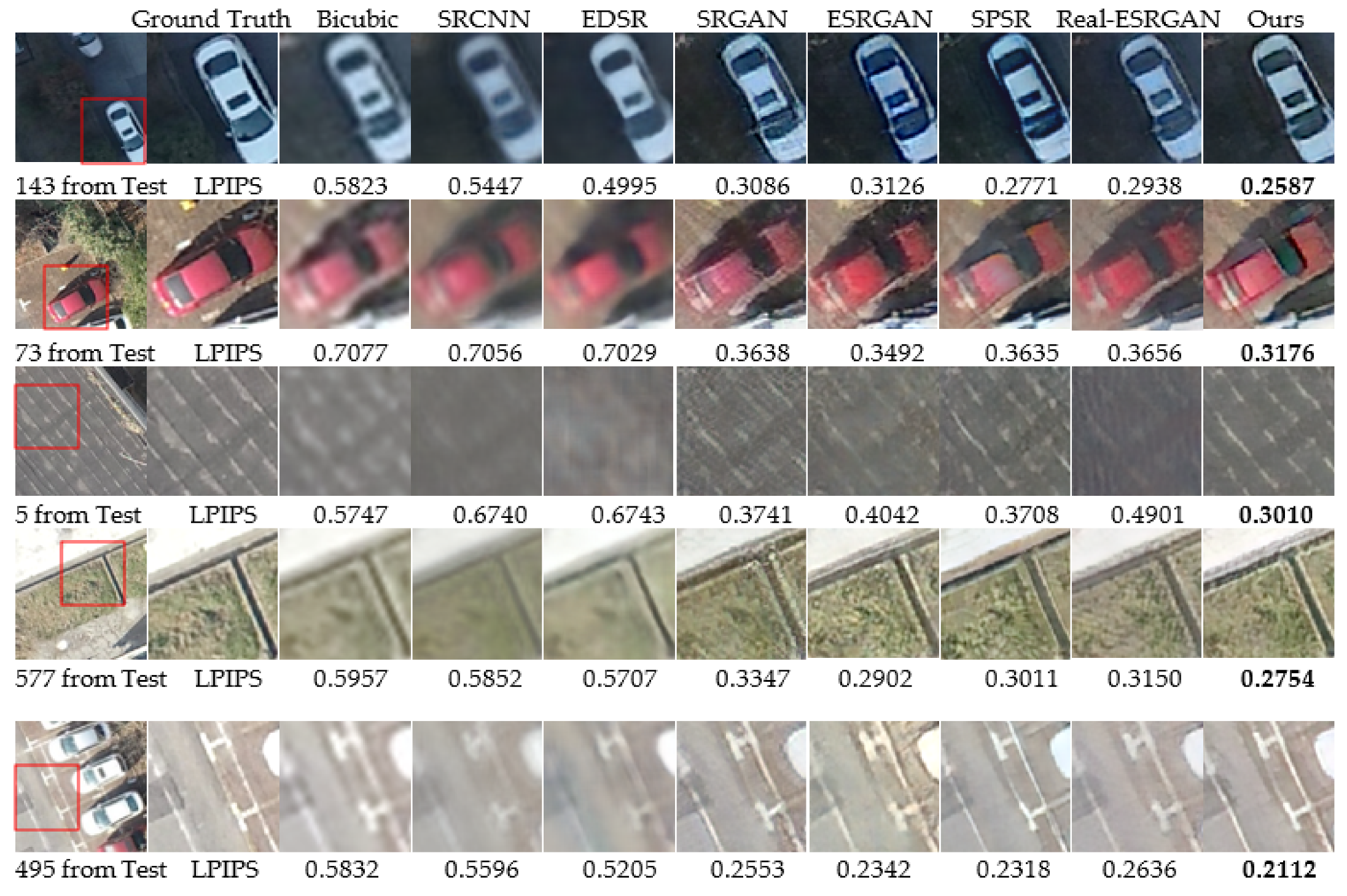
Table 3 shows the PSNR, SSIM and LPIPS values of the reconstructed images on the test dataset. Higher PSNR and SSIM values and lower LPIPS values represent better image quality. Through experimental comparison, we found that the bicubic interpolation methods and the CNN-based SR reconstruction methods tended to obtain higher PSNR and SSIM values compared with the GAN-based methods, but a large gap still exists between the real reconstruction visual effect and the GAN-based methods’ reconstruction effect, and the image visual effect is blurred (see Figure 4). Therefore, we believe that the PSNR and SSIM metrics do not represent the real image reconstruction quality well. The authors who developed ESRGAN [40] and SPSR [42] presented the same insights in their papers. For this reason, we calculated a metric closer to human visual perception, to continue the accuracy evaluation, namely LPIPS [51].Our model achieved the highest accuracy score, significantly exceeding the LPIPS value of the second-ranked SPSR model. It can be seen from Figure 4 that this metric is consistent with human visual perception. The lower the LPIPS value othe reconstructed image, the higher the reconstruction quality.
We also performed a group of qualitative and quantitative analyses of the reconstructed images in terms of human visual perception. Figure 4 shows that the reconstructed images from our model have richer texture details than the reconstructed images from other models, and the reconstructed images are closer to the real HR images.
The figure also shows that the images reconstructed using bicubic interpolation and CNN-based methods are obviously blurred, and the images reconstructed by the GAN-based methods are clearer.
As can be seen in the first and second rows of Figure 4, our model is able to reconstruct a clearer car outline. In the third row of Figure 4, our model is able to restore more of the white texture of the roof and produce fewer artifacts and in the fourth row of Figure 4, our model is able to generate a clearer gutter that is closer to the real HR image. In the fifth row of Figure 4, our model generates more regular and more detailed parking lines.
These results indicate that our model is able to take full advantage of the features of the original image and that the feature detail contours in the generated image are closer to the real HR image, due to the matrix mean discriminator utilised by NDSRGAN. The performance of NDSRGAN will be further discussed in Appendix A.
5. Discussion
To further demonstrate the good performance of NDSRGAN, we conducted a series of experiments using SRCNN, EDSR, SRGAN, ESGAN, SPSR, Real-ESRGAN and NDSRGAN on the DIV2K dataset [53], under conditions where the training iterations, initial learning rates and training hardware environments were guaranteed to be the same. Table 4 shows the PSNR, SSIM and LPIPS values of the reconstructed images in Set5 [54], Set14 [55] and Urban100 [56].
As can be seen in Table 4, the EDSR model obtained the highest PSNR and SSIM metrics in all three test sets. As described in Section 4.5, CNN-based models tended to obtain higher PSNR and SSIM values, but the image reconstruction visual results were not as good as those of the GAN-based models. The LPIPS metric is more consistent with human visual evaluation results, so the ranking of LPIPS values is more convincing regarding the superiority of the model. Our NDSRGAN model obtained the best LPIPS metrics in three test sets, further proving the superiority of our model’s reconstruction ability.
6. Conclusions
High-resolution aerial images are important in aerial photography applications, but they have a high acquisition cost and a long processing period. Moreover, the current models do not achieve a good reconstruction effect on real aerial image super-resolution reconstruction. Therefore, reconstructing high-quality high-resolution aerial images from real low-resolution aerial images is a great challenge.
To address the difficulty of reconstructing real aerial images by using existing super-resolution reconstruction models, we produced the RHLAI dataset with real aerial high- and low-resolution pairing for aerial image super-resolution reconstruction and proposed a new aerial image super-resolution reconstruction model called NDSRGAN.
We used multilevel dense connection to connect multiple dense connections in the residual dense block, so that the designed generative network could maximise the use of the features of real aerial images, and we used a matrix mean discriminator to optimise our discriminative network, which does not discriminate the whole image of the input but instead discriminates the input image locally in chunks.
The experimental results demonstrated that the reconstructed images obtained by image local discrimination were of higher quality and closer to the real high-resolution images. In our model, loss was used instead of the loss used in the mainstream models (ESRGAN [40], SPSR [42]), and this optimisation accelerated the convergence of the model, making it reach the global optimum faster.
The previous super-resolution reconstruction models and NDSRGAN were trained on the real aerial image dataset we produced, and the experiments showed that our proposed super-resolution reconstruction model for aerial images could reconstruct the real aerial images with better results, and that the reconstructed images achieved better results than previous methods regarding both quantitative metrics and qualitative evaluation.
Although the proposed method could reconstruct real aerial images with better results, the quality of the reconstructed images was not good when the model reconstructed images taken by different sensors. The lack of reconstruction generalisation ability of the super-resolution model on images taken by different sensors remains a problem that needs to be studied and addressed in the future.
Author Contributions
M.G. and Z.Z. proposed the network architecture design and the super-resolution framework. M.G. and H.L. performed the experiments and analysed the data. Z.Z. and H.L. wrote the paper. Y.H. revised the paper and provided valuable advice on the experiments. All authors have read and agreed to the published version of the manuscript.
Funding
This study was funded by the National Natural Science Foundation of China (41971356, 41701446) and the Open Fund of Key Laboratory of Urban Land Resources Monitoring and Simulation, Ministry of Natural Resources (KF-2020-05-011).
Institutional Review Board Statement
The study did not involve humans or animals.
Informed Consent Statement
The study did not involve humans.
Data Availability Statement
Not applicable.
Conflicts of Interest
The authors declare no conflict of interest.
Appendix A
In this section, we report the results of performing experimental analyses of model ablation, residual scaling factor size, discriminative matrix size of discriminator and image size of the input during model training.
Appendix A.1. Ablation Study
We performed stepwise improvement and optimisation on the base network of the ESRGAN model to prove that each part of our model optimisation was effective. We designed three comparative experiments.
The first was to add a multilevel densely connected network to the base generative network part to achieve multilevel information utilisation and feature fusion between multilevel DBs and DCRDBs. The second was to use a matrix mean discriminator instead of the original discriminator, in addition to the MDC. The third was our final network model, which uses in addition to MDC and MMD to compute the pixel loss and perceptual loss.
From the experimental results in Section 4.5, we concluded that PSNR and SSIM are not suitable for evaluating image quality, so we used only the LPIPS metric as the image quality assessment metric in the experiments discussed in the Appendix. The LPIPS values of the reconstructed images are shown in Table A1. After the MDC optimisation was added to the base network, the LPIPS value improved by 0.0065 compared with the base network, thereby proving that the MDC can effectively improve the image reconstruction ability of the network.

Table A1.
Mean value of LPIPS for different ablation experiments. Base represents the base network, MDC represents multilevel dense connection, MMD represents matrix mean discriminator and means that the pixel loss and perceptual loss are computed by loss. The best performance in bold.
Table A1.
Mean value of LPIPS for different ablation experiments. Base represents the base network, MDC represents multilevel dense connection, MMD represents matrix mean discriminator and means that the pixel loss and perceptual loss are computed by loss. The best performance in bold.
| Methods | |
|---|---|
| Base | |
| Base + MDC | |
| Base + MDC+ MMD | |
| Base + MDC + MMD + |
Meanwhile, after MMD was added, the LPIPS value of the reconstructed images significantly improved by 0.0236, which shows that MMD plays a crucial role in the optimisation of the model.
Finally, after the loss was added to the model, giving our final proposed SR reconstruction model NDSRGAN, the LPIPS value of the reconstructed images improved by 0.0184. From this result, we can conclude that our optimisation of the loss is also essential.
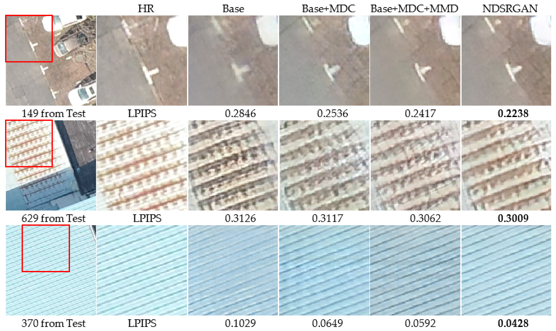
The reconstruction effects of each model in the above ablation experiments are shown in Figure A1. The first row of Figure A1 shows that the car parking lines in the reconstructed images of the base model are very blurred, which is directly related to the fact that the base model generative network does not make full use of the image features. After we added MDC optimisation to the generative network, the car parking lines in the reconstructed images became much clearer compared with those in base model, but the contours and colours of the parking lines still had some distortion. After we added MMD optimisation to the generative network optimisation, the contour of the parking line was significantly improved, and the colour of the parking line was closer to the original HR image. Finally, after we added loss optimisation to the model, the reconstructed parking lines became smoother, and the contour shape was closer to the original HR image.
Figure A1.
Reconstructed images of the ablation experiment and their corresponding LPIPS values. The best performance in bold.
Figure A1.
Reconstructed images of the ablation experiment and their corresponding LPIPS values. The best performance in bold.

From the second row of Figure A1, we can observe that the reconstructed images from the base model had serious colour distortion and obvious artifacts in the local zoomed images. After using MDC to optimise the generative network, we can see that the reconstructed image exhibited improved colour and fewer artifacts. When we optimised the discriminator with MMD, the colour of the reconstructed image was further corrected, and the overall image quality was improved. Finally, after we added loss optimisation, the final model reconstructed an image with the closest colour to the original HR image, the fewest artifacts and the best visual effect.
The third row of Figure A1 shows that the roof lines in the reconstructed images of the base model were rather blurred, and there was a serious loss of features. When the MDC-optimised generative network was used, the roof lines in the reconstructed images became clearer. After we used MMD to optimise the discriminator, the roof lines in the reconstructed image became clearer, but some colour distortion occurred. Finally, after we added the loss optimisation, the final reconstructed image had the sharpest roof line, and the colour was closer to the original HR image.
Appendix A.2. Residual Scaling Factor
In the MDC of the generative network, we used a residual scaling factor to set the feature information weights and we conducted group experiments by setting different residual scaling factors to select the most suitable residual scaling factor for the SR reconstruction of real aerial images. Preliminary experiments proved that when the residual scaling factor was larger than 0.4, the fusion of feature information was too redundant, and the model reconstructed the image poorly. Therefore, we chose the four residual scaling factors 0.1, 0.2, 0.3 and 0.4 to conduct the experiments.
The mean values of LPIPS on the test dataset are shown in Table A2. We can conclude from observation that when the residual scaling factor was 0.1, the LPIPS value of the reconstructed images was not the best, due to the loss of feature information in the process of MDC caused by a too-small residual scaling factor. When the residual scaling factor was 0.3 or 0.4, the LPIPS values of the reconstructed images became worse, compared with the value for a residual scaling factor of 0.2, because the residual scaling factor was too large. As a result, the feature information in the MDC process was too redundant, thereby negatively affecting the SR reconstruction of the image. When the residual scaling factor was 0.2, the LPIPS value mostly ranked first. This also shows that the reconstructed network can make the best use of the feature information in the multilevel densely connected network.
Table A2.
Mean value of LPIPS for models with different residual scaling factors, where represents the residual scaling factor. The best performance in bold.
Table A2.
Mean value of LPIPS for models with different residual scaling factors, where represents the residual scaling factor. The best performance in bold.
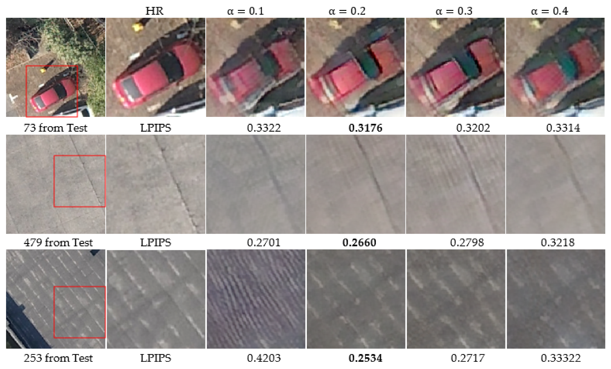
We also present the reconstructed images of the model trained with different residual scaling factors (Figure A2). From the first row of Figure A2, we can see that when the residual scaling factor was equal to 0.1, the overall visual effect of the red car was blurred due to the insufficient utilisation of feature information with a small residual scaling factor. When it was equal to 0.3, the reconstruction of the red car was too dark due to the feature redundancy caused by the large residual scaling factor. When it was equal to 0.4, the red car’s overall visual effect became worse and more blurred. When it was equal to 0.2, the reconstruction of the red car had the highest quality and was closest to the original HR image.
Figure A2.
Experimental results of the model corresponding to different residual scaling factors, where represents the residual scaling factor. The best performance in bold.
Figure A2.
Experimental results of the model corresponding to different residual scaling factors, where represents the residual scaling factor. The best performance in bold.

From the second row of Figure A2, we can observe that the reconstructed image of the roof surface was too smooth, and the features of the roof surface gaps were lost when the residual scaling factor was equal to 0.1. When the residual scaling factor was equal to 0.3, the roof surface was reconstructed with more artifacts. When the residual scaling factor was equal to 0.4, the overall reconstructed image was too smooth, and there was a serious loss of texture detail. When the residual scaling factor was equal to 0.2, the roof surface had the fewest artifacts, and the features were most fully preserved.
The third row of Figure A2 shows that the roof reconstruction effect was very poor when the residual scaling factor was equal to 0.1, and the features of the original HR image were not learned. When the residual scaling factor was equal to 0.3, the overall reconstructed image was blurred due to the redundancy of feature stacking. When the residual scaling factor was equal to 0.4, the overall roof reconstruction effect was even worse, and the features of the white lines of the original image were not learned. When the residual scaling factor was equal to 0.2, the roof white lines were better reconstructed, and the overall visual effect was closer to the original HR image.
Appendix A.3. Discriminative Matrix Size
To improve the discriminator’s ability to discriminate local features of an image, we used an MMD. The MMD aims to finally output a discriminative matrix to discriminate the image. Different discriminative matrices correspond to different receptive field sizes in the original image, and a large output discriminative matrix corresponds to a small receptive field for each value in the matrix in relation to the original image. We used different sizes of the discriminative matrix to perform group experiments to select the most suitable discriminative matrix size for SR reconstruction of aerial images. We set up three sets of comparison experiments with discriminative matrix sizes of 8 × 8, 14 × 14 and 19 × 19.
The mean values of the accuracy metric LPIPS for the reconstructed images are shown in Table A3, from which we find that the LPIPS value for the reconstructed images was not good when the discriminative matrix size was 8 × 8. When the size of the discriminative matrix was 19 × 19, the LPIPS of the reconstructed images ranked second, which shows that the discriminative matrix of size 19 × 19 was not the most suitable for the SR reconstruction of aerial images. When the discriminative matrix size was 14 × 14, the reconstructed images ranked first for the LPIPS metric, and therefore the experiments indicate that a discriminative matrix of size 14 × 14 was the most suitable choice for our SR reconstruction of real aerial images.
Table A3.
Mean value of LPIPS for models with different discriminative matrix sizes, where represents the size of the discriminative matrix. The best performance in bold.
Table A3.
Mean value of LPIPS for models with different discriminative matrix sizes, where represents the size of the discriminative matrix. The best performance in bold.
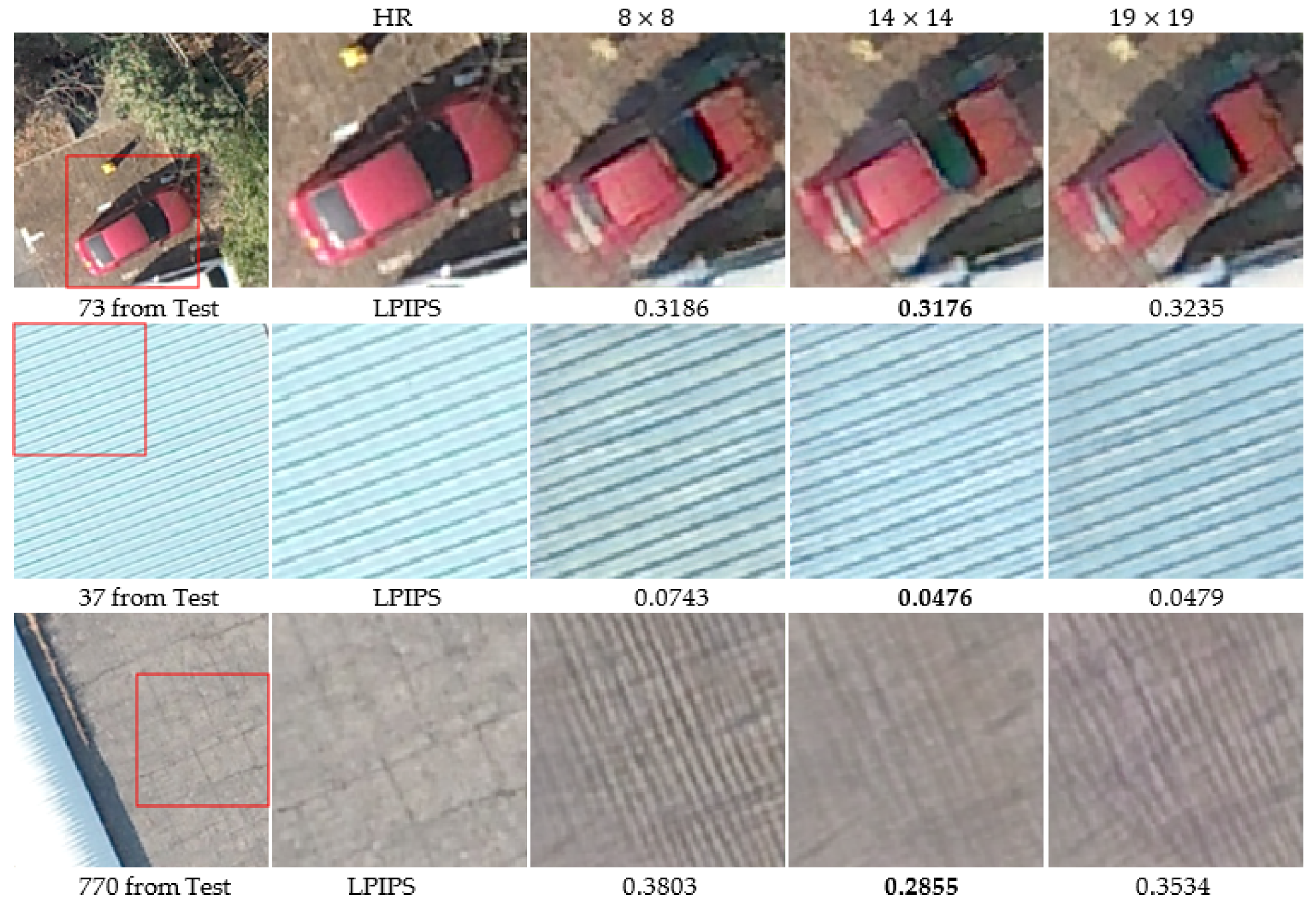
We also present the reconstructed images of the model trained with different discriminative matrix sizes (Figure A3). In the first row of Figure A3, when the discriminative matrix size was 8 × 8, the edges of the red car in the reconstructed image showed artifacts. When the discriminative matrix size was 19 × 19, the edges of the red car were very blurred and showed colour distortion. When the discriminative matrix size was 14 × 14, the edges of the red car were the most complete and showed the least distortion and fewest artifacts.
Figure A3.
Experimental results of models using different discriminative matrix sizes. The best performance in bold.
Figure A3.
Experimental results of models using different discriminative matrix sizes. The best performance in bold.

In the second row of Figure A3, when the discriminative matrix was of size 8 × 8, the overall colour of the roofline was dark and distorted. When the discriminative matrix was of size 19 × 19, the overall colour of the roofline was still dark, and some obvious white artifacts were observed. When the discriminative matrix was of size 14 × 14, the reconstructed image was closest to the original HR image.
In the third row of Figure A3, when the discriminative matrix was of size 8 × 8, the roof in the reconstructed image appears to show many artifacts. When the discriminative matrix was of size 19 × 19, the roof in the reconstructed image still appears to show more artifacts. When the discriminative matrix was of size 14 × 14, the roof in the reconstructed image produced the fewest artifacts and the best visual effect.
Appendix A.4. Random Crop Size of Training Input Images
In this section, we discuss the effect of the random crop size of the HR input images during model training on the reconstruction results of the model. We used three random crop sizes of 64 × 64, 128 × 128 and 192 × 192 for group comparison experiments to select the most suitable random crop size for SR reconstruction of aerial images.
The mean values of LPIPS for the reconstructed images are shown in Table A4, from which we can see that the reconstructed images did not obtain good LPIPS metric values at the random crop size of 64 × 64. At the random crop size of 192 × 192, the LPIPS metric on the reconstructed image ranked second, thus indicating that a random crop size of the training input image of 192 × 192 was not suitable for SR reconstruction of aerial images. For the random crop size of 128 × 128, the reconstructed images ranked first for the LPIPS metric. Therefore, we used a random crop size of 128 × 128 for SR reconstruction of real aerial images.
Table A4.
Mean value of LPIPS for models with different random crop sizes of input images, where represents the random crop size of training input images. The best performance in bold.
Table A4.
Mean value of LPIPS for models with different random crop sizes of input images, where represents the random crop size of training input images. The best performance in bold.
| . | |
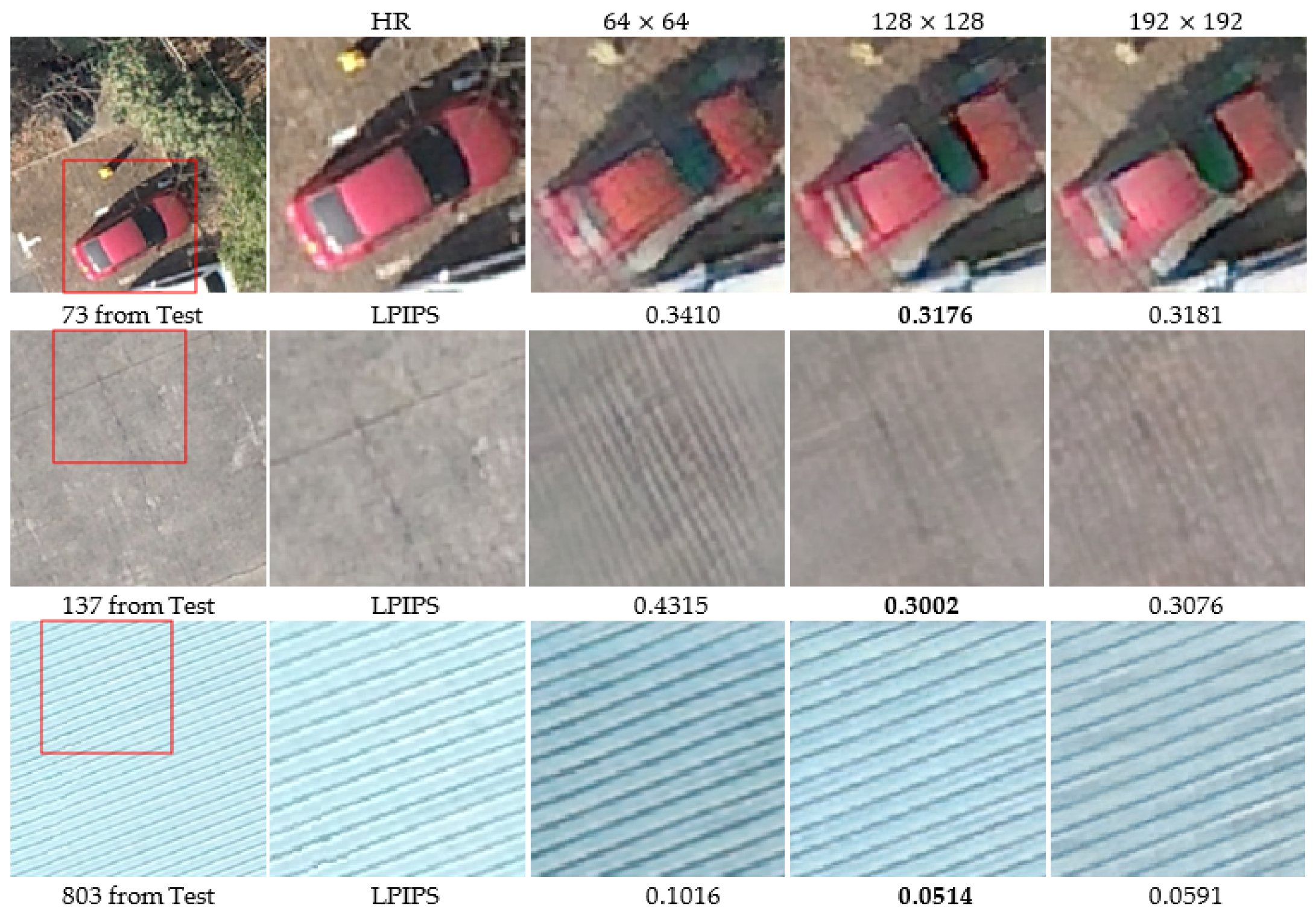
We present the reconstructed images of the model with different random crop sizes (Figure A4). The first row of Figure A4 shows that, for a crop size of 64 × 64, the red car in the reconstructed image was very blurred, and the reconstruction effect was poor. For a crop size of 192 × 192, the red car in the reconstructed image had some distortion. For a crop size of 128 × 128, the outline of the red car was the clearest, and the visual effect was closer to the original HR image.
Figure A4.
Reconstruction results with different random crop sizes. The best performance in bold.

In the second row of Figure A4, when the crop size was 64 × 64, more reconstruction artifacts were found on the roof surface in the reconstructed image. When the crop size was 192 × 192, many reconstruction artifacts remained on the roof surface in the reconstructed image. When the crop size was 128 × 128, the fewest reconstruction artifacts were found on the roof surface, and the best visual effect was achieved.
In the third row of Figure A4, when the crop size was 64 × 64, the colour of the blue roof in the reconstructed image was dark, and serious colour distortion occurred. For a crop size of 192 × 192, the colour of the blue roof in the reconstructed image was still dark, and some black artifact patches were found. When the crop size was 128 × 128, the colour and detail texture of the blue roof in the reconstructed image were closest to the original HR image, and the visual effect was the best.
References
- Walter, V. Automated GIS data collection and update. In Proceedings of the Photogrammetric Week′ 99, Heidelberg, Germany, 22–26 September 1999; pp. 267–280. [Google Scholar]
- Lee, K.; Ryu, H.Y. Automatic circuity and accessibility extraction by road graph network and its application with high-resolution satellite imagery. In Proceedings of the 2004 IEEE International Geoscience and Remote Sensing Symposium, Anchorage, AK, USA, 20–24 September 2004; Volume 5, pp. 3144–3146. [Google Scholar]
- Lim, S.B.; Seo, C.W.; Yun, H.C. Digital map updates with UAV photogrammetric methods. J. Korean Soc. Surv. Geod. Photogramm. Cartogr. 2015, 33, 397–405. [Google Scholar] [CrossRef]
- Guo, M.; Liu, H.; Xu, Y.; Huang, Y. Building Extraction Based on U-Net with an Attention Block and Multiple Losses. Remote Sens. 2020, 12, 1400. [Google Scholar] [CrossRef]
- Sun, H.; Sun, X.; Wang, H.; Li, Y.; Li, X. Automatic target detection in high-resolution remote sensing images using spatial sparse coding bag-of-words model. IEEE Geosci. Remote Sens. Lett. 2011, 9, 109–113. [Google Scholar] [CrossRef]
- Wu, F.; Duan, J.; Chen, S.; Ye, Y.; Ai, P.; Yang, Z. Multi-target recognition of bananas and automatic positioning for the inflorescence axis cutting point. Front. Plant Sci. 2021, 12, 705021. [Google Scholar] [CrossRef]
- Tang, Y.; Zhu, M.; Chen, Z.; Wu, C.; Chen, B.; Li, C.; Li, L. Seismic performance evaluation of recycled aggregate concrete-filled steel tubular columns with field strain detected via a novel mark-free vision method. Structures 2022, 37, 426–441. [Google Scholar] [CrossRef]
- Wang, Z.; Jiang, K.; Yi, P.; Han, Z.; He, Z. Ultra-dense GAN for satellite imagery super-resolution. Neurocomputing 2020, 398, 328–337. [Google Scholar] [CrossRef]
- Forsyth, D.; Ponce, J.; Mukherjee, S.; Bhattacharjee, A.K. Computer Vision: A Modern Approach; Prentice Hall: Upper Saddle River, NJ, USA, 2011. [Google Scholar]
- Huang, G.; Liu, Z.; van der Maaten, L.; Weinberger, K.Q. Densely Connected Convolutional Networks. In Proceedings of the 2017 IEEE Conference on Computer Vision and Pattern Recognition, Honolulu, HI, USA, 21–26 July 2017; pp. 2261–2269. [Google Scholar]
- Girshick, R. Fast R-CNN. In Proceedings of the IEEE International Conference on Computer Vision, Santiago, Chile, 7–13 December 2015; pp. 1440–1448. [Google Scholar]
- Koester, E.; Sahin, C.S. A comparison of super-resolution and nearest neighbors interpolation applied to object detection on satellite data. arXiv 2019, arXiv:1907.05283. [Google Scholar]
- Zhang, X. A new kind of super-resolution reconstruction algorithm based on the ICM and the bilinear interpolation. In Proceedings of the 2008 International Seminar on Future BioMedical Information Engineering, Wuhan, China, 18 December 2008; pp. 183–186. [Google Scholar]
- Zhang, X. A new kind of super-resolution reconstruction algorithm based on the ICM and the bicubic interpolation. In Proceedings of the 2008 International Symposium on Intelligent Information Technology Application Workshops, Shanghai, China, 21–22 December 2008; pp. 817–820. [Google Scholar]
- Gilman, A.; Bailey, D.G. Near optimal non-uniform interpolation for image super-resolution from multiple images. Image Vis. Comput. N. Z. Great Barrier Isl. N. Z. 2006, 20, 31–35. [Google Scholar]
- Rasti, P.; Demirel, H.; Anbarjafari, G. Iterative back projection based image resolution enhancement. In Proceedings of the 2013 8th Iranian Conference on Machine Vision and Image Processing, Zanjan, Iran, 10–12 September 2013; pp. 237–240. [Google Scholar]
- Tipping, M.E.; Bishop, C.M. Bayesian image super-resolution. In Proceedings of the Advances in Neural Information Processing Systems, Vancouver and Whistler, BC, Canada, 8–13 December 2003; pp. 1303–1310. [Google Scholar]
- Fan, C.; Wu, C.; Li, G.; Ma, J. Projections onto convex sets super-resolution reconstruction based on point spread function estimation of low-resolution remote sensing images. Sensors 2017, 17, 362. [Google Scholar] [CrossRef]
- Xu, J.; Gao, Y.; Xing, J.; Fan, J.; Gao, Q.; Tang, S. Two-direction self-learning super-resolution propagation based on neighbor embedding. Signal Process. 2021, 183, 108033. [Google Scholar] [CrossRef]
- Zhang, J.; Shao, M.; Yu, L.; Li, Y. Image super-resolution reconstruction based on sparse representation and deep learning. Signal Process. Image Commun. 2020, 87, 115925. [Google Scholar] [CrossRef]
- Ooi, Y.K.; Ibrahim, H. Deep Learning Algorithms for Single Image Super-Resolution: A Systematic Review. Electronics 2021, 10, 867. [Google Scholar] [CrossRef]
- Minsky, M. Steps toward Artificial Intelligence. Proc. IRE 1961, 49, 8–30. [Google Scholar] [CrossRef]
- Yang, W.; Zhang, X.; Tian, Y.; Wang, W.; Xue, J.; Liao, Q. Deep Learning for Single Image Super-Resolution: A Brief Review. IEEE Trans. Multimed. 2019, 21, 3106–3121. [Google Scholar] [CrossRef] [Green Version]
- Dong, C.; Loy, C.C.; He, K.; Tang, X. Image super-resolution using deep convolutional networks. IEEE Trans. Pattern Anal. 2015, 38, 295–307. [Google Scholar] [CrossRef] [PubMed] [Green Version]
- LeCun, Y.; Boser, B.; Denker, J.S.; Henderson, D.; Howard, R.E.; Hubbard, W.; Jackel, L.D. Backpropagation Applied to Handwritten Zip Code Recognition. Neural Comput. 1989, 1, 541–551. [Google Scholar] [CrossRef]
- Dong, C.; Loy, C.C.; Tang, X. Accelerating the super-resolution convolutional neural network. In Proceedings of the European Conference on Computer Vision, Amsterdam, The Netherlands, 8–16 October 2016; pp. 391–407. [Google Scholar]
- Xu, L.; Ren, J.S.; Liu, C.; Jia, J. Deep Convolutional Neural Network for Image Deconvolution. In Proceedings of the Advances in Neural Information Processing Systems, Montreal, QC, Canada, 8–13 December 2014; pp. 1790–1798. [Google Scholar]
- He, K.; Zhang, X.; Ren, S.; Sun, J. Deep Residual Learning for Image Recognition. In Proceedings of the IEEE Conference on Computer Vision and Pattern Recognition, Las Vegas, NV, USA, 27–30 June 2016; Volume abs/1512.03385, pp. 770–778. [Google Scholar]
- Lim, B.; Son, S.; Kim, H.; Nah, S.; Mu Lee, K. Enhanced deep residual networks for single image super-resolution. In Proceedings of the IEEE Conference on Computer Vision and Pattern Recognition Workshops, Honolulu, HI, USA, 21–26 July 2017; pp. 136–144. [Google Scholar]
- Ioffe, S.; Szegedy, C. Batch Normalization: Accelerating Deep Network Training by Reducing Internal Covariate Shift. arXiv 2015, arXiv:1502.03167. [Google Scholar]
- Xiaomei, Y.; Chenghu, Z. Analysis of the complexity of remote sensing image and its role on image classification. In Proceedings of the IEEE Geoscience and Remote Sensing Symposium, Honolulu, HI, USA, 24–28 July 2000; Volume 5, pp. 2179–2181. [Google Scholar]
- Aumann, R.; Brandenburger, A. Epistemic Conditions for Nash Equilibrium. Econometrica 1995, 63, 1161–1180. [Google Scholar] [CrossRef]
- Goodfellow, I.J.; Pouget-Abadie, J.; Mirza, M.; Xu, B.; Warde-Farley, D.; Ozair, S.; Courville, A.; Bengio, Y. Generative adversarial networks. In Proceedings of the Advances in Neural Information Processing Systems, Montreal, QC, Canada, 8–13 December 2014; pp. 2672–2680. [Google Scholar]
- Ledig, C.; Theis, L.; Huszár, F.; Caballero, J.; Cunningham, A.; Acosta, A.; Aitken, A.; Tejani, A.; Totz, J.; Wang, Z. Photo-realistic single image super-resolution using a generative adversarial network. In Proceedings of the IEEE Conference on Computer Vision and Pattern Recognition, Honolulu, HI, USA, 21–26 July 2017; pp. 4681–4690. [Google Scholar]
- Clements, M.P.; Hendry, D.F. On the limitations of comparing mean square forecast errors. J. Forecast. 1993, 12, 617–637. [Google Scholar] [CrossRef]
- Gatys, L.A.; Ecker, A.S.; Bethge, M. Texture synthesis and the controlled generation of natural stimuli using convolutional neural networks. In Proceedings of the Bernstein Conference 2015, Heidelberg, Germany, 15–17 September 2015. [Google Scholar]
- Bruna, J.; Sprechmann, P.; Lecun, Y. Super-Resolution with Deep Convolutional Sufficient Statistics. In Proceedings of the International Conference on Learning Representations, San Juan, Puerto Rico, 2–4 May 2016; pp. 1–17. [Google Scholar]
- Johnson, J.; Alahi, A.; Fei-Fei, L. Perceptual Losses for Real-Time Style Transfer and Super-Resolution. In Proceedings of the European Conference on Computer Vision, Amsterdam, The Netherlands, 8–16 October; pp. 694–711.
- Simonyan, K.; Zisserman, A. Very Deep Convolutional Networks for Large-Scale Image Recognition. In Proceedings of the International Conference on Learning Representations, Banff, AB, Canada, 14–16 April 2014; pp. 1–14. [Google Scholar]
- Wang, X.; Yu, K.; Wu, S.; Gu, J.; Liu, Y.; Dong, C.; Qiao, Y.; Change Loy, C. Esrgan: Enhanced super-resolution generative adversarial networks. In Proceedings of the European Conference on Computer Vision Workshops, Munich, Germany, 8–14 September 2018; pp. 1–16. [Google Scholar]
- Jolicoeur-Martineau, A. The relativistic discriminator: A key element missing from standard GAN. In Proceedings of the International Conference on Learning Representations, Vancouver, BC, Canada, 30 April–3 May 2018; pp. 1–25. [Google Scholar]
- Ma, C.; Rao, Y.; Cheng, Y.; Chen, C.; Lu, J.; Zhou, J. Structure-Preserving Super Resolution With Gradient Guidance. In Proceedings of the 2020 IEEE/CVF Conference on Computer Vision and Pattern Recognition, Seattle, WA, USA, 13–19 June 2020; pp. 7766–7775. [Google Scholar]
- Szegedy, C.; Ioffe, S.; Vanhoucke, V.; Alemi, A. Inception-v4, inception-resnet and the impact of residual connections on learning. In Proceedings of the AAAI Conference on Artificial Intelligence, San Francisco, CA, USA, 4–9 February 2017; Volume 31, pp. 1–7. [Google Scholar]
- Xu, B.; Wang, N.; Chen, T.; Li, M. Empirical evaluation of rectified activations in convolutional network. arXiv 2015, arXiv:1505.00853. [Google Scholar]
- Maas, A.L.; Hannun, A.Y.; Ng, A.Y. Rectifier nonlinearities improve neural network acoustic models. In Proceedings of the 30th International Conference on Machine Learning, Atlanta, GA, USA, 16–21 June 2013; Volume 30, p. 3. [Google Scholar]
- Isola, P.; Zhu, J.Y.; Zhou, T.; Efros, A.A. Image-to-Image Translation with Conditional Adversarial Networks. In Proceedings of the IEEE conference on computer vision and pattern recognition, Honolulu, HI, USA, 21–26 July 2017; Volume abs/1611.07004, pp. 1125–1134. [Google Scholar]
- Long, J.; Shelhamer, E.; Darrell, T. Fully convolutional networks for semantic segmentation. In Proceedings of the IEEE Conference on Computer Vision and Pattern Recognition, Boston, MA, USA, 7–12 June 2015; pp. 3431–3440. [Google Scholar]
- Kingma, D.P.; Ba, J. Adam: A Method for Stochastic Optimization. In Proceedings of the International Conference on Learning Representations, San Diego, CA, USA, 7–9 May 2015; pp. 1–15. [Google Scholar]
- Yang, C.; Ma, C.; Yang, M. Single-Image Super-Resolution: A Benchmark. In Proceedings of the European Conference on Computer Vision, Zurich, Switzerland, 6–12 September 2014; pp. 372–386. [Google Scholar]
- Zhou, W.; Bovik, A.C.; Sheikh, H.R.; Simoncelli, E.P. Image quality assessment: From error visibility to structural similarity. IEEE Trans. Image Process. 2004, 13, 600–612. [Google Scholar]
- Zhang, R.; Isola, P.; Efros, A.A.; Shechtman, E.; Wang, O. The Unreasonable Effectiveness of Deep Features as a Perceptual Metric. In Proceedings of the IEEE Conference on Computer Vision and Pattern Recognition, Salt Lake City, UT, USA, 18–23 June 2018; pp. 586–595. [Google Scholar]
- Wang, X.; Xie, L.; Dong, C.; Shan, Y. Real-esrgan: Training real-world blind super-resolution with pure synthetic data. In Proceedings of the IEEE/CVF International Conference on Computer Vision, Montreal, BC, Canada, 11–17 October 2021; pp. 1905–1914. [Google Scholar]
- Agustsson, E.; Timofte, R. Ntire 2017 challenge on single image super-resolution: Dataset and study. In Proceedings of the IEEE conference on computer vision and pattern recognition workshops, Honolulu, HI, USA, 21–26 July 2017; pp. 126–135. [Google Scholar]
- Bevilacqua, M.; Roumy, A.; Guillemot, C.; Alberi-Morel, M.L. Low-complexity single-image super-resolution based on nonnegative neighbor embedding. In Proceedings of the British Machine Vision Conference, Surrey, UK, 3–7 September 2012. [Google Scholar]
- Zeyde, R.; Elad, M.; Protter, M. On single image scale-up using sparse-representations. In Proceedings of the International Conference on Curves and Surfaces, Avignon, France, 24–30 June 2010; pp. 711–730. [Google Scholar]
- Huang, J.; Singh, A.; Ahuja, N. Single image super-resolution from transformed self-exemplars. In Proceedings of the IEEE Conference on Computer Vision and Pattern Recognition, Boston, MA, USA, 7–12 June 2015; pp. 5197–5206. [Google Scholar]
Figure 1.
Network structure of NDSRGAN. represents LR images and represents the image generated by the generative network. represents the convolutional layer. represents the u-th DCRDB module. denotes the upsampling network. represents the original HR image and represents the output image of the generative network. In addition, k represents the convolution kernel size, c represents the number of convolution kernels and s represents stride. The arrows in the figure represent the flow of the feature map.

Figure 2.
Internal structure of DCRDB and DB. (a) Internal structure of DCRDB. represents the v-th dense block. represents the convolutional layer. (b) Internal structure of DB. represents the w-th CL module. The CL module consists of a convolutional layer and a LReLU layer. represents the convolutional layer. The arrows in the figure represent the flow of the feature map.

Figure 3.
Three metric-value curves for NDSRGAN with increasing numbers of training iterations. (a) PSNR; (b) SSIM; (c) LPIPS.
Figure 3.
Three metric-value curves for NDSRGAN with increasing numbers of training iterations. (a) PSNR; (b) SSIM; (c) LPIPS.

Figure 4.
Visualisation effects of reconstructed images by different methods and their corresponding LPIPS values. The best performance in bold.
Figure 4.
Visualisation effects of reconstructed images by different methods and their corresponding LPIPS values. The best performance in bold.

Table 1.
The size of the output matrix of each layer of the network, where represents the size of the input image, represent the sizes of each convolution kernel from the first layer to the fifth layer, represent the amounts of padding from the first layer to the fifth layer, represent the sizes of each convolutional step from the first layer to the fifth layer, represent the sizes of the output matrix from the first layer to the fourth layer and represents the size of the final output matrix from the discriminator.
| Network Layers | Calculation Formula | Size of the Output Matrix |
|---|---|---|
| the first layer | ||
| the second layer | ||
| the third layer | ||
| the fourth layer | ||
| the fifth layer |
Table 2.
Mean values of PSNR, SSIM and LPIPS for cross-validation. The best performance in bold.
| PSNR | |||||||||
| SSIM | |||||||||
| LPIPS |
Table 3.
Mean values of PSNR, SSIM and LPIPS for different methods. The best performance in bold.
| Metrics | Bicubic | CNN | GAN | |||||
|---|---|---|---|---|---|---|---|---|
| SRCNN | EDSR | SRGAN | ESRGAN | SPSR | Real-ESRGAN | Ours | ||
| PSNR | ||||||||
| SSIM | ||||||||
| LPIPS | ||||||||
Table 4.
Mean values of PSNR, SSIM and LPIPS for different methods in Set5, Set14 and Urban100. The best performance in bold.
Publisher’s Note: MDPI stays neutral with regard to jurisdictional claims in published maps and institutional affiliations. |
© 2022 by the authors. Licensee MDPI, Basel, Switzerland. This article is an open access article distributed under the terms and conditions of the Creative Commons Attribution (CC BY) license (https://creativecommons.org/licenses/by/4.0/).
Share and Cite
MDPI and ACS Style
Guo, M.; Zhang, Z.; Liu, H.; Huang, Y. NDSRGAN: A Novel Dense Generative Adversarial Network for Real Aerial Imagery Super-Resolution Reconstruction. Remote Sens. 2022, 14, 1574. https://doi.org/10.3390/rs14071574
AMA Style
Guo M, Zhang Z, Liu H, Huang Y. NDSRGAN: A Novel Dense Generative Adversarial Network for Real Aerial Imagery Super-Resolution Reconstruction. Remote Sensing. 2022; 14(7):1574. https://doi.org/10.3390/rs14071574
Chicago/Turabian StyleGuo, Mingqiang, Zeyuan Zhang, Heng Liu, and Ying Huang. 2022. "NDSRGAN: A Novel Dense Generative Adversarial Network for Real Aerial Imagery Super-Resolution Reconstruction" Remote Sensing 14, no. 7: 1574. https://doi.org/10.3390/rs14071574
Note that from the first issue of 2016, this journal uses article numbers instead of page numbers. See further details here.