Technical Note

Microburst, Windshear, Gust Front, and Vortex Detection in Mega Airport Using a Single Coherent Doppler Wind Lidar

1
School of Earth and Space Science, University of Science and Technology of China, Hefei 230026, China
2
ZhongKe-YiAn Technology Co., Ltd., Shenzhen 518066, China
3
Meteorological Center of Southwest Air Traffic Management Bureau of CAAC, Chengdu 610202, China
4
Tibet Autonomous Region Administration of CAAC, Lhasa 850707, China
5
North China Regional Air Traffic Management Bureau of CAAC, Beijing 102604, China
*
Author to whom correspondence should be addressed.
Remote Sens. 2022, 14(7), 1626; https://doi.org/10.3390/rs14071626
Submission received: 28 January 2022 / Revised: 24 March 2022 / Accepted: 24 March 2022 / Published: 28 March 2022

Abstract

:
Accurate wind shear detection is crucial for aviation safety, especially in landing and departure. A new approach for windshear alerting is proposed and demonstrated. This approach monitors orthogonal wind components in multiple runways using single coherent Doppler wind lidar (CDWL). First, the two orthogonal components of the wind field are retrieved from radial speed by an updated variational method. Then, the heading wind and cross wind on different runways are calculated simultaneously, without the location restriction of the single lidar. Finally, a windshear alerting message is generated through quantitatively evaluating the distribution of shear ramps over the monitoring area. The new CDWL-based approach for windshear alerting is implemented at the Beijing Daxing International Airport. The retrieved horizontal wind from the lidar is consistent with that from anemometers. Thanks to its high spatial/temporal resolution, some meteorological phenomena of aviation hazards, including microburst, windshear, gust front, and vortex are well captured. Particularly, all 10 windshear cases reported by crews are successfully identified during the windshear verification experiment, demonstrating the effectiveness and robustness of the new approach.

1. Introduction

Low-level wind shear refers to a sudden, drastic change in wind speed or wind direction in the atmosphere, occurring within 600 m above ground level [1]. Encountering wind shear will cause an instantaneous change in the aircraft airspeed, which will lead to a change in the aircraft lift and deviation from the intended flight path, thereby threatening the flight safety of civil aircraft [2]. In recent years, airport wind shear accidents have often been reported, especially in take-off and landing processes [3,4,5]. With the rapid growth in global aviation transportation, it is urgent to improve the ability of detecting, identifying, alerting, and forecasting windshear to ensure the safety, regularity, and efficiency of flight operations [6].
The Terminal Doppler Weather Radar (TDWR) network [7] and the Low-Level Windshear Alert System (LLWAS) system consist of several anemometers installed in the vicinity of runways that have previously been applied in low-level wind shear monitoring for airports [8]. Moreover, balloon soundings, wind profilers [9], ground-based weather radar, lidar, and MET satellites are also adopted in windshear detection [1]. Among these instruments, the coherent Doppler wind lidar (CDWL) is a promising wind detection instrument that provides flexible scanning with high temporal and spatial resolutions. It can cooperate with radar to provide full weather condition detection.
The CDWL has been widely used in different areas, such as the detection of the atmosphere boundary layer [10,11,12], gravity waves [13], turbulence [14,15], windshear [2,16,17], gust [18], and aircraft vortex [19]. Detection and identification of low-level wind shear using CDWL has become a popular topic of research in aviation [3,5,20,21,22,23]. The Doppler lidar system installed at the Hong Kong International Airport (HKIA) has been applied for wind shear alerting since 2002. Comprehensive studies on wind shear events observed by the lidar have been conducted at HKIA, including the design of the glide path scanning and the development of an automatic wind shear detection algorithm [4,14,24,25,26,27,28,29]. Besides HKIA, lidar systems for wind shear detection have been tested at several international airports, such as Narita International Airport [30], Bratislava Airport [20], Lanzhou Zhongchuan International Airport [5], Beijing Capital International Airport [3], and others [21,22]. The headwind profile of a single runway can be synthesized from the radial velocity in line with the glide path [28], while it is difficult to be applied to a mega airport (an airport with multiple runways) due to the requirement of multiple lidars and their limited locations. Deploying multiple lidars has double costs: it increases the difficulty and efforts of instrument maintenance and data assembly. Retrieval of a horizontal 2D wind field is a challenge with single lidar [31], and it is difficult to apply to wind shear alerting due to the lack of quantitative, accurate, and efficient methods for evaluating wind shear intensity.
In this paper, a new approach using a single CDWL is presented for windshear alerting for multiple runways, through quantitatively evaluating the distribution of shear ramps based on orthogonal wind components. The CDWL system achieves monitor four runways in a detection range of 13 km, providing services for aviation safety at Beijing Daxing International Airport (BDIA). The approach requires enough detection range to cover multiple runways. The degree of air cleanliness, low clouds, low atmospheric visibility, gross air pollution, and extreme weather conditions will lead to a short lidar detection range. In these cases, multiple lidars are usually needed to cover the whole area of a mega-airport to implement this approach. This paper is organized as follows: the wind retrieval and windshear alerting method are introduced in Section 2. The results of windshear, microburst, and vortex structures with alerting information in the field experiment are described in Section 3. Finally, a conclusion is drawn in Section 4.

2. Windshear Evaluation Method

The diagrams of coordinates and velocities are shown in Figure 1. The headwind of runway A can be constructed directly with the radial speed by glide path scanning [28], for location of the lidar is close to the runway. However, it is not applicable to runway B, where the angle between the radial velocity and the headwind is large. In this case, 2D wind components are required to obtain the head wind.
The observed radial speed V o can be obtained accurately by the lidar with PPI scanning. Then, the tangential speed V t is the key value to be retrieved. At low elevation angles, the radial speed and tangential speed can be expressed as:
V r = u c o s θ + v s i n θ
V t = u sin θ + v cos θ
where u and v are the two components of velocity in the lidar coordinate system x o y . θ is the azimuth angle, with 0° corresponding to the north. Differentiating Equation (1) along the azimuth direction can be written as:
V r θ = u s i n θ + v c o s θ + u θ c o s θ + v θ s i n θ
Combining Equation (2) and Equation (3), we can obtain
V t = V r θ u θ c o s θ v θ s i n θ
A variational method is adopted to retrieve the u and v based on the observed radial speed. The cost function of the variational method is defined as:
J = J b + J r + J t + J e
where
J b = i , j W b [ ( u u b ) 2 + ( v v b ) 2 ]
J r = i , j W r ( V o V r ) 2
J t = i , j W t ( u s i n θ + v c o s θ V o θ + u θ c o s θ + v θ s i n θ ) 2
J e = i , j W e [ d 2 ( u x + v y ) + d 2 ( v x u y ) + d 2 ( 2 u + 2 v ) ]
J b , J r , and J t are the background term, the radial speed term, and the tangential speed term, respectively. u b and v b are obtained by minimizing the cost function, when W b = 0 . J e is the smoothing term involving the divergence, vorticity, and Laplacian; d = 30   m is the grid size in the retrieval field. The weighting coefficients are taken as W r = 1   ( m 2 s 2 ) , W t = 0.5   ( m 2 s 2 ) , and W b = W e = 0.1   ( m 2 s 2 ) [32], which are empirically chosen to ensure that the constraints have proper orders of magnitude. u and v are expanded in terms of second order Legendre polynomials, as recommended by [32,33]. Compared with previous works [32,33], the J t is added as a measurement of the retrieved tangential speed.
Using Equation (2), the tangential speed V t can be obtained using u and v retrieved by the variational method. By taking full advantage of the observed radial speed V o , the retrieved two component winds can be updated by:
u = V o c o s θ V t s i n θ
v = V o s i n θ + V t c o s θ
The center of the runway ( x k o , y k o ) is set as the origin O k , the direction parallel to the runway is set as the X k axis, and the direction perpendicular to the runway is set as the Y k axis. Then, the heading wind, U k , and crossing wind, V k , in the runway coordinates X k O k Y k are expressed as:
U k = u c o s θ k + v s i n θ k
V k = u s i n θ k + v c o s θ k
where θ k is the angle between the runway coordinate and the lidar coordinate. The position measuring points are written as:
X k = ( x x k o ) c o s θ k + ( y y k o ) s i n θ k
Y k = ( x x k o ) s i n θ k + ( y y k o ) c o s θ k
The change in wind speed during take-off and landing is the point of focus. “Windshear” is exclusively defined as wind change along the glide path. The magnitude of such “windshear” will be expressed in terms of velocity difference (in m/s), following the established practice in provision of alerts to aviation users [1,4]. The windshear usually has the characteristics of sudden and rapid changes. Identifying wind shear with a single head profile is likely to result in missing a report. In this work, the wind speed differences between any two measuring points in the monitoring area are calculated and recorded to evaluate the intensity level of the windshear.
Windshear alerting is applied to operations in the airport vicinity within 3 nautical miles (NM) of the point of landing or departure along the intended flight path, as recommended by the ICAO [1]. The monitoring area of runway k is set as:
{ ( 3 m + L k 2 ) < X k < ( 3 m + L k 2 ) , m 2 < Y k < m 2 }
where m is the unit length, which is set as 1.852 km (1 NM). The heading wind change of any two points A and B in the monitoring along the glide path are calculated as
W a , b = U a U b
The severity factor I a , b is used to describe the intensity of the windshear, which is calculated as [34,35,36]
I a , b = | W a , b / L a , b 1 / 3 | 3 / V a p p
L a , b = [ ( X k a X k b ) 2 + ( Y k a Y k b ) 2 ] 1 / 2
where V a p p and L a , b are the approach speed of the aircraft and the windshear ramp length, respectively. W a , b / L a , b 1 / 3 is the change rate of wind speed. I a , b is used to remove the gentle windshear ramp, which changes slowly in length. The filtered windshear ramp is recorded as [ W a , b , ( X k a + X k b ) / 2 ] .
Finally, the distribution of the windshear center on the runway coordinate is obtained. The monitoring area is separated into 7 subareas by 1.852 km. The number of shear ramps in each subarea is counted. When the number of shear centers in the subarea is greater than the specified threshold, a windshear alert message is generated. The windshear alert message contains detailed information, including runway (identification of the runway and specification of approach or departure corridor), character (microburst, wind shear or gust front), magnitude (change in the wind speed, loss or gain), and the subarea [20]. By making full use of the data scanned by PPI, the windshear can be well evaluated and captured. In addition, the error and outlier interference of the wind data can be reduced through the statistics of wind shear in the monitoring area in this work.

3. Experiment and Result

The field experiment was performed at BDIA, China (39°29′N, 116°24′E), from 1 April to 1 September 2021. BDIA is the second international airport of Beijing along with Beijing Capital International Airport. For the time being, the mega-airport has four runways, as shown in Figure 2a. The runways are marked as 17R/35L, 17L/35R, 11L/29R, and 01L/19R, respectively. As flights continue to grow, windshear alerting services are becoming increasingly important.
A compact and integrated micro-pulse CDWL was applied at the airport, as shown in Figure 2b. It has worked continuously in different weather conditions since 1 April 2021. The CDWL is operated at an eye-safe wavelength of 1.5 μm. The spatial and temporal resolution are 30 m and 0.2 s of each beam, respectively. The key parameters are listed in Table 1. The CDWL supports multiple scanning patterns, including plan position indicator (PPI), range height indicator (RHI), velocity azimuth display (VAD), glide path (GP), and custom defined pattern. The updated CDWL system has made a lot of improvements and optimization, and its reliability has been verified in previous works [2,12,13]. During this experiment, the lidar mainly operated in the PPI scanning mode with a period of about 40 s. The scanning range of azimuth was set as 150° to 360° due to obstacles behind it. Elevation angles were set as 0° to 7° with steps of 1°, to cover the runway and glide path. Continuous verification of windshear alerting was conducted from 1 April to 6 June—a total of 66 days—until 10 pilot reports were accumulated. Continuous verification of wind retrieval was conducted for 87 days, from 6 June to 31 August.

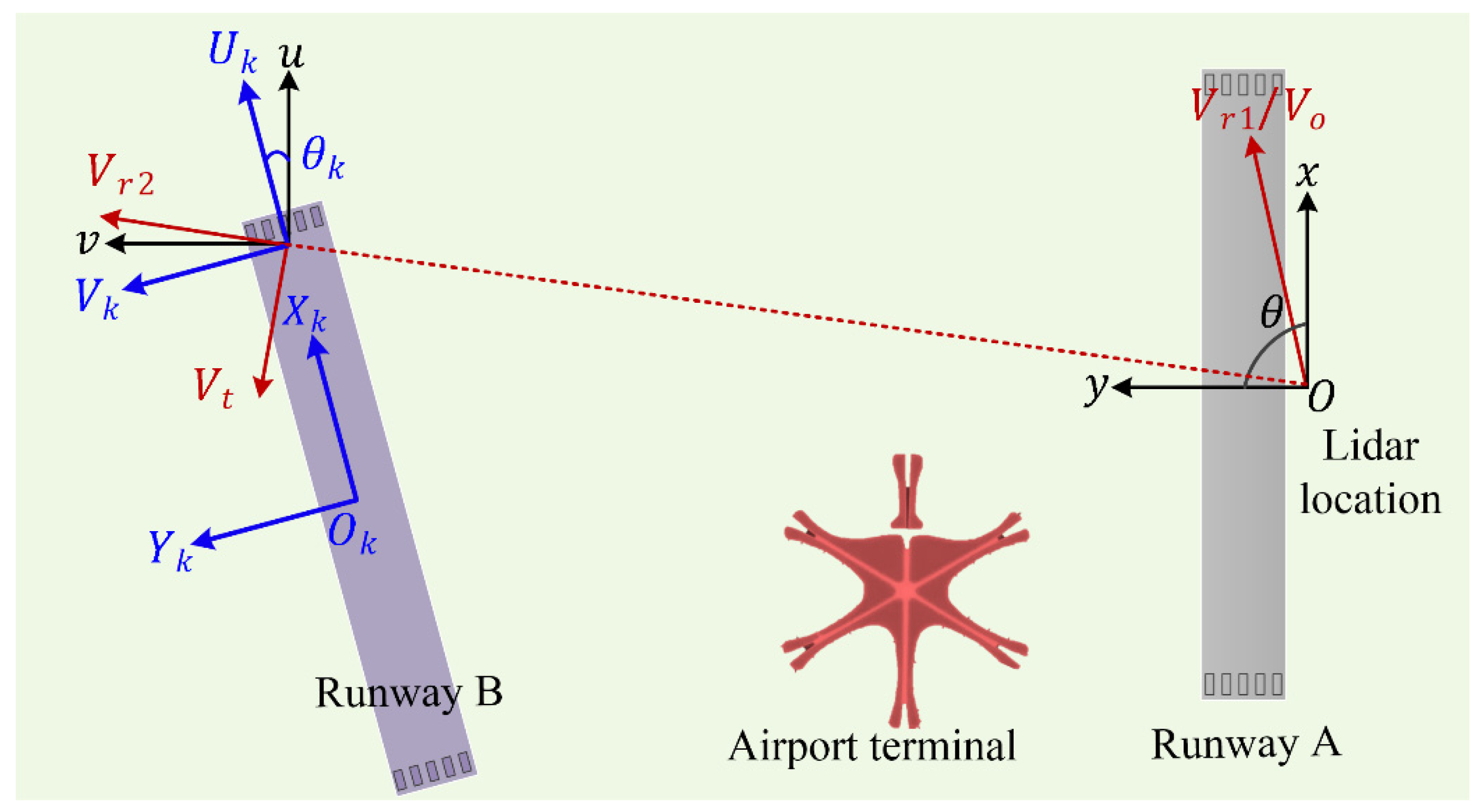
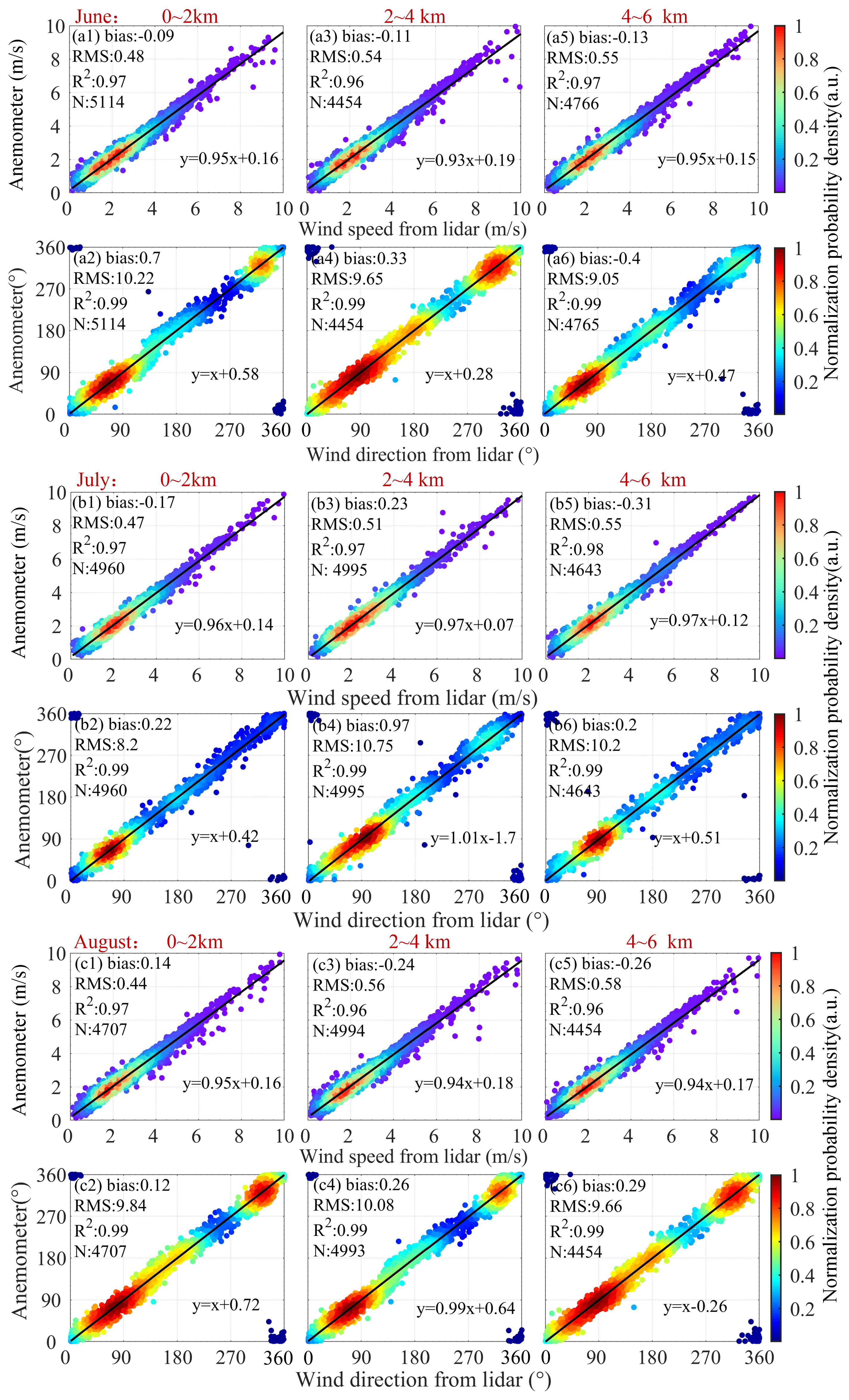
3.1. 2D Wind Field Retrieval and Verification

A comparison with the measurements from the anemometers was carried out at BDIA to determine the capability and estimate the accuracy of 2D wind retrieved from the CDWL. The accuracies of the ultrasonic anemometer (WMT703, Vaisala) for wind speed and wind direction were found to be ±0.1 m/s and ±2°, respectively. An anemometer is located at the middle and at both ends of each runway. The wind data from 9 anemometers located at 17R/35L, 17L/35R, and 01L/19R, were used, which were classified into three groups (0~2 km, 2~4 km, and 4~6 km), according to the distance from the lidar. As raw data management, the carrier-to-noise ratio (CNR) criterion was set to −27 dB, where the radial velocity error of the CDWL does not exceed 0.2 m/s [37]. The angle accuracy reaches 0.01°. Thus, the control precision of tangential displacement is guaranteed, which helps improve the accuracy of retrieval wind. The comparison results for the three consecutive months are shown in Figure 3.
The wind speed is mainly concentrated at 1~3 m/s, while the wind direction varies according to the month. The lidar observations are highly correlated with anemometer observations, with a correlation coefficient of >0.95. The slope of line fitting of the wind speed >0.93, and that of the wind direction >0.99. The bias is marginal between the results of anemometers and CDWL. The magnitude of the RMS for wind speed is less than 0.6 m/s. The magnitude of the RMS for wind direction is less than 11°.

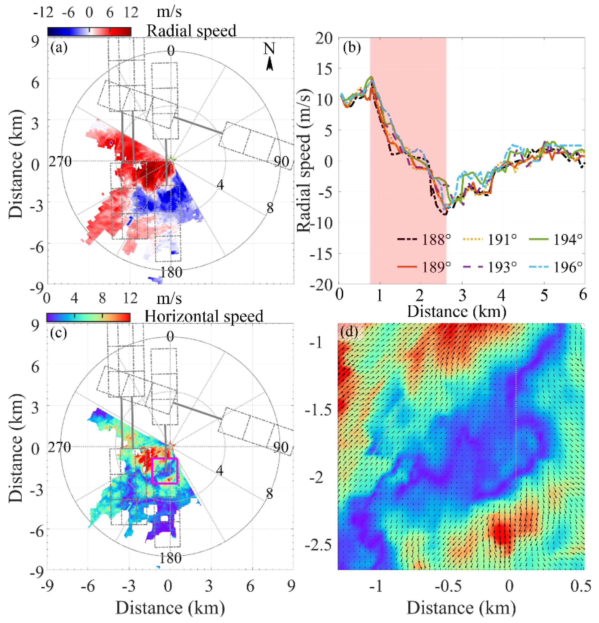
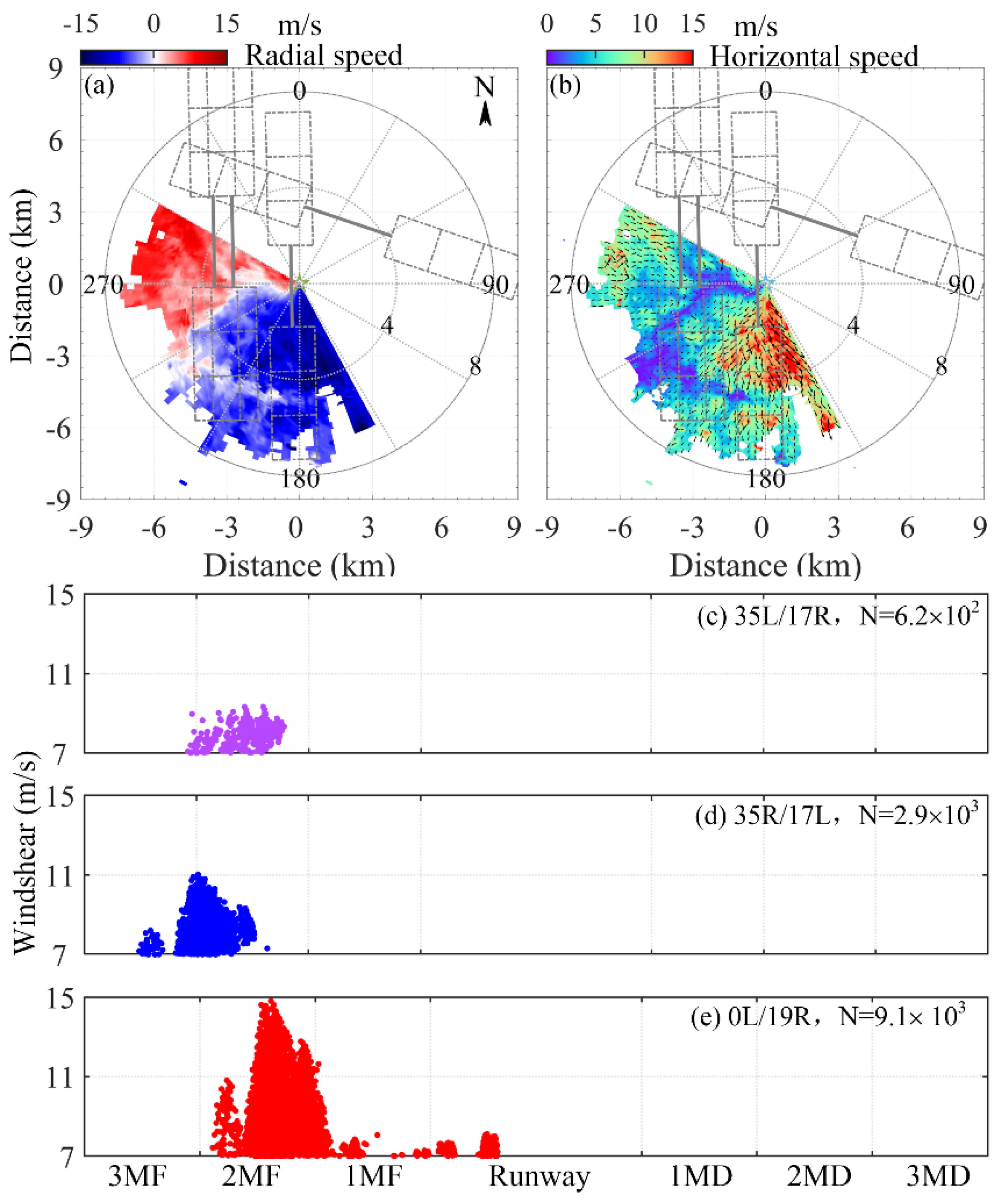
3.2. Microburst Observations

The microburst has a strong divergent structure, which causes a large loss of speed over 15 m/s (30 kt) [1]. The microburst is first introduced in view of dangerous and highly regarded atmospheric disturbances. A typical microburst event was observed on 28 April, 15:53–16:02 (UTC). The radial speed is shown in Figure 4a. Despite the influence of thunderstorm weather, the detection range of the lidar can still reach 5 km. There was a sudden change in radial speed at 2 km southwest of the lidar, where significant divergence velocity pairs were found along the radial direction. Radial speeds at the azimuth angle of 188° to 196° are shown in Figure 4b. The forward speed reaches 14 m/s and changes rapidly to a negative speed of −8 m/s. The difference between the two opposing velocities exceeds 22 m/s within 2 km. The two retrieved wind components are shown in Figure 4c,d. The horizontal wind vector shows an obvious divergence structure. If the aircraft lands from the south glide path, the airspeed will suddenly change from a headwind to a downwind. Such a severe loss of wind speed would seriously threaten aircraft safety.
Figure 5 shows the windshear center distribution on the runway due to the microburst. 3MF, 2MF, and 1MF in the X axis refer to the three monitor subareas in the landing sides, while 3MD, 2MD, and 1MD refer to the monitor subareas in the departure sides. The purple, blue, and red color points represent windshear ramps in 35L/17R, 35R/17L, and 01L/19R, respectively. Windshear ramps larger than 7 m/s are counted, and the number of these ramps reflects the intensity of the wind shear in the monitoring area. A threshold of 500 is adopted for the generation of the windshear message, which is relative to the size of the subarea and spatial resolution. The threshold is chosen through mutual verification with the crew report. The glide paths of the three runways were affected by the microburst, especially for 35R/17L and 01L/19R. These glide paths have many windshear ramps, leading to windshear alert messages. The windshear ramp number of 01L/19R reaches 2.4 × 10⁶, and the maximum windshear exceeds 25 m/s. Three aircrafts encountered windshear when they landed at 35L, as reported by crews.

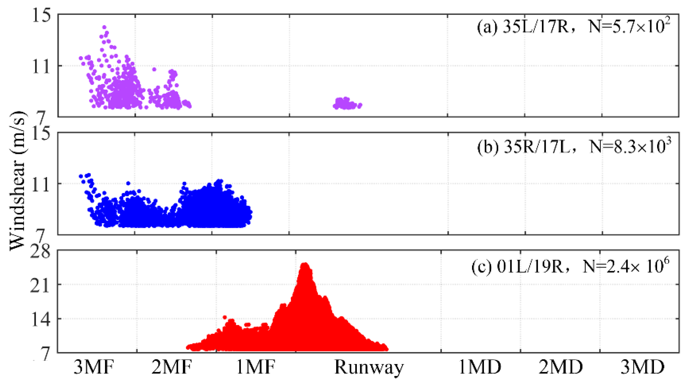
3.3. Genernal Windshear Observations

In addition to the microburst, general windshears occur frequently at airports. These kinds of conventional windshears have weaker intensity compared with microbursts, but their impact on aircraft cannot be ignored.
Two general windshear cases are introduced, which were detected on 6 May, 5:44–5:52 (UTC) and 26 May, 10:23–10:41 (UTC). These two windshears mainly affected the glidepath and runway, respectively. Figure 6 shows the wind field and windshear ramp distribution with an elevation of 3° on 6 May, 05:49:47–05:50:19 UTC, when a windshear event was reported by the crew 3 km away from the landing spot of 35L. There was a distinct low speed zone across the south side of the glide path, as shown in Figure 6a,b. The north wind is dominant, with the maximum wind speed exceeding 15 m/s. Figure 6b–d shows windshear center distribution on the runway, and 2MF of 35L/17R, 3MF and 2MF of 35R/17L, 2MF of 01L/19R were affected by the windshear, which led to windshear alert messages. The windshear center distribution matches the low-speed zone. The windshear alert message at 2MF of 35L/17R was consistent with the windshear reports from the crew.
Figure 7 shows the wind field and windshear ramp distribution with an elevation of 0° on 26 May, 10:33:38–10:34:21 (UTC), when two windshear events were continuously reported by the crew at the runway of 01L at 10:33 and 10:34. The radial speed and horizontal speed are shown in Figure 7a,b. The background wind was mainly westerly with the maximum wind speed exceeding 10 m/s. The runway of 01L/19R was mainly affected by the windshear. A large number of ramps was detected on the runway monitor area, as shown in Figure 7c. It was consistent with the windshear reports from aircrews. The windshear ramp center distributions of 35L/17R and 35R/17L were not drawn, for few windshear ramps were counted.

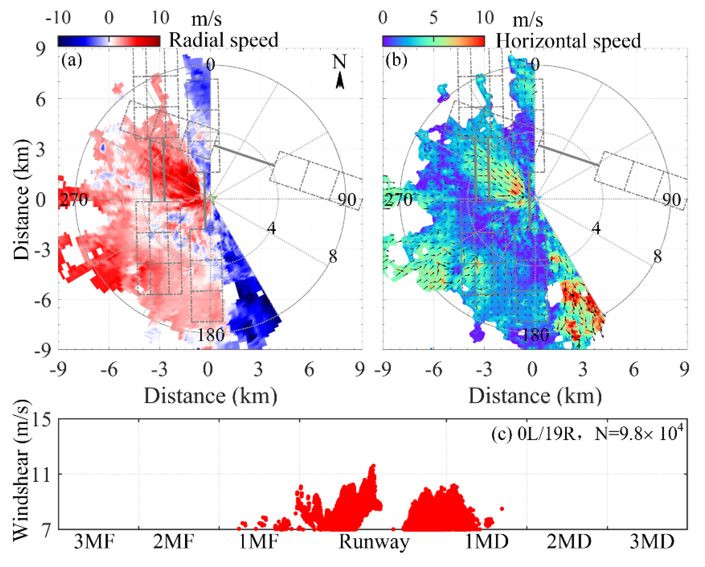
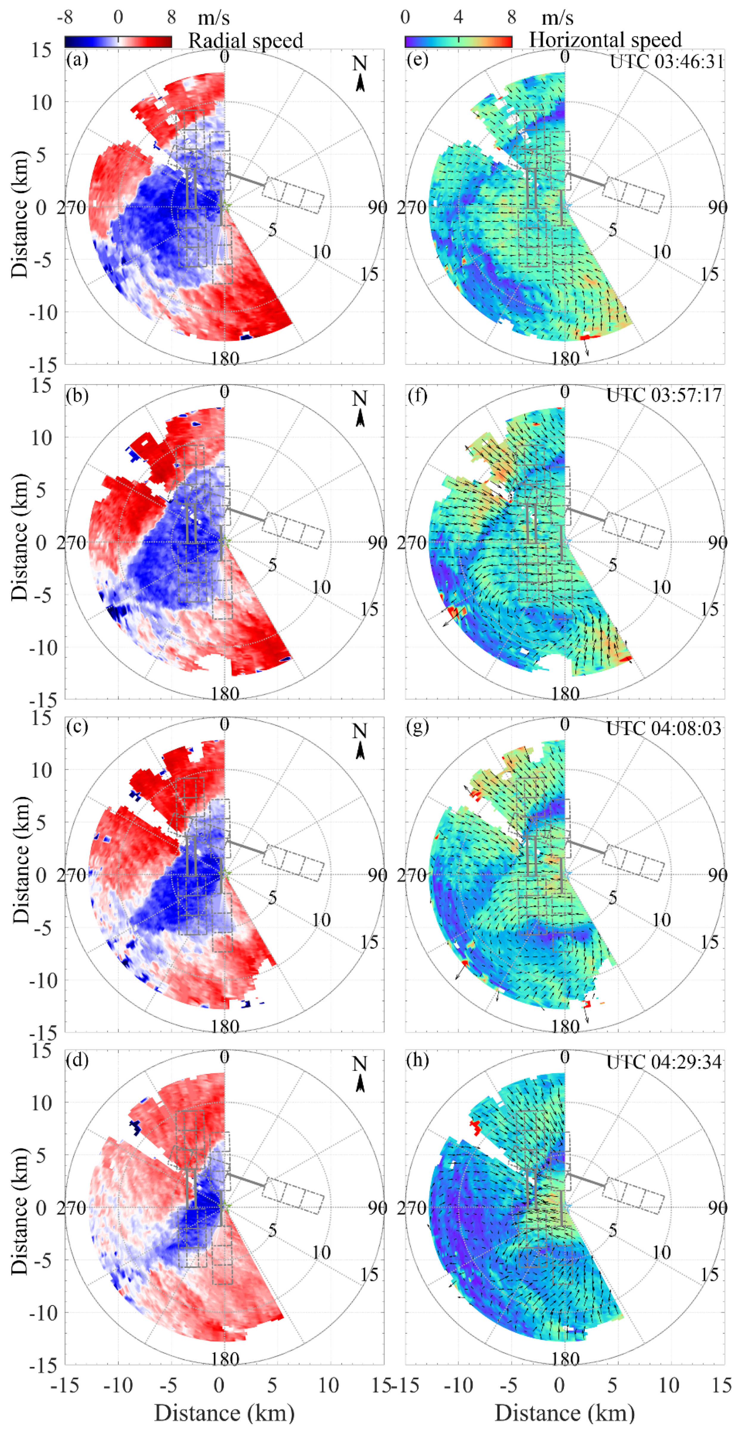
3.4. Gust Front and Vortex Observations

During the experiment, many complex flow phenomena were observed, which pose potential threats to aircraft. Figure 8 shows a continuous process of gust front and vortex structure on 1 July, 3:46–4:29 (UTC).
The maximum detection distance exceeded 12 km. At 3:46, one gust was blowing from the northwest, the other was from the south. The radial velocity was divided into three zones, and each gust front was accompanied by a low velocity zone at the junction of streams, as shown in Figure 8a–d. The two streams of air squeezed each other, resulting in a vortex that spined in reverse time, as shown in Figure 8e–h. The vortex has an influence range of 10 km in the south glide path. As the two air flows come closer, the vortex structure becomes more obvious.
The whole process lasted 43 min. Complex flows such as gust front and vortex can easily lead to a loss of wind speed. Sufficient intensity of front and vortex structures will affect the aircraft takeoff/landing for their wide influence. Through the two-dimensional wind field retrieval, these complex flows can be accurately depicted and identified, which is important to ensure the safety of aircraft.

3.5. Verification by Flight Crew Reports

From 1 April to 6 June 2021, a total of 10 wind shear events were reported by crews, which were collected and provided by BDIA. PoD (Percentage of detection or Hit Rate) and PoTA (Percentage of Time on Alert) are adopted as evaluation indicators for the proposed approach [4,29]. PoD and PoTA are defined as the ratio of the number of hits to total number of pilot reports and the ratio of alert duration to total length of time investigated, respectively.
The relationships between the threshold for the number of windshear ramps and PoD/PoTA are listed in Table 2. A lower threshold ensures a higher PoD value, but corresponding larger PoTA value, resulting in a high false alarm rate. On the contrary, a higher threshold may lead to a missing report. Therefore, an effective and appropriate threshold needs to take into account both PoD and PoTA. When the threshold is set at 500, 100% POD is reached, and PoTA also reaches an acceptably low value of 0.81%, as bolded in Table 2. Since pilot reports are limited for the initial detection, more windshear events need to be accumulated to find an optimized threshold.
Table 3 lists the windshear records from crew reports during the initial detection. These windshear events refer to the fact that pilots encountered significant airspeed loss or gain (usually exceeding 7.7 m/s) along the glide path. The windshear message reported by the crew include the runway number, the distance from the runway, and the height of the aircraft. The windshear alert from lidar includes the runway number, subareas, and windshear value. Most of the windshear events occurred in the landing process from the south. The microburst caused three consecutive windshear events. Windshear alerts from the lidar hit all the events reported by pilots accurately with a threshold of 500, based on the method proposed in this work.

4. Conclusions

A single CDWL-based approach for windshear altering of multiple runways was demonstrated at Beijing Daxing International Airport during the field experiment. With an angle pointing accuracy of 0.01° of the scanning lidar, orthogonal wind components on each runway were retrieved according to continuity airflow, which was consistent with anemometer observations. Due to the high spatial and temporal resolutions of the CDWL, it captured a fine structure of the complex flow, such as the microburst and vortex. The intensity of the microburst is much stronger than that of the general windshear, and the maximum windshear ramps of the microburst exceed 25 m/s. Gusts and vortexes are also noteworthy for their wide range of influence. By traversing and counting all severe shear ramps filtered by the windshear severity factor, the windshear was well evaluated and identified. In the windshear verification experiment, 10 crew reports were accumulated for 66 consecutive days, and the PoTA reached 0.81%, and the PoD reached 100%. This shows that the proposed approach can effectively reduce PoTA. Since pilot reports for verification are limited in the initial detection, more windshear events are needed to find a more optimized threshold by taking into account both PoD and PoTA.
Flights are expected to encounter less windshear in the future with the early alerting of the ground-based lidar. Such verification experiments in the BDIA are helpful for the application of the approach in other airports, which suffer frequent windshear. In the future, we will further extend the capability of new approaches for turbulence and tailwind alerting based on the lidar system.

Author Contributions

Conceptualization, H.X.; Methodology, J.Y. Software, J.Y. and L.S.; Formal Analysis, H.X. and J.Y.; Investigation, J.Y; Resources, J.Y., G.Z., Y.L., M.Z. and J.L.; Data Curation, J.Y.; Writing—Original Draft Preparation, H.X. and J.Y.; Writing—Review and Editing, H.X. and J.Y.; Visualization, J.Y.; Supervision, H.X. All authors have read and agreed to the published version of the manuscript.

Funding

This research received no external funding.

Data Availability Statement

Data underlying the results presented in this paper can be obtained from the authors upon reasonable request.

Acknowledgments

We are grateful to BDIA for providing anemometer data and flight crew reports. We thank Hao Huang, Wei Zhong and Xi Zhang for their contribution to the field experiment.

Conflicts of Interest

The authors declare no conflict of interest.

References

  1. ICAO. Manual on Low-Level Wind Shear; International Civil Aviation Organization: Montreal, QC, Canada, 2005. [Google Scholar]
  2. Yuan, J.; Xia, H.; Wei, T.; Wang, L.; Yue, B.; Wu, Y. Identifying cloud, precipitation, windshear, and turbulence by deep analysis of the power spectrum of coherent Doppler wind lidar. Opt. Express 2020, 28, 37406–37418. [Google Scholar] [CrossRef] [PubMed]
  3. Zhang, H.; Wu, S.; Wang, Q.; Liu, B.; Yin, B.; Zhai, X. Airport low-level wind shear lidar observation at Beijing Capital International Airport. Infrared Phys. Technol. 2019, 96, 113–122. [Google Scholar] [CrossRef] [Green Version]
  4. Wu, T.-C.; Hon, K.-K. Application of spectral decomposition of LIDAR-based headwind profiles in windshear detection at the Hong Kong International Airport. Meteorol. Z. 2018, 27, 33–42. [Google Scholar] [CrossRef]
  5. Li, L.; Shao, A.; Zhang, K.; Ding, N.; Chan, P.-W. Low-Level Wind Shear Characteristics and Lidar-Based Alerting at Lanzhou Zhongchuan International Airport, China. J. Meteorol. Res. 2020, 34, 633–645. [Google Scholar] [CrossRef]
  6. Lin, C.; Zhang, K.; Chen, X.; Liang, S.; Wu, J.; Zhang, W. Overview of Low-Level Wind Shear Characteristics over Chinese Mainland. Atmosphere 2021, 12, 628. [Google Scholar] [CrossRef]
  7. Campbell, M.W.M.D.K.-W.S.D. Wind Shear Detection with Pencil-Beam Radars. Lincoln Lab. J. 1989, 2, 483–510. [Google Scholar]
  8. Goff, R.C. The Low-Level Wind Shear Alert System (LLWSAS); National Aviation Facilities Experimental Center: Atlantic City, NJ, USA, 1980. [Google Scholar]
  9. Zhang, Y.; Guo, J.; Yang, Y.; Wang, Y.; Yim, S. Vertical Wind Shear Modulates Particulate Matter Pollutions: A Perspective from Radar Wind Profiler Observations in Beijing, China. Remote Sens. 2020, 12, 546. [Google Scholar] [CrossRef] [Green Version]
  10. Yim, S.H.L. Development of a 3D Real-Time Atmospheric Monitoring System (3DREAMS) Using Doppler LiDARs and Applications for Long-Term Analysis and Hot-and-Polluted Episodes. Remote Sens. 2020, 12, 1036. [Google Scholar] [CrossRef] [Green Version]
  11. Hirsikko, A.; O’Connor, E.J.; Komppula, M.; Korhonen, K.; Pfüller, A.; Giannakaki, E.; Wood, C.R.; Bauer-Pfundstein, M.; Poikonen, A.; Karppinen, T.; et al. Observing wind, aerosol particles, cloud and precipitation: Finland’s new ground-based remote-sensing network. Atmos. Meas. Tech. 2014, 7, 1351–1375. [Google Scholar] [CrossRef] [Green Version]
  12. Wang, L.; Qiang, W.; Xia, H.; Wei, T.; Yuan, J.; Jiang, P. Robust Solution for Boundary Layer Height Detections with Coherent Doppler Wind Lidar. Adv. Atmos. Sci. 2021, 38, 1920–1928. [Google Scholar] [CrossRef]
  13. Jia, M.; Yuan, J.; Wang, C.; Xia, H.; Wu, Y.; Zhao, L.; Wei, T.; Wu, J.; Wang, L.; Gu, S.Y.; et al. Long-lived high-frequency gravity waves in the atmospheric boundary layer: Observations and simulations. Atmos. Chem. Phys. 2019, 19, 15431–15446. [Google Scholar] [CrossRef] [Green Version]
  14. Chan, P.W. LIDAR-based turbulence intensity calculation using glide-path scans of the Doppler LIght Detection and Ranging (LIDAR) systems at the Hong Kong International Airport and comparison with flight data and a turbulence alerting system. Meteorol. Z. 2010, 19, 549–563. [Google Scholar] [CrossRef]
  15. Banakh, V.; Smalikho, I. Lidar Studies of Wind Turbulence in the Stable Atmospheric Boundary Layer. Remote Sens. 2018, 10, 1219. [Google Scholar] [CrossRef] [Green Version]
  16. O’Connor, A.; Kearney, D. Low Level Turbulence Detection for Airports. Int. J. Aviat. Aeronaut. Aerosp. 2019, 6. [Google Scholar] [CrossRef] [Green Version]
  17. Tuononen, M.; O’Connor, E.J.; Sinclair, V.A.; Vakkari, V. Low-Level Jets over Utö, Finland, Based on Doppler Lidar Observations. J. Appl. Meteorol. Clim. 2017, 56, 2577–2594. [Google Scholar] [CrossRef]
  18. Pantillon, F.; Wieser, A.; Adler, B.; Corsmeier, U.; Knippertz, P. Overview and first results of the Wind and Storms Experiment (WASTEX): A field campaign to observe the formation of gusts using a Doppler lidar. Adv. Sci. Res. 2018, 15, 91–97. [Google Scholar] [CrossRef]
  19. Smalikho, I.N.; Banakh, V.A.; Holzapfel, F.; Rahm, S. Method of radial velocities for the estimation of aircraft wake vortex parameters from data measured by coherent Doppler lidar. Opt. Express 2015, 23, A1194–A1207. [Google Scholar] [CrossRef] [Green Version]
  20. Nechaj, P.; Gaal, L.; Bartok, J.; Vorobyeva, O.; Gera, M.; Kelemen, M.; Polishchuk, V. Monitoring of Low-Level Wind Shear by Ground-based 3D Lidar for Increased Flight Safety, Protection of Human Lives and Health. Int J. Environ. Res. Public Health 2019, 16, 4584. [Google Scholar] [CrossRef] [PubMed] [Green Version]
  21. Liu, Z.; Barlow, J.F.; Chan, P.-W.; Fung, J.C.H.; Li, Y.; Ren, C.; Mak, H.W.L.; Ng, E. A Review of Progress and Applications of Pulsed Doppler Wind LiDARs. Remote Sens. 2019, 11, 2522. [Google Scholar] [CrossRef] [Green Version]
  22. Thobois, L.; Cariou, J.P.; Gultepe, I. Review of Lidar-Based Applications for Aviation Weather. Pure Appl. Geophys. 2018, 176, 1959–1976. [Google Scholar] [CrossRef]
  23. Huang, J.; Ng, M.K.P.; Chan, P.W. Wind Shear Prediction from Light Detection and Ranging Data Using Machine Learning Methods. Atmosphere 2021, 12, 644. [Google Scholar] [CrossRef]
  24. Hon, K.K.; Chan, P.W.; Chiu, Y.Y.; Tang, W. Application of Short-Range LIDAR in Early Alerting for Low-Level Windshear and Turbulence at Hong Kong International Airport. Adv. Meteorol. 2014, 2014. [Google Scholar] [CrossRef]
  25. Chan, P.W. Severe wind shear at Hong Kong International Airport: Climatology and case studies. Meteorol. Appl. 2017, 24, 397–403. [Google Scholar] [CrossRef] [Green Version]
  26. Chan, P.W.; Lai, K.K.; Li, Q.S. High-resolution (40 m) simulation of a severe case of low-level windshear at the Hong Kong International Airport—Comparison with observations and skills in windshear alerting. Meteorol. Appl. 2021, 28. [Google Scholar] [CrossRef]
  27. Lee, Y.F.; Chan, P.W. Application of Short-Range Lidar in Wind Shear Alerting. J. Atmos. Ocean. Tech. 2012, 29, 207–220. [Google Scholar] [CrossRef]
  28. Chan, P.W.; Shun, C.M. Applications of an Infrared Doppler Lidar in Detection of Wind Shear. J. Atmos. Ocean. Tech. 2008, 25, 637–655. [Google Scholar] [CrossRef]
  29. Hon, K.K.; Chan, P.W. Improving Lidar Windshear Detection Efficiency by Removal of “Gentle Ramps”. Atmosphere 2021, 12, 1539. [Google Scholar] [CrossRef]
  30. Yoshino, K. Low-Level Wind Shear Induced by Horizontal Roll Vortices at Narita International Airport, Japan. J. Meteorol. Soc. Jpn. 2019, 97, 403–421. [Google Scholar] [CrossRef] [Green Version]
  31. van Dooren, M.F.; Campagnolo, F.; Sjöholm, M.; Angelou, N.; Mikkelsen, T.; Kühn, M. Demonstration and uncertainty analysis of synchronised scanning lidar measurements of 2-D velocity fields in a boundary-layer wind tunnel. Wind Energy Sci. 2017, 2, 329–341. [Google Scholar] [CrossRef] [Green Version]
  32. Chan, P.W.; Shao, A.M. Depiction of complex airflow near Hong Kong International Airport using a Doppler LIDAR with a two-dimensional wind retrieval technique. Meteorol. Z. 2007, 16, 491–504. [Google Scholar] [CrossRef]
  33. Qiu, C.J.; Shao, A.M.; Liu, S.; Xu, Q. A two-step variational method for three-dimensional wind retrieval from single Doppler radar. Meteorol. Atmos. Phys. 2005, 91, 1–8. [Google Scholar] [CrossRef]
  34. Chan, P.W.; Hon, K.K.; Shin, D.K. Combined use of headwind ramps and gradients based on LIDAR data in the alerting of low-level windshear/turbulence. Meteorol. Z. 2011, 20, 661–670. [Google Scholar] [CrossRef]
  35. Woodfield, A.; Woods, J. Wind Shear from Head Wind Measurements on British Airways B747-236 Aircraft; Royal Aircraft Establishment Bedford: Bedford, UK, 1981. [Google Scholar]
  36. Woodfield, A.A.; Woods, J.F. Worldwide Experience of Wind Shear During 1981–1982; Royal Aircraft Establishment Bedford: Bedford, UK, 1983. [Google Scholar]
  37. Wang, C.; Xia, H.; Shangguan, M.; Wu, Y.; Wang, L.; Zhao, L.; Qiu, J.; Zhang, R. 1.5 μm polarization coherent lidar incorporating time-division multiplexing. Opt. Express 2017, 25, 20663–20674. [Google Scholar] [CrossRef] [PubMed] [Green Version]
Figure 1. Diagrams of coordinates and velocities.
Remotesensing 14 01626 g001
Figure 2. (a) The location of the CDWL at BDIA, (b) Photograph of the CDWL.
Remotesensing 14 01626 g002
Figure 3. Comparison results of wind speed and direction measured by anemometers and retrieved from the CDWL. (a1a6), (b1b6) and (c1c6) shows the comparison result of June, July, and August, respectively. The detail linear fitting results are also given in the figure. The color of each points represents the normalization probability density using the kernel density estimation. Positions of anemometers are marked in the head of each group of diagrams in red font.
Remotesensing 14 01626 g003
Figure 4. Microburst results detected by the CDWL on 28 April, 15:54:12–15:54:42 (UTC). (a,b) radial speed, (c) horizontal speed. The pink rectangle means the area most affected by microburst. The detail structure of horizontal speed in pink rectangle in (c) is shown in (d). The sign of radial speed is defined as positive when the movement is toward the lidar, and vice versa.
Remotesensing 14 01626 g004
Figure 5. Windshear center distribution on the runway due to the microburst, on 28 April, 15:54:12–15:54:42 (UTC). (a) 35L/17R, (b) 35R/17L, (c) 01L/19R. N is the number of windshear ramps that exceed 7 m/s. 3MF, 2MF, and 1MF in the X axis mean the three monitor subareas in the landing sides, while 3MD, 2MD, and 1MD mean the monitor subareas in the departure sides.
Remotesensing 14 01626 g005
Figure 6. The windshear event detected by the CDWL on May 6, 05:49:47–05:50:19 (UTC). (a) Radial speed, (b) horizontal speed and wind vector, (ce) windshear ramps center distribution of 35L/17R, 35R/17L, 01L/19R. N is the number of windshear ramps that exceed 7 m/s.
Remotesensing 14 01626 g006
Figure 7. The windshear event detected by the CDWL on May 26, 10:33:38–10:34:21 (UTC). (a) Radial speed, (b) horizontal speed and wind vector, (c) windshear ramps center distribution. N is the number of windshear ramps that exceed 7 m/s.
Remotesensing 14 01626 g007
Figure 8. The windshear event detected by the CDWL on July 1. (UTC). (ad) Radial speed, (eh) Horizontal speed. (a,e) 3:46:31–3:47:12, (b,f) 3:57:17–3:57:58, (c,g) 4:08:03–4:08:45, (d,h) 4:29:34–4:30:17.
Remotesensing 14 01626 g008
Table 1. Key Parameters of the CDWL.
ParameterValue
Wavelength1.5 μm
Pulse Energy300 μJ
Diameter of telescope80 mm
Repetition frequency10 kHz
Diameter of telescope80 mm
Temporal resolution0.2–1 s
Spatial resolution30 m
Angle accuracy0.01°
Maximum range13 km
Azimuth scanning range0–360°
Zenith scanning range0–90°
Table 2. The relationship between threshold and PoD/ PoTA.
Windshear ThresholdPOD (%)PoTA (%)
5010012.69
1001007.77
2001003.51
3001001.77
4001001.31
5001000.81
600900.69
700800.55
800800.34
900700.22
1000700.16
Table 3. Windshear event reports from crew.
Time (UTC)Runway, Position, Height (Crew)Windshear Alert from Lidar
28 April, 15:5535L, 3 km, 200 m35L, 1.9 km–3.7 km (2MF), −9.9 m/s
28 April, 15:5835L, Runway35L, RWY, −8.2 m/s
28 April, 16:0135L, Runway35L, RWY, −8.7 m/s
6 May, 5:5035L, 3 km, 150 m35L, 1.9 km–3.7 km (2MF), −8.2 m/s
6 May, 8:3701L, 3 km, 150 m01L, 1.9 km–3.7 km (2MF), −8.6 m/s
6 May, 11:0535L, Runway35L, RWY, −8.3 m/s
26 May, 10:3301L, Runway01L, RWY, −7.7 m/s
26 May, 10:3401L, Runway01L, RWY, −8.9 m/s
26 May, 10:4001L, 5 km,250 m01L, 3.7 km–5.6 km (3MF), −9.6 m/s
5 June, 11:5401L, 4 km,200 m01L, 3.7 km–5.6 km (3MF), −15.9 m/s
Publisher’s Note: MDPI stays neutral with regard to jurisdictional claims in published maps and institutional affiliations.

