
Assessment of RTK Quadcopter and Structure-from-Motion Photogrammetry for Fine-Scale Monitoring of Coastal Topographic Complexity


1
UMR 6538 Geo-Ocean, University Brest-CNRS-Ifremer, Institut Universitaire Européen de la Mer, Rue Dumont d’Urville, 29280 Plouzané, France
2
UAR 3113 Institut Universitaire Européen de la Mer (IUEM), University Brest-CNRS, Rue Dumont d’Urville, 29280 Plouzané, France
3
UMR 6554 Littoral, Environnement, Géomatique, Télédétection, University Brest-CNRS, Institut Universitaire Européen de la Mer, Rue Dumont d’Urville, 29280 Plouzané, France
*
Author to whom correspondence should be addressed.
Remote Sens. 2022, 14(7), 1679; https://doi.org/10.3390/rs14071679
Submission received: 7 March 2022
/
Revised: 24 March 2022
/
Accepted: 29 March 2022
/
Published: 31 March 2022
(This article belongs to the Special Issue Remote Sensing for Coastal and Aquatic Ecosystems’ Monitoring and Biodiversity Management)
Abstract
:Advances in image-based remote sensing using unmanned aerial vehicles (UAV) and structure-from-motion (SfM) photogrammetry continue to improve our ability to monitor complex landforms over representative spatial and temporal scales. As with other water-worked environments, coastal sediments respond to shaping processes through the formation of multi-scale topographic roughness. Although this topographic complexity can be an important marker of hydrodynamic forces and sediment transport, it is seldom characterized in typical beach surveys due to environmental and technical constraints. In this study, we explore the feasibility of using SfM photogrammetry augmented with an RTK quadcopter for monitoring the coastal topographic complexity at the beach-scale in a macrotidal environment. The method had to respond to resolution and time constraints for a realistic representation of the topo-morphological features from submeter dimensions and survey completion in two hours around low tide to fully cover the intertidal zone. Different tests were performed at two coastal field sites with varied dimensions and morphologies to assess the photogrammetric performance and eventual means for optimization. Our results show that, with precise image positioning, the addition of a single ground control point (GCP) enabled a global precision (RMSE) equivalent to that of traditional GCP-based photogrammetry using numerous and well-distributed GCPs. The optimal model quality that minimized vertical bias and random errors was achieved from 5 GCPs, with a two-fold reduction in RMSE. The image resolution for tie point detection was found to be an important control on the measurement quality, with the best results obtained using images at their original scale. Using these findings enabled designing an efficient and effective workflow for monitoring coastal topographic complexity at a large scale.
1. Introduction
The coast is a very dynamic and varied environment, constantly changing in response to complex interrelations between landforms and processes operating across a wide range of spatial and temporal scales. Understanding shoreline dynamics, for integration into process-based modelling, for example, and being able to predict future evolutions in the context of relative sea-level rise, requires an accurate characterization of the geomorphic processes acting at the sediment–water interface [1,2,3,4,5]. Sediment reworking on the beach and nearshore due to waves and currents traduces by the formation of topographic complexity (herewith generally called roughness), such as sedimentary bedforms. These topo-morphological features are the imprint of the processes that shaped them, and, as such, measuring bedforms can provide meaningful information on hydrodynamic forces [6,7,8,9,10]. Besides, bedforms are roughness elements that modify the flow and dissipate energy [11,12]. They are, thus, interesting markers of the sediment bed propensity towards resistance to entrainment and dynamic equilibrium.
Different types of bedforms generally coexist in the coastal environment (e.g., Refs. [13,14,15]), whose dimensions and shapes depend on sediment availability, sediment type (e.g., size distribution and shape) and driving mechanisms (e.g., waves, currents, wind). Examples of small-scale bedforms are wave and current sand ripples, or gravel-bed clusters, with dimensions or length scales generally not exceeding a few tens of centimeters. Larger-scale bedforms include varied bar and trough morphologies (e.g., ridge and runnels) in the surf and swash zones [16], other rhythmic patterns most often found on the upper beach, such as beach cusps [17,18], as well as aeolian sand dunes. In between those, there are a wide range of topographic variations that take part in the continuum of roughness scales and contribute to the overall structural complexity of the seabed, backshore and dune system.
1.1. High-Resolution Topographic Surveying and Photogrammetric Remote Sensing of Coastal Morphology
In tidal environments, daily fluctuations in the water level mean that the water-worked seabed can be measured using topographic surveying, with the maximum coverage typically achieved during the lowest low tides. Previous work largely relied on RTK-GNSS, with a rover eventually mounted on a mobile platform, such as a quad, for monitoring the evolution of barred beaches and other coastal landforms [12,19]. The DEMs generated have resolutions ranging from a few meters cross-shore to tens of meters alongshore, in link with the topographic complexity and bedform orientation, while survey coverage can reach up to several kilometers alongshore, allowing to account for the rhythmic nature of the coastal morphology (e.g., rip-channel systems, cusps and megacusps). Common to point-based surveying techniques, enhancing the spatial resolution is generally counter-balanced by increased acquisition time or reduced spatial coverage [20,21,22], which means that using RTK-GNSS for the fine-scale monitoring of coastal topography remains problematic.
In contrast, remote sensing techniques, such as UAV photogrammetry, have greatly improved, rendering very-high-resolution (e.g., submeter) topographic surveying at a large scale (e.g., beach scale) feasible. Using off-the-shelf drones and cameras, ground sampling distances (GSD) as small as a few centimeters can be achieved during typical beach surveys [23,24,25]. Photogrammetric processing relies on the SfM method, which is based on the scale-invariant feature transform (SIFT) algorithm [26] for matching corresponding points in images, and uses external information, mostly taking the form of GCPs measured independently, for scaling and optimizing the photogrammetric model. Yet, previous work showed that the resulting DEM quality (e.g., horizontal and vertical precisions) is largely variable (e.g., Refs. [23,27,28]) and depends on a wide range of parameters, among which survey design (e.g., flying height, image overlap, camera orientation, GCP number and distribution) and processing strategies (e.g., direct georeferencing, camera calibration and point-matching methods) play a critical role.
Photogrammetry has been used previously in different domains of research to measure sedimentary bedforms of various dimensions, including particle clusters [29,30], bed undulations, such as sand [31,32,33] and gravel bars [34,35,36], and sand dunes [37,38,39,40,41,42], with measurements of small-scale bedforms generally performed in the laboratory. Hence, it is not yet known if fine-scale water-worked topographies can be efficiently and effectively measured using UAV photogrammetry in the field, such that there is currently a paucity of data for assessing coastal topographic roughness and shaping processes.
1.2. Photogrammetric Workflow Optimisation
A common limitation to achieving efficient surveys mentioned in previous work, and finding important echo in time-constrained (e.g., tidal) environments, is the need for a dense and well-measured network of GCPs for the accurate scaling and georeferencing of photogrammetric results (e.g., Ref. [43]). In the absence of other external controls, this requirement is particularly important, shown by observations of decreasing DEM quality with distance increases from the nearest GCP [44,45,46]. Relief can be procured through the installation of fixed (i.e., permanent) targets, although it is generally only partial and, in application to the coast, implies that fixed targets are limited to dry zones [37].
The uptake of high-precision RTK-GNSS technology for drone navigation can further improve survey efficiency. With RTK drones, image geolocations serve as airborne controls, which, despite a generally lower precision compared to GCPs and a repartition outside the measurement volume, can compensate for these caveats due to the comparatively very-large number of controls provided [47]. Previous research showed that results of a similar quality or even better can be achieved using a reduced number of GCPs when the camera positions are used as external controls [48]. Using the camera information as the only external control during photogrammetric processing forms the basis behind direct georeferencing (DG) approaches (e.g., Refs. [49,50,51]). The DG of photogrammetry is particularly advantageous when access to the field site and the measurement of GCPs are problematic. However, previous studies showed that DG generally comes at the cost of reduced measurement quality (e.g., lower accuracy and precision).
The commercialization of RTK drones at competitive prices (e.g., the Phantom 4 RTK quadcopter) has reinstated large interest in determining the capability of DG approaches across different settings, including building facades, urban and rural landscapes as well as river and coastal environments. Previous studies investigated the differences between drone positioning corrections provided either in real time (RTK) from a nearby base station managed by the field operators or through RTK networks, or post-processed (PPK) using observations at known base stations [52,53]. They also assessed the effect of the image viewing angle (nadir vs. oblique [54]), as well as changes in measurement quality with and without the provision of GCPs (e.g., Refs. [52,53,54,55,56]).
These studies concluded that, in the absence of GCPs, systematic error mainly through vertical bias can impact the measurement quality, which was related to the imprecise calibration of internal orientation parameters (IOP). Yet, contrasting results were obtained when it comes to the number of GCPs to introduce to correct this effect. Some studies reported that one GCP was enough, although the GCP position may be important, while other studies recommended using at least three GCPs. With the exception of the effort to survey 109 points with a theodolite on a building’s facades by Taddia et al. [52], error evaluation is generally limited to a few check points (ChkPts), whose number and repartition may not be adequate for reliable error characterization. This, in turn, limits the generalization of the findings such that the measurement capabilities of RTK-assisted UAV photogrammetry over large and GCP-poor coastal tracts are not fully understood.
1.3. Paper Overview
In this study, we explored the feasibility of using an RTK quadcopter (Phantom 4 RTK) and SfM photogrammetry for fine-scale (e.g., submeter) monitoring of water-worked coastal topography. We carried out a variety of tests of interest for the application because of their influences on data collection time and measurement quality (e.g., resolution and precision). More specifically, we were interested in enhancing the survey efficiency to surpass tide-related constraints while ensuring the results’ effectiveness through rigorous error characterization at two macrotidal coastal field sites with contrasting survey areas and morphologies. The DEM error evaluation at localized check points (ChkPts) was supplemented where possible by full DEM comparisons and the collection of over 2000 survey points with RTK-GNSS, whilst the availability of repeat surveys and invariant features enabled the assessment of the complete workflow replicability.
Our results show that at least five GCPs, in addition to camera information, were necessary to achieve the optimal model quality that minimized vertical bias and random errors. Under this configuration, the standard deviation of error representing measurement precision (~1 GSD) was approximately two times better than that when camera information was unused. First, the geomorphic analyses are presented, highlighting the potential of the method for submeter bedform characterization over entire beach systems.
2. Materials and Methods
2.1. Field Sites
The two coastal field sites presented in this study are located in Brittany in northwest France (Figure 1a,b). The field site at La Palue and Lostmarc’h beaches, hereafter generally referred to as “La Palue” for concision, is situated at the western end of Crozon Peninsula. Facing due west, La Palue and Lostmarc’h are adjacent beaches totaling ~2.5 km alongshore separated by a rocky promontory (Kerdra point) at high tide, backed by granitic cliffs (20–50 m high) at each end point and a mostly consolidated and vegetated dune elsewhere. It is a macrotidal environment with mean neap and spring tidal ranges of 2.25 and 5.60 m [57], respectively. Waves originate from Atlantic depressions generating SW through NW swells, but also shorter period seas from locally generated wind [58]. Based on samples collected on the intertidal beach and processed using traditional size-sieving, sediment belongs to fine to medium sand with a D50 (the median sediment size for which 50% of the sediment distribution is finer) of ~0.25 mm and a sorting coefficient () of 1.35 (i.e., well-sorted). The upper beach abutting the dune is composed of cobbles, especially on the northern parts (Figure 2b). The morphodynamics are akin to intermediate beaches according to the Masselink and Short classification [59], covering a range of beach states depending on ongoing hydrodynamic conditions. Generally, a flatter profile is observed over winter, contrasting with marked bar and rip channel morphologies developing across calmer months. During spring tides, the intertidal beach is approximately 300–400 m wide (Figure 1c). Large patches of ripples and megaripples can often be observed. Bedrock may locally appear near the low-tide line, depending on sand levels. Outside a few of channelized access points and small blockhouses remnant of World War 2, human encroachments are limited. Man-made features, at the condition they are relatively flat, were useful for preparing fixed ground targets for photogrammetry. Depending on survey date, up to six red-painted crosses approximately 40 cm in size were used (Table 1).
The second field site corresponds to the proximal section of the Sillon de Talbert gravel spit. This 3.5-km-long swash-aligned barrier is located north of Brittany. The sediment volume is estimated at 1.23 × 10⁶ m³ [60]. According to the barrier morphology and sedimentology, the gravel accumulation can be classed as a “composite gravel beach” [61,62]. The beach face shows a break slope point at the mean water level, which delimitates the gravel barrier from an otherwise flat rocky platform (slope = 0.01%) covered by thin and patchy periglacial deposits and/or recent sandy sheets. The upper part of the beach face is characterized by steeper slopes of between 5% and 15%. Back-barrier areas include a large sand-flat and salt-marshes. The site is located in a macrotidal to megatidal setting (maximum tidal range of 10.95 m) [57]. Dominant swell comes from the WNW, which means that waves break with a slight angle according to the shoreline orientation, generating a longshore drift oriented to the NE. Until the end of the 17th century, the barrier was connected to the islets of the Olone archipelago located to the NE. The disconnection of the barrier occurred in the early 18th century [63]. In the 1970s and 1980s, several coastal defenses were installed to prevent the retreat of the barrier, especially in the proximal section where a groin was installed. Annual topographic surveys realized with RTK-GNSS since 2002 revealed a strong erosion of the beach face downdrift of the groin [64]. The loss of sediment was estimated to ca. 11,000 m3 between 2002 and 2017, which caused significant barrier lowering and narrowing locally. These morphological changes led to the opening of a breach at the beginning of March 2018, which has experienced a rapid enlargement (35 vs. 15 m) and deepening (3.4 vs. 1.25 m) over the following months [65]. For monitoring breach evolution, we have put in place trimestral UAV photogrammetry surveys.
2.2. Field Operation and Data Collection
Five surveys altogether covering a seven-month period are considered in this study: one at Sillon de Talbert and four at La Palue (Table 1). For the latter, only the first survey (17 September 2020) is described and analyzed in detail, the other three (repeat) surveys being used for assessing measurements’ replicability (cf. Section 2.6).
Data collection starts with centimetric-accuracy RTK-GNSS (Topcon Hyper V) measurements of geodetic marks (cast metal disks installed on stable ground) and photogrammetric targets (red plastic plates 30 cm in diameter fixed to the ground using tent poles) for data georeferencing and validation (cf. Figure 2). Between 20 and 30 photogrammetric targets, including fixed targets, were deployed to be used either as GCPs or ChkPts (cf. Table 1 and Table 2). Measurements are carried out in rapid-static mode (10 s average) using GNSS rovers mounted on a 2-m pole equipped with a bubble level. To provide RTK corrections, a GNSS base station was materialized at both sites using a geodetic mark. Fixed coordinates were obtained using long-static averaging with a tripod (~240 min), over several periods of time, and postprocessed in comparison with nearby IGN (Institut Géographique National) GNSS stations. Repeated measurements of other geodetic marks provide insights on georeferencing quality. For example, using between three and seven survey marks, the standard error (SE) was estimated to be 0.004 m horizontally and 0.002 m vertically on average at La Palue across four consecutive surveys. Geographic coordinates are referenced to the French legal systems for this region, i.e., RGF93-Lambert 93 for planimetry and NGF-IGN69 for altimetry. Elevation zero (m NGF) corresponds to approximately 0.5 m below mean sea level (MSL).
Aerial image acquisition for photogrammetry was carried out using DJI’s Phantom 4 RTK quadcopter (P4 RTK) and D-RTK2 mobile station. The latter is used for drone RTK positioning. According to the manufacturer, this system allows image georeferencing precisions of 1 cm + 1 ppm (parts per million, i.e., 1 mm per 1000 m) and 1.5 cm + 1 ppm along the horizontal and vertical directions, respectively, traducing to absolute accuracies of around 0.05 m at a flying height of 100 m. During surveys, the D-RTK2 is positioned atop a geodetic mark with known coordinates (explanations above). The P4 RTK is equipped with a 20-megapixel (2.41 × 2.41-pixel size) complementary metal-oxide-semiconductor (CMOS) camera (FC6310R) with a mechanical global shutter and an 8.8 mm focal length. Besides precise positioning, the drone attitude (pitch, roll and yaw angles) is recorded automatically for each image using an onboard inertial measurement unit (IMU). For collecting images, we used a single photogrammetric block arrangement with a front and side overlap of 80% and 70%, respectively (Table 1, Figure 2) and a forward-looking camera angle of 6° off-nadir. The flying height, and, thus, the GSD, was adjusted depending on the field site in order to complete surveys within two hours around low tide. The flying height (relative to take-off elevation) was maintained at approximately 58 m and 106 m for the Sillon de Talbert and La Palue field sites, traducing to a GSD of 0.014 m and 0.026 m, respectively. To satisfy local drone regulations active at the sites, five flights, from five different take-off and landing spots, were necessary at La Palue, whereas two flights were enough to cover the breach at Sillon de Talbert. Flight pattern was designed to include an overlap between each image block (cf. Figure 2) while ensuring that flight duration remained below the 20-min mark. Before performing the flights, camera settings were tentatively adjusted to the environmental conditions.
Additional topographic measurements were carried out at La Palue using RTK-GNSS (Figure 2a) to serve as vertical ground truths for the evaluation of photogrammetry. To make for an efficient survey covering as much of the beach length as possible, a GNSS rover was securely mounted onto a bike, using a pannier rack above the rear wheel. The rover was mounted with the antenna pointing downwards (vertically) and aligned with the rear wheel axis. The approximate height of the antenna center above the ground was measured, using a tape ruler, to be ~0.60 m. Determination of the exact height was completed using a geodetic mark, with the bike positioned atop and loaded to replicate survey conditions. The height of the antenna center was used to reference the data into the same coordinate system as other surveys presented above. Point sampling along the beach using the “bike GNSS” was carried out in dynamic mode at 1 Hz. The survey was limited to the intertidal zone close to the low-tide water line with packed sand and where photogrammetric quality was expected to be lower due to the difficulty of deploying GCPs and more generally because of the presence of water, the latter making for more challenging tie point detection. Surveying was done by riding the bike alongshore (cf. Figure 2a) to limit as much as possible introducing a pitch angle between the GNSS antenna and the vertical. Roll minimization was made possible by a bubble level mounted onto the bike handlebar. Strategies to account for pitch and roll-related errors on point coordinates were implemented and will be presented in Section 2.5.
2.3. Photogrammetric Data Processing: Standard Workflow
Drone images were processed using the SfM method implemented in Agisoft Metashape (version 1.70). For producing the final data, the same “standard” workflow was implemented allowing results’ comparison (Table 2). In the following, we present the standard workflow used before presenting variations to this workflow (Section 2.4), which was meant to assess controls on measurement quality and to validate our approach.
After importing images from all flights into a single chunk, image coordinates are converted from initially WGS84 ellipsoid to RGF93-Lambert 93 and NGF-IGN69. Automatic identification of low-quality images is performed using the “estimate image quality” tool, whereby each image is associated to a score between 0 and 1 representing sharpness (0 means totally blurred). Following recommendations, images with quality below 0.5 were not processed in order not to negatively influence image alignment. Image alignment is carried out using the “High” accuracy setting, a reference pair preselection set to “source”, key point (tie point) limits set to 60,000 (10,000). After initial image alignment and the reconstruction of a sparse point cloud, photogrammetric targets’ coordinates are imported. Each target was manually tagged in at least eight images, progressively improving model georeferencing. To retain only the most reliable tie points, sparse point clouds were systematically cleaned using the “gradual selection” tool with the following parameters: minimum image count of 3, maximum reprojection error of 0.4 pixel and maximum reconstruction uncertainty of 5.
During photogrammetric model optimization, model georeferencing and 3D geometry are adjusted through self-calibrating bundle block adjustment (BBA) requiring external information. Using the standard workflow, BBA is carried out using all camera information available (i.e., position, attitude and associated precisions provided by the drone) and all targets as ChkPts but five (i.e., five targets used as GCPs). For all scenarios tested (explanations below), adaptive camera model fitting was used for camera self-calibration, allowing the complete set of calibration parameters (f, cx, cy, k1-k4, p1-p2 and b1-b2) to be automatically adjusted given user-decided weighting of the external information provided. Following recommendations in Ref. [43], the marker and tie point accuracy were adjusted to match the error in pixel on marker coordinates and the RMS reprojection error (pixel) on tie point coordinates, respectively.
For producing the final dense models, point cloud densification is carried out using a reconstruction quality set to “High” with “aggressive” depth filtering. Using “High” reconstruction quality setting, dense matching is applied to images resampled at half their resolution, speeding up the process and reducing data size. With this setting, the optimum DEM resolution (i.e., minimum grid spacing) is capped at 2 GSD, equaling 0.028 and 0.052 m at Sillon de Talbert and La Palue, respectively. It was considered sufficient for our application since DEMs analyzed have resolutions of 0.1 m and 1 m. Before producing the DEMs, dense point clouds were cleaned using the “Filter by confidence” tool, whereby each model point is graded (1–255) according to how many depth maps the point in question appears in. For this application, points with confidence between 0 and 3 were systematically filtered. Finally, DEMs and orthophotos with a minimum planimetric resolution of 0.1 m are created (interpolation enabled) and exported using same orthogonal grids with integer bounding values.
2.4. Alternative Photogrammetric Processing Scenarios
To validate our selection of the standard processing parameters, different tests were performed, which are shown in Table 2. The first test focused on image alignment accuracy setting, which was varied from “Low” to “Highest” and encompassing “Medium” and “High” accuracy settings, while other parameters were left unchanged. Using “High” accuracy, image alignment is performed using original images. Using “Highest”, the software upscales images by a factor two in each direction, while lower accuracy settings will see image resolution decreasing incrementally by a factor two. A compound test was performed in the case of “High” image alignment accuracy to assess the effect of disabling the reference pair preselection, which uses image coordinates to help finding matches.
Optimum strategies during photogrammetric model optimization were assessed through the declination of different scenarios (cf. Table 2). The Sillon de Talbert field site, with reduced superficies and a comparatively large number of well-distributed targets, was used as a testing ground. The first scenario (S-GCP) used all ground targets (n = 21) as GCPs with camera information disabled during processing. This scenario is equivalent to the classical approach relying solely on GCPs for camera calibration and model georeferencing. The second scenario (S-RTK-GCP) used all targets as GCPs, as well as camera information (location and attitude), for the optimization. Other scenarios using camera information were implemented by varying the number of GCPs used, hereafter referred to as S-RTK, S-RTK-1GCP, S-RTK-3GCP, S-RTK-5GCP and S-RTK-9GCP, corresponding to using 0 (i.e., no GCPs), 1, 3, 5 and 9 GCPs, respectively. Scenarios using 1 and 3 GCPs were replicated (differentiation is done using subscripts 1 and 2) in that targets selected as GCPs were changed to test the effect of GCP location on model quality.
To facilitate results’ comparison for the different scenarios tested and to expedite data processing, evaluations were performed on 1 m resolution DEMs created from the sparse point clouds. This decision was supported by the fact that dense matching has limited effect on the overall model georeferencing and geometry (e.g., 3D deformations that may be present in the sparse models following model optimization), improving mainly the representation of fine-scale features through a higher model resolution.
2.5. RTK-GNSS Data Processing
Mounting a GNSS rover onto a bicycle made for efficient topographic measurements, but, unlike a rover set atop a pole kept static and vertical during data acquisition, measured points’ coordinates may well be affected by errors due to pitch and roll whereby the bike is subject to both the local relief in the direction of travel and its own instability. In order to minimize these effects, particularly pitch-related errors, which were easier to detect, survey points were cleaned according to (i) the confidence level with which they were obtained, and (ii) systematic errors due to the uneven terrain topography.
Where survey points were sufficiently close to each other, point confidence was estimated as the standard deviation of elevations within a circular window with 0.2 m radius, which was considered a proxy of the local bed complexity. For the points evaluated, only those with a confidence score below 0.035 m (the theoretical vertical precision of RTK-GNSS) were retained, hence filtering less reliable points due to a locally complex bed morphology and/or unnaturally large deviations among surrounding points.
Pitch-related errors due to the uneven terrain were estimated, assuming the bicycle followed a straight line between two consecutive survey points, that the antenna of the GNSS unit was vertically aligned with the real wheel center point when the bike is horizontal and that the system was well equilibrated at all times (i.e., no roll). Under these conditions, the bed slope in the travel direction, the pitch angle of the bicycle and that of the GNSS antenna are same. We calculated the horizontal (dx) and vertical (dz) point displacements due to a sloping bed using a distance between the two wheels of 1.2 m and a GNSS antenna height of 0.6 m. With the arrangement used, horizontal errors were predominant over vertical errors. As an indication, a 6° slope (equivalent to a beach gradient of 1 in 10) resulted in horizontal and vertical errors of approximately 0.062 m and 0.007 m, respectively. Similar to filtering by point confidence, points with pitch-related errors exceeding 0.035 m were systematically filtered to only retain data in permissible terrain (here, terrain with forward slopes below approximately 3°).
2.6. Measurement Quality Evaluation
Different strategies and error metrics (Table 3) were used to evaluate measurement quality achieved with photogrammetry. As much as possible, they were used simultaneously to assess results in terms of accuracy, precision and reliability [66]. While accuracy and precision were estimated in comparison with reference data (ground truth) supposed of higher quality, reliability represented the consistency between data obtained using different processing parameters determined through DEMs of differences (DoDs).
Results’ accuracy, representing systematic deviations (bias) from the ground truth, and the precision with which they were obtained, were calculated, respectively, as the mean error (ME, Equation (1)) and the standard deviation of error (SDE, Equation (2)) between photogrammetric models and ground targets. RMSE (Equation (3)) is also provided, representing the global precision within results, combining both ME and SDE into a single statistical measure (Equation (4)). Error statistics were calculated along all three dimensions (x, y and z) and were eventually added in quadrature to produce a measure of the 3D error (Equation (5)). For ease of use and clarity of the text, error metrics without a direction specifically mentioned refer to vertical error, which is of immediate interest for measuring morphological change with DEMs.
At La Palue field site only, DEM vertical accuracy and precision were also derived through comparisons with points surveyed with the bike GNSS. This allowed for independent error evaluation at a dense network of ground truth points. For assessing photogrammetric results, each GNSS survey point was compared with the closest DEM grid point, given a maximum distance for comparison of 0.2 m. The latter was decided considering comparisons with points further away would account more for the change in the local bed topography than measurement error itself.
Finally, the availability of four repeat DEMs obtained using the same workflow for collecting (Table 1) and processing (Section 2.3) the data enabled assessing photogrammetric replicability at La Palue. The temporal variability in bed elevations was estimated for each DEM cell using both the standard deviation of elevations and the maximum elevation range between repeat surveys. These metrics were used to assess whether a surface cell (and, hence, the underlying terrain) was stable over the survey period. We used a maximum range of 0.035 m to distinguish stable and unstable cells (cells with elevation range above threshold were considered unstable). To ensure a robust statistical characterization, only cells measured across all four repeat surveys were retained. A multitemporal ground truth DEM was formed by averaging repeat elevations over stable cells. Comparing individual surveys with the ground truth provided information on eventual deviations from the “average topography” of the stable zones.
3. Results
In the following, we present the results obtained at the two field sites, starting with the breach at Sillon de Talbert. With a reduced survey area compared to La Palue and dense ground controls, the breach at Sillon de Talbert represented an ideal testing ground for experimenting on the minimum number of GCPs for effective photogrammetric optimization using an RTK quadcopter. We then apply these findings to La Palue field site, and we validate the approach using larger-scale experiments and data validation methods. The implications of our findings and recommendations that arise from our results are discussed in Section 4.
3.1. The Breach at Sillon de Talbert
Figure 3 presents the results of photogrammetric quality evaluation for the different scenarios tested during model optimization. The reference DEM used for assessing the other DEMs was produced using scenario S-RTK-GCP. This decision was based on the consideration that using all the external information available during photogrammetric optimization would produce the most reliable DEM. Besides, comparing the DEMs obtained using the other scenarios with this reference DEM enabled assessing the effect of using camera information or not, as well as the effect of GCP number and distribution.
Figure 3 shows that the less reliable DEMs in terms of vertical precision (SDE) are those obtained using scenarios S-GCP and S-RTK, with respective precisions of 0.027 m and 0.029 m (~2 GSD). Not using camera information during photogrammetric optimization (Figure 3b), the DEM quality degraded noticeably where there was no GCP (e.g., peripheral parts of the DEM). Using only camera information (i.e., no GCPs) resulted in slightly poorer precision, but, most importantly, the S-RTK model was affected by a mean error of 0.37 m. This vertical bias was confirmed using ChkPts, showing ME = 0.36 m (Table 4). Progressively adding GCPs in addition to camera information during model optimization improved the DEM accuracy and precision (Figure 3d–i). A plateau was attained from five GCPs, whereby the bias was approximately zero and precision reached its minimum at approximately 0.01 m (i.e., <1 GSD, Figure 3h,i). When one or three GCPs were used together with camera information, the GCP position had a noticeable effect on the DEM quality (Figure 3d–g), especially on residual bias, with variable results.
As shown in Table 4, using GCPs for error evaluation prevented detecting the vertical registration error in the DEMs and produced optimistic precision estimates. The SDE values estimated using GCPs were consistently lower by an order of magnitude than those estimated at ChkPts or those derived from model comparisons with the reference DEM (Figure 3). On the contrary, the MEs estimated using ChkPts and DEM comparisons were very consistent with each other. The SDE calculated using ChkPts remained slightly lower, suggesting better vertical precision.
The photogrammetric horizontal error estimated using GCPs and ChkPts is presented in Table 5 for the same DEMs. The results show larger horizontal error compared to vertical error for all the scenarios tested, with a ratio between horizontal and vertical error generally around 3:1. Similar to previous observations, adding GCPs in addition to camera information progressively improved the model quality mainly by reducing the horizontal bias to negligible levels (<0.01 m) from 5 GCPs, while the measurement precision remained relatively unaffected. Overall, the photogrammetric errors amounted to global precisions (RMSE3D) of approximately 0.05 m under optimum configurations.
3.2. La Palue Field Site
Figure 4 presents the results of the topographic measurements using RTK-GNSS mounted on a bike. The raw data counted 2036 survey points separated on average by approximately 2.5 m (sigma = 0.75 m), showing that the data acquisition was carried out at an average speed of 9 km/h (2.5 m/s). Not shown in the figures, comparing the survey points with immediate neighbors (maximum distance of 0.2 m) enabled the point confidence to be evaluated at 39 locations, indicating a mean and maximum point confidence of 0.007 m and 0.015 m, respectively. As one may expect, the pitch-related errors due to the uneven terrain affecting the measurements were larger at the turning points (e.g., beach ends) since the bicycle was then moving up or down the beach (i.e., cross-shore), and where the local topography was suddenly changing (Figure 4b,c). The maximum forward slope recorded was just below 4°, traducing to maximum horizontal (dx) and vertical (dz) pitch-related errors of 0.04 m and 0.01 m, respectively. Filtering the data based on pitch-related errors (dx) resulted in the rejection of 158 points. The final number of survey points retained for comparison with photogrammetry thus amounted to 1878 (Figure 4c).
Changing the accuracy setting during photogrammetric image alignment had major repercussions on the data processing time, as well as on the measurement density and quality (Table 6 and Figure 5). The image alignment time (1407 images) varied by two orders of magnitude, from 27 min (“Low”), through 43 min (“Medium”) and 105 min (“High1” and “Highest”), to an outright maximum of 2721 min (~45 h, “High2”) when “source” pair preselection was unused. The number of tie points after the alignment was the maximum using the “Highest” accuracy setting, followed by “High1” and “High2”, with ~1:5 variations overall (from 550,000 to 2,500,000 points). However, after the automatic filtering of less reliable tie points, the number of tie points decreased from a maximum of ~435,000 points with “High1”, through “Medium”, “High2”, “Highest” and, finally, “Low” accuracy settings with ~80,000 points (again, 1:5 variations overall). The comparison of the photogrammetric models obtained (DEMs at 1 m resolution) with the ground truths provided by RTK-GNSS shows a similar tendency, with DEM quality (Table 6) in decreasing order for “High1” (SDE = 0.042 m or 1.6 GSD), “High2”, “Medium”, “Highest” and, finally, “Low” (SDE = 0.125 m or 5 GSD) alignment accuracy with 1:3 variations overall. The photogrammetric deviations from the ground truth were essentially to be related to the measurement precision since no significant bias (i.e., ME ~0) was detected in the results. However, Figure 5 shows that the systematic errors, although of small magnitude, may still be present in the DEMs, taking the form of undulations. The color grading shows an error magnitude of ±0.04 m for the better-quality models (“High1”, “High2”, “Medium”), eventually exceeding 0.1 m at some locations when the “Highest” and “Low” accuracy settings were used. Using ground targets (GCPs and ChkPts) for error evaluation produced error statistics with no appreciable differences between the scenarios tested (differences were found to be non-significant at p = 0.05), and, for this reason, they are not presented.
In comparison to previous tests, changing the depth filtering setting during dense model reconstruction had lesser effects on the DEM quality. Using RTK-GNSS for ground truthing produced nearly identical error statistics for all the settings, shown by SDE = 0.033 m for no filtering and “Mild” and SDE = 0.032 m for the “Moderate” and “Aggressive” settings, respectively. For this reason, Table 7 presents errors evaluated as DEM comparisons using the case of no filtering as a reference. Deviations from this reference DEM were essentially found at steep sections of the study site (e.g., cliff faces), resulting in potentially large elevation deviations over small spatial extents (indicated by the neat difference between MUE and SDE). Elevation deviations increased (in magnitude and occurrence) with increasing depth filtering, until a plateau was reached (“Moderate” and “Aggressive” have identical error statistics).
Figure 6 presents the DEM obtained at La Palue using the standard workflow designed for this study (Table 2) and produced on a 0.1 m grid. The measured beach topography shows marked 3D morphologies, particularly on the northern side of Kerdra point and at the seaward DEM boundary, with numerous channels incised in the sand and humps and hollows representing sand accumulations and depressions (Figure 6a). The smaller-scale topography, which is apparent in the orthophoto and is suggested by uneven and rugged elevation contours, is somehow subdued by the general topography when viewed at this scale. The fine grid spacing was advantageous to allow comparisons at a large number of RTK-GNSS survey points (1381 points). The photogrammetric errors (Figure 6b) show a similar spatial organization with the ones identified previously using 1 m DEMs reconstructed from sparse point clouds (Figure 5). DEM precision using the standard workflow was characterized by SDE = 0.032 m (i.e., 1.2 GSD, Figure 6c,d).
Four repeat photogrammetric surveys carried out between September 2020 and April 2021 are compared in Figure 7. Using the range and standard deviation of repeat bed elevations, representing the temporal variability in the elevation for each surface cell, shows that large portions of the back beach (i.e., dune and cliff tops), as well as rock deposits and outcrops, can be considered stable over the 7-month period during which the DEMs were obtained (here defined as cells with an elevation range between the four surveys below 0.035 m). Filtering the unstable surface cells left 587,105 invariant cells at a horizontal resolution of 0.1 m, and characterized by an overall (i.e., averaged over all the stable cells) range and standard deviation of repeat bed elevations of 0.025 m and 0.011 m, respectively. Averaging the repeat elevations over the stable cells of the DEM produced a multi-temporal ground truth backing the entire beach over all the sides except seaward, and with elevations spanning over 50 m (Figure 7d). The comparison of the 17 September 2020 survey with the ground truth (Figure 7e) suggests centimeter-scale deformations, which may echo deformations previously identified using RTK-GNSS survey points (Figure 5 and Figure 6). The quantitative comparison shows ME and SDE of ~10−3 m and 0.01 m, respectively.
Figure 8 presents the first applications of very-high-resolution coastal monitoring at the La Palue field site, used here for beachface topographic complexity detection and mapping. Three zones are analyzed in more detail, corresponding to regions of return flows, creating narrow channels incising sand superimposed with complex small-scale topographies, such as (mega)ripples and hummocky patterns of different forms and dimensions. For detecting submeter bedforms, the 0.1 m resolution DEM was detrended from metric topography by subtracting the 1 m resolution DEM. Doing so left only the small-scale topographies not accounted for in the DEMs with resolutions of 1 m or above (Figure 8b).
The qualitative analysis of the orthophotos and DEMs suggests that the approach was suitable for characterizing sub-metric beach topography, creating realistic maps of the bedform arrangement at the beach scale (cf. Figure 8a,b). The submeter-scale topography is most evident at steep sections of the beach, such as seaward of the berm and where there is a sand-cobble transition, but is otherwise widely spread. It includes large patches of ripples and megaripples, channels of varied dimensions, and zones of water resurgence. Quantitatively, the net volume embodied in the sub-metric topography amounted to ~6000 m3, which is equivalent to a layer of sand of 0.011 m over the entire beach.
4. Discussion and Conclusions
This study has tested the possibility of using SfM photogrammetry augmented with an RTK quadcopter for monitoring coastal topographic complexity at the beach-scale. The survey method had to respond to both resolution and time constraints, with final DEM resolutions of 0.1 m for a realistic representation of the topo-morphological features from submeter dimensions and a survey completed in two hours around low tide to cover the intertidal zone. The method implemented had to achieve effective measurements in a challenging environment characterized, for instance, by large topographic variations, differences in bed cover, such as rough surfaces alternating with textureless and reflective surfaces, such as sand, and the presence of water as thin patches or deeper puddles and channels, which can all represent important difficulties for photogrammetry.
To evaluate the effective measurement resolutions and precisions achieved by the survey method, and, hence, to be able to identify suitable protocols for collecting and processing the data that surpassed the above constraints, purpose-built SfM workflows were applied to aerial images collected at two coastal field sites (La Palue and the breach at Sillon de Talbert) and tested against different ground truths. Of interest for this application, because of their impact on the data collection time and DEM quality, we specifically assessed the effect of image resolution and using GCPs in addition to camera information during BBA. As much as possible, the error evaluations were diversified to enhance the spatial coverage and the level of error detection afforded and, hence, to increase the chance of obtaining reliable error statistics.
Ideally, complete DEM comparisons should be undertaken to fully characterize the error magnitude and spatial distribution as it is now well-known that photogrammetric measurements can be affected by complex 3D deformations (e.g., the dome effect), which may remain undetected when using sparse ground controls [67,68]. In the absence of suitable ground truth at this scale, we analyzed the DoDs for different processing scenarios. This strategy proved effective for assessing the DEM reliability due to variations in the GCP number and distribution, showing that, in addition to aerial controls, at least five GCPs were necessary at Sillon de Talbert to achieve optimum quality that minimized measurement bias and random errors. Under this configuration, the global vertical precision (RMSE) improved two-fold in comparison to a processing workflow using all the targets as GCPs (n = 21) but no aerial controls. The benefit resulting from using RTK image positioning resided principally in an improved 3D geometry of the model, particularly at zones with limited to no ground controls. Using aerial controls only (akin to direct georeferencing), our results showed that the photogrammetric results were affected by vertical bias, explaining most of the error. The presence of vertical bias in models obtained using DG has been reported before and was explained by inaccurate IOP calibration (e.g., Refs. [49,52,56,69,70]). Likewise, our results showed that the addition of a single GCP was enough to reduce the vertical bias to the GSD level together with RMSE ~2 GSD, but the addition of other GCPs during BBA further improved the photogrammetric quality until a plateau was attained from 5 GCPs, with the RMSE mostly below 1 GSD.
Using ChkPts measured with RTK-GNSS enabled the assessment of both the horizontal and vertical error in RTK-assisted photogrammetry, showing a similar tendency to the DoD analysis, whereby 5 GCPs were necessary to achieve optimum accuracy and precision. Under this configuration, the global 3D precision (RMSE) remained below 0.05 m (3.6 GSD). We observed larger horizontal error over vertical error (ratios as large as 1:4), which is contrary to most previous research, where, generally, horizontal error is the lower bound (e.g., Refs. [46,56]). A reason may be the use of suboptimal photogrammetric targets for the present study. The targets we used had no marks at the center point where RTK-GNSS measurement is carried out, meaning that the target geolocation in the images can be prone to large horizontal uncertainties. The targets have been upgraded recently to include a chequerboard-like pattern, which has been recommended for pinpoint accuracy in RTK-GNSS measures and image positioning [71]. Nevertheless, we showed that error evaluation using ground targets can produce optimistic estimates, particularly when the error is evaluated at GCPs (used for photogrammetric processing). A difference in the error estimates between GCPs and ChkPts was also identified in Sanz-Ablanedo et al. [46], where it was suggested using a magnification coefficient to artificially inflate the error measures in the absence of independent ground controls (i.e., ChkPts). Although it may prove useful for guessing the precision within results (SDE), we showed, however, that using GCPs failed at detecting bias in the measurements, thus reinforcing that, ideally, numerous and well-distributed independent ChkPts should be used to characterize the DEM error.
Larger-scale experiments were conducted at La Palue field site to validate the workflow. Three operators were necessary to carry out the field operations, which included GNSS measurements of ~20 photogrammetric targets distributed over the whole beach (~2500 × 400 m2), using the bike-mounted GNSS to acquire ground truth data near the water line, performing all the flights, for finally removing the targets, all within a two-hour window around low tide. Five “permanent targets” were prepared before the September survey, consisting of red-painted crosses. They were created over flat and stable areas of the study site, all man-made and localized above the highest high tides so as not to introduce error in photogrammetry, which could otherwise arise due to imprecise identification in images or terrain changes. This means, however, that the spatial distribution of these permanent targets was limited to the landward side of the site.
Between 177 and 1381 RTK-GNSS survey points were used to assess the photogrammetric reconstruction for different processing scenarios (e.g., varying image resolution) both before and after model densification. In comparison to Sillon de Talbert, the best-case vertical precision achieved at La Palue was slightly worse, which may be related to an increased flying height and the different error evaluation methods used. Larger DEM error was measured at peripheral zones where the effective overlap index (i.e., apparition in images) is reduced, which is consistent with previous observations (e.g., Refs. [44,46,72]). Although of a small magnitude, the effect was increasing measurement noise and potentially centimeter-scale deformations of the photogrammetric model. Enlarging the survey area, especially on the seaward side (e.g., by adding an additional alongshore flight track), could strengthen the photogrammetric block and reduce the error at these distant locations. Regardless of the model densification, the DEM errors showed a similar pattern (Figure 5), reinforcing the fact that the DEM shape is essentially the result of image alignment and photogrammetric optimization taking place before dense point matching. The image resolution used for initial tie point detection and 3D reconstruction played a large role in mitigating or inflating the error, with a ratio of 1:3 depending on the setting. The best results were obtained using “High” alignment accuracy, followed by “Medium” and “Highest”, with the same order also observed in terms of the number of tie points retained. This suggests that the alignment accuracy setting is not fully representative of the tie point quality (e.g., density and precision). With our findings, we also suggest using RTK image positions (pair pre-selection) for speeding up image alignment, with two orders of magnitude improvement together with enhanced tie point quantity and quality. The final evaluation using four repeat surveys demonstrated a very good reproducibility of the complete workflow for DEM collection, shown by a large number of surface cells over hypothetical stable zones (~5870 m2) characterized by a range between repeat elevations below 3.5 cm and a standard deviation of 1.1 cm on average.
Using the measurement workflow enabled characterizing the submeter beach topographic roughness, creating realistic maps of bedform arrangement at the beach scale, whose interpretation is eased further through the provision of very-high-resolution orthophotos (0.1 m). This small-scale topographic complexity (e.g., patches of ripples and megaripples) was found to be widespread and represented a large volume of sediment not represented in the DEMs with metric resolutions and, hence, not accounted for in typical beach surveys. Through pursuing surveys, follow-up studies will be looking at bedform classification and interpreting the spatial patterns observed and their temporal evolution in relation to driving hydrodynamic processes. For dynamic environments such as beaches, this study further exemplified that photogrammetry has the potential to help characterizing morphological changes across a wide range of spatial and temporal scales.
Author Contributions
Conceptualization, S.B.; methodology, S.B. and J.A.; software, S.B. and P.S.; validation, S.B., P.S. and J.A.; formal analysis, S.B.; investigation, S.B.; data curation, S.B.; writing—original draft preparation, S.B.; writing—review and editing, S.B., P.S. and J.A.; visualization, S.B.; funding acquisition, S.B. All authors have read and agreed to the published version of the manuscript.
Funding
This research received funding from LTSER-France “Zone Atelier Brest-Iroise”.
Data Availability Statement
DEMs and orthophotos collected at La Palue can be accessed at https://doi.org/10.35110/092918bf-dfb1-4d8e-805b-6bd420158160 (accessed on 6 March 2022).
Acknowledgments
The authors wish to thank LTSER-France “Zone Atelier Brest-Iroise” for financing data acquisition at La Palue field site, as well as Stevenn Lamarche and Valentin Gil for help with RTK-GNSS measurements. Sillon de Talbert is a monitoring site of the French coastal observatory SNO-DYNALIT (https://www.dynalit.fr/, accessed on 6 March 2022). Four reviewers provided comments on the initial manuscript, whose help is gratefully acknowledged.
Conflicts of Interest
The authors declare no conflict of interest. The funders had no role in the design of the study; in the collection, analyses, or interpretation of data; in the writing of the manuscript or in the decision to publish the results.
References
- Montaño, J.; Coco, G.; Antolínez, J.A.A.; Beuzen, T.; Bryan, K.R.; Cagigal, L.; Castelle, B.; Davidson, M.A.; Goldstein, E.B.; Ibaceta, R.; et al. Blind Testing of Shoreline Evolution Models. Sci. Rep. 2020, 10, 2137. [Google Scholar] [CrossRef] [PubMed] [Green Version]
- Robinet, A.; Castelle, B.; Idier, D.; Harley, M.D.; Splinter, K.D. Controls of Local Geology and Cross-Shore/Longshore Processes on Embayed Beach Shoreline Variability. Mar. Geol. 2020, 422, 106118. [Google Scholar] [CrossRef] [Green Version]
- D’Anna, M.; Castelle, B.; Idier, D.; Rohmer, J.; Le Cozannet, G.; Thieblemont, R.; Bricheno, L. Uncertainties in Shoreline Projections to 2100 at Truc Vert Beach (France): Role of Sea-Level Rise and Equilibrium Model Assumptions. J. Geophys. Res. Earth Surf. 2021, 126, e2021JF006160. [Google Scholar] [CrossRef]
- Adebisi, N.; Balogun, A.-L.; Mahdianpari, M.; Min, T.H. Assessing the Impacts of Rising Sea Level on Coastal Morpho-Dynamics with Automated High-Frequency Shoreline Mapping Using Multi-Sensor Optical Satellites. Remote Sens. 2021, 13, 3587. [Google Scholar] [CrossRef]
- Scardino, G.; Sabatier, F.; Scicchitano, G.; Piscitelli, A.; Milella, M.; Vecchio, A.; Anzidei, M.; Mastronuzzi, G. Sea-Level Rise and Shoreline Changes Along an Open Sandy Coast: Case Study of Gulf of Taranto, Italy. Water 2020, 12, 1414. [Google Scholar] [CrossRef]
- Michel, C.; Bot, S.L.; Druine, F.; Costa, S.; Levoy, F.; Dubrulle-Brunaud, C.; Lafite, R. Stages of Sedimentary Infilling in a Hypertidal Bay Using a Combination of Sedimentological, Morphological and Dynamic Criteria (Bay of Somme, France). J. Maps 2017, 13, 858–865. [Google Scholar] [CrossRef] [Green Version]
- Franzetti, M.; Le Roy, P.; Delacourt, C.; Garlan, T.; Cancouët, R.; Sukhovich, A.; Deschamps, A. Giant Dune Morphologies and Dynamics in a Deep Continental Shelf Environment: Example of the Banc Du Four (Western Brittany, France). Mar. Geol. 2013, 346, 17–30. [Google Scholar] [CrossRef] [Green Version]
- Bertin, S.; Groom, J.; Friedrich, H. Isolating Roughness Scales of Gravel-Bed Patches. Water Resour. Res. 2017, 53, 6841–6856. [Google Scholar] [CrossRef]
- Bertin, S.; Friedrich, H. Effects of Sand Addition and Bed Flushing on Gravel Bed Surface Microtopography and Roughness. Water Resour. Res. 2019, 55, 8076–8095. [Google Scholar] [CrossRef]
- Powell, D.M.; Ockelford, A.; Rice, S.P.; Hillier, J.K.; Nguyen, T.; Reid, I.; Tate, N.J.; Ackerley, D. Structural Properties of Mobile Armors Formed at Different Flow Strengths in Gravel-Bed Rivers. J. Geophys. Res. Earth Surf. 2016, 121, 1494–1515. [Google Scholar] [CrossRef] [Green Version]
- van Rijn, L.C. Unified View of Sediment Transport by Currents and Waves. I: Initiation of Motion, Bed Roughness, and Bed-Load Transport. J. Hydraul. Eng. 2007, 133, 649–667. [Google Scholar] [CrossRef] [Green Version]
- Castelle, B.; Bonneton, P.; Sénéchal, N.; Dupuis, H.; Butel, R.; Michel, D. Dynamics of Wave-Induced Currents over an Alongshore Non-Uniform Multiple-Barred Sandy Beach on the Aquitanian Coast, France. Cont. Shelf Res. 2006, 26, 113–131. [Google Scholar] [CrossRef]
- Turki, I.; Le Bot, S.; Lecoq, N.; Shafiei, H.; Michel, C.; Deloffre, J.; Héquette, A.; Sipka, V.; Lafite, R. Morphodynamics of Intertidal Dune Field in a Mixed Wave-Tide Environment: Case of Baie de Somme in Eastern English Channel. Mar. Geol. 2021, 431, 106381. [Google Scholar] [CrossRef]
- Hoekstra, P.; Bell, P.; van Santen, P.; Roode, N.; Levoy, F.; Whitehouse, R. Bedform Migration and Bedload Transport on an Intertidal Shoal. Cont. Shelf Res. 2004, 24, 1249–1269. [Google Scholar] [CrossRef]
- van Lancker, V.; Lanckneus, J.; Hearn, S.; Hoekstra, P.; Levoy, F.; Miles, J.; Moerkerke, G.; Monfort, O.; Whitehouse, R. Coastal and Nearshore Morphology, Bedforms and Sediment Transport Pathways at Teignmouth (UK). Cont. Shelf Res. 2004, 24, 1171–1202. [Google Scholar] [CrossRef] [Green Version]
- Biausque, M.; Grottoli, E.; Jackson, D.W.T.; Cooper, J.A.G. Multiple Intertidal Bars on Beaches: A Review. Earth-Sci. Rev. 2020, 210, 103358. [Google Scholar] [CrossRef]
- Matsumoto, H.; Young, A.P.; Guza, R.T. Cusp and Mega Cusp Observations on a Mixed Sediment Beach. Earth Space Sci. 2020, 7, e2020EA001366. [Google Scholar] [CrossRef]
- Dehouck, A.; Dupuis, H.; Sénéchal, N. Pocket Beach Hydrodynamics: The Example of Four Macrotidal Beaches, Brittany, France. Mar. Geol. 2009, 266, 1–17. [Google Scholar] [CrossRef]
- Castelle, B.; Bujan, S.; Marieu, V.; Ferreira, S. 16 Years of Topographic Surveys of Rip-Channelled High-Energy Meso-Macrotidal Sandy Beach. Sci. Data 2020, 7, 410. [Google Scholar] [CrossRef]
- Harley, M.D.; Turner, I.L.; Short, A.D.; Ranasinghe, R. Assessment and Integration of Conventional, RTK-GPS and Image-Derived Beach Survey Methods for Daily to Decadal Coastal Monitoring. Coast. Eng. 2011, 58, 194–205. [Google Scholar] [CrossRef]
- Baptista, P.; Cunha, T.; Bernardes, C.; Gama, C.; Ferreira, O.; Dias, A. A Precise and Efficient Methodology to Analyse the Shoreline Displacement Rate. J. Coast. Res. 2011, 27, 223–232. [Google Scholar] [CrossRef]
- Baptista, P.; Bastos, L.; Bernardes, C.; Cunha, T.; Dias, J. Monitoring Sandy Shores Morphologies by DGPS— A Practical Tool to Generate Digital Elevation Models. J. Coast. Res. 2008, 24, 1516–1528. [Google Scholar] [CrossRef]
- Jaud, M.; Delacourt, C.; Le Dantec, N.; Allemand, P.; Ammann, J.; Grandjean, P.; Nouaille, H.; Prunier, C.; Cuq, V.; Augereau, E.; et al. Diachronic UAV Photogrammetry of a Sandy Beach in Brittany (France) for a Long-Term Coastal Observatory. IJGI 2019, 8, 267. [Google Scholar] [CrossRef] [Green Version]
- Talavera, L.; Del Río, L.; Benavente, J.; Barbero, L.; López-Ramírez, J.A. UAS as Tools for Rapid Detection of Storm-Induced Morphodynamic Changes at Camposoto Beach, SW Spain. Int. J. Remote Sens. 2018, 39, 5550–5567. [Google Scholar] [CrossRef]
- Turner, I.L.; Harley, M.D.; Drummond, C.D. UAVs for Coastal Surveying. Coast. Eng. 2016, 114, 19–24. [Google Scholar] [CrossRef]
- Lowe, D.G. Distinctive Image Features from Scale-Invariant Keypoints. Int. J. Comput. Vis. 2004, 60, 91–110. [Google Scholar] [CrossRef]
- James, M.R.; Chandler, J.H.; Eltner, A.; Fraser, C.; Miller, P.E.; Mills, J.P.; Noble, T.; Robson, S.; Lane, S.N. Guidelines on the Use of Structure-from-Motion Photogrammetry in Geomorphic Research. Earth Surf. Process. Landf. 2019, 44, 2081–2084. [Google Scholar] [CrossRef]
- Eltner, A.; Kaiser, A.; Castillo, C.; Rock, G.; Neugirg, F.; Abellán, A. Image-Based Surface Reconstruction in Geomorphometry: Merits, Limits and Developments. Earth Surf. Dyn. 2016, 4, 359–389. [Google Scholar] [CrossRef] [Green Version]
- Heays, K.G.; Friedrich, H.; Melville, B.W. Laboratory Study of Gravel-Bed Cluster Formation and Disintegration. Water Resour. Res. 2014, 50, 2227–2241. [Google Scholar] [CrossRef]
- Bertin, S.; Friedrich, H. Field Application of Close-Range Digital Photogrammetry (CRDP) for Grain-Scale Fluvial Morphology Studies: Fluvial Grain-Scale Morphology and Field Application of Photogrammetry. Earth Surf. Process. Landf. 2016, 41, 1358–1369. [Google Scholar] [CrossRef]
- Brunier, G.; Fleury, J.; Anthony, E.J.; Gardel, A.; Dussouillez, P. Close-Range Airborne Structure-from-Motion Photogrammetry for High-Resolution Beach Morphometric Surveys: Examples from an Embayed Rotating Beach. Geomorphology 2016, 261, 76–88. [Google Scholar] [CrossRef]
- Casella, E.; Rovere, A.; Pedroncini, A.; Mucerino, L.; Casella, M.; Cusati, L.A.; Vacchi, M.; Ferrari, M.; Firpo, M. Study of Wave Runup Using Numerical Models and Low-Altitude Aerial Photogrammetry: A Tool for Coastal Management. Estuar. Coast. Shelf Sci. 2014, 149, 160–167. [Google Scholar] [CrossRef]
- Casella, E.; Rovere, A.; Pedroncini, A.; Stark, C.P.; Casella, M.; Ferrari, M.; Firpo, M. Drones as Tools for Monitoring Beach Topography Changes in the Ligurian Sea (NW Mediterranean). Geo-Mar. Lett. 2016, 36, 151–163. [Google Scholar] [CrossRef]
- Groom, J.; Bertin, S.; Friedrich, H. Assessing Intra-Bar Variations in Grain Roughness Using Close-Range Photogrammetry. J. Sediment. Res. 2018, 88, 555–567. [Google Scholar] [CrossRef]
- Li, W.; Bertin, S.; Friedrich, H. Combining Structure from Motion and Close-Range Stereo Photogrammetry to Obtain Scaled Gravel Bar DEMs. Int. J. Remote Sens. 2018, 39, 9269–9293. [Google Scholar] [CrossRef]
- Bertin, S.; Friedrich, H.; Delmas, P.; Chan, E.; Gimel’farb, G. Digital Stereo Photogrammetry for Grain-Scale Monitoring of Fluvial Surfaces: Error Evaluation and Workflow Optimisation. ISPRS J. Photogramm. Remote Sens. 2015, 101, 193–208. [Google Scholar] [CrossRef]
- Laporte-Fauret, Q.; Marieu, V.; Castelle, B.; Michalet, R.; Bujan, S.; Rosebery, D. Low-Cost UAV for High-Resolution and Large-Scale Coastal Dune Change Monitoring Using Photogrammetry. J. Mar. Sci. Eng. 2019, 7, 63. [Google Scholar] [CrossRef] [Green Version]
- Seymour, A.C.; Ridge, J.T.; Rodriguez, A.B.; Newton, E.; Dale, J.; Johnston, D.W. Deploying Fixed Wing Unoccupied Aerial Systems (UAS) for Coastal Morphology Assessment and Management. J. Coast. Res. 2018, 34, 704–717. [Google Scholar] [CrossRef] [Green Version]
- Gonçalves, J.A.; Henriques, R. UAV Photogrammetry for Topographic Monitoring of Coastal Areas. ISPRS J. Photogramm. Remote Sens. 2015, 104, 101–111. [Google Scholar] [CrossRef]
- Guisado-Pintado, E.; Jackson, D.W.T.; Rogers, D. 3D Mapping Efficacy of a Drone and Terrestrial Laser Scanner over a Temperate Beach-Dune Zone. Geomorphology 2019, 328, 157–172. [Google Scholar] [CrossRef]
- Nahon, A.; Molina, P.; Blázquez, M.; Simeon, J.; Capo, S.; Ferrero, C. Corridor Mapping of Sandy Coastal Foredunes with UAS Photogrammetry and Mobile Laser Scanning. Remote Sens. 2019, 11, 1352. [Google Scholar] [CrossRef] [Green Version]
- Madurapperuma, B.; Lamping, J.; McDermott, M.; Murphy, B.; McFarland, J.; Deyoung, K.; Smith, C.; MacAdam, S.; Monroe, S.; Corro, L.; et al. Factors Influencing Movement of the Manila Dunes and Its Impact on Establishing Non-Native Species. Remote Sens. 2020, 12, 1536. [Google Scholar] [CrossRef]
- James, M.R.; Robson, S.; d’Oleire-Oltmanns, S.; Niethammer, U. Optimising UAV Topographic Surveys Processed with Structure-from-Motion: Ground Control Quality, Quantity and Bundle Adjustment. Geomorphology 2017, 280, 51–66. [Google Scholar] [CrossRef] [Green Version]
- Oniga, V.-E.; Breaban, A.-I.; Pfeifer, N.; Chirila, C. Determining the Suitable Number of Ground Control Points for UAS Images Georeferencing by Varying Number and Spatial Distribution. Remote Sens. 2020, 12, 876. [Google Scholar] [CrossRef] [Green Version]
- Brunier, G.; Michaud, E.; Fleury, J.; Anthony, E.J.; Morvan, S.; Gardel, A. Assessing the Relationship between Macro-Faunal Burrowing Activity and Mudflat Geomorphology from UAV-Based Structure-from-Motion Photogrammetry. Remote Sens. Environ. 2020, 241, 111717. [Google Scholar] [CrossRef]
- Sanz-Ablanedo, E.; Chandler, J.H.; Rodríguez-Pérez, J.R.; Ordóñez, C. Accuracy of Unmanned Aerial Vehicle (UAV) and SfM Photogrammetry Survey as a Function of the Number and Location of Ground Control Points Used. Remote Sens. 2018, 10, 1606. [Google Scholar] [CrossRef] [Green Version]
- James, M.R.; Robson, S.; Smith, M.W. 3-D Uncertainty-Based Topographic Change Detection with Structure-from-Motion Photogrammetry: Precision Maps for Ground Control and Directly Georeferenced Surveys. Earth Surf. Process. Landf. 2017, 42, 1769–1788. [Google Scholar] [CrossRef]
- Cledat, E.; Jospin, L.V.; Cucci, D.A.; Skaloud, J. Mapping Quality Prediction for RTK/PPK-Equipped Micro-Drones Operating in Complex Natural Environment. ISPRS J. Photogramm. Remote Sens. 2020, 167, 24–38. [Google Scholar] [CrossRef]
- Bertin, S.; Levy, B.; Gee, T.; Delmas, P. Geomorphic Change Detection Using Cost-Effective Structure-from-Motion Photogrammetry: Evaluation of Direct Georeferencing from Consumer-Grade UAS at Orewa Beach (New Zealand). Photogramm. Eng. Remote Sens. 2020, 86, 289–298. [Google Scholar] [CrossRef]
- Carbonneau, P.E.; Dietrich, J.T. Cost-Effective Non-Metric Photogrammetry from Consumer-Grade SUAS: Implications for Direct Georeferencing of Structure from Motion Photogrammetry. Earth Surf. Process. Landf. 2017, 42, 473–486. [Google Scholar] [CrossRef] [Green Version]
- Turner, D.; Lucieer, A.; Wallace, L. Direct Georeferencing of Ultrahigh-Resolution UAV Imagery. IEEE Trans. Geosci. Remote Sens. 2014, 52, 2738–2745. [Google Scholar] [CrossRef]
- Taddia, Y.; González-García, L.; Zambello, E.; Pellegrinelli, A. Quality Assessment of Photogrammetric Models for Façade and Building Reconstruction Using DJI Phantom 4 RTK. Remote Sens. 2020, 12, 3144. [Google Scholar] [CrossRef]
- Forlani, G.; Dall’Asta, E.; Diotri, F.; di Cella, U.M.; Roncella, R.; Santise, M. Quality Assessment of DSMs Produced from UAV Flights Georeferenced with On-Board RTK Positioning. Remote Sens. 2018, 10, 311. [Google Scholar] [CrossRef] [Green Version]
- Taddia, Y.; Stecchi, F.; Pellegrinelli, A. Using DJI Phantom 4 RTK Drone for Topographic Mapping of Coastal Areas. Int. Arch. Photogramm. Remote Sens. Spat. Inf. Sci. 2019, XLII-2/W13, 625–630. [Google Scholar] [CrossRef] [Green Version]
- Taddia, Y.; Stecchi, F.; Pellegrinelli, A. Coastal Mapping Using DJI Phantom 4 RTK in Post-Processing Kinematic Mode. Drones 2020, 4, 9. [Google Scholar] [CrossRef] [Green Version]
- Benassi, F.; Dall’Asta, E.; Diotri, F.; Forlani, G.; Morra di Cella, U.; Roncella, R.; Santise, M. Testing Accuracy and Repeatability of UAV Blocks Oriented with GNSS-Supported Aerial Triangulation. Remote Sens. 2017, 9, 172. [Google Scholar] [CrossRef] [Green Version]
- Shom. Références Altimétriques Maritimes (RAM). 2019. Available online: https://data.europa.eu/data/datasets/5925720b88ee385b69385a47?locale=fr (accessed on 6 March 2022).
- Quilfen, V. Dynamique de Plages Sableuses Enclavées à la Pointe Bretagne. PhD Thesis, Université Paris-Est, Paris, France, 2016. [Google Scholar]
- Masselink, G.; Short, A. The Effect of Tide Range on Beach Morphodynamics and Morphology: A Conceptual Beach Model. J. Coast. Res. 1993, 9, 785–800. [Google Scholar]
- Stéphan, P. Quelques données nouvelles sur la mobilité récente (1930-2008) et le bilan sédimentaire des flèches de galets de Bretagne. Géomorphologie Relief Process. Environ. 2011, 17, 205–232. [Google Scholar] [CrossRef]
- Carter, R.W.G.; Orford, J.D. Coarse Clastic Barrier Beaches: A Discussion of the Distinctive Dynamic and Morphosedimentary Characteristics. Mar. Geol. 1984, 60, 377–389. [Google Scholar] [CrossRef]
- Jennings, R.; Shulmeister, J. A Field Based Classification Scheme for Gravel Beaches. Mar. Geol. 2002, 186, 211–228. [Google Scholar] [CrossRef]
- Stéphan, P.; Suanez, S.; Fichaut, B. Long-Term Morphodynamic Evolution of the Sillon de Talbert Gravel Barrier Spit, Brittany, France. Shore Beach 2012, 80, 19–36. [Google Scholar]
- Stéphan, P.; Suanez, S.; Fichaut, B.; Autret, R.; Blaise, E.; Houron, J.; Ammann, J.; Grandjean, P. Monitoring the Medium-Term Retreat of a Gravel Spit Barrier and Management Strategies, Sillon de Talbert (North Brittany, France). Ocean. Coast. Manag. 2018, 158, 64–82. [Google Scholar] [CrossRef]
- Suanez, S.; Stéphan, P.; Floc’h, F.; Autret, R.; Fichaut, B.; Blaise, E.; Houron, J.; Ammann, J.; Grandjean, P.; Accensi, M.; et al. Fifteen Years of Hydrodynamic Forcing and Morphological Changes Leading to Breaching of a Gravel Spit, Sillon de Talbert (Brittany). Géomorphologie Relief Process. Environ. 2018, 24, 403–428. [Google Scholar] [CrossRef]
- Cooper, M.A.R.; Cross, P.A. Statistical Concepts and Their Application in Photogrammetry and Surveying. Photogramm. Rec. 1988, 12, 637–663. [Google Scholar] [CrossRef]
- Javernick, L.; Brasington, J.; Caruso, B. Modeling the Topography of Shallow Braided Rivers Using Structure-from-Motion Photogrammetry. Geomorphology 2014, 213, 166–182. [Google Scholar] [CrossRef]
- James, M.R.; Antoniazza, G.; Robson, S.; Lane, S.N. Mitigating Systematic Error in Topographic Models for Geomorphic Change Detection: Accuracy, Precision and Considerations beyond Off-nadir Imagery. Earth Surf. Process. Landf. 2020, 45, 2251–2271. [Google Scholar] [CrossRef]
- Štroner, M.; Urban, R.; Reindl, T.; Seidl, J.; Brouček, J. Evaluation of the Georeferencing Accuracy of a Photogrammetric Model Using a Quadrocopter with Onboard GNSS RTK. Sensors 2020, 20, 2318. [Google Scholar] [CrossRef] [Green Version]
- Grayson, B.; Penna, N.T.; Mills, J.P.; Grant, D.S. GPS Precise Point Positioning for UAV Photogrammetry. Photogramm. Rec. 2018, 33, 427–447. [Google Scholar] [CrossRef] [Green Version]
- Cooper, H.; Wasklewicz, T.; Zhu, Z.; LeCompte, K.; Heffentrager, M.; Smaby, R.; Brady, J.; Howard, R. Evaluating the Ability of Multi-Sensor Techniques to Capture Topographic Complexity. Sensors 2021, 21, 2105. [Google Scholar] [CrossRef]
- Dandois, J.P.; Olano, M.; Ellis, E.C. Optimal Altitude, Overlap, and Weather Conditions for Computer Vision UAV Estimates of Forest Structure. Remote Sens. 2015, 7, 13895–13920. [Google Scholar] [CrossRef] [Green Version]
Figure 1.
Survey sites. (a) Map of France; (b) bathymetric DEM of western Brittany with green stars representing field sites at La Palue (left) and Sillon de Talbert (top right); (c,d) orthophotographs (source: Ortho Littorale V2, Ministère en charge de l’environnement, 2013) of La Palue and Sillon de Talbert, respectively, showing the (yellow enclosed) survey area and depth contours (source: Litto3D Finistère 2014—Shom). Black and pink lines represent MSL and MLWS/MHWS, respectively.

Figure 2.
Field surveys. Orthophotos showing camera locations (black dots), DRTK-2 drone mobile station (green square), ground photogrammetric targets (triangles; the five fixed targets present at La Palue during the September survey are shown in red), GNSS base station (yellow square) and geodetic marks (yellow star) at (a,b) La Palue, and (c) Sillon de Talbert field sites, respectively. RTK-GNSS survey points used for the vertical evaluation of photogrammetry at La Palue are shown in red. At Sillon de Talbert, the GNSS base station and DRTK-2 drone mobile station were installed one after the other using the same geodetic mark.

Figure 3.
Assessment of model optimization at Sillon de Talbert showing (a) the reference DEM obtained with scenario S-RTK-GCP overlapped with depth contours every 0.2 m, as well as DoDs between the reference DEM and DEMs obtained using scenario (b) S-GCP, (c) S-RTK, (d) S-RTK-1GCP1, (e) S-RTK-1GCP2, (f) S-RTK-3GCP1, (g) S-RTK-3GCP2, (h) S-RTK-5GCP and (i) S-RTK-9GCP. Color coding for DoDs and error at photogrammetric targets is same for all. Photogrammetric targets used as GCPs and ChkPts are shown as triangles and circles, respectively. DEM comparisons were performed using 1 m resolution DEMs.

Figure 4.
Verification of survey points obtained using a bike-mounted RTK-GNSS at La Palue, with (a) the chronology of point acquisition; (b) pitch-related horizontal error (dx), where marker size is proportional to error magnitude (×1000 magnification factor) and (c) the elevation of survey points retained serving as ground truths for photogrammetric evaluation.

Figure 5.
Evaluation of image alignment accuracy setting during sparse DEM reconstruction showing vertical errors at 177 RTK-GNSS survey points for (a) low, (b) medium, (c,d) high and (e) highest alignment accuracy setting. For all scenarios tested, “source” reference pair preselection was used, except for panel (d). Photogrammetric targets used as GCPs and ChkPts are shown as triangles and circles, respectively. Error evaluation was performed using 1 m resolution DEMs.

Figure 6.
Quality assessment of the 0.1 m resolution photogrammetric DEM obtained using the standard workflow. (a) DEM overlapped with depth contours every 0.2 m; (b) vertical error at photogrammetric targets (GCPs and ChkPts) and 1381 RTK-GNSS survey points; (c) probability distribution function (PDF) of pitch-related error (dx) binned at 0.005 m and (d) PDF of photogrammetric vertical error in comparison to RTK-GNSS survey points binned at 0.01 m.

Figure 7.
Assessment of photogrammetric workflow replicability at La Palue. (a) Cell variability using all repeat surveys (n = 4); (b) cell variability and (c) cell elevation range after thresholding to retain only supposedly stable cells (n = 587,105 cells); (d) resulting ground truth elevations over stable cells and (e) comparison of 17 September 2020 survey with the ground truth.

Figure 8.
Application of RTK quadcopter and SfM photogrammetry for very-high-resolution measurement of topographic roughness and bedform mapping at the beach-scale at La Palue field site. (a) Orthophoto and the different zones investigated in panels (c–h); (b) 0.1 m resolution DEM detrended from metric topography (cf. explanation in the text); (c–h) 0.1 m resolution orthophotos and detrended DEMs cropped to the areas of interest. Detrended elevations below 0.02 m are not shown to help with figure comprehension. The colorbar is same for all DEMs.


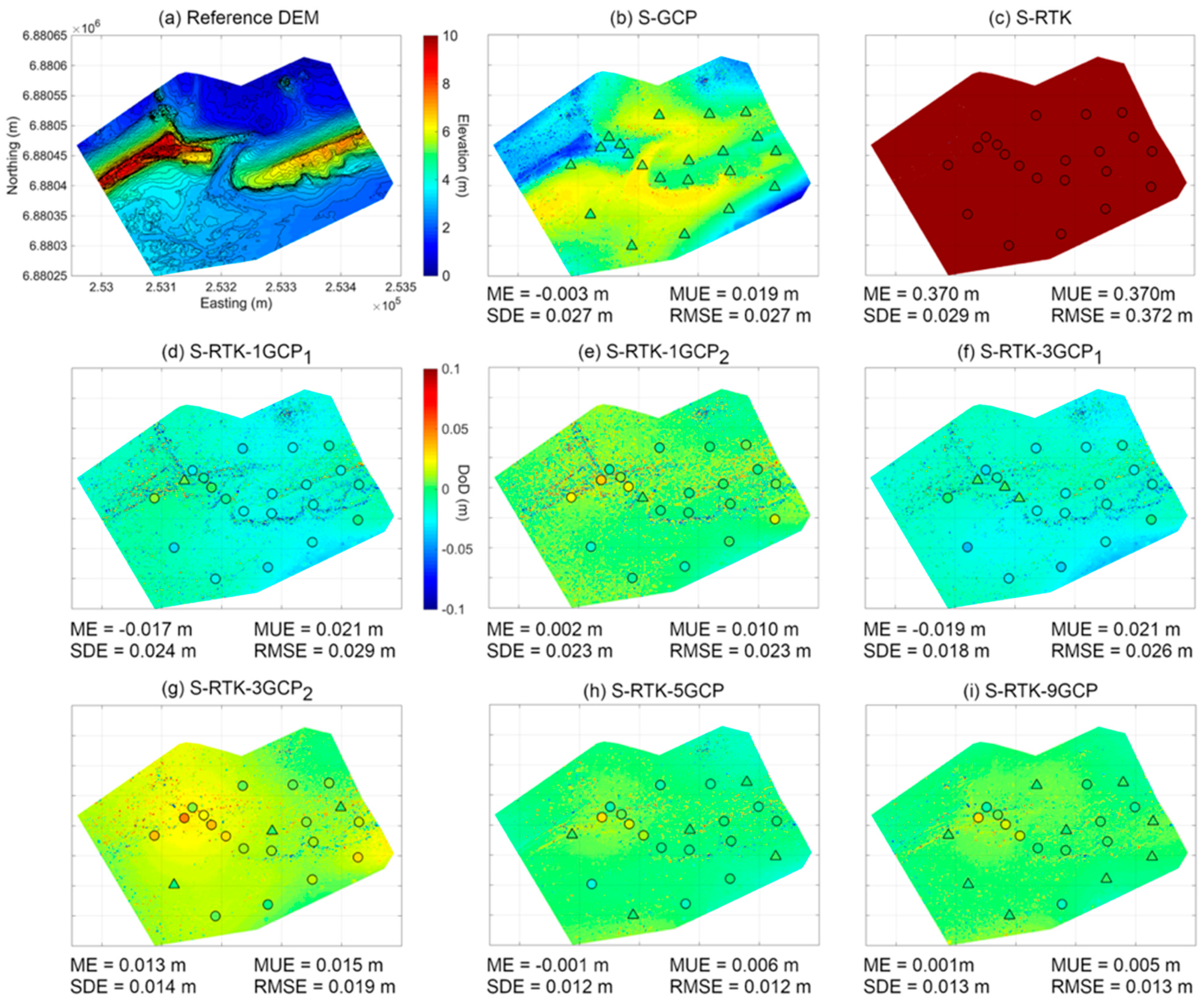
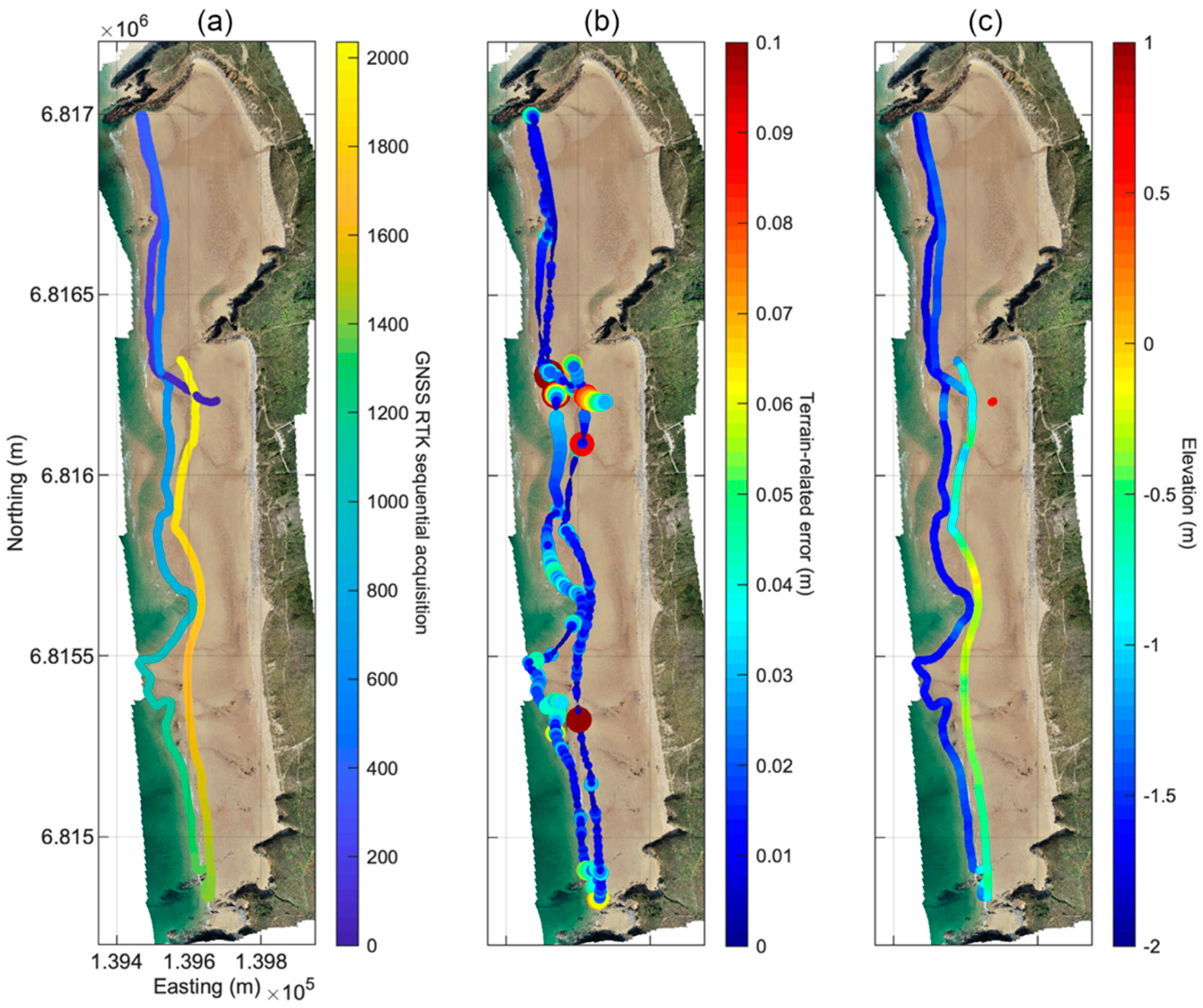
Table 1.
Overview of the field surveys and data collection for UAV–SfM photogrammetry. The tidal coefficient (20–120) represents the tide magnitude in relation to its mean.
Table 1.
Overview of the field surveys and data collection for UAV–SfM photogrammetry. The tidal coefficient (20–120) represents the tide magnitude in relation to its mean.
| Field Site Date | Tidal Coefficient (-) | Flight Count/Image Count (-) | Flying Height (m) | Overlap Along/Cross (%) | Survey Area (m2) | GSD (m/Pixel) | Target Count (Fixed Targets) (-) |
|---|---|---|---|---|---|---|---|
| Sillon de Talbert 17 November 2020 | 103 | 2/734 | 58 | 80/70 | 125,000 | 0.014 | 21 (0) |
| La Palue 17 September 2020 | 101 | 5/1407 | 106 | 80/70 | 1,320,000 | 0.026 | 30 (5) |
| La Palue 17 December 2020 | 90 | 6/1548 | 105 | 80/70 | 1,280,000 | 0.026 | 22 (3) |
| La Palue 2 March 2021 | 103 | 5/1411 | 108 | 80/70 | 872,000 | 0.025 | 19 (1) |
| La Palue 29 April 2021 | 106 | 5/1386 | 107 | 80/70 | 1,080,000 | 0.026 | 28 (6) |
Table 2.
Overview of the processing parameters and scenarios used for DEM reconstruction with Agisoft Metashape.
Table 2.
Overview of the processing parameters and scenarios used for DEM reconstruction with Agisoft Metashape.
| Processing Step/Scenario | Image Alignment | Sparse Point Cloud Filtering | Model Optimization | Dense Matching and DEM |
|---|---|---|---|---|
| Standard (High1) |
|
|
|
|
| Low | Accuracy: “low” | - | - | DEM resolution: 1 m |
| Medium | Accuracy: “medium” | - | - | DEM resolution: 1 m |
| High2 | Pair preselection: “reference” | - | - | DEM resolution: 1 m |
| Highest | Accuracy: “highest” | - | - | DEM resolution: 1 m |
| S-GCP | - | - |
| DEM resolution: 1 m |
| S-RTK | - | - | 0 GCPs/N ChkPts | DEM resolution: 1 m |
| S-RTK-GCP | - | - | N GCPs/0 ChkPts | DEM resolution: 1 m |
| S-RTK-1GCP | - | - | 1 GCPs/N−1 ChkPts | DEM resolution: 1 m |
| S-RTK-3GCP | - | - | 3 GCPs/N−3 ChkPts | DEM resolution: 1 m |
| S-RTK-5GCP | - | - | 5 GCPs/N−5 ChkPts | DEM resolution: 1 m |
| S-RTK-9GCP | - | - | 9 GCPs/N−9 ChkPts | DEM resolution: 1 m |
N is the number of photogrammetric targets available, and - stands for standard parameters.
Table 3.
Error metrics used for evaluation of measurement quality.
| Error Metric | Formula | |
|---|---|---|
| Mean Error (ME) | (1) | |
| Standard Deviation of Error (SDE) | (2) | |
| Root-Mean Square Error (RMSE) | (3) | |
| (4) | ||
| ) | (5) | |
| Mean Unsigned Error (MUE) | (6) | |
y is the measurement or observation, x the reference value and N the number of available comparisons. Horizontal and vertical bars represent the average (i.e., mean) and absolute (i.e., unsigned) values, respectively. X, Y and Z represent easting, northing and vertical (i.e., elevation) directions, respectively.
Table 4.
Vertical error evaluation for the different scenarios presented in Figure 3 using ground targets (GCPs and ChkPts) measured with RTK-GNSS. The values between brackets correspond to GCP-based error.
Table 4.
Vertical error evaluation for the different scenarios presented in Figure 3 using ground targets (GCPs and ChkPts) measured with RTK-GNSS. The values between brackets correspond to GCP-based error.
| (a) Reference DEM: S-RTK-GCP | (b) S-GCP | (c) S-RTK |
| ME = N.A. (0.000 m) | ME = N.A. (0.000 m) | ME = 0.363 m (N.A.) |
| SDE = N.A. (0.002 m) | SDE = N.A. (0.007 m) | SDE = 0.014 (N.A.) |
| (d) S-RTK-1GCP1 | (e) S-RTK-1GCP2 | (f) S-RTK-3GCP1 |
| ME = −0.019 m (0.003 m) | ME = 0.002 m (0.002 m) | ME = −0.022 m (0.001 m) |
| SDE = 0.011 (0.000 m) | SDE = 0.012 (0.000 m) | SDE = 0.010 (0.001 m) |
| (g) S-RTK-3GCP2 | (h) S-RTK-5GCP | (i) S-RTK-9GCP |
| ME = 0.016 m (0.001 m) | ME = −0.001 m (0.000 m) | ME = 0.003 m (0.000 m) |
| SDE = 0.014 (0.001 m) | SDE = 0.013 (0.002 m) | SDE = 0.012 (0.002 m) |
Table 5.
Planimetric error (X easting and Y northing) evaluation for the different scenarios presented in Figure 3 using ground targets (GCPs and ChkPts) measured with RTK-GNSS. The values between brackets correspond to GCP-based error.
Table 5.
Planimetric error (X easting and Y northing) evaluation for the different scenarios presented in Figure 3 using ground targets (GCPs and ChkPts) measured with RTK-GNSS. The values between brackets correspond to GCP-based error.
| (a) Reference DEM: S-RTK-GCP | (b) S-GCP | (c) S-RTK |
| MEX = N.A. (−0.001 m) | MEX = N.A. (0.000 m) | MEX = −0.022 m (N.A.) |
| SDEX = N.A. (0.027 m) | SDEX = N.A. (0.026 m) | SDEX = 0.037 m (N.A.) |
| MEY = N.A. (0.001 m) | MEY = N.A. (0.000 m) | MEY = 0.039 m (N.A.) |
| SDEY = N.A. (0.029 m) | SDEY = N.A. (0.027 m) | SDEY = 0.053 m (N.A.) |
| (d) S-RTK-1GCP1 | (e) S-RTK-1GCP2 | (f) S-RTK-3GCP1 |
| MEX = -0.025 m (0.025 m) | MEX = −0.019 m (−0.029 m) | MEX = −0.021 m (−0.013 m) |
| SDEX = 0.035 m (0.000 m) | SDEX = 0.038 m (0.000 m) | SDEX = 0.037 m (0.036 m) |
| MEY = 0.036 m (0.019 m) | MEY = 0.037 m (−0.014 m) | MEY = 0.044 m (−0.007 m) |
| SDEY = 0.053 m (0.000 m) | SDEY = 0.049 m (0.000 m) | SDEY = 0.048 m (0.028 m) |
| (g) S-RTK-3GCP2 | (h) S-RTK-5GCP | (i) S-RTK-9GCP |
| MEX = −0.019 m (0.003 m) | MEX = −0.009 m (0.003 m) | MEX = 0.003 m (−0.003 m) |
| SDEX = 0.037 m (0.022 m) | SDEX = 0.039 m (0.018 m) | SDEX = 0.042 m (0.021 m) |
| MEY = 0.026 m (0.005 m) | MEY = 0.004 m (0.009 m) | MEY = −0.009 m (0.004 m) |
| SDEY = 0.047 m (0.010 m) | SDEY = 0.047 m (0.016 m) | SDEY = 0.050 m (0.014 m) |
Table 6.
Effect of changing the image alignment accuracy setting during sparse DEM reconstruction at La Palue field site in terms of processing time, number of tie points (before and after filtering) and measurement error. Deviations between photogrammetric models (1 m resolution) and GNSS-RTK survey points, from which vertical error statistics are extracted, are presented in Figure 5.
| (a) Low | (b) Medium | (c) High1 | (d) High2 | (e) Highest | |
| Alignment time | 27 min | 43 min | 105 min | 2721 min | 105 min |
| Initial tie points | 567,716 | 1,918,509 | 2,102,195 | 1,967,440 | 2,482,173 |
| Final tie points | 79,909 | 412,200 | 435,657 | 402,828 | 320,413 |
| Error statistics | ME = 0.000 m | ME = −0.001 m | ME = 0.000 m | ME = −0.002 m | ME = −0.004 m |
| MUE = 0.096 m | MUE = 0.038 m | MUE = 0.031 m | MUE = 0.033 m | MUE = 0.045 m | |
| SDE = 0.125 m | SDE = 0.049 m | SDE = 0.042 m | SDE = 0.044 m | SDE = 0.062 m | |
| RMSE = 0.125 m | RMSE = 0.049 m | RMSE = 0.042 m | RMSE = 0.044 m | RMSE = 0.062 m | |
| Max = 0.368 m | Max = 0.145 m | Max = 0.117 m | Max = 0.144 m | Max = 0.213 m |
Table 7.
Evaluation of depth filtering during dense DEM reconstruction at La Palue field site. Except for the reference DEM using no depth filtering, for which errors are estimated in comparison to 1381 RTK-GNSS survey points, vertical error statistics are the result of intercomparing DEMs with the reference DEM. All DEMs evaluated were reconstructed using “High” image alignment accuracy (Figure 5c) and “High” reconstruction quality for sparse and dense DEM reconstructions, respectively (cf. explanations in the text). Evaluations were performed using 0.1 m resolution DEMs.
| (a) Reference DEM | (b) Mild | (c) Moderate | (d) Aggressive |
| ME = 0.001 m | ME = 0.000 m | ME = −0.001 m | ME = −0.001 m |
| MUE = 0.027 m | MUE = 0.003 m | MUE = 0.005 m | MUE = 0.005 m |
| SDE = 0.033 m | SDE = 0.072 m | SDE = 0.084 m | SDE = 0.084 m |
| RMSE = 0.033 m | RMSE = 0.072 m | RMSE = 0.084 m | RMSE = 0.084 m |
| Maximum = 0.186 m | Maximum = 76.23 m | Maximum = 77.33 m | Maximum = 77.33 m |
Publisher’s Note: MDPI stays neutral with regard to jurisdictional claims in published maps and institutional affiliations. |
© 2022 by the authors. Licensee MDPI, Basel, Switzerland. This article is an open access article distributed under the terms and conditions of the Creative Commons Attribution (CC BY) license (https://creativecommons.org/licenses/by/4.0/).
Share and Cite
MDPI and ACS Style
Bertin, S.; Stéphan, P.; Ammann, J. Assessment of RTK Quadcopter and Structure-from-Motion Photogrammetry for Fine-Scale Monitoring of Coastal Topographic Complexity. Remote Sens. 2022, 14, 1679. https://doi.org/10.3390/rs14071679
AMA Style
Bertin S, Stéphan P, Ammann J. Assessment of RTK Quadcopter and Structure-from-Motion Photogrammetry for Fine-Scale Monitoring of Coastal Topographic Complexity. Remote Sensing. 2022; 14(7):1679. https://doi.org/10.3390/rs14071679
Chicago/Turabian StyleBertin, Stéphane, Pierre Stéphan, and Jérôme Ammann. 2022. "Assessment of RTK Quadcopter and Structure-from-Motion Photogrammetry for Fine-Scale Monitoring of Coastal Topographic Complexity" Remote Sensing 14, no. 7: 1679. https://doi.org/10.3390/rs14071679
Note that from the first issue of 2016, this journal uses article numbers instead of page numbers. See further details here.