Variations in Flow Patterns in the Northern Taiwan Strait Observed by Satellite-Tracked Drifters

Abstract

This study investigates the variations in flow patterns in the northern Taiwan Strait in summer using high-frequency (HF) radar measurements, satellite-tracked drifter trajectories and numerical models. There is an obvious interaction between intra-diurnal tides and ocean currents in northwestern Taiwan. When the tide changes between high tide and low tide, the change in direction of the nearshore flow occurs before the change in the offshore flow. Drifter trajectories show that there are three different drifting paths in the Taiwan Strait in summer. One path is along the west coast of Taiwan from the southwest coast to the northeast coast. Another path is the same as the first one but leads northward to the East China Sea instead of eastward to the northeast coast of Taiwan. The other path exists along the west coast of Taiwan, some distance out, after being deflected by the bottom ridge. The regional ocean modeling system model was used in this study to clarify the influencing factors that lead to these three paths. The results of multiple simulations and HF radar data indicate that the bifurcation of the first two drift paths in northwestern Taiwan is caused by ebb and flood tide transitions. The different routes of the latter two paths are due to the significant speed difference between the nearshore current and the offshore current approximately 45 km from the coast.

1. Introduction

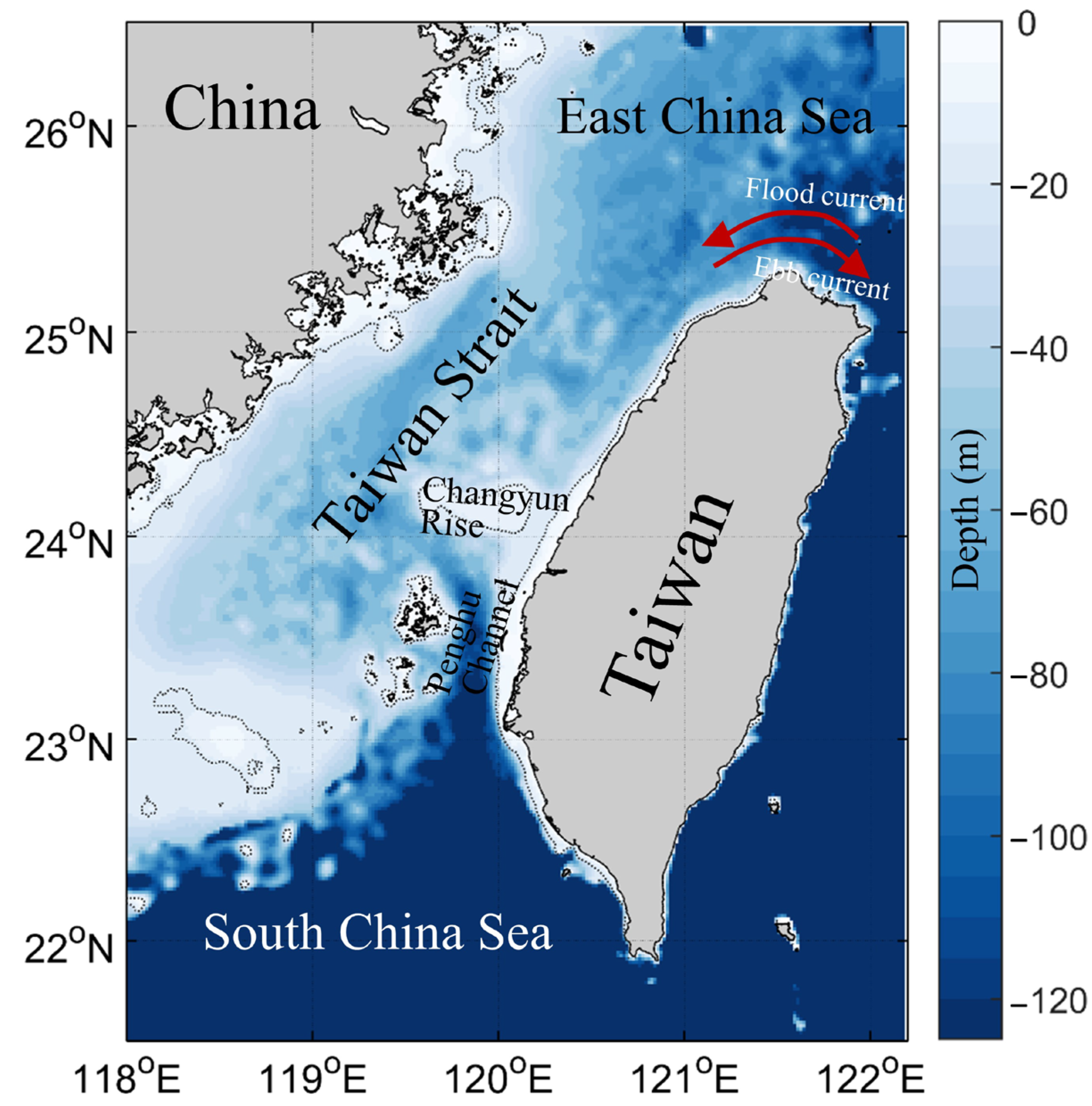
The Taiwan Strait (TS), located between China and Taiwan, is a narrow passage that connects to the South China Sea (SCS) in the south and the East China Sea (ECS) in the north. It has been an important waterway since ancient times. As shown in Figure 1, TS is a shallow strait about 60 m in depth on average. There is a deeper water channel in the TS, named Penghu Channel, located along the southwest coast of Taiwan; the bottom ridge of Changyun Rise (CYR) is north of it. The currents in the TS may be influenced by monsoon and long-term winds. Wind fields in the TS are dominated by the East Asian monsoon, which is southwesterly from May to August and northeasterly from September to April [1]. Previous studies mentioned that seasonal variations in volume transport in the TS are related to the reversal of the monsoon [2] and wind stress along the TS [3]. Additionally, the TS is strongly affected by other ocean currents from southern water [4]. These ocean currents include the remnants of the SCS warm current from the SCS and a branch of Kuroshio from the Luzon Strait [5,6]. Tidal currents also contribute to the flow in the Taiwan Strait [7]. In short, the currents in the TS are influenced by the complex topography, the monsoon wind, tides, and ocean currents from south of the TS.

Penghu Channel, which is the deepest passage in the TS, causes most of the water to converge and flow northward. Previous observations from shipboard ACDP show that the Penghu Channel is the major pathway for northward current in the TS, and the velocity is about 1 m/s after removing the tidal effect in the upper 50 m during summer [8]. Therefore, the Penghu Channel is an important entrance to the TS. In addition, the effect of the semidiurnal tide is quite significant in the TS. In the flood tide period, the water enters through the south and north entrances of the TS, and it leaves in the ebb tide period. The tidal range in the northern TS is larger than that in the southern TS [9]. Additionally, the tidal current is larger on the Taiwanese coast than on the mainland coast. The maximum amplitude is 0.80 m/s at the two entrances, and the minimum amplitude is 0.20 m/s in the middle of the TS [10]. Due to the strong tidal effect, the currents at the two entrances of the TS must be affected by the tidal currents. The sea surface temperature and chlorophyll could be moved westward and turned eastward with tidal current according to satellite images [11]. It is well known that the main current flows northward in the TS during summer. However, this phenomenon is based on long-term observations. The above results indicate that the tide, which changes between flood and ebb tides twice a day, might cause significant intra-diurnal variability in the flow pattern, especially at the north end of the TS.

Most previous studies observed flow patterns based on Eulerian descriptions. However, it is hard to depict the path of flow over time. On the contrary, satellite-tracked drifters can provide direct evidence to present the flow pattern in Lagrangian descriptions. A previous study divided the near-surface circulation into four kinds of patterns in winter based on the trajectories of drifters collected before 2007 [12]. In summer, most drifters travel northward through the TS to the ECS. It seems that the flow pattern in the TS was a steady northward flow [12]. However, after passing through the Penghu Channel at a high speed, the seawater immediately encounters the shallow area of CYR. With the influence of complex topography and the strong tidal effect, they may cause complicated changes in local flow fields. Therefore, if the variations in flow patterns in the northern TS can be clarified, it can assist in navigation safety, rescue, or tracking of marine debris. To understand the detailed effects of monsoon, tide, and current interactions, we used satellite-tracked drifters and HF radar to analyze variations in flow patterns and numerical models to find the causes of different current paths in the TS.

The remainder of this paper is organized as follows. Section 2 describes the data and methods. Section 3 presents the characteristics of surface currents with HF radar data and drifters. Section 4 presents the simulations of the nearshore current during summer under several conditions. Section 5 discusses the factors that cause the different current paths. Finally, Section 6 summarizes the main results.

2. Data and Methodology

2.1. High-Frequency Radar Data

The ocean surface current data used in this study are one-hour temporal resolution and 10 km spatial resolution data provided by the Taiwan Ocean Radar Observing System (TOROS) using the Coastal Ocean Dynamics Application Radar (CODAR) developed by the Taiwan Ocean Research Institute (TORI). There are 19 CODAR stations, including 13 sets of long-range 5 MHz systems and six sets of 13/24 MHz systems along the coast of Taiwan Island with the date period from January 2013 to December 2020. Unfortunately, some of the CODAR stations stopped supplying data after December 2020 because of the problems with devices and the lack of components. These high-frequency radars work on the principle of radio wave backscatter and Bragg scattering by analyzing the Doppler frequency shift from the first-order Doppler peak of the sea-echo reflected from the ocean surface. The Doppler frequency shift is due to the ocean current and gravity wave velocities [13]. The phase speed of the gravity wave in deep water is √(gλ/2π), where g is the gravitational acceleration, and λ is the wavelength of gravity waves. Due to the Bragg scattering, the wavelength of the gravity wave measured by the CODAR is half the radar wavelength. The ocean velocity in the radial direction is calculated based on the difference between the measured velocities of radar and gravity waves. A single radar can only measure the radial velocity; the current vectors need to be determined by multiple CODAR sites.

2.2. Satellite-Tracked Drifter Trajectories

Satellite-tracked drifter trajectory data were downloaded from the National Oceanic and Atmospheric Administration (NOAA) Global Drifter Program database (GDP database) [14]. After the quality control and optimal interpolation procedures by the Drifter Data Assembly Center at Atlantic Oceanographic and Meteorological Laboratory (AOML), the data were interpolated for 6-h intervals. This dataset includes position (longitude, latitude, and time), sea surface temperature, and velocity. The drifter drogue is 15-m long and the bottom of the drogue is about 20-m deep [15]. A total of 30 trajectories were collected from March 1989 to December 2020. These started at the SCS, passed through the Penghu Channel, and entered the ECS north of Taiwan.

2.3. Numerical Model

This study employed the Regional Ocean Modeling System (ROMS) model to better understand the dynamic process and physical mechanism of the coastal flow field in the TS. ROMS is a three-dimensional, realistic bathymetry and free-surface ocean model used to simulate mesoscale and small-scale ocean phenomena around Taiwan [16,17]. The model domain was 118–124°E and 20–26.5°N, using a horizontal resolution of 0.05°. Vertically, there are ten sigma coordinate levels. The bathymetry of the model was extracted from the ETOPO1 database. The initial conditions of the model were set to zero and forced by climatological data from the Comprehensive Ocean-Atmosphere Data Set with open boundaries. The amplitudes and phases of the tidal constituents were derived from Oregon State University global models of ocean tides, TPXO7 [18], along with ten parameters (M2, S2, N2, K2, K1, O1, P1, Q1, Mf, and Mm). The model period was 30 days. The temporal resolution of the model output was one hour. The area in the Kuroshio region east of Taiwan that is in deeper water was not discussed in this study because the simulation focused on the continental shelf in shallow water.

3. Characteristics of Surface Currents in the North Side of TS

3.1. Tide-Current Interaction Observed by HF Radar Data

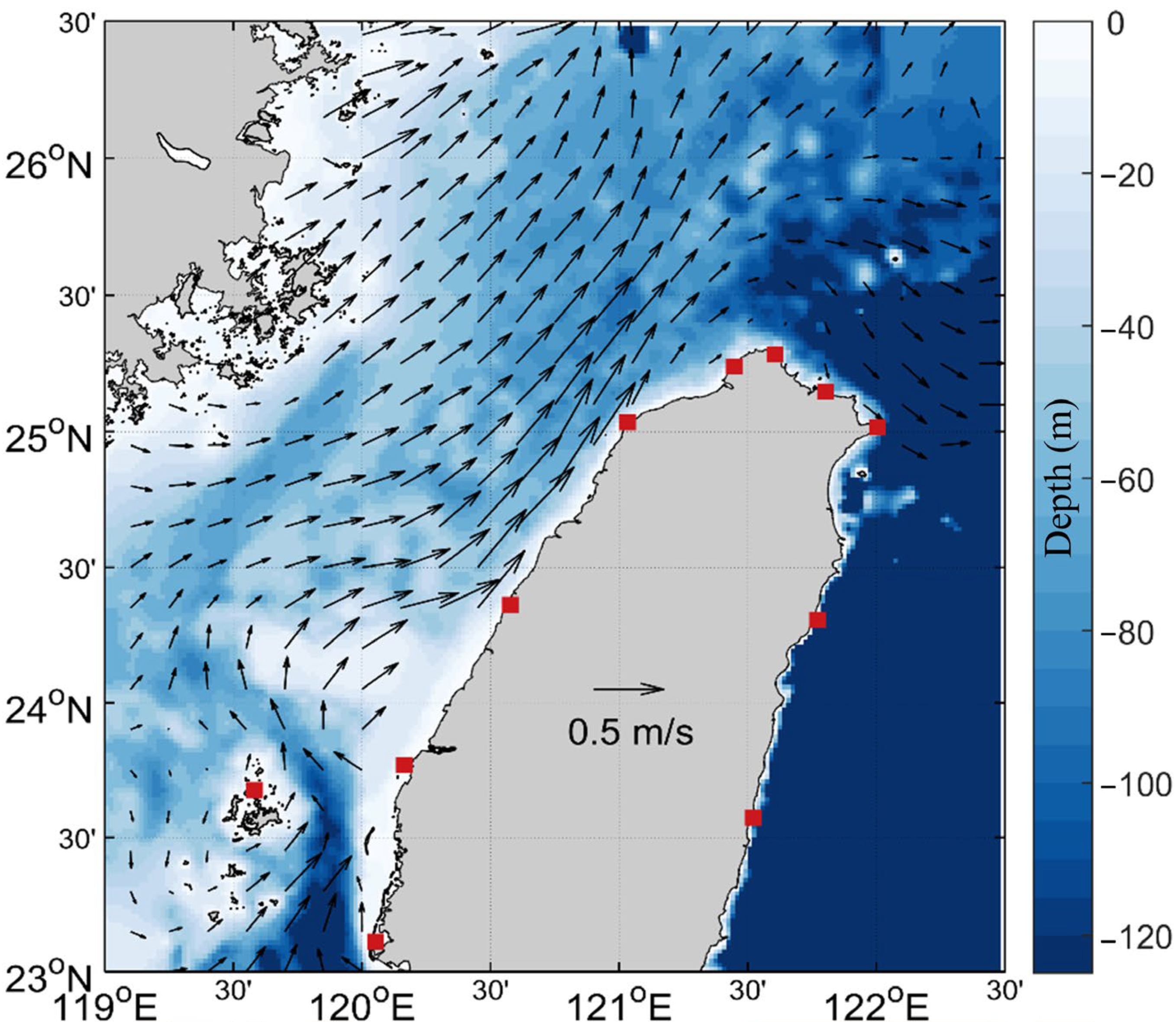
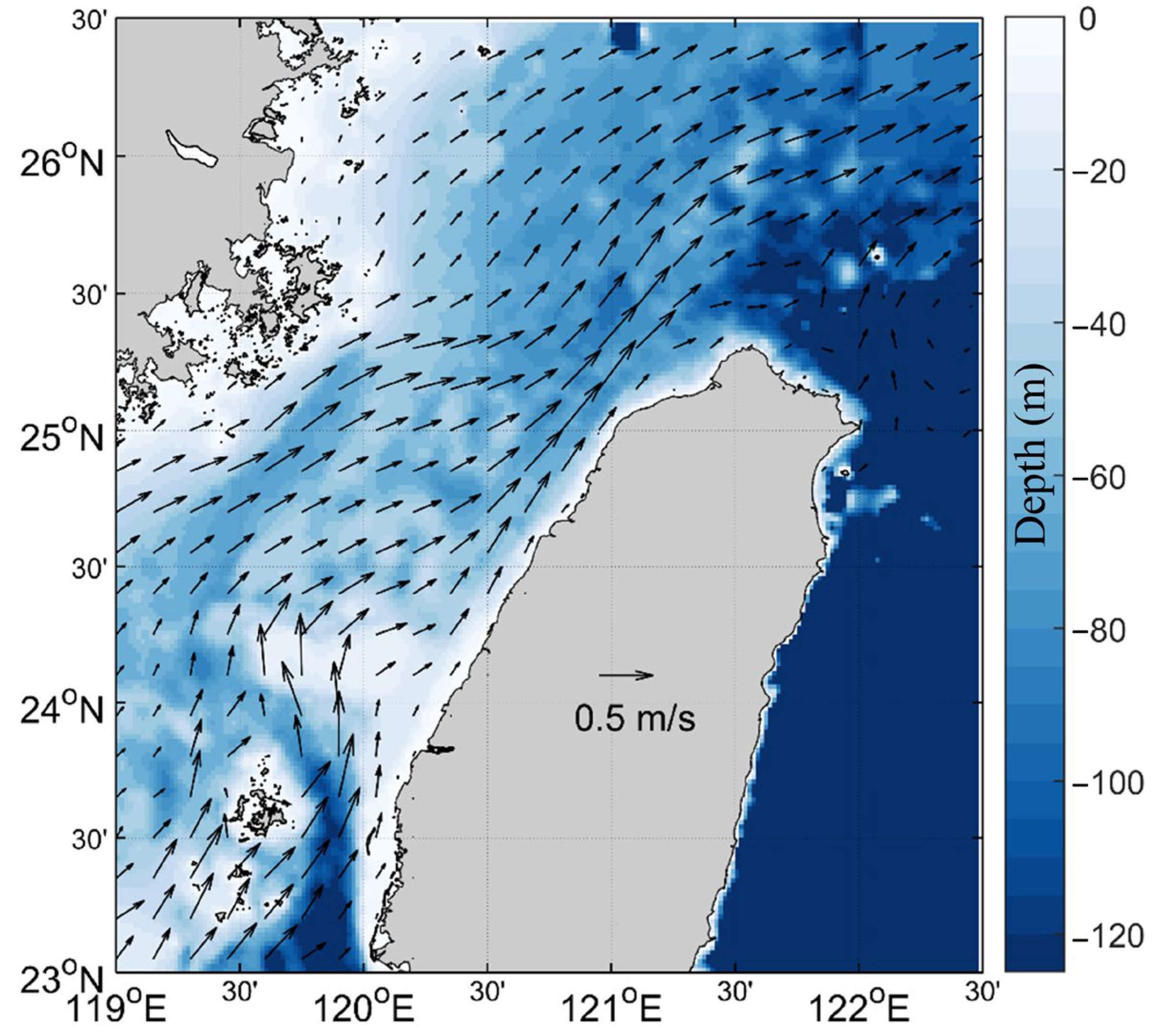
It is worth noting that the flow direction of the ebb tidal current at the north end of the TS was the same as the background current in summer, but the flood tidal current faced the opposite direction (see Figure 1). Therefore, there was complicated intra-diurnal variability in currents at the north end of the TS during the tidal period. The intra-diurnal variability in surface currents was hard to measure continuously by either satellite altimetry or ship-based sensors. However, coastal HF radar stations could provide high temporal and spatial resolution ocean surface current data around Taiwan. It is possible to observe the variations in nearshore current with the tidal effect; even the tide-current interaction in the TS. Figure 2 shows the average flow fields of the CODAR data in the summer (June to August) of 2017. Due to the southwest monsoon winds and narrow terrain, the background flow field of the TS was dominated by the northeastward current. After passing through the Penghu Channel, the ocean current was deflected by the bottom ridge of CYR and then continued to flow northward in the middle of the TS and entered the ECS. Interestingly, there was a current branch before the TS current entered the ECS. One of the tributaries flowed to the south of the ECS, while the other deflected eastward at a slower speed.

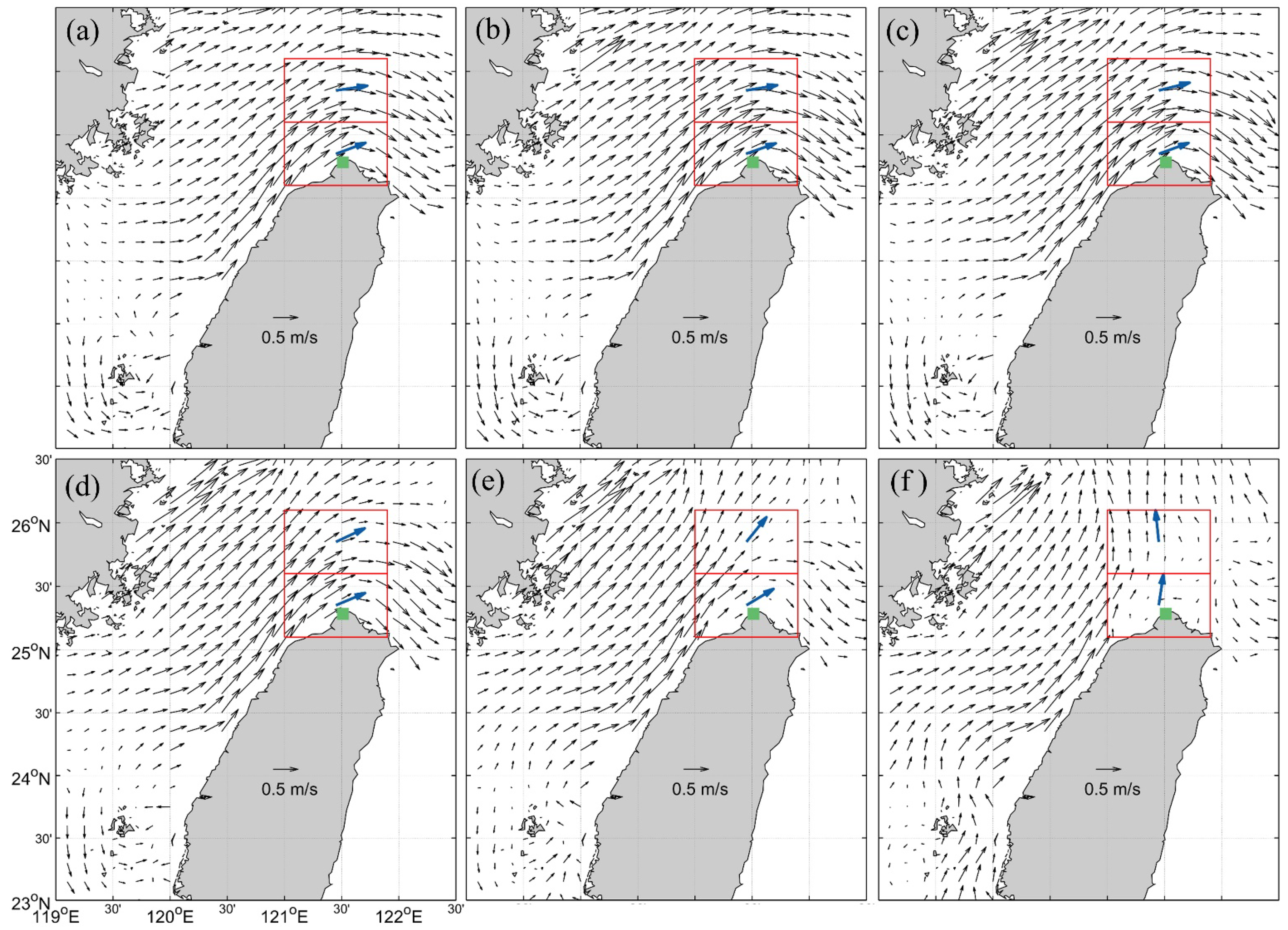
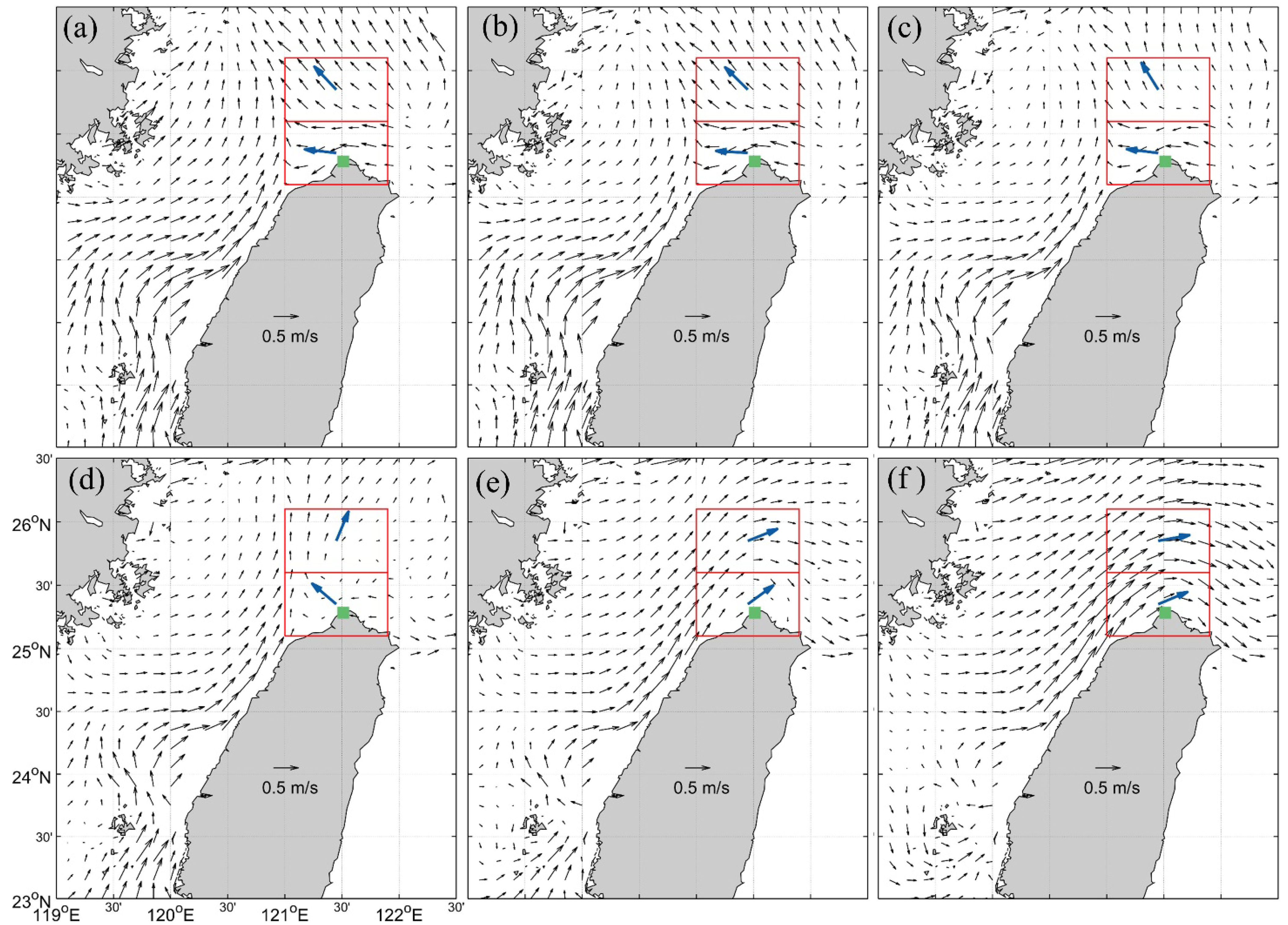
In this study, we calculated six-hour average flow fields during different tidal periods based on the Linshanbi tidal station (green square in Figure 3 and Figure 4), which was established by the Central Weather Bureau of Taiwan. Figure 3a shows the average flow field of the six-hour period after high tide in the summer of 2017. Figure 3b shows the average flow field for the six-hour period from one hour after high tide. Figure 3f shows the average current of the six-hour period starting from five hours after high tide in the summer of 2017. As in Figure 3 and Figure 4 show the average flow fields of the six-hour period after low tide in the summer of 2017. According to short-time average flow fields during different tidal periods, there was complicated intra-diurnal variability. In particular, when the period of average current spanned low tide, there was obvious tide–current interaction during the flood tide, which flowed in the opposite direction to the average flow fields in the TS during summer (Figure 3e,f and Figure 4a–d). We also divided the ocean above northern Taiwan into two areas to explore the changes in flow directions nearshore and offshore.

The flow speeds nearshore and offshore during the ebb period could reach 0.52 and 0.41 m/s, respectively (Figure 3b), and the flow directions were almost the same. On the other hand, because the direction of flow in the TS in summer was opposite to that of the flood current, the flow speeds nearshore and offshore were only 0.26 and 0.23 m/s, respectively (Figure 4b), and flowed in different directions. Furthermore, the average flow field began to change in the six-hour periods starting from four hours after high tide (Figure 3e) and three hours after low tide (Figure 4d). As shown in Figure 3e, the offshore current began to turn northward, while the nearshore current still flowed eastward. The flow speeds nearshore and offshore were only 0.24 and 0.20 m/s, respectively. In Figure 4d, the background flow in summer gradually dominated the flow field when the flood current weakened. At this time, the flow speeds nearshore and offshore were only 0.08 and 0.11 m/s, respectively.

Table 1. The average speed of surface current within the red frame of Figure 3 and Figure 4.

		Average Velocity of Red Frames in Figure 3 and Figure 4 (m/s)
		(a)	(b)	(c)	(d)	(e)	(f)
Figure 3	offshore	0.37	0.42	0.38	0.29	0.20	0.18
	nearshore	0.44	0.52	0.51	0.41	0.24	0.08
Figure 4	offshore	0.25	0.23	0.16	0.11	0.20	0.32
	nearshore	0.22	0.26	0.20	0.08	0.15	0.33

shows the details of flow speeds north of Taiwan displayed in Figure 3 and Figure 4.

To sum up, in summer, the velocity of the nearshore current was faster than that of the offshore current during the flood tide period in northern Taiwan, but there was no obvious difference during the ebb tide period. Additionally, the flow speed during the ebb period was about twice as fast as during the flood period. In addition, the flow direction started to change when the tidal period crossed high tides or low tides. At the same time, the flow speed decreased significantly.

3.2. Flow Paths Observed by Drifter Trajectories

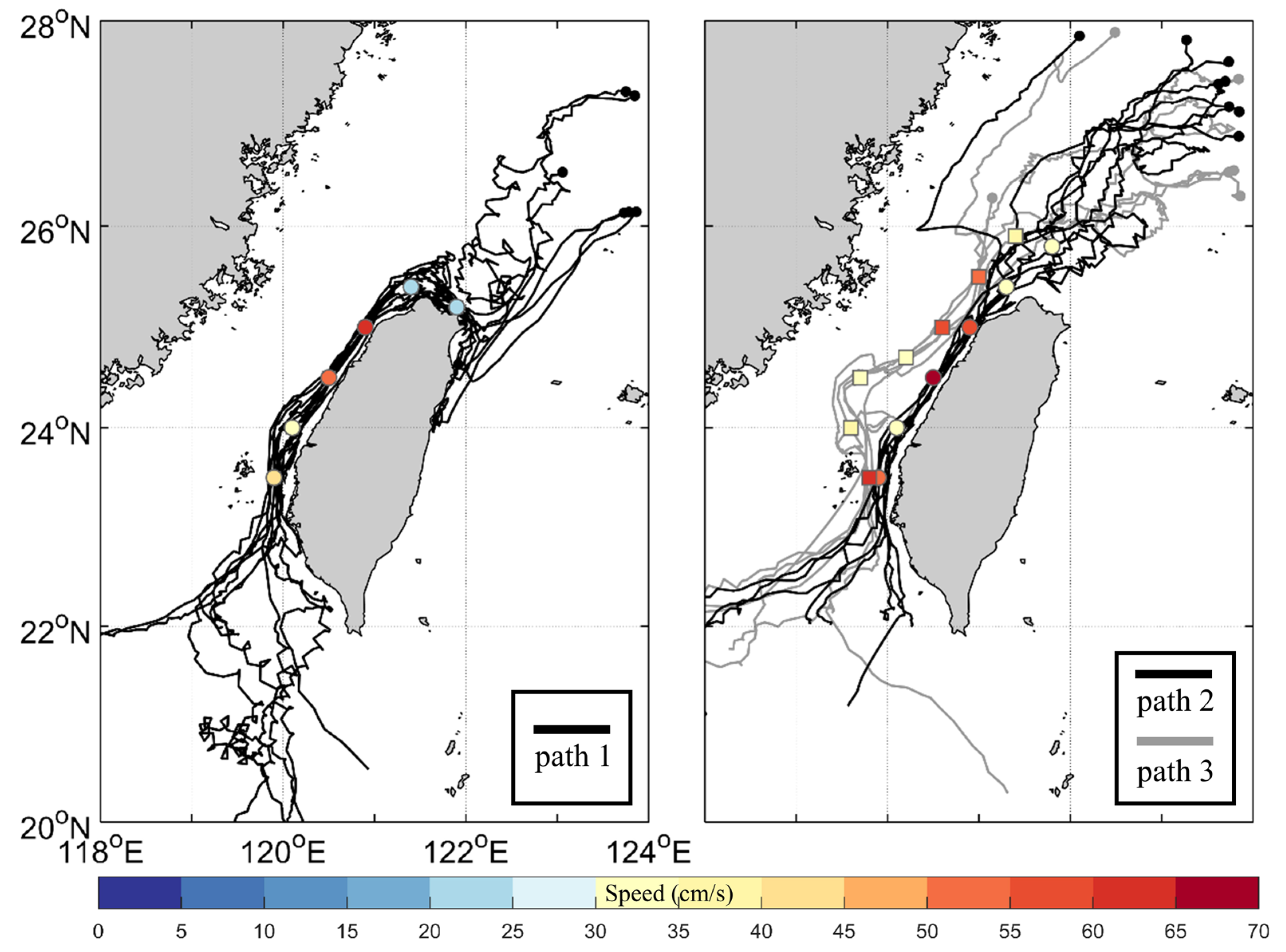
This study monitored 30 drifters that drifted northward through the Penghu Channel in the whole GDP database as of December 2020, and most of them drifted through the TS between May and August. There were 24 drifters whose drifting paths could be classified into three types (Figure 5) based on the trajectories; except for six drifters with strange drifting paths that were hard to classify, the classification conditions were as follows:

Path 1: (1) The drifters passed through the Penghu Channel and across the bottom ridge. (2) Then, they drifted close to the west coast of Taiwan. (3) Additionally, they drifted eastward to the northeast coast of Taiwan.

Path 2: (1) The drifters passed through the Penghu Channel and across the bottom ridge. (2) Then, they drifted close to the west coast of Taiwan. (3) They drifted to the south ECS instead of eastward to the northeast coast of Taiwan.

Path 3: (1) The drifters passed through the Penghu Channel and bypassed the bottom ridge. (2) They drifted along the west coast of Taiwan at a distance from the coast. (3) They drifted to the south ECS instead of eastward to the northeast coast of Taiwan.

Figure 5. Trajectories of several satellite-tracked drifters that drifted clockwise around Taiwan. The black and gray circles represent the drifter destinations. The colored patches represent the average speeds of the drifting paths.

Figure 5. Trajectories of several satellite-tracked drifters that drifted clockwise around Taiwan. The black and gray circles represent the drifter destinations. The colored patches represent the average speeds of the drifting paths.

There were three different flow patterns driving drifters in the TS during summer. Path 1 shows these drifters drifted through the Penghu Channel with an average speed of 0.41 m/s. Then they drifted across the sea surface of the bottom ridge of CYR at 0.32 m/s and drifted northward along the western coast of Taiwan at 0.54–0.65 m/s. When these drifters arrived at the northwestern Taiwanese coast, they slowed down and deflected eastward to the northeast end of Taiwan at 0.20–0.22 m/s. Path 2 was similar to path 1. These drifters also drifted through the Penghu Channel and across the sea surface of the bottom ridge at 0.53 m/s and 0.57–0.68 m/s, respectively. However, they continued to drift northward to the ECS at 0.35 m/s instead of deflecting northward to the northeast of Taiwan. Path 3 was quite different from paths 1 and 2. These drifters drifted through the Penghu Channel with an average speed of 0.63 m/s. Notice that these trajectories were farther away from the west coast of Taiwan than paths 1 and 2. They did not cross the bottom ridge but bypassed it to the middle of the TS at 0.35–0.40 m/s. These drifters drifted to the ECS at 0.33–0.60 m/s through the middle of the TS, far from the coast of Taiwan.

In summary, we found that there were ten, eight, and six drifter trajectories that drifted along paths 1, 2, and 3, respectively, though a total of 30 drifters passed through the Penghu Channel in this study. This means that the probabilities of drifters using the three drifting paths were 33.3%, 26.7%, and 20.0%, respectively. The drifters that flowed along path 1 drifted along the coast of Taiwan until they arrived at the northeast end of Taiwan. Path 2 was similar to path 1 but extended to the ECS instead of deflecting eastward. The destination of path 3 was the same as that of path 2, but path 3 was farther from the coast than that of path 2.

4. Simulations of Nearshore Current in the TS during Summer

In the previous section, we found that there were three types of different flow patterns observed by drifters in the TS. The difference in destination between path 1 and path 2 may be caused by the tide–current interaction. As shown in Figure 3a–d, the flow direction of the ebb tidal current is the same as that of the background current in the northern TS, and this flow direction is similar to the direction of path 1. However, the flow direction of the offshore current started to flow northeastward during the next six-hour period (Figure 3e). In this period, the nearshore current was similar in direction to path 1 but the offshore current was more like path 2. These results show that the transition of ebb and flood tides could cause a different current path in the northern TS. Most of the drifters were drifting through the TS between May and August (summer) (Figure 5). To further explore the influences of tides on ocean surface currents in the TS, the ROMS ocean model was used to simulate the flow field in summer in the TS.

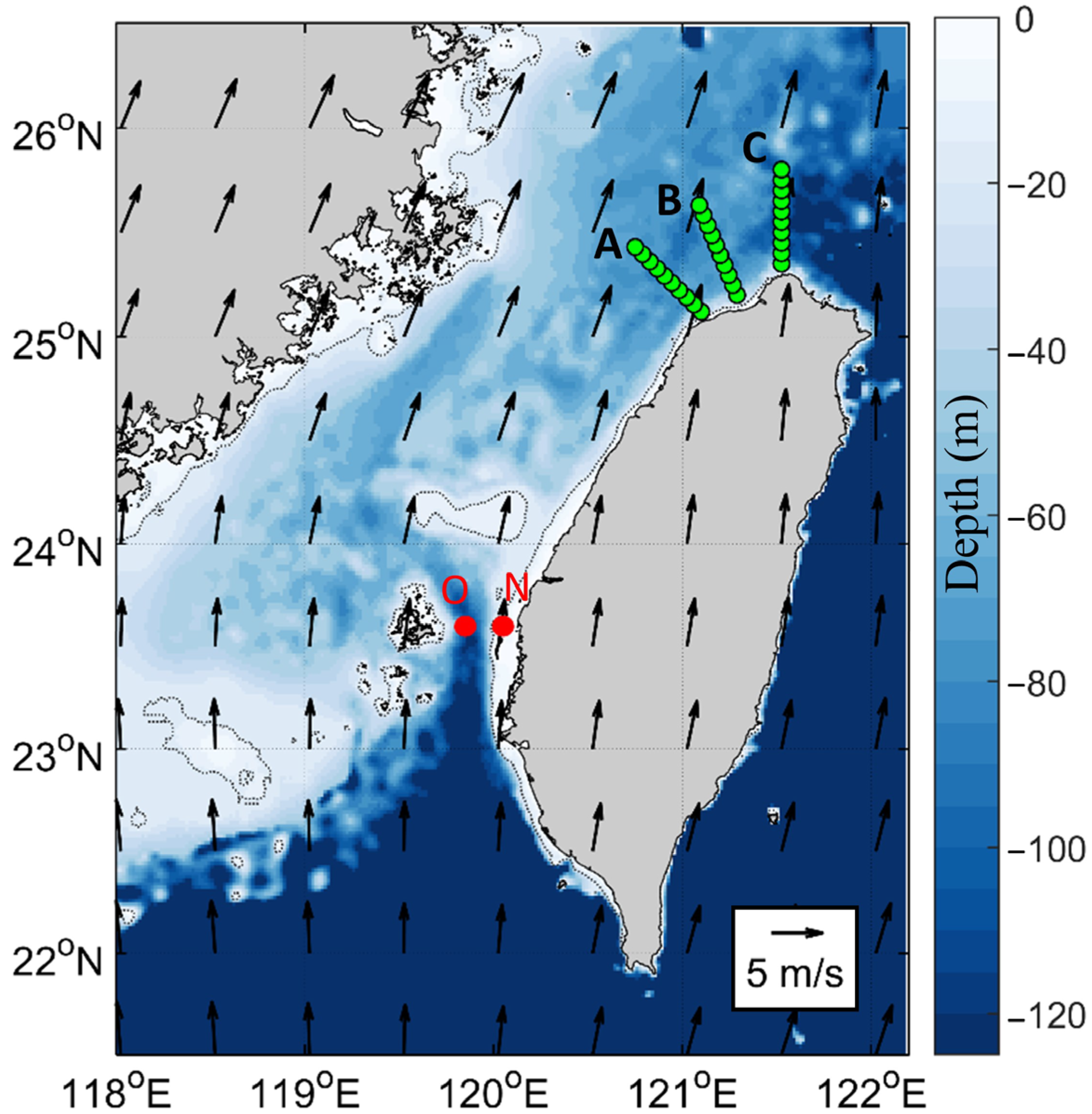
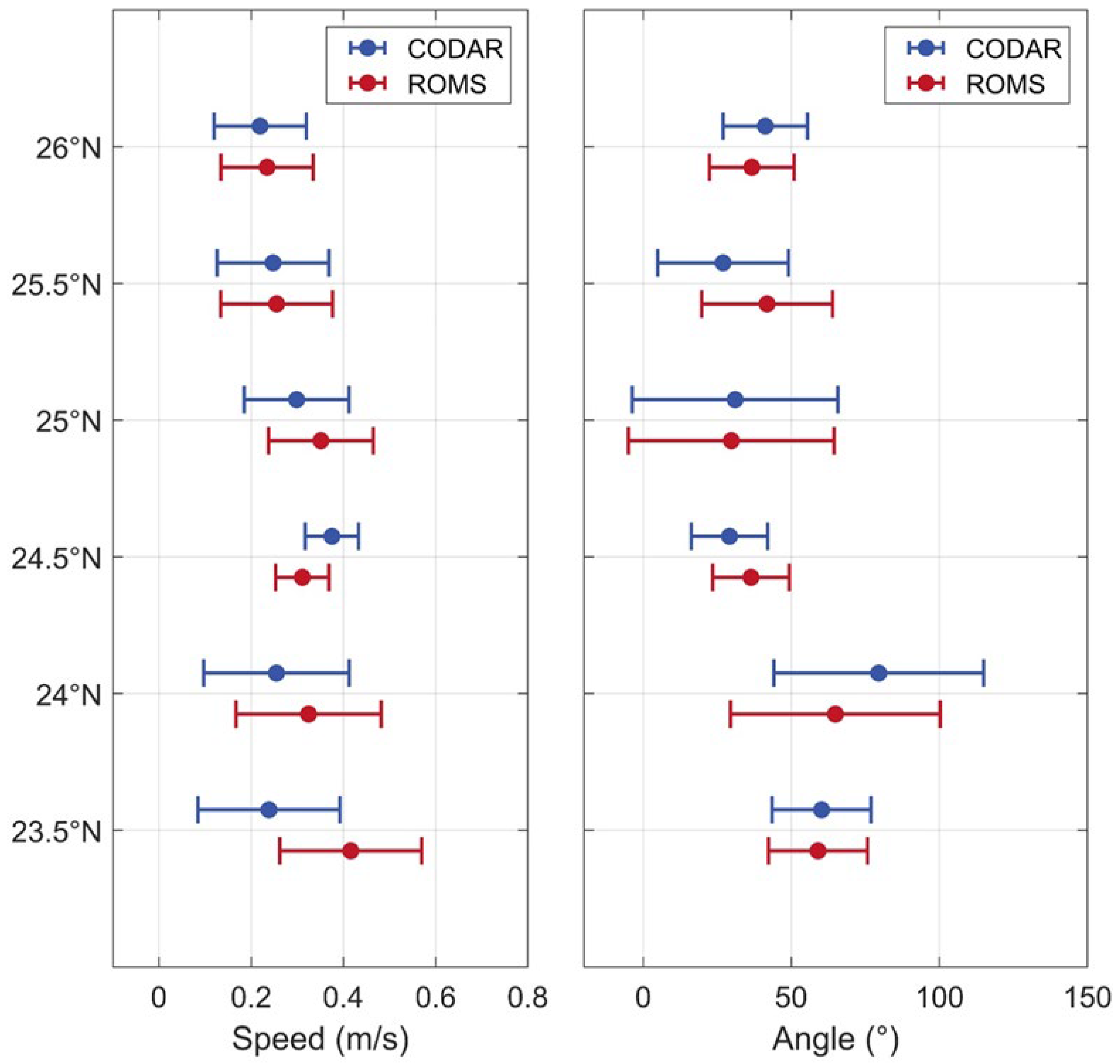
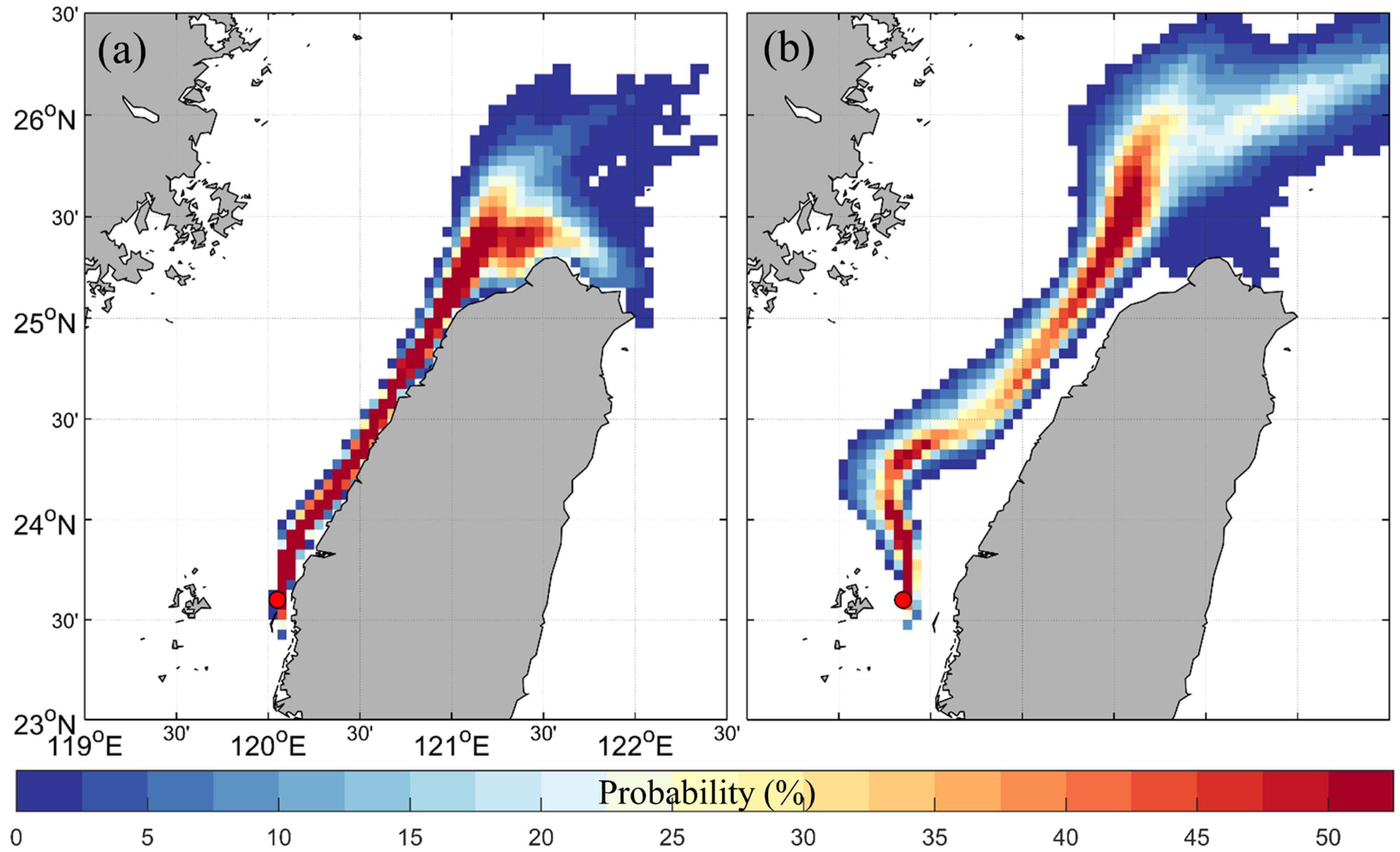
This study used the summer climatological wind to drive the ocean current with open boundaries in the model (Figure 6). Figure 7 presents the average surface flow fields of the ROMS simulation, and Figure 8 shows comparisons of flow speed and direction between ROMS outputs and CODAR observations from 23.5°N–26°N and 119.5°E–122°E. The average surface flow field was divided into five latitude bands at every 0.5° of latitude. The results show that the flow fields of ROMS were close to the average flow fields of CODAR in most latitude bands. To intuitively present the modeled flow fields, we used the particle tracking function in ROMS to simulate drifter trajectories. Two points in the Penghu Channel, the nearshore point (23.60°N, 120.05°E) and the offshore point (23.60°N, 119.85°E), were selected to release the floats (Figure 6). When the model was stable (after 72 h), the simulated floats were continuously released every hour for 360 h. Therefore, 360 simulated floats were released at each point. The depth of release for the simulated floats was 10 m because there was a 15-m-long drogue under the satellite-tracked drifters. Figure 9 shows the probability density distribution of the simulated floating trajectories released from the Penghu Channel. We found that the trajectories of the floats were affected by the distance from the starting position to the shore. The simulated floats that were released from the nearshore position (point N in Figure 6) could drift northward along the west coast of Taiwan. More than 40% of the floats drifted eastward to the north of Taiwan, and about 35% of the floats drifted northward to the ECS. The remaining floats were stopped by the coast. However, the simulated floats released from the offshore position (point O in Figure 6) kept their distance from the coast of Taiwan and drifted northward until arriving in the ECS. More than 50% of the floats drifted northward to the ECS, whereas less than 5% drifted to the north of Taiwan. The remaining floats were stopped by the coast.

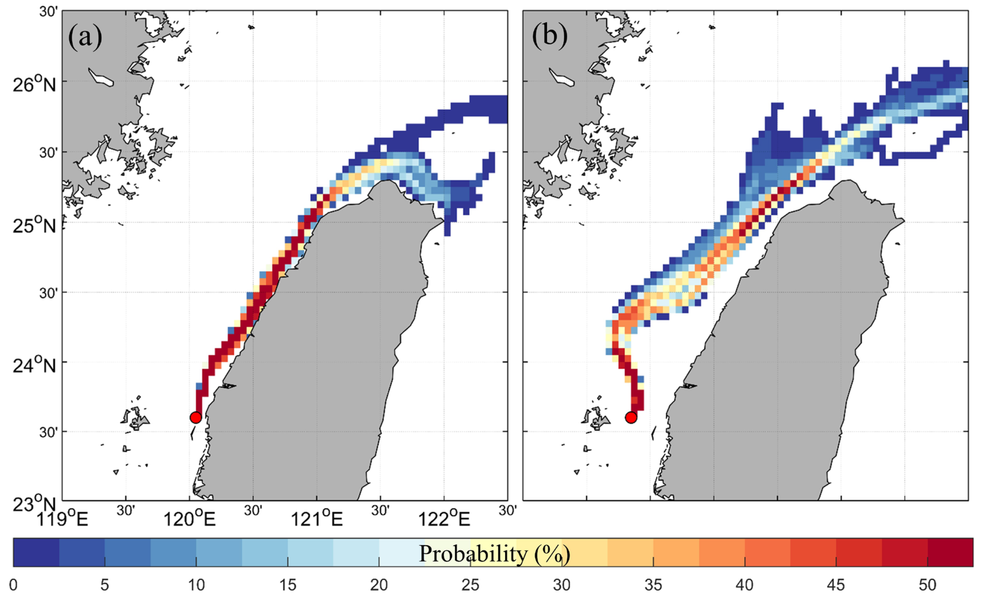
To confirm the influence of tides on the ocean current in the TS, we performed another simulation with the same model settings as above but without the tidal forcing. The simulated floats were also deployed at nearshore and offshore points in the Penghu Channel, and the probability density distributions are shown in Figure 10. The results show that the trajectories of simulated floats were similar regardless of whether the tidal forcing was turned on or off before the floats flowed into the ECS. However, there was a significant difference after the floats passed through the TS. More than 30% of the floats released from the nearshore drifted eastward to the north end of Taiwan, but there were a few cases of floats drifting northward to the ECS. The simulated floats released from offshore drifted northeastward after passing northwestern Taiwan.

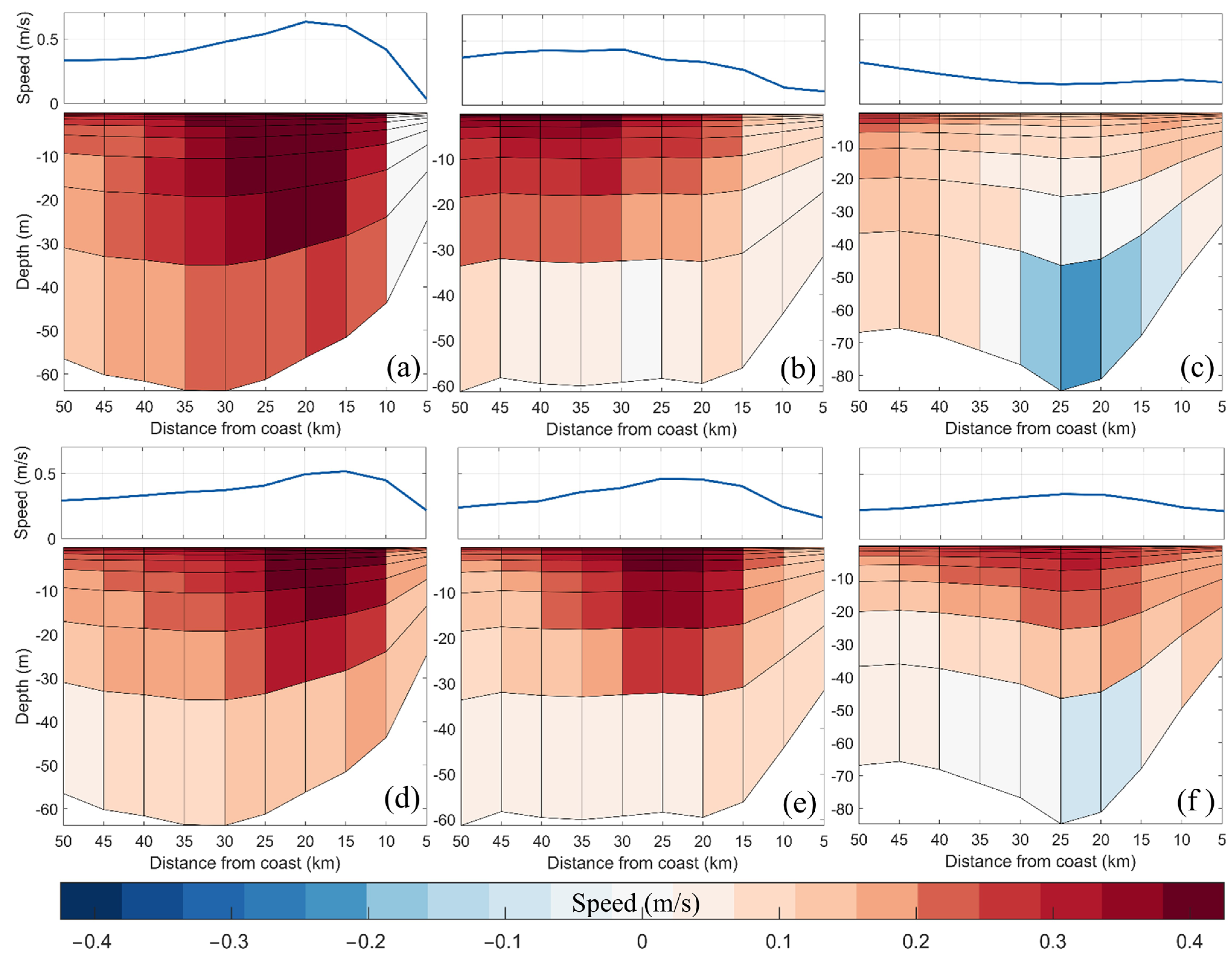
Furthermore, there were three transects designed to present the vertical profile of the model current (Figure 6), and the results are shown in Figure 11. The vertical stratification profile of the ocean current along with transect A indicates that the speeds of the nearshore currents were higher than those of the offshore currents, regardless of whether the tidal forcing was turned on or off (Figure 11a,d). The nearshore currents were more concentrated and closer to the coast with the depth until the water depth reached about 30 m. On the other hand, the flow profiles with tidal forcing were more dispersed than those without tidal forcing, whether in transect A or B. The flow profiles along transect C were generated with two high-velocity peaks when the tidal forcing was turned on in the model (Figure 11c). The locations of the two high-velocity peaks are the same as the branching sites of the probability density distribution in northwestern Taiwan (Figure 9a). Thus, it is possible to infer that these ocean flow branches are caused by the transition between ebb and flood tides.

5. Discussion

In summer, the main ocean current in the TS is a northward flow consisting of the SCS warm current and the Kuroshio branch current [5,6]. These currents flow northward to the southern ECS after passing by northwestern Taiwan. However, there are obvious transitions of ebb and flood tides from the northern TS to the north end of Taiwan twice a day. The flow direction of the ebb current in northern TS is the same as that of the main current in summer, but the flow direction of the flood current is completely opposite. Therefore, there is complicated intra-diurnal variability in currents in northwestern Taiwan. The variability is hard to observe from the long-term average flow field data. However, the average ocean surface current in a six-hour period from CODAR data suggested that there is diurnal tide–current interaction in the northern TS during summer (Figure 3 and Figure 4). We found that the flow direction started to change when the tidal period crossed high and low tides. The flow direction of the nearshore current would change before the offshore current. Moreover, the speed of the nearshore current is higher than that of the offshore current during the flood tide in northern Taiwan, but there was no obvious difference during the ebb period.

In this study, we classified three different flow patterns according to the drifter trajectories that drifted northward through the Penghu Channel. Drifting path 1 is similar to path 2, as both of them are driven northward by the nearshore current, but they separate in northwestern Taiwan (Figure 5). There is an intra-diurnal tide–current interaction caused by the transitions of ebb and flood tides. Therefore, we infer that the difference between these two drifting paths was caused by a tidal effect. To confirm the influence of the tide, we simulated numerous float trajectories in ocean models. The probability density distributions show that drifting paths 1 and 2 occur with tidal forcing (Figure 9a). The distribution of simulated floats that drifted northward is almost the same as that of those that drifted eastward. However, the probability density distribution only shows drifting path 1 in the absence of tidal forcing (Figure 10a). Few floats could drift northward to the ECS when released at the nearshore position. Drifting path 1 appeared when there was no tidal influence in northwestern Taiwan. However, the ocean current flow eastward in northern Taiwan will be hindered by the flood current, forcing the ocean current to flow northward to the ECS (path 2). After the flood period, the ocean current can flow unhindered to northern Taiwan during the ebb period, as the trajectory of path 1. Thus, path 1 and path 2 will alternately appear in the northern TS as the ebb and flood tides’ transition.

The drifting path 1 and path 2 can flow unimpeded by the bottom ridge of CYR after passing through the Penghu Channel, but path 3 is different from them. A previous study simulated the northward near-surface current (at 15 m) in the Penghu Channel in summer, and this current is relatively unimpeded by CYR; only the near-bottom current is deflected anti-cyclonically [19]. In another study, the results of a numerical model showed that the northward current appears to be relatively unimpeded by CYR and bifurcates slightly near the surface (at 20 m) [20]. The results of drifters and simulated floats in this study showed that whether the currents can be deflected by CYR is mainly affected by the distance from the shore. The drifters and floats that pass through the Penghu Channel near the shore will cross over the CYR, whereas those far from the shore are deflected by it. The discrepancy between our results and those of the previous study [19] was caused by the different speeds of the surface current. The surface current speed of that study was up to 1.5 m/s over CYR, so the surface current can be relatively unimpeded by the CYR [19]. However, the flow speeds of simulations in this study were 0.25–0.50 m/s, the same as that of the previous study [20]. Moreover, the drifting speeds of drifters were 0.32–0.68 m/s over CYR (Figure 5), which is also close to our simulation results.

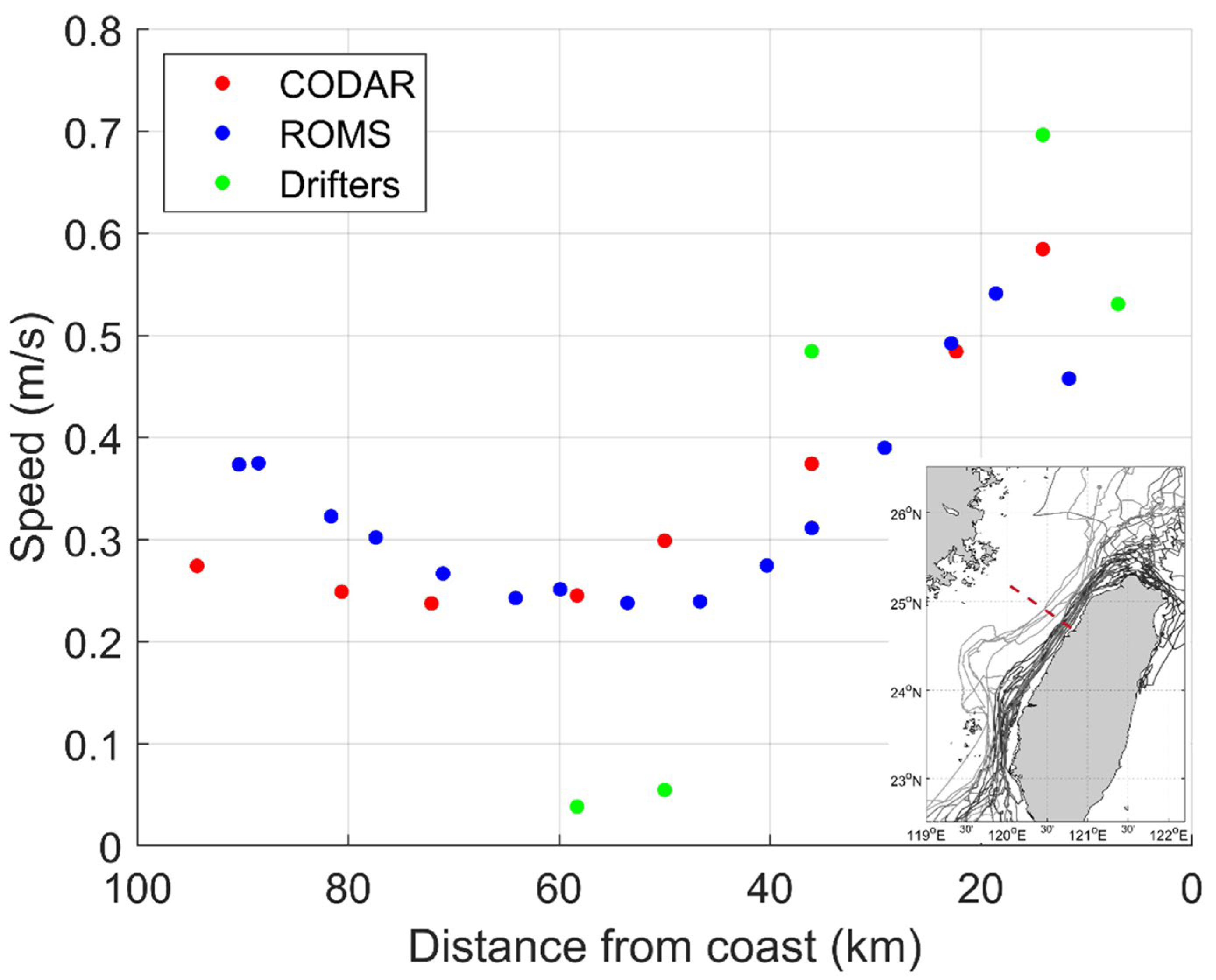
The trajectory of path 3 north of CYR (at 24.5–25°N) is also different from the trajectories of the other two paths. It seems that there are two different current paths. One flows northward along the shore, and the other flows northward at a distance from the shore. Figure 12 shows the average speeds of the cross-shore distribution by the west coast of Taiwan from three datasets, including CODAR, ROMS, and drifters during summer. It should be noted that the average speeds of drifters in Figure 12 were calculated from all drifters passing through the TS in the summer. According to the average velocity of the cross-shore distribution, we found that all three datasets present a rapid alongshore current (Figure 12). It is worth noting that the speed magnitudes of CODAR and ROMS at about 45 km from the coast were reduced to half of those along the coast. Additionally, the velocity magnitude of drifters was even less than 0.10 m/s at a distance of more than 50 km. The results show that there is a significant difference in speed between nearshore and offshore currents. The drifters drifting along path 3 cannot easily blend with those drifting along path 1 and path 2. To sum up, after passing through the Penghu Channel, path 3 is deflected by CYR and flows northward at a distance from the west coast of Taiwan. This geographical factor makes path 3 different from the first two drifting paths, so it flows northward in the middle of the TS to the south of the ECS.

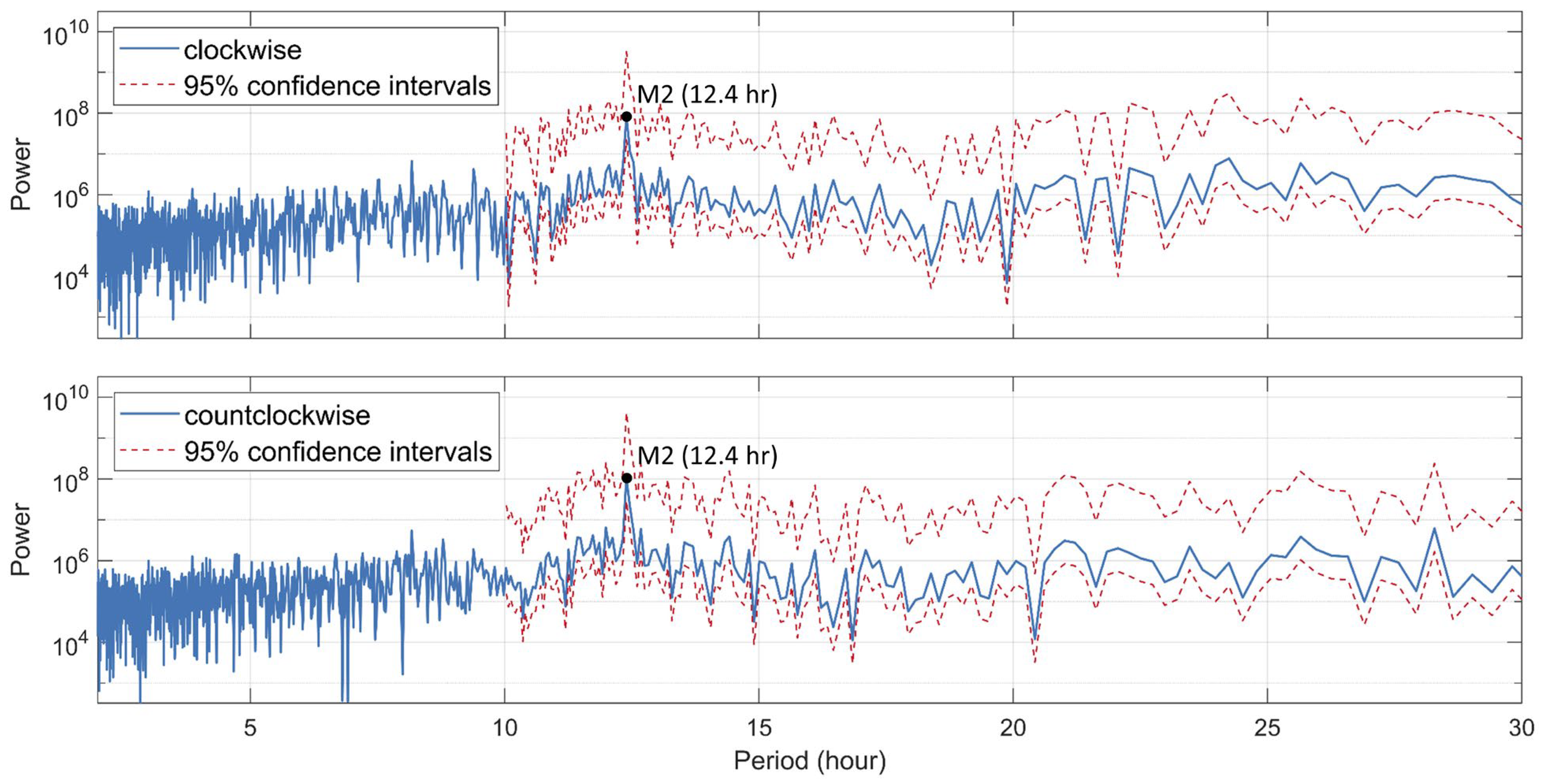
On the other hand, the trajectories of path 2 and path 3 drift northward to the south ECS after passing through the TS. They appear to exhibit a near-inertial oscillation in northeastern Taiwan (Figure 5). According to the inertial oscillation period T_f = π/Ω sin θ, where Ω is the Earth’s rotation rate and θ is latitude, the period is 27.3 h at 26°N. Figure 13 shows the rotary power spectrum of HF radar flow fields in northeastern Taiwan (26°N, 122°E), none of which are close to the inertial oscillation but show a strong semidiurnal tidal period. A previous study also observed that drifter trajectories in the south ECS were oscillated and trapped by strong tidal currents [21]. Therefore, it is speculated that these oscillations were caused by the semidiurnal tide.

6. Conclusions

In this study, we used the HF radar data to find the intra-diurnal tide-current interaction in the north entrance of the TS from average ocean surface currents of six-hour periods in summer. We found that the flow direction of the nearshore current changes before that of the offshore current after high tide and low tide. Moreover, the speed of the nearshore current is faster than that of the offshore current during the flood tide at the north end of Taiwan, but there is no obvious difference during the ebb period.

Due to the tidal effect and complex topography, there are several flow patterns in the TS. To clarify the variations in flow patterns in the TS, we collected 30 satellite tracking drifters that drifted northward through the Penghu Channel. There were 24 drifters among them that could be classified as having one of three types of drifting paths based on their trajectories. Path 1 presents a flow pattern along the west coast of Taiwan from the southwest coast to the northeast coast. Path 2 is the same as path 1 but flows northward to the ECS instead of eastward to the northeast coast of Taiwan. Path 3 presents a flow pattern that moves along the west coast of Taiwan at a distance from the coast after being deflected by the CYR. Each of the drifting paths has a unique trajectory and different drifting speeds.

The difference between paths 1 and 2 is the bifurcation by northwestern Taiwan, where there is a strong tidal effect. From the results of HF radar and several simulations, we confirmed that the factor that causes the difference is the transition between ebb and flood tides. The current flow eastward in northern Taiwan is hindered by flood currents, thereby forcing the current to flow northward to the ECS. The current can flow unhindered to the north side of Taiwan during the ebb tide period. On the other hand, paths 2 and 3 have the same destination with different trajectories in the TS. To find out the reason, we investigated the alongshore velocities of cross-shore distributions from three datasets, including HF radar, satellite drifter, and ocean model datasets. The results of the alongshore velocity show there is a clear difference in speed between nearshore and offshore currents at about 45 km distance from the coast—the speed is reduced to half of that along the coast. This geographical factor makes path 3 different from the first two: it flows northward from the middle side of the TS to the southern part of the ECS after being deflected by CYR.

In conclusion, there are intra-diurnal tide–current interactions in the north entrance of the TS, as observed by HF radar data. Additionally, there are three different flow patterns in the northern TS in summer. This study clarified the causes of these three flow patterns with HF radar data and ocean simulations. The findings will aid in the safety of ship navigation, search and rescue, and tracking of marine debris. However, we do not know the characteristics of the water masses in different currents or even the flow patterns in other seasons. There are still many deficiencies in this study, and more research is needed.

References

- Oey, L.Y.; Chang, Y.L.; Lin, Y.C.; Chang, M.C.; Varlamov, S.; Miyazawa, S. Cross Flows in the Taiwan Strait in winter. J. Phys. Oceanogr. 2014, 44, 801–817. [Google Scholar] [CrossRef]
- Wu, C.R.; Hsin, Y.C. Volume transport through the Taiwan Strait: A numerical study. Terr. Atomos. Oceanic Sci. 2005, 16, 377–391. [Google Scholar] [CrossRef] [Green Version]
- Chen, H.W.; Liu, C.T.; Matsuno, T.; Ichikawa, K.; Fukudome, K.; Yang, Y.; Doong, D.J.; Tsai, W.L. Temporal variations of volume transport through the Taiwan Strait, as identified by three-year measurements. Cont. Shelf Res. 2016, 114, 41–53. [Google Scholar] [CrossRef] [Green Version]
- Hu, J.Y.; Kawamura, H.; Li, C.Y.; Hong, H.S.; Jiang, Y.W. Review on current and seawater volume transport through the Taiwan Strait. J. Oceanogr. 2010, 66, 591–610. [Google Scholar] [CrossRef] [Green Version]
- Chen, D.; Lian, E.; Shu, Y.; Yang, S.; Li, Y.; Li, C.; Liu, P.; Su, N. Origin of the springtime South China Sea warm current in the southwestern Taiwan Strait: Evidence from seawater oxygen isotope. Sci. China Earth Sci. 2020, 63, 1564–1576. [Google Scholar] [CrossRef]
- Guan, B.X.; Fang, G.H. Winter counter-wind currents off the southeastern China coast: A review. J. Oceanogr. 2006, 62, 1–24. [Google Scholar] [CrossRef]
- Tseng, Y.H.; Lu, C.Y.; Zheng, Q.; Ho, C.R. Characteristic analysis of sea surface currents around Taiwan Island from CODAR observations. Remote Sens. 2021, 13, 3025. [Google Scholar] [CrossRef]
- Jan, S.; Chao, S.Y. Seasonal variation of volume transport in the major inflow region of the Taiwan Strait: The Penghu Channel. Deep Sea Res. II Top. Stud. Oceanogr. 2003, 50, 1117–1126. [Google Scholar] [CrossRef]
- Fang, G.; Yang, J.; Zhao, X. A numerical model for the tides and tidal currents in the Taiwan Strait. Acta Oceanol. Sin. 1985, 4, 189–200. [Google Scholar]
- Wang, Y.H.; Jan, S.; Wang, D.P. Transport and tidal current estimates in the Taiwan Strait from shipboard ADCP observations (1999–2001). Est. Coast. Shelf Sci. 2003, 57, 193–199. [Google Scholar] [CrossRef]
- Hsu, P.C.; Lu, C.Y.; Hsu, T.W.; Ho, C.R. Diurnal to Seasonal Variations in Ocean Chlorophyll and Ocean Currents in the North of Taiwan Observed by Geostationary Ocean Color Imager and Coastal Radar. Remote Sens. 2020, 12, 2853. [Google Scholar] [CrossRef]
- Qiu, Y.; Li, L.; Chen, C.T.A.; Guo, X.; Jing, C. Currents in the Taiwan Strait as observed by surface drifters. J. Oceanogr. 2011, 67, 395–404. [Google Scholar] [CrossRef]
- Paduan, J.D.; Rosenfeld, L.K. Remotely sensed surface currents in Monterey Bay from shore-based HF radar (Coastal Ocean Dynamics Application Radar). J. Geophys. Res. Oceans. 1996, 101, 20669–20686. [Google Scholar] [CrossRef]
- Lumpkin, R.; Centurioni, L. Global Drifter Program Quality-Controlled 6-Hour Interpolated Data from Ocean Surface Drifting Buoys; NOAA National Centers for Environmental Information: Washington, DC, USA, 2019.
- Lumpkin, R.; Maximenko, N.; Pazos, M. Evaluating where and why drifters die. J. Atmos. Oceanic Technol. 2012, 29, 300–308. [Google Scholar] [CrossRef]
- Yang, D.; Yin, B.; Liu, Z.; Bai, T.; Qi, J.; Chen, H. Numerical study on the pattern and origins of Kuroshio branches in the bottom water of southern East China Sea in summer. J. Geophys. Res. Oceans 2012, 117. [Google Scholar] [CrossRef]
- Liu, X.; Wang, D.P.; Su, J.; Chen, D.; Lian, T.; Dong, C.; Liu, T. On the vorticity balance over steep slopes: Kuroshio intrusions northeast of Taiwan. J. Phys. Oceanogr. 2020, 50, 2089–2104. [Google Scholar] [CrossRef]
- Egbert, G.D.; Erofeeva, S.Y. Efficient inverse modeling of barotropic ocean tides. J. Atmos. Ocean. Technol. 2002, 19, 183–204. [Google Scholar] [CrossRef] [Green Version]
- Jan, S.; Wang, J.; Chern, C.S.; Chao, S.Y. Seasonal variation of the circulation in the Taiwan Strait. J. Mar. Syst. 2002, 35, 249–268. [Google Scholar] [CrossRef]
- Wu, C.R.; Chao, S.Y.; Hsu, C. Transient, seasonal and interannual variability of the Taiwan Strait current. J. Oceanogr. 2007, 63, 821–833. [Google Scholar] [CrossRef]
- Hsu, P.C.; Centurioni, L.; Shao, H.J.; Zheng, Q.; Lu, C.Y.; Hsu, T.W.; Tseng, R.S. Surface Current Variations and Oceanic Fronts in the Southern East China Sea: Drifter Experiments, Coastal Radar Applications, and Satellite Observations. J. Geophys. Res. Oceans 2021, 126, e2021JC017373. [Google Scholar] [CrossRef]
Figure 1.
Topography around the TS.
Figure 2.
The average flow field in the summer of 2017 obtained from HF radar data. The red squares are the positions of CODAR stations around Taiwan.
Figure 3.
Average flow fields of six-hour periods (a) after high tide, (b) from one hour after high tide, (c) from two hours after high tide, (d) from three hours after high tide, (e) from four hours after high tide, and (f) from five hours after high tide in the summer of 2017. The green square is the tidal station (Linshanbi, located at 25.2839°N, 121.5103°E). The blue arrows represent the averages of flow directions north of Taiwan.
Figure 4.
Average flow fields of six-hour periods (a) after low tide, (b) from one hour after low tide, (c) from two hours after low tide, (d) from three hours after low tide, (e) from four hours after low tide, and (f) from five hours after low tide in the summer of 2017. The green square is the tidal station (Linshanbi, located at 25.2839°N, 121.5103°E). The blue arrows represent the averages of flow directions north of Taiwan.
Figure 6.
Wind field and seabed terrain set in ROMS model. The red points represent the starting points of the simulated floats. Point N means nearshore and point O means offshore. The green points represent the transects of the vertical profile of ocean flow.
Figure 7.
Average surface flow fields of the ROMS simulation in summer.
Figure 8.
Comparisons of average flow fields between ROMS and CODAR data. The dots represent the mean and the bars represent the standard deviation of each latitude band.
Figure 9.
Probability density distribution of simulated floating trajectories released from (a) nearshore and (b) offshore points in the ROMS simulation with tidal forcing turned on.
Figure 10.
Probability density distributions of simulated trajectories of floats deployed from (a) nearshore and (b) offshore points without tidal forcing.
Figure 11.
Vertical stratification profile of ocean current along transect A (a,d), along transect B (b,e), and along transect C (c,f) simulated using the ROMS model with (a–c) or without (d–f) tidal forcing. The solid blue line represents the surface speed of each vertical profile. Red (Blue) shading represents the direction toward the inside (outside) the plane of the paper (or screen).
Figure 12.
Average alongshore speeds of the cross-shore distributions from three datasets during summer. The red dotted line represents the transect for the cross-shore distribution.
Figure 13.
Rotary power spectrum of HF radar in northern Taiwan (26°N, 122°E).
Publisher’s Note: MDPI stays neutral with regard to jurisdictional claims in published maps and institutional affiliations. |
© 2022 by the authors. Licensee MDPI, Basel, Switzerland. This article is an open access article distributed under the terms and conditions of the Creative Commons Attribution (CC BY) license (https://creativecommons.org/licenses/by/4.0/).
Share and Cite
MDPI and ACS Style
Lu, C.-Y.; Hsu, P.-C.; Zheng, Q.; Ho, C.-R. Variations in Flow Patterns in the Northern Taiwan Strait Observed by Satellite-Tracked Drifters. Remote Sens. 2022, 14, 2154. https://doi.org/10.3390/rs14092154
AMA Style
Lu C-Y, Hsu P-C, Zheng Q, Ho C-R. Variations in Flow Patterns in the Northern Taiwan Strait Observed by Satellite-Tracked Drifters. Remote Sensing. 2022; 14(9):2154. https://doi.org/10.3390/rs14092154
Chicago/Turabian StyleLu, Ching-Yuan, Po-Chun Hsu, Quanan Zheng, and Chung-Ru Ho. 2022. "Variations in Flow Patterns in the Northern Taiwan Strait Observed by Satellite-Tracked Drifters" Remote Sensing 14, no. 9: 2154. https://doi.org/10.3390/rs14092154
Note that from the first issue of 2016, this journal uses article numbers instead of page numbers. See further details here.