
Generation and Optimization of Spectral Cluster Maps to Enable Data Fusion of CaSSIS and CRISM Datasets
by
 and
and
Michael Fernandes
1, 
Alexander Pletl
1,
Nicolas Thomas
2,*,
Angelo Pio Rossi
3 and
Benedikt Elser
1 1
Technologie Campus Grafenau, Technische Hochschule Deggendorf, 94481 Grafenau, Germany
2
Physikalisches Institut, University of Bern, 3012 Bern, Switzerland
3
Department of Physics and Earth Sciences, Jacobs University Bremen, 28759 Bremen, Germany
*
Author to whom correspondence should be addressed.
Remote Sens. 2022, 14(11), 2524; https://doi.org/10.3390/rs14112524
Submission received: 8 April 2022
/
Revised: 17 May 2022
/
Accepted: 19 May 2022
/
Published: 25 May 2022
(This article belongs to the Special Issue Planetary Exploration Using Remote Sensing)
Abstract
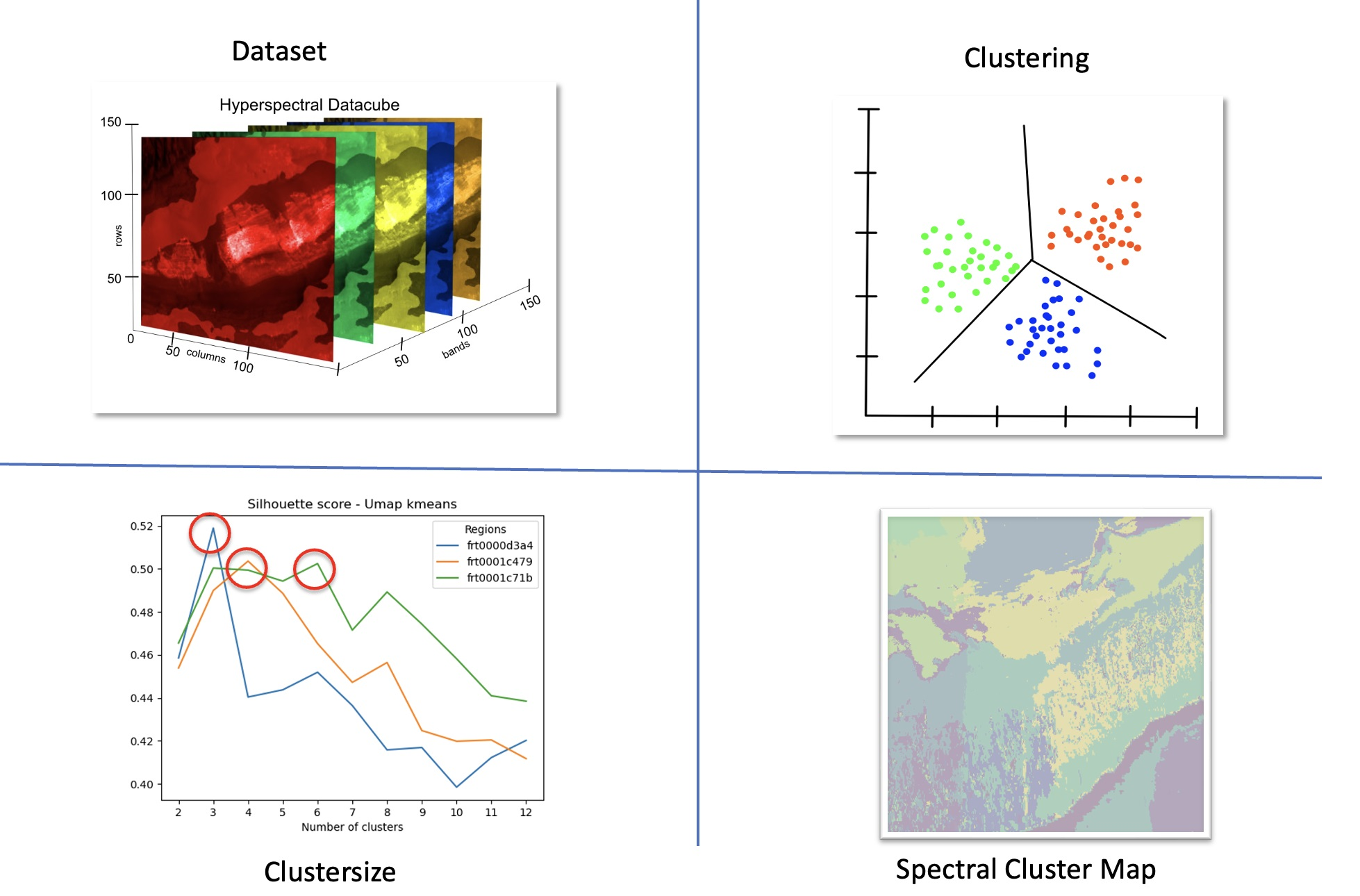
:Four-band color imaging of the Martian surface using the Color and Stereo Surface Imaging System (CaSSIS) onboard the European Space Agency’s ExoMars Trace Gas Orbiter exhibits a high color diversity in specific regions. Not only is the correlation of color diversity maps with local morphological properties desirable, but mineralogical interpretation of the observations is also of great interest. The relatively high spatial resolution of CaSSIS data mitigates its low spectral resolution. In this paper, we combine the broad-band imaging of the surface of Mars, acquired by CaSSIS with hyperspectral data from the Compact Reconnaissance Imaging Spectrometer (CRISM) onboard NASA’s Mars Reconnaissance Orbiter to achieve a fusion of both datasets. We achieve this using dimensionality reduction and data clustering of the high dimensional datasets from CRISM. In the presented research, CRISM data from the Coprates Chasma region of Mars are tested with different machine learning methods and compared for robustness. With the help of a suitable metric, the best method is selected and, in a further step, an optimal cluster number is determined. To validate the methods, the so-called “summary products” derived from the hyperspectral data are used to correlate each cluster with its mineralogical properties. We restrict the analysis to the visible range in order to match the generated clusters to the CaSSIS band information in the range of 436–1100 nm. In the machine learning community, the so-called UMAP method for dimensionality reduction has recently gained attention because of its speed compared to the already established t-SNE. The results of this analysis also show that this method in combination with the simple K-Means outperforms comparable methods in its efficiency and speed. The cluster size obtained is between three and six clusters. Correlating the spectral cluster maps with the given summary products from CRISM shows that four bands, and especially the NIR bands and VIS albedo, are sufficient to discriminate most of these clusters. This demonstrates that features in the four-band CaSSIS images can provide robust mineralogical information, despite the limited spectral information using semi-automatic processing.

1. Introduction
One of the major difficulties in the investigation of our solar system is that high resolution datasets returned by in situ orbiting spacecraft are usually incomplete, either spatially, spectrally or both. Observations of the surface of Mars have shown that high-resolution remote sensing is needed to establish the physico-chemical properties of specific areas. Only then can interpretation of the processes involved follow and other aspects, such as the suitability for a future landing, be considered. High resolution, however, implies high data volume with reduced surface coverage. Instruments such as the High Resolution Imaging Science Experiment (HiRISE) [1] and Compact Reconnaissance Imaging Spectrometer (CRISM) [2] onboard NASA’s Mars Reconnaissance Orbiter (MRO) and CaSSIS [3] onboard the European Space Agency’s (ESA) ExoMars Trace Gas Orbiter (TGO) are good illustrations of the problem. All three instruments have high resolution, their data in total amounts to less than 5% surface coverage of the planet. Nonetheless, the respective datasets are large suggesting that automated processing techniques can produce significant benefits. This has led us to pose the question of whether imaging spectrometer datasets from CRISM can be linked to broad-band imaging datasets from CaSSIS to improve interpretation through both spatial interpolation of the spectra and extrapolation by taking advantage of redundancy in the spectral domain.
Spectral data are complex because of resolution issues and the high number of bands and subclasses. Therefore, our paper relies on unsupervised classification, which is an important standard procedure in geospatial analysis [4], especially when analyzing hyperspectral data with insufficient calibration in-field data. For analysis purposes, the combination of band information and spatial distributions is formed into a data structure—in this paper called Spectral Cluster Maps (SCMs). High dimensional data are transferred to a low latent variable representation by directly applying advanced methods on the full spectrum itself, and these clusters can be related to the underlying geochemical composition (compare Gao et al. [5]). Therefore, it is essential to find suitable unsupervised dimensionality reduction techniques to produce accurate SCMs before applying various clustering algorithms on the feature space. The principal component analysis (PCA) [6] is the most commonly used technique applied to spectral data (e.g., [7,8]) and we use this here to benchmark against more elaborate algorithms. In recent studies of Machine Learning Networks, approaches such as t-SNE [9] have achieved promising results. Distinct grouping has been obtained by focusing on more local structures and mapping the feature space into a low dimensional representation. Compare among others the works of Pouyet et al. and Song et al. [10,11] or the self-organizing maps technique (SOM) developed by Kohonen [12], which has already been proposed for generating spectral databases. Specifically for Mars, a recent study published by Gao et al. [5] proposes the autoencoder technique for spectral application. The application of the UMAP technique to spectral data is relatively rare at present. Groups tackling this issue include Picollo et al. [13] and Wander et al. [14]. The most relevant work in this context is the recently published paper by D’Amore and Padovan [15] using UMAP for mapping reflectance spectra from Mercury. Publications using UMAP are more abundant in the biology research field [16,17]; however, due to its speed and robustness, its wider application for planetary science is desirable.
Generating Spectral cluster maps from CRISM and Cassis data has a direct impact on geologic mapping activities (e.g., [18]). The planetary geologic mapping process itself relies on basic geometric and stratigraphic principles, historically limited by the availability of image and topographic data. The availability of compositional data in recent decades allowed the inclusion of different kind of methods, varying from heuristical methods to statistical approaches [19,20,21,22].
To assess the feasibility and efficacy of our approach, we have selected Coprates Chasma, as the region exhibits significant mineralogical (color) diversity in CRISM and CaSSIS observations.
The rest of this paper is structured as follows: Section 2 describes the data and the preprocessing used. The examined dimensionality reduction techniques and clustering algorithms used in this study are also briefly presented. In Section 3, the obtained results are illustrated and discussed. Section 4 proceeds with a geological mapping based on the image products and links to the CaSSIS data. The paper finishes with a brief conclusion (Section 5).
2. Materials and Methods
This section is devoted to the machine learning techniques considered in this study. The data and their origin are also described.
2.1. Data Source
CRISM is a high spectral resolution visible and infrared mapping spectrometer currently in orbit around Mars onboard NASA’s Mars Reconnaissance Orbiter (MRO) [2]. For this analysis, hyperspectral datasets (compare Appendix B for a list) provided by John Hopkins University through the Planetary Data System hosted at Washington University St. Louis [23] were selected.
CRISM provides 2D spatially resolved spectra over a wavelength range of 362 nm to 3920 nm at 6.55 nm/channel. The spatial resolution is typically around 18 m/px. Pelkey et al. [24] and Viviano et al. [25] generated a feature set of “image products” from CRISM spectra, which are strongly related to the geochemical composition of the Martian surface.
The CaSSIS instrument is a high spatial resolution color and stereo imager [3] currently in orbit around Mars onboard the European Space Agency’s ExoMars Trace Gas Orbiter (TGO). CaSSIS returns images at 4.5 m/px from the nominal 400 km altitude orbit in four colors using a push-frame technique. The images typically sample an area of approximately 9 km × 40 km on the Martian surface with around 24 images per day being acquired. The filters were selected to provide good mineral diagnostics in the visible wavelength range (400–1100 nm) and to complement the filters in the extremely high-resolution HiRISE system onboard NASA’s Mars Reconnaissance Orbiter (MRO).
Studies by Tornabene et al. [26] illustrated the potential for mineralogical diagnostics using preflight calibration data. Good performance in flight has also been established. Parkes Bowen et al. [27,28] have demonstrated the effectiveness of CaSSIS through identification of two spectrally and morphologically distinct subunits of the Oxia Planum (the ExoMars rover landing site) clay unit—one indicative of Fe/Mg-rich clay minerals and one showing decametre scale fracturing with Fe/Mg-rich clay mineral/olivine signatures.
2.2. Data and Location
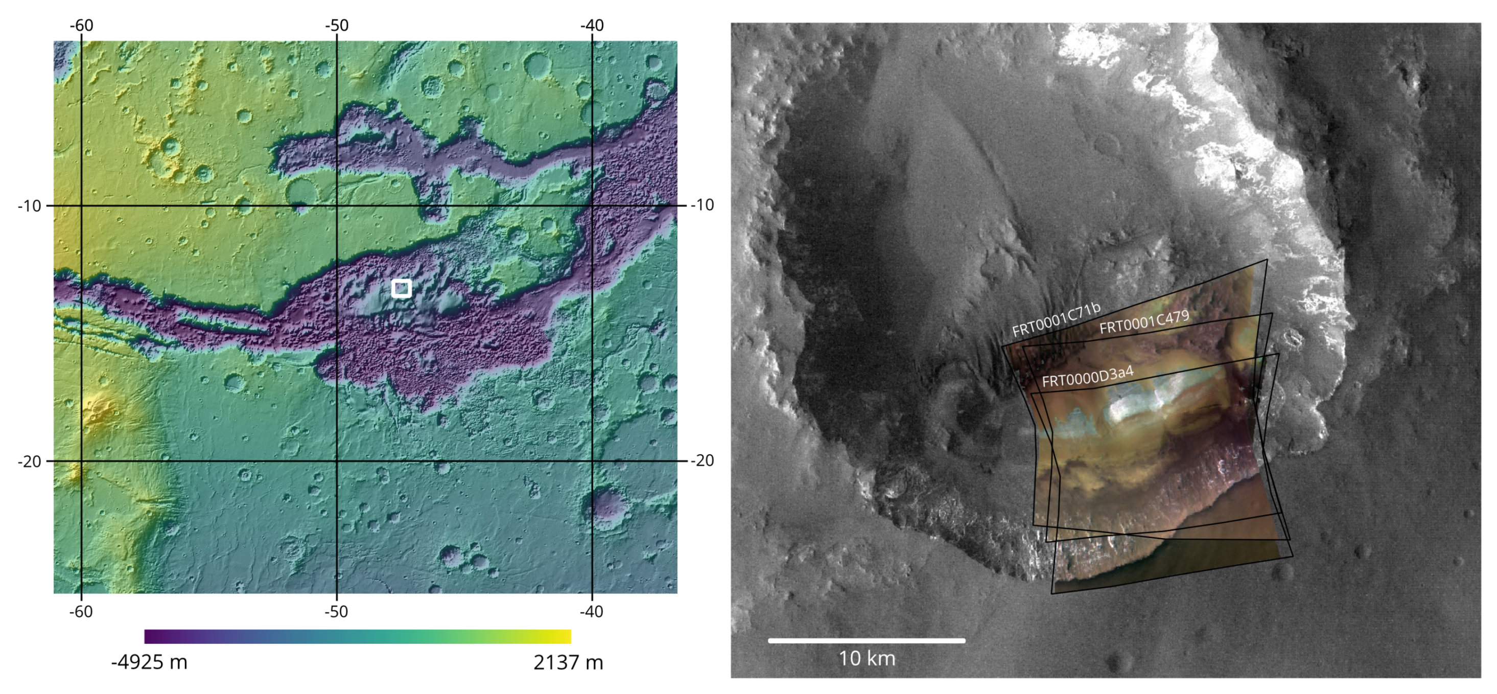
Coprates Chasma, a central part of Valles Marineris tectonic system on Mars, was selected for initial studies. Coprates Chasma is a 1000 km long, 100 km wide linear trough connecting Melas Chasma (central Valles Marineris) to Capri Chasma (eastern Valles Marineris). The CRISM data files used for this study were the MTRDR products FRT0000d3a4, FRT0001c479 and FRT0001c71b (compare Figure 1).
The area exhibits significant color diversity at visible wavelengths and is of major interest in studies of the history of liquid water on Mars. Geologic features, including fluvial topography (e.g., [31,32]) and the distribution of a variety of aqueous minerals including sulfates, are evidence of the influence of water in Valles Marineris [33].
Weitz and Bishop [34] investigated the morphology, mineralogy and stratigraphy of light-toned layered deposits in the same region and found numerous hydrated minerals, including Al-phyllosilicates, Fe/Mg-phyllosilicates, hydrated silica, hydrated sulfates, jarosite and acid alteration products based on visible to near-IR spectral analysis (e.g., [35]). They suggest that valleys sourced from water along the plateau may have flowed downward into one or more troughs with changing aqueous chemistry resulting in the diverse mineralogies.
Fueten et al. [36] investigated layered deposits in northern Coprates Chasma. Here, hydrated sulfates have been detected indicating alteration or deposition by liquid water. There is also evidence of pedogenesis (weathering of basaltic soils by continuous exposure to water percolating down from the surface), which can result in layers of aluminium phyllosilicates forming over layers of iron-magnesium phyllosilicates [37] on the plateau around Coprates Chasma [38]. The primary test area is centred on an exposure of lighter-toned material within a 25 km diameter crater. It was expected to give clear mineralogically diverse signals in CRISM and CaSSIS data.
2.3. Preprocessing
Our preprocessing steps are similar to the steps in Gao et al. [5]: we select a subimage with a size of 400 × 400 pixels from the image area in order to exclude unwanted empty areas from the calculation. Like Gao et al. [5] we also perform a per pixel normalization by removing values outside 0 and 1. To cover the range of the CaSSIS instrument, we restrict data to a wavelength range of 436–1106 nm and adjust the preprocessing accordingly. This range corresponds to 88 channels of the CRISM hyperspectral dataset. In summary, we have (400 × 400) × 88 vectorized images.
2.4. Dimensionality Reduction Techniques
We compared several techniques for dimensionality reduction and feature extraction. Dimensionality reduction is needed to reduce the high data volume into a feature space with lower dimension while keeping the relevant information.
We introduce each technique briefly.
- Autoencoder
Generally speaking, an autoencoder is an unsupervised feature extraction procedure based on a neural network. It consists of three main components: an encoder network, a latent feature representation and a decoder network. The concept of the encoder is to re-compile the data such that the main information of the input is represented by a certain number of latent variables. The dimensionality of the reduced feature space is a user-chosen positive number.
The aim of the decoder is to rescale the encoder output to the initial shape of the data, as described by Kovenko et al. [39]. The model is trained by using back-propagation. More information on this topic can be found in [40].
To measure the accuracy during the training process, a loss function is employed, which has to be minimized. For an autoencoder, it is common practice to use the well-known mean squared error or mean absolute error to evaluate performance. In this paper, we adopt the approach of Gao et al. [5] and insert the spectral angle (SA) as a loss function. This is denoted by:
where x is the input data and is the reconstructed dataset. As pointed out by Gao et al. [5] this maintains the capability of capturing small features in the spectra.
- t-SNE
The t-distributed Stochastic Neighbor Embedding (t-SNE) technique, introduced by van der Maaten and Hinton in 2008 [41], is a pioneering approach for cutting down multidimensional data. Because of its remarkable ability to scale high-dimensional data to lower dimensions, acceptance and adoption is rising in the machine learning community [9]. The idea is to express the similarities between two points and as conditional probabilities by converting the Euclidean distances:
where is the variance of the Gaussian distribution that is centered on data point . For the lower-dimensional representation, a similar conditional probability is likewise calculated for and assigning to the high-dimensional data points and :
In order to avoid overcrowding, a Student t-distribution with one degree of freedom is used here to model the probabilities. The projections, and , have to be mapped in the way that they correctly rebuild the similarities between the high-dimensional data points, implying that the conditional probabilities and are equal.
Similar to the autoencoder, an iterative algorithm is exploited to minimize a cost function denoted by the Kullback–Leibler divergence [42]. An input parameter to the t-SNE algorithm is the perplexity, which can be construed as a smoothness measure of the effective number of neighbors.
- UMAP
In 2018, McInnes and Healy [43] presented the Uniform Manifold Approximation and Projection (UMAP) as a method for dimensionality reduction and data visualization. The idea and computation resembles the one for t-SNE to a large extent. A concise overview of the algorithm is given by Allaoui et al. [44]. UMAP aims to represent the dataset in a fuzzy topological structure. In order to build such a structure, the data points are represented in a high-dimensional weighted graph. Each edge weight depicts the probability that two points are connected and is defined by:
where depicts the distance between the i-th and j-th data points and is the distance between i-th data points and its first nearest neighbor.
Analogous to t-SNE, a lower-dimensional representation has to be determined which properly reproduces the relations of the data points in the high dimensional graph. To model these low dimensional similarities, UMAP uses a distribution similar to the Student t-distribution:
In the default UMAP implementation, and are used but setting and results in the Student t-distribution applied in t-SNE [43].
For optimization the low-dimensional representation UMAP uses binary cross-entropy as a cost function. It is also necessary to specify the number of nearest neighbors. As outlined by Vermeulen et al. [45], this parameter controls how UMAP handles local versus global structure in the data. A small value affects concentration on very local structure, while a larger value provokes UMAP to search for larger neighborhoods.
For benchmarking the proposed techniques, we implement the standard statistical principal component analysis (PCA) in our data pipeline.
2.5. Clustering Algorithms
In our analysis, we use well-known and established procedures for clustering the data. The K-Means clustering algorithm was published 1967 by MacQueen [46]. Starting by initializing a set of k cluster centers, K-Means aims to minimize the Euclidean Distance between all data points x and their corresponding cluster centers of the cluster set C.
The Gaussian Mixture model (GMM) inserts Gaussian distributions and evaluates cluster membership based on likelihoods rather than distances [47]. The cluster centers are the means of the distributions.
To overcome the potential issue of uncertainty in the clustering assignment, the Fuzzy-c-Means clustering algorithm can be applied. Each data point can be assigned to several clusters by allocating probabilities with which it belongs to each cluster [48].
The Self-Organizing Maps (SOM) technique developed by Teuvo Kohonen [12,49] is another neural network based approach which projects high dimensional datasets into a low-dimensional representation, inspired by the different neurological sensory mapping in the cortex of the brain. This mapping can be achieved by different kinds of “self-organized” unsupervised learning techniques.
3. Results
3.1. Experiment
In the previous section, various dimensionality reduction techniques and clustering algorithms were introduced. To evaluate each approach in its ability to generate well-clustered SCMs, the experiment was designed as follows: using three different preprocessed CRISM datasets (FRT0000d3a4, FRT0001c479 and FRT0001c71b), we examine each method for its clustering property. A method was defined by the combination of the discussed dimensionality reduction techniques and clustering algorithms. In total, a set of 16 different methods were studied.
For the autoencoder, we follow Gao et al. [5] and determine the number of latent variables by HySime [50]. As an activation function, a rectified linear unit (ReLU) was used. To project the data to a lower dimensional space we continued to use PCA with five extracted components, since this number of components explain about 95% of the variance in the data. In the case of t-SNE and UMAP, the original spectral dimension was reduced to two-dimensional data. The perplexity and neighbors parameter, respectively, used for the manifold approximation was set to 100. The clustering was performed by using the standard implementations of all algorithms [51,52,53]. As the true number of classes is not known, the number of clusters under investigation ranged from 2 to 20 clusters.
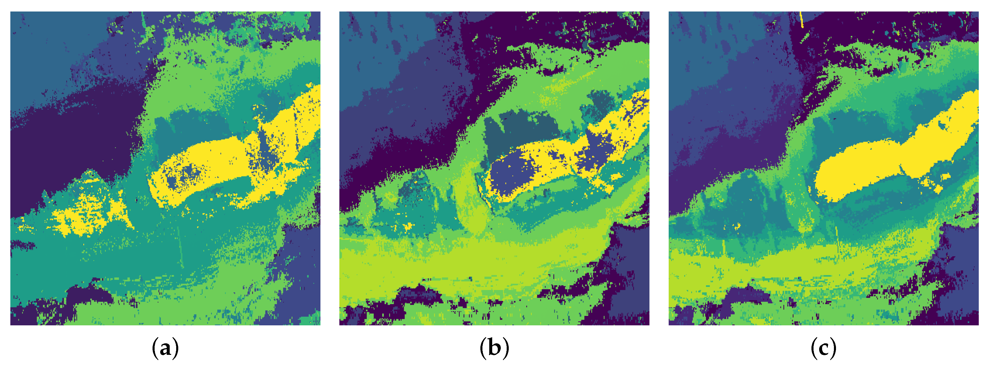
To have a better idea of the shape of the obtained results, Figure 2 shows a subset of the generated SCMs. Each image features a different investigated method for a number of 10 clusters, based on the FRT0001c71b dataset. Cluster membership is characterized by color in the pictures. We illustrated the results of an autoencoder in Figure 2a as comparison to the method established by Gao [5]. Figure 2b shows the results using the standard PCA method, while Figure 2c shows our result using UMAP. Analysis of mineralogy will be later be discussed in our analysis of image browse products.
The structure of the individually produced cluster maps does not differ fundamentally. In particular Figure 2a,c exhibit very similar clustering properties. However, there are differences in the details, indicating that some algorithm combinations are better than others.
3.2. Evaluation
To assess the clustering performance in a quantitative manner, we compute multiple unsupervised cluster-separation metrics for evaluation. To start with, the Calinski–Harabasz (CH) index [54] for a dataset E with pixels and split into k clusters is defined as the ratio of the dispersion between and within clusters:
where:
with denoting the set of points in cluster q, the center of cluster q, the center of E and the number of points in cluster q. The measure indicates a higher score when clusters are dense and well separated.
The Davies–Bouldin (DB) index [55] is based on the average similarity between each cluster i and its most similar one j and is given by:
where:
is the cluster similarity measure, is the cluster diameter and is the distance between cluster centroids i and j. A lower score refers to a higher cluster validity.
As a final measure, the Silhouette Coefficient is bounded between −1 for incorrect clustering and +1 for highly dense clustering whereby scores around zero portend to overlapping clusters. Thus, a significant advantage of this metric is that it allows direct conclusions about the goodness of the clustering algorithm. The Silhouette Coefficient (SC) [56] for a single sample can be written as:
The measure is the ratio of the mean distance a between a point and all other points in the same group and the mean distance b between the point and all samples in the next nearest cluster. The value of SC for a produced SCM is the average of the coefficient for each pixel.
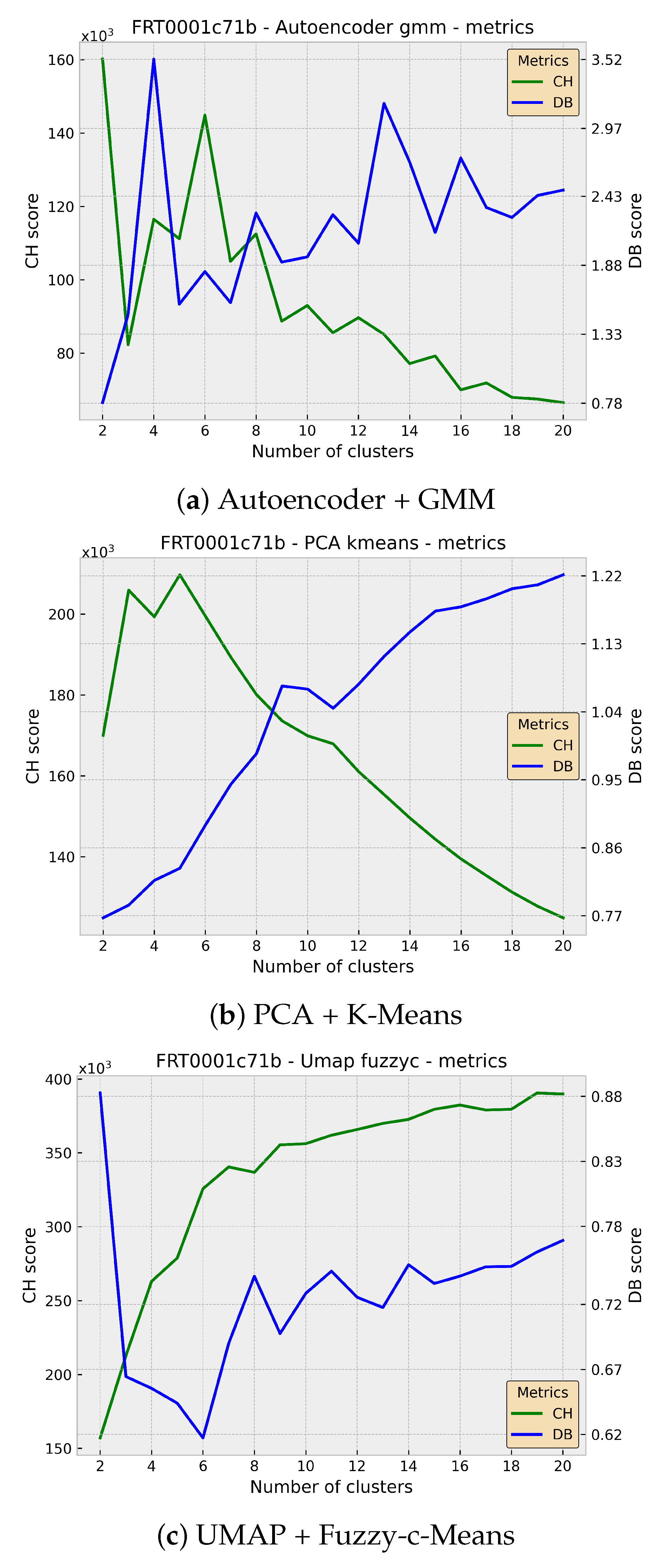
In order to identify the most appropriate method, the metrics are reported over all the calculated number of clusters. The first two measures (CH, DB) are fast to compute and will be shown as a baseline. Figure 3 illustrates the values of the scores plotted against the number of clusters for the same dataset and methods as the pictured SCMs in Figure 2. Some of the graphs show strong fluctuations. However, there exists a high level of evidence for a rather small number of clusters according to the reported scores (compare Figure 4).
Therefore, we proceed with a further analysis in which the mean of the measures over a predefined number of clusters is calculated. As pointed out, there is a strong trend for a small number of classes. Thus, the examination was restricted to a class range of 3 to 7.
In Table 1, we list the mean values of the CH score for all three CRISM selected spectral cubes and all methods. As outlined by Milligan and Cooper [57], the CH score is a powerful criterion for evaluating the validity of clustering (compare Appendix A for the DB index). Apart from a few exceptions, there is a consistent pattern between the Calinski–Harabasz and Davies–Bouldin metric when establishing rank statistics of the individual scores for each dataset where a higher rank invokes denser clusters.
On first viewing, some general remarks can be made. The most striking one is that the UMAP in combination with any examined clustering algorithm performs best across all three spectral images in terms of the CH score whereas the Autoencoder + GMM displays the lowest score in two of three cases. Broken down by dimensionality reduction technique, there is no clear ranking after UMAP. However, the results suggest that the t-SNE approach is also capable of outperforming the Autoencoder and PCA in the case of the FRT0000d3a4 and FRT0001c479 data.
Another finding is that K-Means and Fuzzy-c-Means have higher scores in comparison with the other clustering algorithms for the same feature extraction approach. However, this statement should be treated with caution, since both the CH and the DB index tend to higher and lower scores, respectively, for convex clusters like those generated by K-means and Fuzzy-c-Means.
Nevertheless, UMAP + K-Means can be identified as the best method in our experimental setting.
Additionally, we tracked the computation time for each dimensionality reduction technique. On average, PCA is the fastest technique with 4 s CPU time, while the duration for the t-SNE is much longer (1675 s). The Autoencoder (559 s) and UMAP (789 s) rank in the middle field. (Processor: Intel Xeon Gold 6140, 2.3 GHz, 8 virtual CPUs).
After the evaluation and selection of the best method to create SCMs from our Mars data, we need to determine the most appropriate number of clusters. For this purpose, we take the Silhouette coefficient as a validation measure as it also enables us to make some remarks about the goodness of the clusters in general. In Figure 4, the metric is reported for the UMAP + K-Means method over a reduced range of possible clusters.
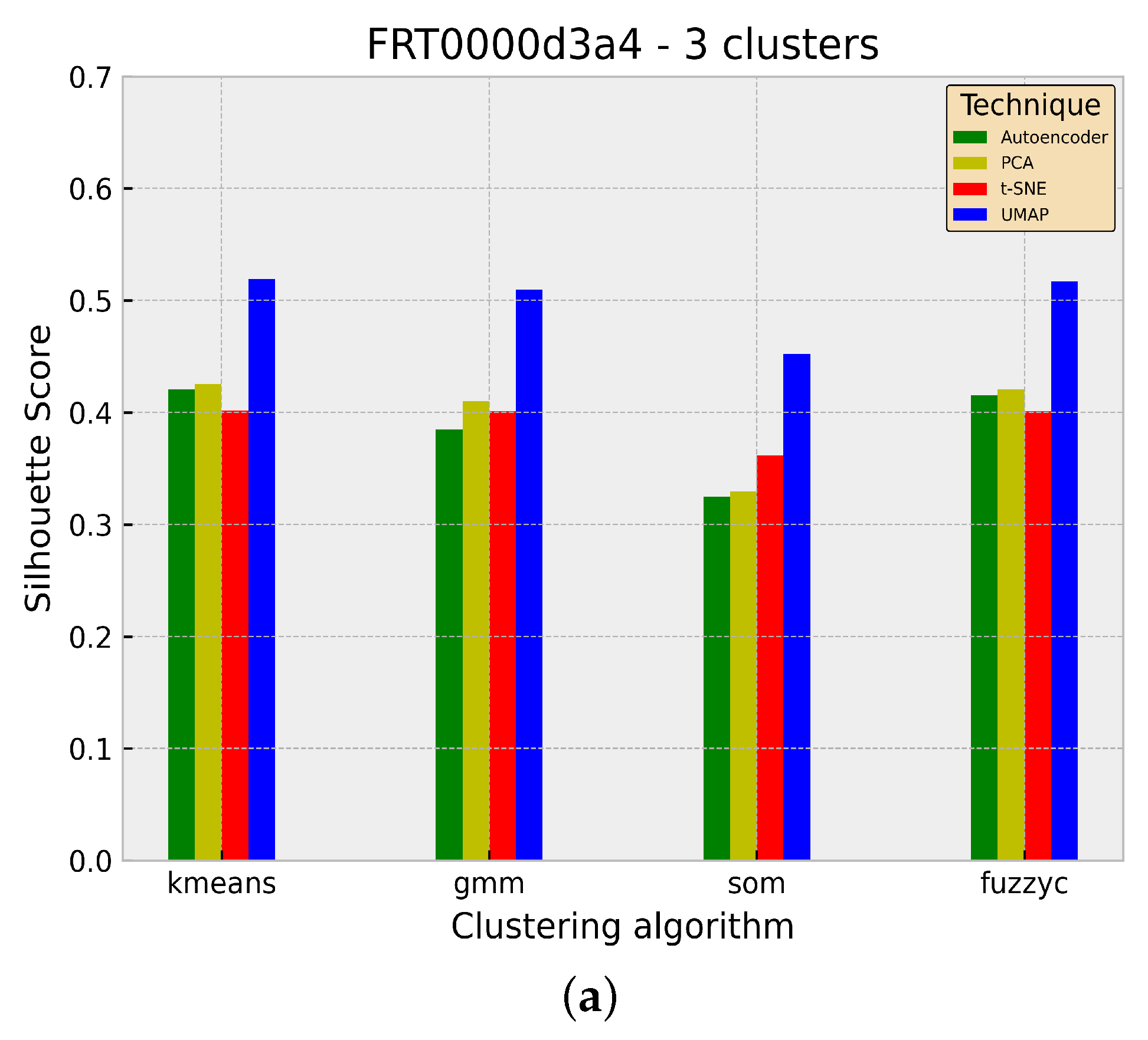
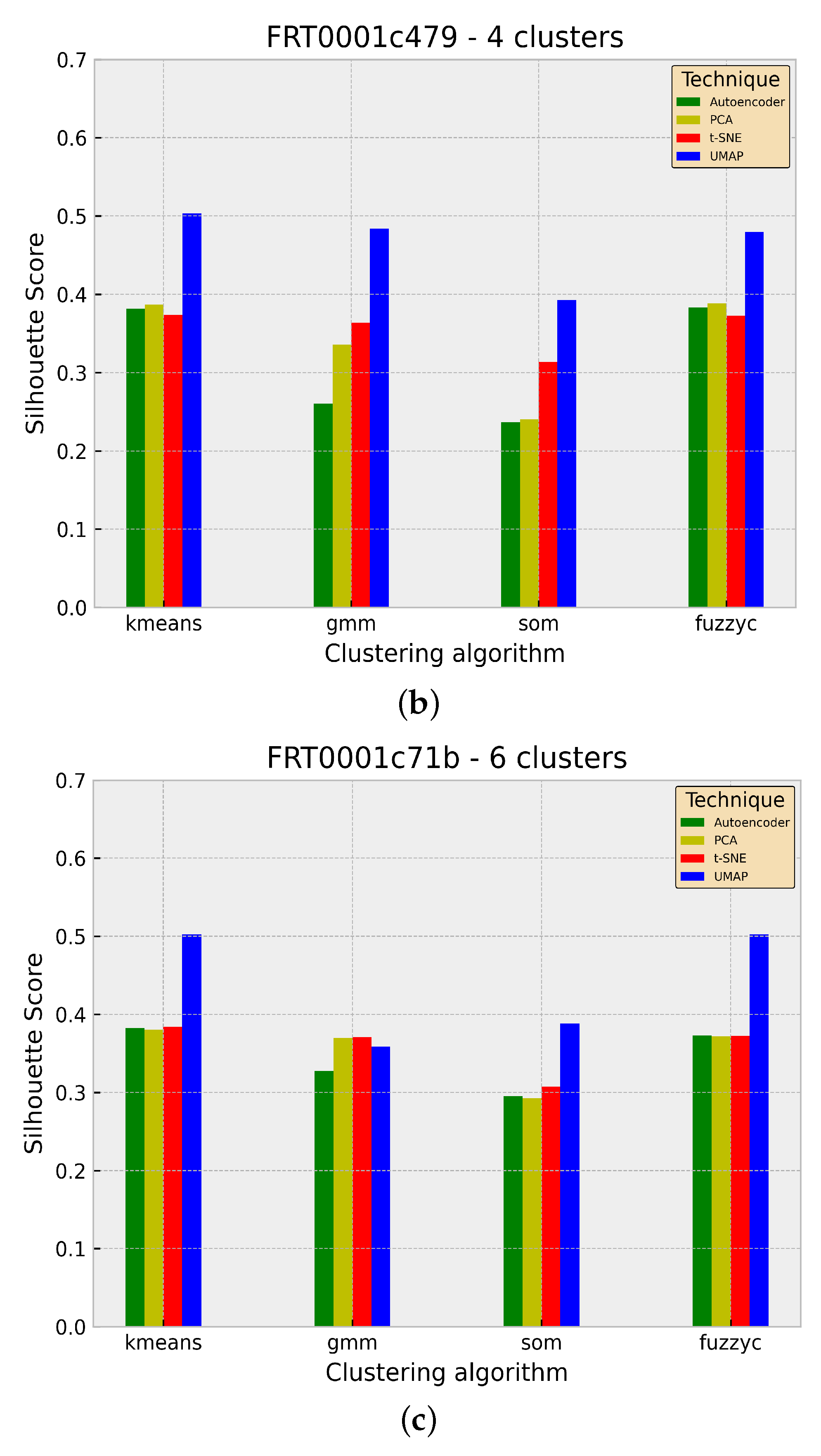
In general, all graphs confirm the choice of a small number of classes as the values for the coefficient drop with an increasing number of clusters. The corresponding number of clusters to the spotted maximum score for each region is as follows: three clusters for FRT0000d3a4, four clusters for FRT0001c479 and six clusters for FRT0001c71b. These findings are mostly in line with the CH and DB index. Furthermore, all maximum scores are about 0.50, and hence, indicate an accurate clustering in large parts of the array.
To demonstrate the superior performance of the UMAP dimensionality reduction technique in the context of Mars data and particularly of the UMAP + K-Means approach compared with the remaining methods, Figure 5 shows the Silhouette coefficient for the identified number of clusters. While the Autoencoder, PCA and t-SNE show similar values across the four clustering algorithms, the UMAP exhibits significantly higher scores.
4. Discussion
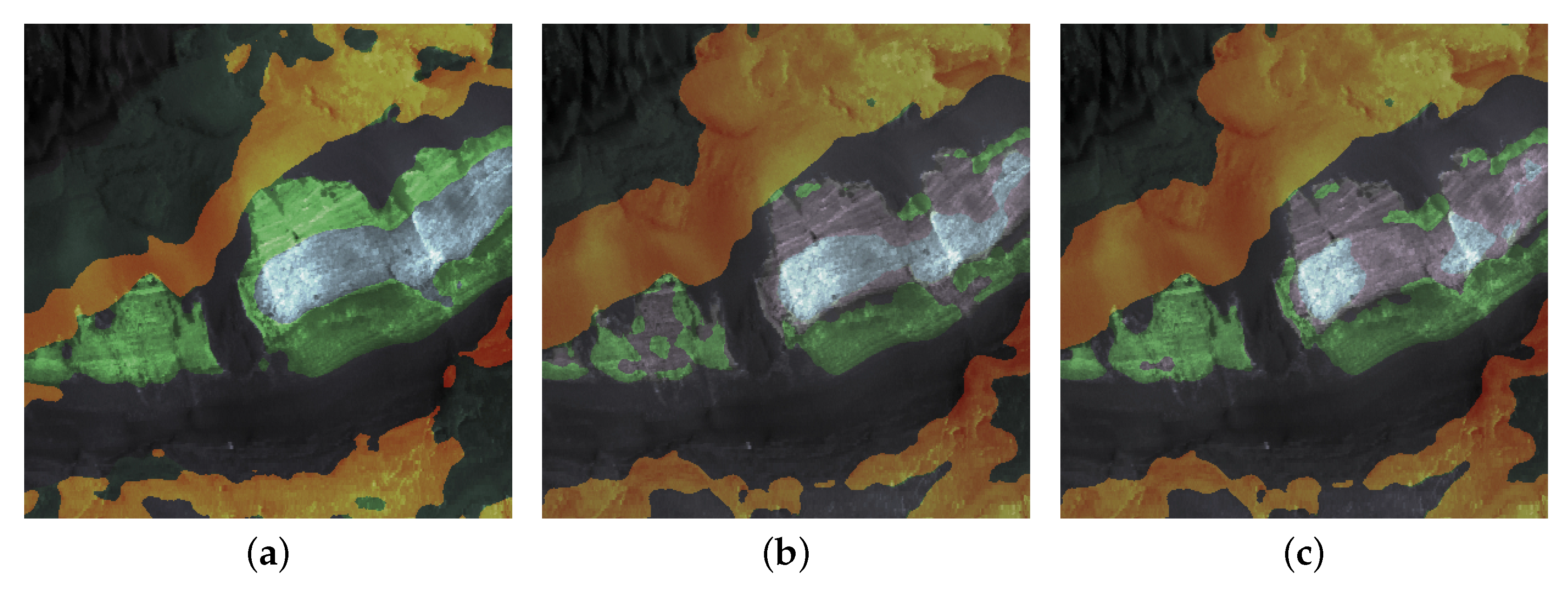
According to the results of all metrics (Calinski–Harabasz and Davies–Bouldin), the UMAP combined with the K-Means cluster procedure clearly shows the best scores (compare Table 1 and Table A1). At the same time, it has a moderate computing time compared with the PCA calculations. Consequently, this method was selected and was optimized with respect to the cluster size. The aforementioned metrics for evaluating clustering performance can be applied. Figure 4 shows that a cluster size of 3, 4 or 6 is proposed for the individual datasets investigated in this study. The final cluster map overlaid on the images is shown in Figure 6a for FRT0001c71b.
Gao et al. [5] used expert maps to assign geological properties to the clusters, in order to relate the clusters to geo-morphological properties of the surface. Similarly, we use the so-called summary products derived by Pelkey et al. [24] and Viviano et al. [25], which retrieve mineralogical information by evaluating specific band structures within the given spectral range. For a detailed description, we refer to Pelkey et al. [24]. We try to determine which minimum set of these products can be used as input features in a random forest model to classify the SCM labeled pixel with a good accuracy. The dataset consisting of the SCMs and its corresponding browse products from image set FRT0001c71b were split into training and test sets using a ratio of 0.25. Applying common feature reduction procedures, it shows that four spectral bands are sufficient without a large loss in prediction accuracy.
Furthermore, we compute permutation importance for feature evaluation using the random forest classifier as an estimator. Our analysis shows that four of the five features of the subsequent list are dominant for all datasets: RBR, R770, BD860_2, BDI1000VIS and R1080. Besides the expected reflectance at 770 nm, the bands in the NIR dominates. Viviano et al. [25] related this to the presence of olivine and pyroxenes. The 860 nm band plays a dominant role in discriminating ferric minerals, such as hematite [25]. The positions of the final features within the spectra are shown in Figure 7; they basically describe the silhouette of the spectra dividing it into four distinct areas. It is plausible to relate these given clusters to geomorphical compositions. Coprates Chasma shows brighter areas, which we can see in Figure 6. According to Loizeau et al. and Fueten et al. [36,58] light tone areas could exhibit hydrated minerals and consist of hydrated minerals. Further analysis has to show if such clusters can be more diversified depending on the different minerals.
It is, therefore, now feasible to apply the CaSSIS filter response to the spectral data. We calculate four new CaSSIS-like features. Within the wavelength range of CaSSIS, there are electronic transitions and crystal field effects caused by the presence of ferrous Fe2+ iron-bearing minerals that produce diagnostic absorptions between 700 and 1100 nm (e.g., mafic minerals such as olivine and pyroxene). The CaSSIS sensitivity range also includes diagnostic broad absorptions which arise from intervalence charge-transfer transitions of ferric iron Fe3+ and O2− and are present in altered ferric (Fe3+) iron-bearing minerals (e.g., hematite, nontronite, etc.) [26].
The CaSSIS filters were selected to give good overlap with the HiRISE bandpasses but splitting the NIR bandpass in HiRISE into two separate bandpasses (RED and NIR in CaSSIS) is needed to improve mineralogical distinction. The HIRISE filters are given in McEwen et al. [1], while the CaSSIS filters are described in Thomas et al. [3] or Gambicorti et al. [59,60]. Table A2 in the Appendix C provides a summary of the bandpasses. The effective central wavelengths of the CaSSIS filters (taking into account the optical transmission and detector response) are also given.
Similarly we apply a K-Means algorithm on the selected summary products and on the four CaSSIS features dataset to generate similar cluster maps. These maps are shown in Figure 6b,c. A strong visual correlation between these maps can be clearly seen, which enables principally to retrieve basic information about both the surface structure and the Fe-mineralogy.
5. Conclusions
In this paper, a simple fast method is proposed to derive spectral clusters from hyperspectral data in the visible wavelength range. The analyses show that the UMAP algorithm in combination with the K-Means clustering method provides results quickly and, based on common cluster metrics, provides comparable or even better results than other proposed methods. With respect to the evaluation and combination of large hyperspectral datasets, this can be a decisive factor.
Comparison with the similarly generated maps based on summary products demonstrate the high information content of four bands partially from NIR, discriminating especially the Fe mineralogy within that area. The reduced number of relevant bands and a proposed cluster size between 3 and 6 confirm that the four CaSSIS filter bands were a reasonable selection sufficient for mineralogical analyses (at least for the Coprates Chasma region) at visible wavelengths.
This proposed methodology can also be utilized to vary filter parameters and to propose new settings for future missions. Additionally, it is possible to use this procedure to generate “new” or slightly different combinations of spectral bands resulting in different image browse product.
It must be emphasized that the results can depend strongly on the data selection, the preprocessing and the signal-to-noise ratio. Thus, this procedure should rather be used as an aid with other analyses. Therefore, further iterative optimization of the procedure regarding robustness and the extension of the analyses to the geologically more relevant wavelengths in the NIR range are planned.
Author Contributions
Writing—original draft, M.F. and A.P.; Writing—review & editing, N.T., A.P.R. and B.E. All authors contributed substantial work at every stage of this publication. All authors have read and agreed to the published version of the manuscript.
Funding
A.P.R. has been supported by the Europlanet H204 RI and has received funding from the European Union’s Horizon 2020 research and innovation programme under grant agreement No. 871149.
Data Availability Statement
The CRISM data used here are available through the PDS Geoscience Node (https://ode.rsl.wustl.edu (accessed on 1 September 2021)). The CaSSIS dataset is available from the Planetary Science Archive (PSA) of the European Space Agency (https://archives.esac.esa.int/psa/#!Home%20View (accessed on 1 September 2021)).
Conflicts of Interest
The authors declare no conflict of interest.
Abbreviations
The following abbreviations are commonly used in this manuscript:
| CaSSIS | Color and Stereo Surface Imaging System |
| CH | Calinski–Harabasz |
| CRISM | Compact Reconnaissance Imaging Spectrometer |
| DB | Davies–Bouldin |
| GMM | Gaussian Mixture model |
| HiRISE | High Resolution Imaging Science Experiment |
| MRO | Mars Reconnaissance Orbiter |
| MTRDR | Map-projected Targeted Reduced Data Record |
| PCA | Principal omponent analysis |
| SC | Silhouette Coefficient |
| SCM | Spectral Cluster Map |
| SOM | Self-organizing map |
| t-SNE | t-distributed Stochastic Neighbor Embedding |
| TGO | ExoMars Trace Gas Orbiter |
| UMAP | Uniform Manifold Approximation and Projection |
Appendix A

Table A1.
Mean of the Davies–Bouldin criterion over a range of three to seven clusters, split by method and region. The best score for each dataset is in bold.
Table A1.
Mean of the Davies–Bouldin criterion over a range of three to seven clusters, split by method and region. The best score for each dataset is in bold.
| Regions | |||
|---|---|---|---|
| Methods | FRT0000d3a4 | FRT0001c479 | FRT0001c71b |
| Autoencoder + K-Means | 0.8775 | 0.9128 | 0.7967 |
| Autoencoder + GMM | 2.9242 | 2.2085 | 0.8964 |
| Autoencoder + SOM | 1.2979 | 1.1723 | 0.9601 |
| Autoencoder + Fuzzy-c-Means | 1.0237 | 0.9387 | 0.8412 |
| PCA + K-Means | 0.8678 | 0.9009 | 0.8000 |
| PCA + GMM | 1.9057 | 1.7879 | 0.8214 |
| PCA + SOM | 1.2301 | 1.1618 | 0.9572 |
| PCA + Fuzzy-c-Means | 1.0105 | 0.9256 | 0.8434 |
| t-SNE + K-Means | 0.8332 | 0.8347 | 0.8369 |
| t-SNE + GMM | 0.8454 | 0.8614 | 0.8660 |
| t-SNE + SOM | 0.9658 | 0.9936 | 1.0490 |
| t-SNE + Fuzzy-c-Means | 0.8673 | 0.8438 | 0.8507 |
| UMAP + K-Means | 0.7425 | 0.6971 | 0.6523 |
| UMAP + GMM | 0.7322 | 0.7178 | 0.7142 |
| UMAP + SOM | 1.0230 | 0.8936 | 0.7817 |
| UMAP + Fuzzy-c-Means | 0.7682 | 0.7178 | 0.6542 |
Appendix B. Citation of PDS Data Products
PDS3 data products cited in this paper as part of https://doi.org/10.17189/1519470 (accessed on 1 September 2021) have the following PDS3 DATA_SET_ID:PRODUCT_IDs:
FRT0000d3a4
FRT0001c479
FRT0001c71b
Appendix C. HiRISE and CaSSIS Filter Bandpasses
Table A2.
A comparison of the HiRISE and CaSSIS filter bandpasses. HiRISE data taken from McEwen et al. [1]. The filters are not perfect top-hat functions and cut-off values can be +/−5 nm depending on the definition used.
Table A2.
A comparison of the HiRISE and CaSSIS filter bandpasses. HiRISE data taken from McEwen et al. [1]. The filters are not perfect top-hat functions and cut-off values can be +/−5 nm depending on the definition used.
| HiRISE Name | HiRISE Color Band | CaSSIS Name | CaSSIS Color Band | CaSSIS Effective Central Wavelength |
|---|---|---|---|---|
| BG | <580 nm | BLU | <570 nm | 494 nm |
| RED | 570–830 nm | PAN | 550–800 nm | 678 nm |
| NIR | >790 nm | RED | 785–880 nm | 836 nm |
| NIR | >870 nm | 939 nm |
References
- McEwen, A.S.; Eliason, E.M.; Bergstrom, J.W.; Bridges, N.T.; Hansen, C.J.; Delamere, W.A.; Grant, J.A.; Gulick, V.C.; Herkenhoff, K.E.; Keszthelyi, L.; et al. Mars reconnaissance orbiter’s high resolution imaging science experiment (HiRISE). J. Geophys. Res. Planets 2007, 112, E05S02. [Google Scholar] [CrossRef] [Green Version]
- Murchie, S.; Arvidson, R.; Bedini, P.; Beisser, K.; Bibring, J.P.; Bishop, J.; Boldt, J.; Cavender, P.; Choo, T.; Clancy, R.T.; et al. Compact Reconnaissance Imaging Spectrometer for Mars (CRISM) on Mars Reconnaissance Orbiter (MRO). J. Geophys. Res. Planets 2007, 112, E05S02. [Google Scholar] [CrossRef]
- Thomas, N.; Cremonese, G.; Ziethe, R.; Gerber, M.; Brändli, M.; Bruno, G.; Erismann, M.; Gambicorti, L.; Gerber, T.; Ghose, K.; et al. The Colour and Stereo Surface Imaging System (CaSSIS) for the ExoMars Trace Gas Orbiter. Space Sci. Rev. 2017, 212, 1897–1944. [Google Scholar] [CrossRef] [Green Version]
- Schubert, G. Treatise on Geophysics; Elsevier: Amsterdam, The Netherlands, 2015; ISBN 978-0-444-53803-1. [Google Scholar]
- Gao, A.F.; Rasmussen, B.; Kulits, P.; Scheller, E.L.; Greenberger, R.; Ehlmann, B.L. Generalized Unsupervised Clustering of Hyperspectral Images of Geological Targets in the Near Infrared. In Proceedings of the IEEE/CVF Conference on Computer Vision and Pattern Recognition, Nashville, TN, USA, 20–25 June 2021; pp. 4294–4303. [Google Scholar]
- Timmerman, M.E. Principal Component Analysis. J. Am. Stat. Assoc. 2003, 98, 1082–1083. [Google Scholar] [CrossRef]
- Martel, E.; Lazcano, R.; López, J.; Madroñal, D.; Salvador, R.; López, S.; Juarez, E.; Guerra, R.; Sanz, C.; Sarmiento, R. Implementation of the Principal Component Analysis onto High-Performance Computer Facilities for Hyperspectral Dimensionality Reduction: Results and Comparisons. Remote Sens. 2018, 10, 864. [Google Scholar] [CrossRef] [Green Version]
- Rodarmel, C.; Shan, J. Principal component analysis for hyperspectral image classification. Surv. Land Inf. Sci. 2002, 62, 115–122. [Google Scholar]
- Melit Devassy, B.; George, S.; Nussbaum, P. Unsupervised Clustering of Hyperspectral Paper Data Using t-SNE. J. Imaging 2020, 6, 29. [Google Scholar] [CrossRef]
- Pouyet, E.; Rohani, N.; Katsaggelos, A.K.; Cossairt, O.; Walton, M. Innovative data reduction and visualization strategy for hyperspectral imaging datasets using t-SNE approach. Pure Appl. Chem. 2018, 90, 493–506. [Google Scholar] [CrossRef]
- Song, W.; Wang, L.; Liu, P.; Choo, K.K.R. Improved t-SNE based manifold dimensional reduction for remote sensing data processing. Multimed. Tools Appl. 2019, 78, 4311–4326. [Google Scholar] [CrossRef]
- Kohonen, T. Adaptive, associative, and self-organizing functions in neural computing. Appl. Opt. 1987, 26, 4910–4918. [Google Scholar] [CrossRef]
- Picollo, M.; Cucci, C.; Casini, A.; Stefani, L. Hyper-Spectral Imaging Technique in the Cultural Heritage Field: New Possible Scenarios. Sensors 2020, 20, 2843. [Google Scholar] [CrossRef] [PubMed]
- Wander, L.; Vianello, A.; Vollertsen, J.; Westad, F.; Braun, U.; Paul, A. Exploratory analysis of hyperspectral FTIR data obtained from environmental microplastics samples. Anal. Methods 2020, 12, 781–791. [Google Scholar] [CrossRef]
- D’Amore, M.; Padovan, S. Chapter 7—Automated surface mapping via unsupervised learning and classification of Mercury Visible–Near-Infrared reflectance spectra. In Machine Learning for Planetary Science; Helbert, J., D’Amore, M., Aye, M., Kerner, H., Eds.; Elsevier: Amsterdam, The Netherlands, 2022; pp. 131–149. ISBN 978-0-12-818721-0. [Google Scholar]
- Ferrer-Font, L.; Mayer, J.U.; Old, S.; Hermans, I.F.; Irish, J.; Price, K.M. High-Dimensional Data Analysis Algorithms Yield Comparable Results for Mass Cytometry and Spectral Flow Cytometry Data. Cytom. Part A 2020, 97, 824–831. [Google Scholar] [CrossRef]
- Yang, Y.; Sun, H.; Zhang, Y.; Zhang, T.; Gong, J.; Wei, Y.; Duan, Y.G.; Shu, M.; Yang, Y.; Wu, D.; et al. Dimensionality reduction by UMAP reinforces sample heterogeneity analysis in bulk transcriptomic data. Cell Rep. 2021, 36, 109442. [Google Scholar] [CrossRef] [PubMed]
- Zambon, F.; Carli, C.; Wright, J.; Rothery, D.; Altieri, F.; Massironi, M.; Capaccioni, F.; Cremonese, G. Spectral units analysis of quadrangle H05-Hokusai on Mercury. J. Geophys. Res. Planets 2022, 27, e2021JE006918. [Google Scholar] [CrossRef]
- Massironi, M.; Rossi, A.P.; Wright, J.; Zambon, F.; Poheler, C.; Giacomini, L.; Carli, C.; Ferrari, S.; Semenzato, A.; Luzzi, E.; et al. From Morpho-Stratigraphic to Geo(Spectro)-Stratigraphic Units: The PLANMAP Contribution. In Proceedings of the 2021 Annual Meeting of Planetary Geologic Mappers, Virtual, 14–15 June 2021; Volume 2610, p. 7045. Available online: https://ui.adsabs.harvard.edu/abs/2021LPICo2610.7045M (accessed on 31 March 2022).
- Semenzato, A.; Massironi, M.; Ferrari, S.; Galluzzi, V.; Rothery, D.A.; Pegg, D.L.; Pozzobon, R.; Marchi, S. An Integrated Geologic Map of the Rembrandt Basin, on Mercury, as a Starting Point for Stratigraphic Analysis. Remote Sens. 2020, 12, 3213. [Google Scholar] [CrossRef]
- Giacomini, L.; Carli, C.; Zambon, F.; Galluzzi, V.; Ferrari, S.; Massironi, M.; Altieri, F.; Ferranti, L.; Palumbo, P.; Capaccioni, F. Integration between morphological and spectral characteristics for the geological map of Kuiper quadrangle (H06). In Proceedings of the EGU General Assembly Conference, Online, 19–30 April 2021; p. EGU21-15052. [Google Scholar]
- Pajola, M.; Lucchetti, A.; Semenzato, A.; Poggiali, G.; Munaretto, G.; Galluzzi, V.; Marzo, G.; Cremonese, G.; Brucato, J.; Palumbo, P.; et al. Lermontov crater on Mercury: Geology, morphology and spectral properties of the coexisting hollows and pyroclastic deposits. Planet. Space Sci. 2021, 195, 105136. [Google Scholar] [CrossRef]
- Seelos, F. Mars Reconnaissance Orbiter Compact Reconnaissance Imaging Spectrometer for Mars Map-Projected Targeted Reduced Data Record; MRO-M-CRISM-5-RDR-MPTARGETED-V1.0; NASA Planetary Data System: St. Louis, MO, USA, 2016. [CrossRef]
- Pelkey, S.M.; Mustard, J.F.; Murchie, S.; Clancy, R.T.; Wolff, M.; Smith, M.; Milliken, R.; Bibring, J.P.; Gendrin, A.; Poulet, F.; et al. CRISM multispectral summary products: Parameterizing mineral diversity on Mars from reflectance. J. Geophys. Res. Planets 2007, 112, E08S14. [Google Scholar] [CrossRef]
- Viviano, C.E.; Seelos, F.P.; Murchie, S.L.; Kahn, E.G.; Seelos, K.D.; Taylor, H.W.; Taylor, K.; Ehlmann, B.L.; Wiseman, S.M.; Mustard, J.F.; et al. Revised CRISM spectral parameters and summary products based on the currently detected mineral diversity on Mars. J. Geophys. Res. Planets 2014, 119, 1403–1431. [Google Scholar] [CrossRef] [Green Version]
- Tornabene, L.L.; Seelos, F.P.; Pommerol, A.; Thomas, N.; Caudill, C.M.; Becerra, P.; Bridges, J.C.; Byrne, S.; Cardinale, M.; Chojnacki, M.; et al. Image Simulation and Assessment of the Colour and Spatial Capabilities of the Colour and Stereo Surface Imaging System (CaSSIS) on the ExoMars Trace Gas Orbiter. Space Sci. Rev. 2018, 214, 18. [Google Scholar] [CrossRef]
- Parkes Bowen, A.; Mandon, L.; Bridges, J.; Quantin-Nataf, C.; Tornabene, L.; Page, J.; Briggs, J.; Thomas, N.; Cremonese, G. Using band ratioed CaSSIS imagery and analysis of fracture morphology to characterise Oxia Planum’s clay-bearing unit. In Proceedings of the European Planetary Science Congress, Virtual, 21 September–9 October 2020; p. EPSC2020-877. [Google Scholar] [CrossRef]
- Parkes Bowen, A.; Bridges, J.; Tornabene, L.; Mandon, L.; Quantin-Nataf, C.; Patel, M.R.; Thomas, N.; Cremonese, G.; Munaretto, G.; Pommerol, A.; et al. A CaSSIS and HiRISE map of the Clay-bearing Unit at the ExoMars 2022 landing site in Oxia Planum. Planet. Space Sci. 2022, 214, 105429. [Google Scholar] [CrossRef]
- Thomas, N.; Pommerol, A.; Almeida, M.; Read, M.; Cremonese, G.; Simioni, E.; Munaretto, G.; Weigel, T. Absolute calibration of the Colour and Stereo Surface Imaging System (CaSSIS). Planet. Space Sci. 2021, 211, 105394. [Google Scholar] [CrossRef]
- Tulyakov, S.; Ivanov, A.; Thomas, N.; Roloff, V.; Pommerol, A.; Cremonese, G.; Weigel, T.; Fleuret, F. Geometric calibration of Colour and Stereo Surface Imaging System of ESA’s Trace Gas Orbiter. Adv. Space Res. 2018, 61, 487–496. [Google Scholar] [CrossRef] [Green Version]
- Weitz, C.M.; Irwin III, R.P.; Chuang, F.C.; Bourke, M.C.; Crown, D.A. Formation of a terraced fan deposit in Coprates Catena, Mars. Icarus 2006, 184, 436–451. [Google Scholar] [CrossRef]
- Grindrod, P.M.; Warner, N.; Hobley, D.; Schwartz, C.; Gupta, S. Stepped fans and facies-equivalent phyllosilicates in Coprates Catena, Mars. Icarus 2018, 307, 260–280. [Google Scholar] [CrossRef]
- Chojnacki, M.; Hynek, B.M. Geological context of water-altered minerals in Valles Marineris, Mars. J. Geophys. Res. Planets 2008, 113, E12005. [Google Scholar] [CrossRef] [Green Version]
- Weitz, C.M.; Bishop, J.L. Stratigraphy and formation of clays, sulfates, and hydrated silica within a depression in Coprates Catena, Mars. J. Geophys. Res. Planets 2016, 121, 805–835. [Google Scholar] [CrossRef] [Green Version]
- Murchie, S.L.; Bibring, J.P.; Arvidson, R.E.; Bishop, J.L.; Carter, J.; Ehlmann, B.L.; Langevin, Y.; Mustard, J.F.; Poulet, F.; Riu, L.; et al. Visible to Short-Wave Infrared Spectral Analyses of Mars from Orbit Using CRISM and OMEGA. In Remote Compositional Analysis: Techniques for Understanding Spectroscopy, Mineralogy, and Geochemistry of Planetary Surfaces; Cambridge Planetary Science; Cambridge University Press: Cambridge, UK, 2019; pp. 453–483. [Google Scholar] [CrossRef]
- Fueten, F.; Racher, H.; Stesky, R.; MacKinnon, P.; Hauber, E.; McGuire, P.; Zegers, T.; Gwinner, K. Structural analysis of interior layered deposits in Northern Coprates Chasma, Mars. Earth Planet. Sci. Lett. 2010, 294, 343–356. [Google Scholar] [CrossRef] [Green Version]
- Buczkowski, D.; Seelos, K.; Viviano, C.; Murchie, S.; Seelos, F.; Malaret, E.; Hash, C. Anomalous Phyllosilicate-Bearing Outcrops South of Coprates Chasma: A Study of Possible Emplacement Mechanisms. J. Geophys. Res. Planets 2020, 125, e2019JE006043. [Google Scholar] [CrossRef]
- Le Deit, L.; Flahaut, J.; Quantin, C.; Hauber, E.; Mège, D.; Bourgeois, O.; Gurgurewicz, J.; Massé, M.; Jaumann, R. Extensive surface pedogenic alteration of the Martian Noachian crust evidenced by plateau phyllosilicates around Valles Marineris. J. Geophys. Res. 2012, 117, E00J05. [Google Scholar] [CrossRef]
- Kovenko, V.; Bogach, I. A Comprehensive Study of Autoencoders’ Applications Related to Images. In Proceedings of the IT&I Workshops, Kyiv, Ukraine, 2–3 December 2020. [Google Scholar]
- Le, Q.V. A tutorial on deep learning part 2: Autoencoders, convolutional neural networks and recurrent neural networks. Google Brain 2015, 20, 1–20. [Google Scholar]
- Van der Maaten, L.; Hinton, G. Visualizing data using t-SNE. J. Mach. Learn. Res. 2008, 9, 2579–2625. [Google Scholar]
- Kullback, S.; Leibler, R.A. On Information and Sufficiency. Ann. Math. Stat. 1951, 22, 79–86. [Google Scholar] [CrossRef]
- McInnes, L.; Healy, J.; Melville, J. UMAP: Uniform Manifold Approximation and Projection for Dimension Reduction. arXiv 2018, arXiv:1802.03426. [Google Scholar]
- Allaoui, M.; Kherfi, M.L.; Cheriet, A. Considerably Improving Clustering Algorithms Using UMAP Dimensionality Reduction Technique: A Comparative Study. In Image and Signal Processing; El Moataz, A., Mammass, D., Mansouri, A., Nouboud, F., Eds.; Springer International Publishing: Cham, Switzerland, 2020; pp. 317–325. [Google Scholar]
- Vermeulen, M.; Smith, K.; Eremin, K.; Rayner, G.; Walton, M. Application of Uniform Manifold Approximation and Projection (UMAP) in spectral imaging of artworks. Spectrochim. Acta Part A Mol. Biomol. Spectrosc. 2021, 252, 119547. [Google Scholar] [CrossRef]
- MacQueen, J. Some methods for classification and analysis of multivariate observations. In Proceedings of the 5th Berkeley Symposium on Mathematical Statistics and Probability, Oakland, CA, USA; 1967; Volume 1, pp. 281–297. [Google Scholar]
- Bishop, C.M.; Nasrabadi, N.M. Pattern Recognition and Machine Learning; Springer: Berlin/Heidelberg, Germany, 2006; Volume 4, ISBN 978-0-387-31073-2. [Google Scholar]
- Bezdek, J.C.; Ehrlich, R.; Full, W. FCM: The fuzzy c-means clustering algorithm. Comput. Geosci. 1984, 10, 191–203. [Google Scholar] [CrossRef]
- Kohonen, T. Self-Organizing Maps; Springer: Berlin/Heidelberg, Germany, 1997; ISBN 978-3-642-97966-8. [Google Scholar]
- Bioucas-Dias, J.M.; Nascimento, J.M.P. Hyperspectral Subspace Identification. IEEE Trans. Geosci. Remote Sens. 2008, 46, 2435–2445. [Google Scholar] [CrossRef] [Green Version]
- Pedregosa, F.; Varoquaux, G.; Gramfort, A.; Michel, V.; Thirion, B.; Grisel, O.; Blondel, M.; Prettenhofer, P.; Weiss, R.; Dubourg, V.; et al. Scikit-learn: Machine Learning in Python. J. Mach. Learn. Res. 2011, 12, 2825–2830. [Google Scholar]
- Sklearn-Som v. 1.1.0 Master Documentation. Available online: https://sklearn-som.readthedocs.io/en/latest/ (accessed on 17 March 2022).
- Dias, M.L.D. Fuzzy-c-Means: An Implementation of Fuzzy C-Means Clustering Algorithm; Zenodo: Geneva, Switzerland, 2019. [Google Scholar] [CrossRef]
- Caliński, T.; Harabasz, J. A dendrite method for cluster analysis. Commun. Stat.-Theory Methods 1974, 3, 1–27. [Google Scholar] [CrossRef]
- Davies, D.L.; Bouldin, D.W. A Cluster Separation Measure. IEEE Trans. Pattern Anal. Mach. Intell. 1979, PAMI-1, 224–227. [Google Scholar] [CrossRef]
- Rousseeuw, P.J. Silhouettes: A graphical aid to the interpretation and validation of cluster analysis. J. Comput. Appl. Math. 1987, 20, 53–65. [Google Scholar] [CrossRef] [Green Version]
- Milligan, G.W.; Cooper, M.C. An examination of procedures for determining the number of clusters in a data set. Psychometrika 1985, 50, 159–179. [Google Scholar] [CrossRef]
- Loizeau, D.; Quantin-Nataf, C.; Carter, J.; Flahaut, J.; Thollot, P.; Lozac’h, L.; Millot, C. Quantifying widespread aqueous surface weathering on Mars: The plateaus south of Coprates Chasma. Icarus 2018, 302, 451–469. [Google Scholar] [CrossRef]
- Gambicorti, L.; Piazza, D.; Gerber, M.; Pommerol, A.; Roloff, V.; Ziethe, R.; Zimmermann, C.; Da Deppo, V.; Cremonese, G.; Veltroni, I.F.; et al. Thin-film optical pass band filters based on new photo-lithographic process for CaSSIS FPA detector on Exomars TGO mission: Development, integration, and test. In Advances in Optical and Mechanical Technologies for Telescopes and Instrumentation II; International Society for Optics and Photonics: Bellingham, WA, USA, 2016; Volume 9912, p. 99122Y. [Google Scholar]
- Gambicorti, L.; Piazza, D.; Pommerol, A.; Roloff, V.; Gerber, M.; Ziethe, R.; El-Maarry, M.R.; Weigel, T.; Johnson, M.; Vernani, D.; et al. First light of Cassis: The stereo surface imaging system onboard the exomars TGO. In Proceedings of the International Conference on Space Optics—ICSO 2016, Biarritz, France, 18–21 October 2016; International Society for Optics and Photonics: Bellingham, WA, USA, 2017; Volume 10562, p. 105620A. [Google Scholar]
Figure 1.
Location map of the used cubes in the present work. Left: color-coded MGS MOLA hillshade over Coprates Chasma and surrounding plateau; the white outline indicates the extent of the right panel (data). Right: location of the three overlapping CRISM observations used here; the background imagery consists of HRSC Level4 Nadir imagery, orbit h7201.

Figure 2.
Examples of produced spectral cluster maps with a predefined number of 10 clusters from the FRT0001c71b dataset. (a) Autoencoder + GMM; (b) PCA + K-Means; (c) UMAP + Fuzzy-c-Means.
Figure 2.
Examples of produced spectral cluster maps with a predefined number of 10 clusters from the FRT0001c71b dataset. (a) Autoencoder + GMM; (b) PCA + K-Means; (c) UMAP + Fuzzy-c-Means.

Figure 3.
Calinski–Harabasz and Davies–Bouldin index as a function of the number of clusters for the FRT0001c71b dataset. Each subfigure (a–c) represents quantitative analysis for the same combinations of the dimensionality reduction technique and clustering algorithm as in Figure 2.
Figure 3.
Calinski–Harabasz and Davies–Bouldin index as a function of the number of clusters for the FRT0001c71b dataset. Each subfigure (a–c) represents quantitative analysis for the same combinations of the dimensionality reduction technique and clustering algorithm as in Figure 2.

Figure 4.
Silhouette Score UMAP + K-Means as a function of the number of clusters for all three datasets.
Figure 4.
Silhouette Score UMAP + K-Means as a function of the number of clusters for all three datasets.

Figure 5.
Silhouette coefficient for the identified number of clusters for each dataset across all examined methods. The scores are grouped by clustering algorithm. The UMAP algorithm has the highest SC score in all but one case. (a) FRT0000d3a4; (b) FRT0001c479; (c) FRT0001c71b.
Figure 5.
Silhouette coefficient for the identified number of clusters for each dataset across all examined methods. The scores are grouped by clustering algorithm. The UMAP algorithm has the highest SC score in all but one case. (a) FRT0000d3a4; (b) FRT0001c479; (c) FRT0001c71b.


Figure 6.
Spectral cluster maps generated for a configuration of six clusters and the FRT0001c71b dataset. In (a) Spectral cluster map, UMAP + K-Means is applied, in (b) Cluster map based on four selected summary products and in (c) Cluster map based on CaSSIS bands.
Figure 6.
Spectral cluster maps generated for a configuration of six clusters and the FRT0001c71b dataset. In (a) Spectral cluster map, UMAP + K-Means is applied, in (b) Cluster map based on four selected summary products and in (c) Cluster map based on CaSSIS bands.

Figure 7.
Spectral information with supporting bands, dividing area into four distinct ranges.

Table 1.
Mean of the Calinski–Harabasz criterion over a range of 3 to 7 clusters, split by method and region. The best score for each dataset is in bold.
Table 1.
Mean of the Calinski–Harabasz criterion over a range of 3 to 7 clusters, split by method and region. The best score for each dataset is in bold.
| Regions | |||
|---|---|---|---|
| Methods | FRT0000d3a4 | FRT0001c479 | FRT0001c71b |
| Autoencoder + K-Means | 96.371 | 135.768 | 221.408 |
| Autoencoder + GMM | 49.838 | 62.005 | 185.458 |
| Autoencoder + SOM | 69.396 | 108.513 | 192.581 |
| Autoencoder + Fuzzy-c-Means | 81.773 | 133.995 | 214.217 |
| PCA + K-Means | 97.718 | 138.611 | 220.849 |
| PCA + GMM | 50.756 | 82.344 | 202.702 |
| PCA + SOM | 71.086 | 110.939 | 192.436 |
| PCA + Fuzzy-c-Means | 83.132 | 136.640 | 213.769 |
| t-SNE + K-Means | 137.141 | 138.955 | 138.998 |
| t-SNE + GMM | 132.889 | 128.090 | 127.752 |
| t-SNE + SOM | 120.052 | 114.351 | 113.640 |
| t-SNE + Fuzzy-c-Means | 134.679 | 138.300 | 137.684 |
| UMAP + K-Means | 207.836 | 246.825 | 284.543 |
| UMAP + GMM | 178.341 | 216.898 | 224.978 |
| UMAP + SOM | 162.585 | 198.219 | 222.445 |
| UMAP + Fuzzy-c-Means | 206.015 | 245.274 | 284.117 |
Publisher’s Note: MDPI stays neutral with regard to jurisdictional claims in published maps and institutional affiliations. |
© 2022 by the authors. Licensee MDPI, Basel, Switzerland. This article is an open access article distributed under the terms and conditions of the Creative Commons Attribution (CC BY) license (https://creativecommons.org/licenses/by/4.0/).
Share and Cite
MDPI and ACS Style
Fernandes, M.; Pletl, A.; Thomas, N.; Rossi, A.P.; Elser, B. Generation and Optimization of Spectral Cluster Maps to Enable Data Fusion of CaSSIS and CRISM Datasets. Remote Sens. 2022, 14, 2524. https://doi.org/10.3390/rs14112524
AMA Style
Fernandes M, Pletl A, Thomas N, Rossi AP, Elser B. Generation and Optimization of Spectral Cluster Maps to Enable Data Fusion of CaSSIS and CRISM Datasets. Remote Sensing. 2022; 14(11):2524. https://doi.org/10.3390/rs14112524
Chicago/Turabian StyleFernandes, Michael, Alexander Pletl, Nicolas Thomas, Angelo Pio Rossi, and Benedikt Elser. 2022. "Generation and Optimization of Spectral Cluster Maps to Enable Data Fusion of CaSSIS and CRISM Datasets" Remote Sensing 14, no. 11: 2524. https://doi.org/10.3390/rs14112524
Note that from the first issue of 2016, this journal uses article numbers instead of page numbers. See further details here.