
The Remotely and Directly Obtained Results of Glaciological Studies on King George Island: A Review


Institute of Biochemistry and Biophysics, Polish Academy of Sciences, 02-106 Warsaw, Poland
*
Author to whom correspondence should be addressed.
Remote Sens. 2022, 14(12), 2736; https://doi.org/10.3390/rs14122736
Submission received: 19 April 2022
/
Revised: 23 May 2022
/
Accepted: 2 June 2022
/
Published: 7 June 2022
(This article belongs to the Special Issue Applications of Remote Sensing in Glaciology)
Abstract
:Climate warming has become indisputable, and it is now crucial to increase our understanding of both the mechanisms and consequences of climate change. The Antarctic region is subjected to substantial changes, the trends of which have been recognized for several decades. In the South Shetland Islands, the most visible effect of climate change is progressive deglaciation. The following review focuses on past glaciological studies conducted on King George Island (KGI). The results of collected cryosphere element observations are discussed herein in a comprehensive manner. Our analysis showed that there is a lack of temporal as well as spatial continuity for studies on the basic mass balance parameters on the entire KGI ice dome and only Bellingshausen Dome has a relatively long history of data collection. The methodologies of past work, which have improved over time, are also discussed. When studying the glacier front fluctuations, the authors most frequently use a 1956 aerial photography as reference ice coverage. This was the case for seven papers, while other sources are seldomly mentioned. In other papers as many as 41 other sources were used, and therefore comparison to photos taken up to 60 years later can give misleading trends, as small glaciers may have both advanced and retreated in that time. In the case of glacial velocities there is also an apparent lack of consistency, as different glaciers were indicated as the fastest on KGI. Only Lange, Anna, Crystal, Eldred, and eastern part of Usher glaciers were determined by more than one author as the fastest. Additionally, there are gaps in the KGI Ground Penetrating Radar (GPR) survey area, which includes three ice domes: the Warszawa Icefield, the Krakow Icefield, and eastern part of King George Island. Ideas for further work on the topic are also suggested, allowing for easier access to data and thus contributing to a better understanding of glacier development mechanisms.
1. Introduction
Polar regions are considered very sensitive indicators of climate change. Although knowledge on this subject is common, the relationships between climate change and the recession and transgression of glaciers are complicated [1]. Numerous research studies have focused on these relationships while attempting to explain the mechanisms by which the climate impacts the state of ice in polar regions [1,2,3,4,5,6,7].
To completely understand the complexity of the phenomena and processes occurring in glaciers and their relationship with the natural environment, glaciers should be considered dynamic open systems, i.e., systems of internally coordinated elements with a specific structure [8]. The main feature of a glacier system is the mass exchange process consisting of mass transfer and release [9].
The basic building material in a glacier is ice; glaciers form through the transformation of accumulated snow. Ablation is a process that involves the loss of glacier mass during melting, along with meltwater outflow, calving, drifting, and sublimation [1]. The difference between the amount of accumulated glacial material in the form of snow or ice and the lost mass is called the glacier mass balance [6]. By recognizing this mass balance and determining its factors, we can set the course of modern glacier evolution research and recognize the climatic conditions that influenced the existence of glaciers in the Pleistocene [8]. When determining glacial mass balance, geodetic measurements are also carried out. To provide information on changes in glacier surface heights over time, various digital elevation models (DEMs) have been compared. The relevant data sources include Global Positioning System (GPS) measurements, laser scanning data, aerial and satellite photogrammetry, and digitized topographic maps. Less frequently used techniques for mass balance estimations include climatological and hydrological methods and ice mass flow velocity measurements taken in glacial cross-sections located below the equilibrium line (EL) [1,9].
Glacial mass balance and the processes controlling its fluctuations are key factors to address when aiming to understand and forecast climate change. Monitoring mass balance components is one of the fundamental activities of glaciological research. Locally, in an ice basin, stored snow and ice affect the outflow of water from a glacier. On the global scale, glacier volume fluctuations directly affect ocean levels [10]. The mass balance of glaciers depends on climatic conditions. However, integrative relationship is mutual, as the presence of glaciers and ice domes critically impact the atmosphere. Consequently, these interactions lead to weather and climate changes from the local scale to the global scale [6].
In situ studies have many disadvantages, such as high financial outlays and spatial limitations. Practical glacier research methods used in modern glaciological studies include the use of aerial and satellite remote sensing data primarily collected during regional-scale observations [11]. When determining glacier dynamics, a particularly important feature is glacial movement, as this feature is critical in the exchange of glacial mass. Glacial movement allows ice to flow below the EL and affects the shape and surface features of a glacier. It is therefore a fundamental process that must be considered to obtain a complete understanding of the change mechanisms taking place in the cryosphere.
The most commonly used methods for measuring glacier flow involve direct GPS measurements, glacial monitoring using time-lapse surveys and remote sensing techniques utilizing optical and radar satellite images [12]. Due to the different physical characteristics of various glacier components, particularly interesting measurement results can be obtained by using a ground-penetrating radar (GPR), which allows the thickness of snow, firn, and ice to be measured [13]. It is also possible to date annual glacier mass increases and estimate the mass balance size of a glacier using this technique. Applying GPR to polythermal glaciers can help differentiate between temperate and cold ice. In addition, shallow probing allows glacial zones to be separated [14]. However, information obtained using GPR is limited to only the profile line, while satellite radar data (e.g., Synthetic Aperture Radar (SAR)) are related to the glacial surface. Thus, collating GPR and SAR data can provide very valuable information, e.g., glacier mass balance estimations, EL locations, superimposed ice ranges, the water contents in glaciers or the direction of canalized subglacial runoff. When using such methods to estimate the water content in a glacier, it is also possible to determine the polythermal structure of the glacier [14].
In this work, we aim to indicate the state of research on the dynamics of the ice dome located on King George Island (KGI) in the South Shetland archipelago in relation to estimating the mass balance of the icefield, determining the local factors affecting glacier movement, and modelling the glaciers and their responses to external factors. This work will allow us to obtain a complete overview of changes in the local glacial environment and to indicate the functions of its various components. Identifying elements that require further observation may help create a complete dome evolution model covering both the past and the far future.
2. Study Site
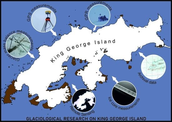
KGI belongs to the South Shetland archipelago and is separated from the Antarctic Peninsula by the Bransfield Strait. The island was discovered in 1819 by William Smith [15,16]. Its area is approximately 1250 km2, and 90% of the island is covered with glaciers (Figure 1) [17]. Due to the relatively easy access to the island, KGI hosts the largest concentration of research activities in Antarctica, with 10 year-round and 3 summer research stations managed by Argentina, Brazil, Chile, China, Ecuador, Peru, Poland, Russia, South Korea, the USA, and Uruguay [18].
KGI is influenced by a subpolar and marine climate. The icefields on the island are influenced by marine climatic conditions, making them more vulnerable to climate change than continental ice caps [19]. The main factor responsible for the observed decrease in the surface areas of these glaciers is the average annual air temperature, which was −2.5 °C from 1948–2011. During this period, large temperature variability was noted; e.g., from 1948–1950, the average annual air temperature was the lowest, amounting to −3.6 °C. A previous data analysis showed significant warming on this island, with the warming rate reaching 0.19 °C per decade (Figure 2A) [20]. A study by Plenzler et al. [21] regarding the local climatic conditions was based on data collected at Arctowski Station from 2013–2017. Data from this period of analysis confirmed the increase in the average annual air temperature, which was recorded at −1.7 °C. As a result, the ice dome on KGI has been reduced by about 7% of the glacial cover area since 1956 [22]. A similar trend has been observed in the glacier mass balance changes. As example, in the period from January 2008 to January 2011, a decrease in the mass balance of the entire icefield of −0.64 ± 0.38 m w.e. a−1 was recorded [23]. The research performed to date on the parameters that compose the mass balance of glaciers on KGI is summarized in Table A1.
3. Mass Balance Parameters
The study of glaciers on the South Shetland Islands began in the 1950s. The first mass balance measurements were taken in 1957 on the Keller Peninsula, near former Base G, by FIDS, marking beginning of the first of three glacier research phases. The second phases was initiated in the late 1970s by Orheim’s observations [24], as discussed in Orheim et al. [25,26]. The third phase began in approximately 1985 with the intensive exploration of the ice domes on KGI and Nelson Island by Brazilian, Chilean, German and Russian scientists [27]. In the following subsections, we provide a review of the research performed to date on the parameters that compose the mass balance of glaciers and the temporal diversity of the ELA courses on KGI glaciers. Summaries of these results are provided in Table A1 and Table A2.
3.1. Ablation
Although accumulation is the collection of processes that build a glacier, in this work, we first discuss the ablation of glaciers on KGI, the observations of which initiated glaciological research on the island. The first glaciological studies performed at KGI, on the Keller Peninsula, were carried out as a part of Base G work from 1957–1960 and focused on measuring the Flagstaff Glacier. The earliest data obtained from these studies presented a summer-season ablation magnitude of 750 mm w.e. a−1 [28]. Observations on Flagstaff Glacier were continued by Stansbury [29]. During the period from 3 February to 21 April of 1959, average ablation of 544 mm w.e. a−1 was observed, while in the summer season of 1959/1960, the recorded ablation was 1310 mm w.e. a−1. Even then, these interseasonal differences in the ablation volume, and hence also in the mass balance, were ascribed to the occurrence of northern winds. In 1960, the atmospheric movement led relatively warm air masses to the KGI, resulting in the higher ablation recorded in the region in this year [27].
Meteorological studies conducted during the austral summer of 1990/1991 were used to obtain surface heat balance and ablation estimations on Ecology Glacier. Near the meteorological station, ablation stakes were read at 100 m a.s.l. The obtained ablation value for the period from 17 December 1990, to 16 January 1991, was 735 mm w.e. [30,31]. After extrapolating this value to the entire ablation season lasting 2.5 months, an ablation magnitude range of 1500–2000 mm w.e. Braun obtained [27], twice the value reported by Orheim and Govorukha [26]. This difference resulted from an assumption by Bintanja [30] of the measuring period, the average temperature of which was warmer by approximately 1.5 °C than the average temperature calculated for a longer period.
Between 2 December 1997 and 12 January 1998, during the research conducted by Braun et al. [32] on the impacts of large-scale atmospheric circulation on the KGI ice dome, ablation measurements were taken from 15 ablative stakes drilled in the profile passing through the Bellingshausen Dome (BD) and Arctowski Icefield (AI) at an altitude of 100 to 385 m a.s.l. In addition, ablation measurement points were located at automatic weather stations (AWSs) at heights of 85, 255, 385 m a.s.l; however, the location of the measurement point at 385 m a.s.l. was moved on 17 December 1997, to a height of 619 m a.s.l. Readings from these stakes were made regularly, every 2–7 days, during the AWS control period. The amount of ablation measured on the lowest-drilled stake was determined to be 383 mm. The collected data also allowed the spatial distributions of ablation on the AI and BD to be determined, amounting to 260 mm w.e. [33].
During the austral summers of 1995/1996, 1997/1998, and 1999/2000, the established AWSs functioned in collecting meteorological data on the BD and AI. Based on the collected materials, Braun et al. [34] published heat balance results on the BD and AI. The created model produced a high correlation coefficient (r2 = 0.99) between the measured and estimated ablation [32], allowing the ablation rates of the investigated glaciers to be estimated. The locations of the AWSs and the daily ablation rates at individual heights are presented in Figure 3. In addition, the average modelled ablation rate was extrapolated over the entire ablation season, i.e., December to March (120 days). The obtained results were approximately 750 mm w.e. a−1 in 1995/96 (AWS A), 1100 mm w.e. a−1 in 1997/98 (AWS 1) and 1150 mm w.e. a−1 in 1999/2000 (AWS 2).
In 2012/2013, field work was carried out to determine the mass balance of the Ecology and Sphinx Glaciers, treating them as one glacial system. Sobota et al. [35] determined the February 2012 ablation value of Ecology Glacier to be >700 mm w.e. a−1. The methodology utilized and research results obtained by Sobota et al. [35] when studying this glacial system are thoroughly described, which refers to glacial mass balance.
The ablation phenomenon progresses with a variable intensity not only within one balance year but also in long-term observations [8]. So far, existing research has focused on determining the ablation sizes of KGI glaciers, and many contributing studies have been performed at irregular intervals. To obtain more precise data, it is necessary to trace the courses of the mass balance components (ablation and accumulation) over a relatively long period while maintaining data continuity. This long-term information could critically increase our knowledge about the processes associated with the glacier-climate relation. Obtaining such data also improves the function of models that predict future glacier changes [36].
3.2. Accumulation
From 1985–1992, the Chinese Antarctic Expedition carried out glaciological parameter observations on the AI and BD. Sixteen shallow boreholes were drilled (at depths of 15.0–80.3 m) at 8 locations at altitudes of 380, 510, 610, 702 m a.s.l (AI) and 110, 150, 185, 252 m a.s.l (BD). Wen et al. [37] emphasized that the accumulation rate observed between 1985 and 1992 at the summit of the AI (2480 mm w.e. a−1) was higher than that reported by Zamoruyev [38] (2000 mm w.e. a−1) in 1968 due to increased precipitation in the KGI region. Field studies carried out by Jiankan et al. [39] from October 1991 to January 1993 included the acquisition of an ice core at the top of the BD (240 m a.s.l.). Of the 6 boreholes drilled in the 20 × 20-m area, the deepest was 80.2 m. The calculated accumulation rate was 700 mm w.e. a−1. In the summer season of 1995/1996, Simões et al. [40] bore a hole (with a 49.9-m depth) on Lange Glacier at an altitude of 690 m a.s.l. The derived ice core allowed the age of the deepest available ice layer to be estimated at 1922 (±4 years). The calculated mean net accumulation rate over the period of approximately 73 years was 590 mm w.e. a−1. The author of the study noted that the accumulation rate he obtained was 1/4 lower than that observed from an ice core obtained during the Chinese Antarctic Expedition (2480 mm w.e. a−1). Additionally, he referred to the observations of Ferron [41] and Bernardo [42] and said that in the 1957–1994 period, Lange Glacier showed large mean annual accumulation rate fluctuations, oscillating from 100 to 1200 mm w.e. a−1. Seasons with high accumulation have also been correlated with the occurrence of El Niño events. The ice cores obtained in the works described above allowed for analyses of the stratigraphy, chemical compositions and internal structures of the studied glaciers.
During the field measurements made by Rückamp et al. [43] at the turn of January and February 2007, a total of 23 ablation stakes were installed on the AI and on the central part of the KGI ice cap. The purpose of these measurements was to determine the accumulation fluctuations of the analyzed glaciers. The first reading took place at the turn of December 2007 and January 2008; however, due to very high snowfall, the ablation stakes were completely buried. The replacement measurement was performed by using a GPR with a 200-MHz antenna to determine the thickness of snow remaining above the stake. In the 2007/2008 season, all stakes were found using this method. In the following season (2008/2009), only 8 measurement points located on the AI were detected. These ablation stakes were located between 390 and 639 m a.s.l (AI) and on the central part of the ice cap between 428 and 691 m a.s.l. Based on the measurements obtained, the accumulation value on the AI in the 2007/2008 season was between 3680 and 5047 mm w.e. a−1, while in the 2008/2009 season, it was between 1574 and 3184 mm w.e. a−1.
Research focusing on glacial processes on KGI began only in the 1980s. These measurements covered a larger area of the island than that covered by the previous ablation measurements (i.e., the AI, the central part of the ice cap, and the BD). This drilling also provided a wider picture of the pace of glacier-forming processes on KGI. Despite these activities, glaciological information has not yet been systematically collected on KGI. Thus, we suggest that subsequent undertakings related to the observation of glacial processes should have a continuous character.
3.3. Mass Balance/ELA Variation
A particularly important element of research on glacier balance and glacial fluctuations is the identification of points with balanced accumulation-to-ablation ratios (glacial mass balance = 0). By combining these points at any time of the year, it is possible to determine the transient equilibrium line (TEL); in a system of fixed dates at the end of the summer season, the TEL is the annual equilibrium line that separates the ablation zone from the accumulation zone. The line connecting the points of zero annual mass balance is called the ELA. This line can also be determined by observing the distribution of snow fallen last winter, either as ice or firn. At any time during a year of study, the boundary separating these zones can be called the transient snow line (TSL). The location of this line at the end of the summer season, when the glacier mass is the smallest, determines the firn line altitude (FLA). This is an important indicator due to its good correlation with the ELA position. On temperate glaciers, the FLA usually coincides with the ELA, whereas these lines differ in cases of polar- and subpolar-zone glaciers. Superimposed ice can form at the snow cover base, and the ELA lies at the lower limit of this ice. As a result, at the end of the ablation season, the ELA may be found below the snow cover line [6]. Many authors, however (e.g., [44,45,46]), agree with the assumption that the firn line designated in late summer can be roughly treated as the ELA. Table A2 presents the collated results of ELA and FLA fluctuation observations collected on KGI glaciers. This comparison confirms the lack of regularity in glacier measurements. To date, the majority of the derived results relate only to the BD.
The first glaciological data were obtained during the Base G (1957–1960) operation. In the first year, the location of the FLA on Flagstaff Glacier was determined. After two years of observing this glacier, the FLA had decreased by almost 70 m. The average FLA for all glaciers above Admiralty Bay was also determined in 1960 [29]. The net mass balance was calculated for Stenhause Glacier in the 1957/1958 and 1958/1959 seasons [47,48]. A large research undertaking called the Soviet Antarctic Expedition, from 1968–1971, had the intention of determining the mass balance of the entirety of KGI. A profile extending across the island was created (Figure 4), along which 97 ablation stakes were drilled. The areas of the BD and AI (a fragment of the profile up to the 30th stake) were covered by an even denser network of measurement points. The net mass balance results obtained for the western part of the island at individual heights are given in Figure 5. These measurements also allowed the ELAs to be determined for the 1969/70 and 1970/71 balance seasons [26]. During the austral summers of 1972/1973 and 1973/1974, exploration was carried out within Fildes Peninsula, and based on the collected data, the ELA of Stenhouse Glacier was determined [48]. Further research was conducted only from the mid-1980s. Observations then covered Ecology Glacier and Fourcade Glacier, as well as larger areas such as Admiralty Bay, Arctowski Icefield, Warszawa Icefield, and the entire KGI. However, these studies obtained mostly residual information, covering only individual balance years or short 2–5-year measurement periods.
One of the best-recognized areas on the KGI in terms of glacial processes is the BD. Ren [50] and, further, Ren at al. [51], designated the ELA of the BD for the 1985/1986 season. Further measurements were made by the Chinese Antarctic Expedition, with the purpose of calculating the mass balance and ELA of the dome for the seasons between 1985/1986 and 1991/1992. This work was particularly focused on the last season, in which the study was based on measurements collected at irregular intervals from a network of 64 ablative poles and 15 snow shades between 3 November 1991, and 7 November 1992. The results showed that the mass balance fluctuated slightly compared to those obtained in previous BD studies. In combination with data obtained from 16 ice cores (shallowly drilled at depths of 15.0–80.3 m), it was possible to estimate the mass balance over the last 20 years. In addition, a new climatic method was used to estimate mass balance fluctuations based on meteorological data obtained from the Frei Meteorological Center station, located just 3 km from the BD. The altitudinal difference between this station and the ELA was 150 m. The authors of the study assumed that the gradient between the average precipitation at the station and the average accumulation on the ELA was constant. The accumulation deflections on the ELA were equal to the annual precipitation anomalies recorded at the Frei Center. Likewise, deflections in the average summertime temperature at the ELA were equal to the anomalies observed at the Frei Center. By using the water equivalent, the mass balance fluctuations covering the balance seasons ranging from 1971/1972 to 1991/1992 were calculated. During the first 13 years, negative mass balance was mainly observed on the BG, while the 21-year trend showed a value of almost zero (Figure 6) according to Wen et al. [37,52]. Mavlyudov [53], using a network of 29 ablation stakes, performed mass balance measurements on the BD from 2007–2012 and determined the height of the balance line during this time. The stakes were read at the beginning of November each year. The average ELA height for the observed pentad was approximately 180 m a.s.l. The same author also referred to studies dating back to the 1960s, and the data he compiled are provided in Figure 2B.
Detailed observations of mass balance fluctuations were also obtained on the Fourcade Glacier, which is part of the Warszawa Icefield, by Falk and Sala [46]. In November of 2010, at an altitude of 230 m a.s.l., an AWS was installed on the border of the Fourcade Glacier and Polar Club Glacier drainage basins, and an ablation stake was drilled nearby. Measurements were taken at the beginning and end of the summer season, i.e., in November 2010, from February–March 2011, and from January–March 2012. During the summer expedition (January–March 2012), the ablation stake position was changed, and the stake was placed in the accumulation zone at an altitude of 434 m a.s.l. Therefore, the 2011/2012 season was not included in the subsequent balance analysis. Further measurements were recorded until May 2015 at 10–14-day intervals. The results showed a negative glacier mass balance throughout the measurement period, with balance values varying between −97 and −201 mm w.e. a−1.
The latest results reported in Fourcade Glacier research, by Falk et al. [17], were based on the ablation stake network described above. Two transects were located between the Warszawa Icefield peak and the border between the Fourcade and Polar Club Glaciers. In addition, a transect was established along the Fourcade Glacier Ridge on the Barton Peninsula on the opposite side of the Potter Inlet (Figure 7). Readings from these measurement points were taken at the beginning and end of the summer field research period from 2010–2012. During the austral winter of 2012/13, the measurement points were monitored every 10–14 days, while from 2013–2016, measurements were taken every 20–30 days. The mass balances between 2010 and 2016 measured in both transects are displayed in Figure 8.
The meteorological and climatic data obtained from the AWS installed on the glacier, meteorological observations obtained at Carlini Station and long-term climate observations collected at Bellingshausen Station were also analyzed herein. It has been concluded that the positive surface air temperature trend has recently exhibited halting behavior. These data, together with the determination of the accumulation area ratio (AAR) and ELA, were used to define the conditions of Fourcade Glacier. When the ELA reaches the value above the highest point on the glacier (490 m a.s.l.), assuming that the accumulation zone reaches a height of zero, despite the observed climate trends, the Fourcade Glacier will continue to recede. According to the author’s research, the glacier will reach an equilibrium state when it extends its ends between the altitudinal lines of 110 and 230 m a.s.l. These lines correspond to AAR values of 0.8 and 0.5, respectively [17,54].
During the research conducted by Pudełko et al. [55], who attempted to determine the rate of glacial retreat, aerial photographs, theodolite measurements, GPS surveys and satellite images were used. The available data covered the period from 1979 to 2018. This allowed to notice changes in the ELA locations on glaciers within ASPA 128. The results show that from 1967–1999, the ELA increased from approximately 140 m a.s.l. up to 220 m a.s.l. The highest ELA level was recorded in 2006. The author emphasized that 2006 was the warmest year in the 2001–2007 period. The displacement of ELAs to relatively high glacial regions may result in the complete disappearance of small cirque glaciers in the ASPA 128 area. A similar situation also occurred on the Keller Peninsula near the Brazilian Ferraz station, where the small cirque glaciers located below a 250-m-a.s.l. altitude disappeared almost completely.
At the turn of 2012 and 2013, field measurements were performed on the Ecology and Sphinx Glacier systems. The mass balances of the two glaciers were measured using 13 ablation stakes in January 2012 and February 2013 (covering the entire accumulative and ablation season). The mean net mass balance of the Ecology and Sphinx Glacier systems in 2012/2013 was 178 mm w.e., and the average ELA was 156 m a.s.l. The observed group of glaciers showed a spatially variable mass balance that was dependent on the thickness of snow cover on the glacier until the end of the ablation season (except on the front part of the glacier). The spatial distribution of ablation, the mass balance, and the mass balance height distribution derived during the examined period are presented in Figure 9 [35].
In addition to direct glaciological studies that aimed to obtain information about the status of glaciers, data have also been obtained using remote sensing techniques. The first observations of the ELA position on KGI obtained using satellite images were made by Simões et al. [22]. They analyzed channel 3 (0.79–0.89 mm; the near-infrared spectrum) of a multispectral image obtained from the SPOT-2 satellite at the end of the summer season (19 February 1988). This allowed the designation of the TSL as the boundary between two zones: the snow zone, which had a high reflection coefficient, and the ice zone, which had a low reflection coefficient. According to the TSL determined at the end of the ablation season, the ELA in the area of the glaciers flowing down to Admiralty Bay in 1988 was 350 m a.s.l. Using radar images from the ESR-1/SAR satellite, the locations of two superimposed ice zones were also determined, but these zones did not coincide with the zones designated by the SPOT imagery [56]. Later, field studies conducted in the 1994/1995 season showed that the FLA changed in location to a height of 450 m a.s.l. [22].
Further remote sensing tests were conducted by Braun and Rau [57] and Braun et al. [58] to determine the balance line height on the BD. The authors used 40 satellite images from the European Remote-sensing Satellite (ERS) 1/2, covering the period from July 1992 to November 1999. The observations of changes in the backscatter coefficient at moderate glacial altitudes allowed us to determine bare-ice zones. FLA studies were conducted starting from the 1991/1992 season until 1998/1999, bypassing the 1994/1995 summer season. In the 1990s, the FLA oscillated from approximately 200–220 m a.s.l. The maximum recorded value was 250–270 m a.s.l.; this value was recorded during the 1996/97 balance season.
Climate factors are primarily responsible for changes in glacial systems. The impacts of oceans and the impacts of the orographic and topographic conditions of the ground surface and surrounding glaciers are less important [59]. It is therefore important to keep data series on both the state of glaciers and climate change covering as long timespans as possible. As in the case of the research focusing on accumulation and ablation described in the previous sections, researchers did not perform tests to determine the mass balances of glaciers on KGI on a continuous basis. Only the BD has a relatively long history of collected data compared to the other KGI glaciers. The necessary work regarding the collection of data representing KGI glaciers should be carried out on the largest possible scale and should involve cooperation among the many research centers present on the island. Remote sensing methods are particularly useful glaciological observations in cases over large regions and inaccessible areas. Based on such techniques, Figure 10 shows the retreat of exemplary glaciers from 1956 to 2020 on KGI. However, the presence of a research station offers greater possibilities for direct measurements. A good example could be the coordination of a permanent glaciological monitoring programme of the Warszawa Icefield by Henryk Arctowski Polish Antarctic Station due to the short distance of this glacier from the dome and the technical capabilities of the utilized methods. Continued field inspections with the support of remote sensing methods will allow us to determine the direction of ice dome development at KGI, the primary research goal of the authors discussed above.
4. Ice-Front Fluctuations
The Antarctic Peninsula (AP) is considered to be among the global regions receiving the largest impact from global warming. Meteorological data from Bellingshausen Station show an annual rising air temperature trend from 1968–2015 of 0.013 °C/per year [7]. Nevertheless, the AP is characterized by high spatial variability in terms of the responses of the local glaciers to these occurring climate changes [60].
Research by Cook et al. [61] tracked glacier front fluctuations on the AP. More than 2000 aerial photographs were taken between 1940 and 2001, and over 100 satellite images were used for this purpose. The resulting maps covered a range of 244 tidewater glaciers on the AP and surrounding islands, including KGI. It should be noted that the analysis covered glaciers that were calving directly into the water. These included both tidewater glaciers and ice shelves. On each glacier, a perpendicular line was drawn to its front. This resulted in 22,000 measurements of the glacier fronts at 5-year intervals. Of the 244 glaciers analyzed, 212 glaciers (87%) showed recession from the earliest known position of the glacier front. The remaining glaciers were characterized by relatively small advancements. Figure 11 shows the number of glaciers undergoing advancement and recession at particular time intervals, as observed by Cook et al. [61]. The results also showed the existence of a clear transition between the average advancement and average retreat timing of the glaciers. This transition began to gradually move south during the study period. The analysis also showed the progression of 62% of the glaciers between 1945 and 1954, whereas between 2000 and 2004, the number of glaciers in recession was as high as 75%. The obtained results strongly correlate with the occurrence of climate warming. However, according to Cook et al. [61], the speed of the transition between advancement and recession testifies to the existence of other reasons for the retreat of glaciers in the region, separate from climate warming. Such factors may include increased precipitation or changes in ocean temperatures [62,63,64] which, however, are more complex processes and can also be related to climate change.
The oldest known remote sensing source for the KGI glacier range involves aerial photographs taken at a scale of 1:27,000 by FIDS during the austral winter of 1956/57 [56]. Based on these pictures and data from the ERS-1/SAR, Landsat Multispectral Scanner (MSS) and SPOT high visible resolution (HRV) satellites (Table 1), Simões and Bremer [56] made comparisons of the fronts of selected glaciers on KGI during the 1956–1992 period. The results show clear recession in some fast-flowing glaciers. The authors of these studies provide examples of Lange Glacier and Wit Stwosz Glacier (the Kraków Icefield), which, in the period from 1956 to 1992, moved back by approximately 1000 m and 800 m, respectively. Similar changes in glaciers were also observed on Livingston Island [65].
Other studies that focused on observing changes in glacier surfaces included a study analyzing the entire ice dome covering KGI. Simões et al. [22] used SPOT HRV satellite images and aerial photographs taken by FIDS in 1956 to study this ice dome (Table 1). By comparing these two sources, the authors concluded that of all the separated glacial catchments, 45 glaciers retreated with magnitudes ranging from several hundred to 1000 m between 1956 and 1995. Six of these glaciers (Lange, Wit Stwosz, Vieville, King George, Hector and Destruction Bay Glaciers) retreated 500 m or more. According to previous research, Lange Glacier showed the greatest rate regression over the observed period, retreating by 1 km and losing 2 km2 of its area. The only glacier that exhibited advancement, Usher Glacier, located in the northern part of the island, advanced 600 m during the period considered. The other glaciers remained stagnant with an error limit of ±50 m. In summary, the entire KGI ice dome decreased in area by 89 km2 between 1956 and 1995, translating into a loss of 7% of the ice dome area [43,56]. The article published by Rückamp et al. [43] presents the retreat rate results derived through observations of KGI glaciers over the 2000–2008 period. Using remote sensing materials in the form of satellite images (Table 1), the KGI ice cap was calculated to have decreased by 20.5 km2 during the investigated period, equal to approximately 1.6% of the island’s area. The most intense surface area reductions occurred among the tidal glaciers flowing into King George Bay. The glacier area decreased by approximately 10.3 km2 in the 1956–1995 period and by 5.8 km2 in the 2000–2008 period. The most stable situation, in which the glaciers showed only slight fluctuations, took place on the northern coast of KGI [43]. It was also noted that rock outcrops have a stabilizing effect on the fronts of glaciers. When the connection to a rock acting as a support is lost, the glacial front retreats to the next anchor point. Rückamp et al. [43] also indicated a much higher rate of retreat of the tidal glacier in Potter Cove (of several hundred meters) between 2000 and 2008, in comparison to the glacier ending on land on the Potter Peninsula, which lost a relatively small area. This difference in the recession rates of tidal and land-based glaciers is a result of their different dynamic characteristics. The lack of change in the ice flow rate measured in relatively high sections of the dome since 1997 [75] shows the dominant role of ice calving, which is the main mechanism of ablation. Ice calving causes large ice mass losses in short time frames compared to surface ablation [76]. Consequently, the slight loss of the glacier surface on the Potter Peninsula was ascribed to surface ablation [43]. Park et al. [66] attempted to analyze changes in the ranges of glaciers in Marian Cove and Potter Cove, located in the western part of KGI. The utilized observations were based on aerial photographs taken on 20 December 1956 and 4 January 1989 (Table 1). Additional aerial photographs of Marian Cove were taken on 21 December 1986 by the Chilean Air Force. This research was complemented by topographic measurements of the Marian Cove ice cliffs made in January 1994 by the Korea Ocean Research and Development Institute (KORDI) [77]. Studies have shown that a decrease in the area of ice cliffs in Marian Cove of 526,935 m2 occurred between December 1956 and January 1994. However, between December 1986 and January 1989, glacial advancement was also recorded. The area by which the glaciers had increased was 44,699 m2. The most likely cause of this glacial advancement was the low-temperature period recorded on KGI between 1986 and 1989 (Figure 2A) [66]. The ice cliffs in Potter Cove reduced in area by 360,600 m2 between December 1956 and January 1989. Although the ice cliffs in both analyzed coves had similar surface areas (Marian Cove: 9.5 km2, Potter Cove: 9.4 km2) and were located at a short distance from each other (approximately 5.3 km), the sizes of the lost areas of these glaciers differed significantly. Park et al. [66], when discussing the cause of this difference, pointed to the different bathymetric conditions of these coves affecting glacier front-ground stabilization. The depth of Marian Cove is approximately 130 m while that of Potter Cove is only 30 m [78]; thus, the terminus of the glacier in Potter Cove is strongly agglomerated.
The next KGI glacier research was that of Macheret and Moskalevsky [73]. Aerial photographs and a topographic map of Lange Glacier constructed at a scale of 1:50,000 at the Institute of Ecology of the Polish Academy of Sciences from a photogrammetric survey conducted in 1988–1989 and SPOT imagery were compared (Table 1). The terminus of Lange Glacier was established to have moved back by 0.7 ± 0.1 km between 1956 and 1988 and by 1.0 ± 0.1 km between 1956 and 1991. This information provided an overall areal value of 2 km2 (6.6%) by which the area of Lange Glacier decreased over the 35 years of study [22]. Macheret and Moskalevsky [73], based on meteorological data collected at Bellingshausen Station (1968–1996), showed a positive trend of 1.4 °C in the average annual air temperature along with a decreasing precipitation trend between 1969 and 1996. A similar trend was also identified in studies of ice cores taken from Dolleman Island and the Palmer Land Plateau in the southern part of the AP. The results showed that since 1960, the average annual air temperature has increased by 1.3 °C [79]. Therefore, the retreat of the Lange Glacier face over the observed 35-year period was presumed to be consistent with this regional climate change. However, Macheret and Moskalevsky [73] observed that some of the glaciers in close proximity to Lange Glacier between Commander Peak and Wegger Peak did not exhibit similar change trends. Between 1956 and 1991, these glaciers showed an advance of 0.6 ± 0.1 km. It is assumed that the reasons for this difference in glacier behavior were the different conditions in subglacial topographies, bottom conditions, ice flows, or surging behaviors of the glaciers. Surging was suggested for example for Baranowski Glacier by Sziło and Bialik [69] although there have been no direct observations of this phenomenon so far. Despite the aforementioned regional warming trend, the glaciers in the northern part of KGI showed slight changes in their surface areas between 1978 and 1992 [56]. Based on the established assumptions regarding the occurrence of regional warming encompassing KGI, Lange Glacier is thought to be a dynamic and sensitive element of the island’s ice sheet. Further observations of this glacier may provide valuable information on the fluctuations caused by short-term climate warming [73]. Braun and Grossmann’s research [74] focused on changes in the positions of glacier heads in the Admiralty Bay and Potter Cove region. These analyses were based on aerial photographs taken in 1956, topographic maps of Admiralty Bay (1990), and SPOT satellite images (Table 1). The results of Braun and Grossmann’s [74] observations showed heterogeneous behaviors of the glaciers flowing into Admiralty Bay. These differences were particularly evident when the glaciers were divided into tidewater glaciers and land-terminating glaciers. Large glaciers (e.g., Polar Club Glacier, Lange Glacier, Dobrowolski Glacier, and Vieville Glacier) showed large surface area losses. Ecology Glacier (classified as a land-terminating glacier) retreated 270 m (loss of 0.37) between 1956 and 1992 [74,80]. These results show that the recession of Admiralty Bay glaciers did not occur equally over the examined period. This process depends on many factors, such as subglacial runoff, ice velocities, ice thickness, water temperatures, topography, buoyancy forces, accumulated strain, ice cliff height, and the water depth [81]. These differences can be explained by the dynamic adaptation of glacial tongues to new, stable positions. However, in the case of land-terminating glaciers, for which the recession is relatively similar, climate change is the dominant factor affecting glacial recession [74].
Another study of ice-front fluctuations focused on four small glaciers (Babylon, Ferguson, Flagstaff and Noble Glaciers) located on the eastern slope of the Keller Peninsula (Figure 12). This peninsula is located in the central part of KGI in Admiralty Bay. The materials used by Simões et al. [67] to assess changes in the surface areas of glaciers included a topographic map at a scale of 1:25,000 [82], SPOT-4 satellite photographs, aerial photographs, and topographic surveys (Table 1). Figure 13A presents the results of the undertaken observations. The explored glaciers exhibited several characteristic features in common, causing them to respond very quickly to climate change. The first feature was their size; all four glaciers were small. Their total area was only 296,186 m2. The largest of them, Noble Glacier, had a surface area smaller than 0.14 km2 and had no connection with the main KGI ice cap. Another feature is the proximity of these glaciers to the pressure melting point. The third feature is the low-altitude locations of the glacial fronts (e.g., Noble Glacier: 320 m a.s.l.) [67,83]. Looking at the study as a whole, the ice cap on the Keller Peninsula was found to have decreased by 476,058 m2. This value represents 62% of the total area of all four glaciers over the 21 years of observation [67]. These results correlate with the general trend of retreating glaciers on KGI [21], associated with the increase of 1.1 °C in the average air temperature on the island from 1947 to 1995 (data from Ferraz Station) [83].
Future research will focus on the front position fluctuations of Collins Glacier, also known as the Bellingshausen Dome [70]. Later in this work, the name Bellingshausen Dome will be used to refer to this glacier. Bellingshausen Dome is a small dome (with an area of approximately 15 km2) located on the Fildes Peninsula in the western part of KGI. The source material for the observed front fluctuations of the Bellingshausen Dome is shown in Table 1. The results of these analyses, which are presented in detail in Figure 13B, indicate that between 1983 and 2006, the area of the Bellingshausen Dome decreased by 0.639 km2, equal to 8.42% of its surface area. In particular, the northern and western parts of the dome shrank. Simões et al. [70] concluded that the Bellingshausen Dome responded relatively slowly to climate change during the observed period. The uneven dome surface shrinkage rate suggested that the glacier’s reaction was a complex phenomenon that was dependent on many other factors in addition to air temperature fluctuations. These other factors included the areas of the dome with low ice thicknesses and relatively high solar radiation on the western slopes of the glacier. However, it is believed that the current steady and rapid retreat of the Bellingshausen Dome is caused by regional climate warming.
Da Rosa et al. [71] presented a compilation of data from Wanda Glacier on the southern coast of KGI. The research period covered the years 1979–2011. Satellite images derived from SPOT, QuickBird and COnstellation of small Satellites for the Mediterranean basin Observation (COSMO)-SkyMed were used to analyze the glacier front fluctuations (Table 1). The data representing the year 1979 were likely obtained from aerial photographs or maps, but this information was not included in the research methodology. The results show that during the whole 1979–2011 period, Wanda Glacier lost 31% of its area, corresponding to an area of 0.71 km2 and a retreat rate of 22 m per year. The area of the glacier in 2011 was 1.56 km2. The detailed course of the recession of Wanda Glacier is shown in Figure 13C. According to the data, the recession rate was relatively slow between 2000 and 2011 compared to that observed between 1979 and 2000. Da Rosa et al. [71], based on these results, indicated that Wanda Glacier lost its pinning point during the calving process that was occurring while the glacier still a tidal glacier. This feature significantly affected the rate of retreat of this glacier in comparison to those of other glaciers flowing into the Martel Inlet. Wanda Glacier’s current recession rate is in line with the trend observed among other KGI glaciers [84,85].
Past observations also included analyses of the directly neighboring Ecology Glacier and Sphinx Glacier located on the west coast of Admiralty Bay [35]. Both glaciers were treated as one, termed the Ecology and Sphinx glacier system (ESGS). This research aimed to analyze the impacts of climate change on the retreat rate of this glacier system from 1979 to 2012. For these analyses, cartographic materials [86] were used, as well as GPS field studies performed in 2012. The results show that the ESGS lost 41% of its area (3195 km2) from 1979 to 2012. Between 2007 and 2012, this loss was 3% (276 km2). For the whole research period, therefore, an overall loss of 3471 km2 was obtained. The average retreat rate of the ESGS (2007–2012) was also determined to be 16.6 m per year. The factor responsible for these changes in ESGS was the increased air temperatures in the South Shetland Islands region [35,87].
The ice height changes associated with Ecology Glacier were also studied [68]. In addition, new data on the subject also allowed for the changes in the front of Ecology Glacier to be analyzed. The materials used to perform these analyses are shown in Table 1. The results suggest that while the front of Ecology Glacier was relatively stable, the fastest glacier front withdrawal was observed from 1979–1988 and from 2007–2012. These sudden recession phases coincided with stages in which the front of the glacier was located in relatively deep water. From 1956–1979, 1999–2003, 2012–2016, the glacier exhibited slow recession due to the presence of the glacier front near bedrock outcrops. According to Pętlicki et al. [68], factors that control the recession rate of Ecology Glacier (as reflected in multiyear observations) included the topography of the rocky ground, the presence of anchor points, and the depth of the proglacial lagoon.
Baranowski Glacier is located on the west coast of Admiralty Bay. The analysis of changes in the glacial front position performed by Sziło and Bialik [69] covered the period from 1956 to 2018 (Figure 13D). The materials used for this analysis are presented in Table 1. The results showed that Baranowski Glacier remained stable between 1956 and 1978. The front of the glacier was located in a bay, approximately 130 m from the current coastline. Further fluctuations exhibited uneven trends, dividing the glacier into northern and southern parts. In 1979, the northern part advanced by 5–15 meters compared to its location recorded in 1956. In 1980, Baranowski Glacier was divided into two tongues; the north tongue terminated in water, while the south tongue ended on land. From 1989–1995, recession was recorded in the northern tongue at a rate of 15 m per year. This phenomenon was related to the increased average air temperature. By 1995, the northern tongue had retreated from tidewater and both tongues terminated on land. Based on the collected data, the rate of recession calculated for the northern tongue from 1995–2000 was 42 m/year; in the 2001–2002 period, this rate was 65 m per year. The recession rate of the southern tongue from 1995–2000 was 33 m per year. The period spanning from 2003 to 2018 was characterized by the stabilization of the position changes of the Baranowski Glacier front. This stabilization was explained by the occurrence of local cooling on the AP [7,88]. After 2016, the front of Baranowski Glacier partially retreated by 50 m due to the occurrence of a warm summer and a very warm winter. A recession course comparison performed by Pętlicki et al. [68] between Ecology Glacier and Baranowski Glacier showed that, despite the short distance between them, there was a lack of compatibility between the periods of greatest recession of the two glaciers. Furthermore, by using the thermal channel of Landsat satellite imagery (acquired on 4 February 2003), the water temperature in Staszek Cove was shown to have reached 5.0–5.5 °C. The warm waters of the bay critically impacted the retreat of Baranowski Glacier [69]. Currently, it is difficult to predict the further course of Baranowski Glacier recession due to the lack of available data representing the ground topography. This situation may suggest future actions aimed at supplementing these data and maintaining constant glaciological monitoring.
Over the last six decades, the west coast region of the AP has experienced a significant increase in air temperature (3.0 °C). This warming has contributed to the retreat of 87% of the glaciers in this area [70]. This trend is also clearly visible in the research results discussed in this chapter. The small KGI dome is influenced by the polar oceanic climate regime [89], in which the summer-month temperatures oscillate above 0 °C [83,90], further intensifying the recession phenomenon. An additional factor that can affect KGI glacial melting is the observed warming of the South Ocean [91]. Nevertheless, there are many other causes not related to global warming that are responsible for these melting glaciers, and this separate factors (i.e.,: bathymetry and glacier geometry) are particularly evident when analyzing tidewater glaciers that show highly nonlinear dynamic behaviors [43,81]. Climate conditions are responsible for the long-term condition of glaciers, as has been especially observed for tidewater glaciers [92]. The recession of the KGI dome can therefore be considered a response to main factor affecting local glaciers: climate change.
Data on archival ice-front fluctuations of the KGI dome are relatively recent. The oldest maps date back to the discovery of the island in 1819. However, the data representing glacier boundaries are questionable and therefore cannot be used for research [93]. The oldest sources on this subject, to which the research described in this section relates, are the archival aerial photographs taken by FIDS in 1956. The following have very varied precision characteristics when being used to determining the extent of glaciers. The most valuable data types are aerial photographs, GPS field measurements, and the new generation of satellite images with resolutions even smaller than one meter [94]. The scientific papers presented in this chapter show that field research has not been continuously conducted on KGI and that many areas of the island have never been subjected to detailed ice-front fluctuation observations. Monitoring of this phenomenon, which has been conducted for several decades, is a particularly good example of the use of remote sensing tools. These tools are useful for obtaining glacial observations in large-surface-area ice-covered regions and difficult-to-access locations [74]. Such places include the ice cliffs surrounding KGI [66]. Regular monitoring of the positions of glacier fronts can serve as a primary element when modelling the responses of ice caps to regional climate change [71], the primary purpose of the research described herein.
5. Glacial Velocities
To understand the mass balance of glaciers, it is necessary to determine the flow velocities of the glaciers. Ice discharge is largely dependent on glacier velocity. An acceleration or deceleration in glacier flow indicates a change in the ice mass balance [95,96]. Obtaining seasonal and interannual knowledge regarding ice velocity variability is critical for understanding how glaciers and ice caps respond to climate change. Ice velocity data also provide information on the possible impacts on water resources, sea-level variabilities, and glacier-related hazards [97,98].
The first surface ice velocity observations on KGI were conducted on Stenhouse Glacier and Flagstaff Glacier on the Keller Peninsula (Figure 12) [28]. The Stenhouse Glacier measurements were made from mid-August to December 1957 at 14-day intervals. An additional measurement was performed on 26 March 1958, to calculate the summer-season ice movement magnitude. The results suggested that the ice displacement velocity ranged from 20 to 100 cm per day in the lower parts of the glacier. The measurements collected on Flagstaff Glacier showed that the ice movement was too small to be detected in short-term observations; thus, the obtained results were considered unreliable.
Later, Simões et al. [67] observed the Noble Glacier. Using the established triangulation grid on the glacier, the positions of 10 ablation stakes drilled into the snow to a 2-m depth were determined. This fieldwork was carried out from January to February 1993 and repeated from January to February 1994. Based on the results obtained for 8 stakes (two stakes were lost during the study), the surface velocity of the Noble Glacier was found to have fluctuated from <0.01 m a−1 at an altitude of approx. 310 m a.s.l. to 4.49 m a−1 in the lower parts of the glacier.
Subsequent trials were performed to determine the velocities of glaciers covering the entire KGI area. Moll et al. [99] used differential radar interferometry (DInSAR) for this work. Images acquired from the ERS 1/2 satellite included 17 tandem pair missions performed from 1995 to 1999. Finally, only the tandem pair from 23/24 October 1995, was used. Additionally, during the summer field research campaign, differential GPS (dGPS) measurements were made and applied to create a DEM. In the AI area, 60 stakes were drilled and mounted with dGPS antennas. Measurements were performed during 6-week field studies performed in each summer season (1997/1998, 1999/2000, and 2004/2005). The ice velocities obtained using these two methods showed a high degree of correlation. Places characterized by high movement rates corresponded to the main outlet glaciers of the KGI ice cap (Figure 14).
From 1997–2009, the AI and the central part of the KGI ice cap were analyzed in research aiming to define ice-flow dynamics [75]. This research can be divided into short-term and long-term observations. The short-term measurements were based on 109 measuring points in the form of stakes drilled 2 m into the firn; 62 stakes were installed directly on the AI, while the rest were placed in the central region of KGI. It should be noted, however, that not all of the stakes were measured every season. Due to the presence of glacial crevasses, the research area covered only the relatively high parts of the dome (>300 m a.s.l. on the AI and >400 m a.s.l. in the central KGI region). The stake positions were measured with dGPS at 20–30-day intervals, and the annual values were extrapolated. The results of these observations are presented in Table 2. In the years 2007–2009, long-term observations were also made. For this purpose, 60 stakes were installed in early 2007. In 2007/2008 and 2008/2009, the measuring points were covered with snow; therefore, GPR (200 MHz) and dGPS were used to detect their locations. With this method, 29 points were detected in the 2007/2008 season, and 11 points were detected in 2008/2009. The results of these studies showed slight differences between the monthly and annual measurements with a coefficient of determination (r2) equal to 0.99.
Further ice velocity observations performed on KGI concerned Wanda Glacier, which flows from the Kraków Icefield to Martel Inlet [71]. The ice movement surface speed was determined using 20 stakes drilled in December 2007. Their exact locations were determined using dGPS. These measurements were repeated in the summer season of 2011, and the obtained data showed that the highest recorded ice movement speed was 2.2 cm d−1. A comparison of the results with previous measurements [99] showed that the surface movement speed of Wanda Glacier decreased in 1995 (10 cm d−1). Due to the small size of this glacier, its relatively low ice movement speed, the local thermal conditions, and the glacial retraction rate (compared to those of other KGI glaciers), Wanda Glacier is characterized by its quick response to climate change.
Research on glacier surface velocities was also described by Osmanoğlu et al. [23]. The results were based on data obtained from the Phased Array-type L-band synthetic aperture radar (PALSAR) system aboard the Japanese Advanced Land Observing Satellite (ALOS) using a 1270-MHz L-band frequency. The obtained satellite images had a resolution of 9 m × 5 m and covered the period from 27 January 2008 to 5 March 2010. The results were limited to the edge of the KGI ice cap and its major outlet glaciers, and the derived surface structures (e.g., crevasses) allowed the authors to receive a sufficiently strong signal for analysis. The areas with the fastest ice velocities were located in the northern part of KGI. The highest observed value was >225 m a−1. Figure 14 shows the regions characterized by high ice velocities.
The research work by Falk et al. [17] focused on Fourcade and Polar Club Glaciers; the locations of these glaciers are shown in Figure 7 and Figure 10B, respectively. During the summer field research campaign (November 2010–March 2013), the ablation stake positions were precisely measured using dGPS. These measurements were taken every 10–14 days (every 20–30 days during the winter of 2013). The results showed that the average speed of the stakes was <1 m a−1 above 250 m a.s.l., while below this height, the average speed was >6.3 m a−1.
Similar to most of the glaciological studies conducted on KGI, the oldest data concerning the speed of glacier movements were obtained in the 1950s. The analysis of the scientific works described in this chapter shows a lack of continuity in the conducted measurements. Notably, the research conducted directly in the field covered only a few glaciers. In addition to these studies, laser scans of glacier surfaces can provide important supplemental information. Pętlicki [100] showed that the surface ice velocity of the Emerald Icefalls reached a maximum value of 2.32 ± 0.12 m/d. However, only analyses performed using satellite technology provided sufficient data to cover the entire territory of the island [23,99]. Moll and Braun [99] determined the maximal velocity for the entire KGI to be 120 m per year based on a tandem pair from 23/24 October 1995. High-resolution satellite images are of great importance for studying the dynamic ice sheet behaviors [74]; nevertheless, the quality and application feasibility of these imagery depend on the cloud cover conditions in the analyzed area and on the snow cover degree. SAR satellite imagery, which is independent of the abovementioned factors, is particularly useful here. Measurements performed with dGPS are highly precise; however, its limitations in inaccessible areas (e.g., strongly crevassed areas) are obvious [101]. Only regular and continuous ice velocity measurements performed using both direct glacier speed measurements and remote sensing techniques will broaden the existing knowledge about the responses of glaciers to climate change [71].
6. Stratigraphy and Structure
Obtaining knowledge regarding the thickness of an ice sheet and its dynamically active parts is the key to understanding the current states and dynamic conditions of glaciers as well as their responses to climate change. To determine the direction of ice sheet evolution, we need, among other information, data corresponding to the height of the glacier surface, the ice thickness, and the subglacial relief. This information is typically obtained using deep ice core drilling, radio-echo sounding, or satellite imagery techniques [49].
The first ice structure studies performed on KGI were carried out by members of the Soviet Antarctic Expeditions in April 1970. For this purpose, snow pits were dug, and ice-penetrating radar with a 440-MHz frequency was used [26,102,103]. The firn/ice boundary was identified at a depth ranging from 12–20 m. The average ice thickness on the BD was 100 m, though the ice thickness exhibited large variations [26].
Further ice structure studies focusing on the AI on KGI were described by Simões and Bremer [56] and Simões et al. [22]. These analyses were based on the following ice thickness measurement campaigns carried out between 1970 and 1996:
- A radio-echo sounding (RES) survey carried out by the Russian Academy of Science in 1970 [26],
- An airborne radio-echo sounding survey carried out by the British Antarctic Survey (BAS) in 1975,
- Sino-Uruguayan field work conducted in 1991/1992, and
- Russian-Brazilian cooperative research performed from 1995–1996 [49].
Additionally, SPOT HRV satellite images (taken on 19 February 1988, 31 March 1992, and 29 March 1995) were used along with maps prepared using aerial photos taken by FIDS in 1956/1957. The SPOT scenes were rectified based on a ground network containing 51 control points. The ice thickness results are shown in Figure 15. The top of the ice sheet was found to be located directly above the subglacial ridge trending SW to NE. The ice thickness at this point was 86 m. The maximum recorded ice thickness on the AI was 357 m.
From 1985–1992, glaciological studies were carried out by the Chinese Antarctic Expedition. During this time, 16 ice cores were collected, ranging in length from 15.0 to 80.3 m. Wen et al. [37] analyzed glacial stratigraphy based on five of these ice cores, one of which was taken from the top of the BD (252 m a.s.l.), and the other four of which were obtained from the AI (380, 510, 610, and 702 m a.s.l.). The results of these observations showed that the firn located at the top of the BD had a thickness reaching 7 m. The remaining AI cores consisted mainly of firn and snow. The analysis showed the ice-firn passage at a depth of 45 m with the increasing presence of liquid water; this finding was then confirmed by GPR surveys. Wen et al. [37] suggested that large surficial water layers may exist under the AI summit.
From 1991–1993, field work on KGI involved drilling activities. At the summit of the AI (702 m), a core with a depth of 80.2 m was collected. This core showed nine visible volcanic deposits, which were subsequently subjected to mineral and chemical analyses. From the results, a number of volcanic eruptions were identified to have occurred in the South Shetland Islands before 1650 [39]. Between 1875 and 1925, many volcanic eruptions were identified; these eruptions may have originated from Deception Island. The period between 1650 and 1800 was relatively calm, but was followed by a period of increased volcanic activity. The volcanic ash layers recorded in the ice core were largely consistent with the Deception Island eruptions reported by Siebert et al. [104]. The results obtained by dating the volcanic sediments collected from the ice core from the top of the AI are presented in Table 3.
Other glacier structure studies were performed in 1995 along the main divide of the KGI ice cap [49] by Russian, Brazilian, and Chilean scientists within the framework of the 41st Russian Antarctic Expedition and International Glaciological Expedition (Federal University of Rio-Grande do Sul). These measurements were performed between 8 and 12 December and covered a distance of 55 km (Figure 4). The location of the main divide of the KGI ice cap was determined based on a SPOT satellite image mosaic (compiled using images taken on 29 February 1988, 31 March 1991, and 29 March 1995). Monopulse radar with a central frequency of 40 MHz was used to obtain ice measurements; 109 soundings were carried out at points separated from each other by approximately 500 m. The positions of these measuring points were determined by means of GPS data (±200 m). The results showed that the thickness of the ice ranged from 250 to 300 m at approximately 72% of the points. The thickness of the ice around the AI peak was 317 m, and the maximum value was recorded at the top of the central part of the KGI ice cap (327 m).
In austral summer 1995/1996, at the top of the AI (690 m a.s.l.), a 49.9-m-deep ice core was taken at the flat ice-divide of Lange Glacier with the help of an electromechanical drill. Additionally, six shallow drillings were made to depths of 6 m at different heights on the dome (at 575, 600, and 670 m a.s.l.) [40]. The results of this elucidated showed the differentiated stratigraphy of Lange Glacier. The individual ice layers ranged from a few millimeters thick to several centimeters thick, and the age of the deepest layer was estimated to be 1918. Density was also measured in the collected cores, and the transition between the firn and ice layers was identified at a depth of 35 m. Travassos and Simões [105] related this fact to the presence of water at a depth of 37 m.
In the period from December 1996 to January 1997, additional GPR measurements were made in the Lange Glacier area, the results of which are described by Macheret and Moskalevsky [73]. The utilized methodology and measuring equipment were consistent with those applied in the 1995 measurement campaign. On the basis of a satellite image derived from SPOT (acquired on 30 March 1991), crevassed areas were identified and excluded from the study area (these areas were located in the lower regions of Lange Glacier). Sixty-five percent of the radar measurements showed clear reflections from the bed, and the greatest ice thickness was 308 m. The upper part of Lange Glacier was characterized by complex subglacial relief. According to the data obtained in 1995 and 1996/1997, the subglacial relief was found to largely correspond to the glacier surface topography [49,73]. The researchers suggested that Lange Glacier is well suited for observing glacial fluctuation reactions to short-term climate warming and because of the detailed ice thickness on Lange Glacier this is a good location to report on velocity as well.
Other studies focusing on the Lange Glacier structure were reported by Travassos and Simões [105]; in their work, data were collected during the summer of 1997/1998. Several GPR profiles were made; however, only the longest profile (1266 km) was the main focus of the analysis, alongside three other, shorter (80-m) profiles. Data were acquired with a Pulse Ekko IV radar system equipped with a bistatic unshielded 50-MHz antenna. One of the main goals of the performed measurements was to verify the detectability of individual ice layers by GPR. For this purpose, the obtained GPR results were compared with the results obtained from the 49.7-m-deep ice core collected a year prior. The minimum ice layer thickness required for detection by GPR (in this case, using a 50-MHz antenna) was found to be 22 cm. For detailed information on the relevant radar antenna settings, please refer to the above-discussed work. The analyzed ice core was also used to calibrate the relatively shallow ice layers in the obtained GPR results, revealing, among other information, the presence of water reservoirs located approximately 30 m below the ice surface. The resulting radargram of the longest obtained profile (1.266 km), along with the corresponding interpretation, is shown in Figure 16.
Another analysis of KGI ice cap structure data was performed based on GPR measurements obtained in 1997 and 2007 [87]. During the 1997 field campaign, a monopulse GPR system with a 50-MHz antenna and dGPS equipment were used, whereas during the 2007 field campaign, an antenna with a central frequency of 25 MHz was used. The total length of the measured profiles was approximately 1200 km, which translated to an area of approximately 200 km2, as shown in Figure 17; this region covered the relatively high, less- crevassed parts of the dome [23]. The obtained radar data showed an average glacier thickness of 250 m. The maximum ice thickness was recorded in the eastern part of the central ice cap (422 m). Radar profiling also made it possible to create a 3D model of the bedrock and surface topography, the results of which were published in the work by Blindow et al. [87]. The data obtained can now be used as a reference in future work monitoring the effects of climate change on ice cover.
Subsequent studies were carried out on Fourcade Glacier (Figure 7) [106]. Two ground-based GPR measurement profiles and a series of helicopter-borne measurements were made along a total length of 298 km. Lee et al. [106] focused on all three profiles. Detailed information on the analyzed data is presented in Table 4. The helicopter-borne radar system consisted of a single antenna mounted between the helicopter skids. The average flight altitude was 12.73 m, and the average cruising speed was 18.8 m/s. The flight altitude was determined based on the first radio signal refractions. The obtained results indicated a smooth ice surface and an irregular ice bottom, a characteristic feature of Fourcade Glacier. The authors did not rule out the presence of an englacial channel due to the strong diffraction patterns observed. The maximum ice thickness along the analyzed profiles was 66 m near the northeast end of profile G2. Using migration velocity analysis (MVA)—the algorithm of which is described in detail by Stolt [107]—ice water content calculations were also performed along the G1 profile (0.00–0.09%).
The work of Rückamp and Blindow [108] described the results of the summer field campaign performed in 2008/2009. During this time, airborne GPR measurements were carried out over the northern part of KGI (on the BD, the AI and the central part of the KGI ice cap). The main reason for using airborne GPR was to investigate the thickness of ice over the highly crevassed areas not accessible by traditional land-based fieldwork methods. The chosen study area spanned nearly 200 km2. The BGR-P30 impulse system was used; this process was described in detail by Blindow [109], Eisenburger et al. [110], and Blindow et al. [111]. A 30-MHz antenna was installed on the helicopter deck; at a data acquisition speed of 10 Hz and helicopter cruising speed of 35 knots, this allowed for a data acquisition rate of 500 traces per kilometer. The average height of the antenna above the ice surface was 40 m. The results of these measurements showed that the maximum ice thickness in the observed area in the central part of the KGI ice cap reached 422 m. Furthermore, the maximum ice thickness on the AI was 397 m ± 9 m. The average ice thickness in this region was 238 m ± 5 m based on the data from 2008–2009 this was smaller than that measured in the central part of the island. The presence of a water layer at a depth of 40 m (700 m a.s.l) was also recorded. The depth at which water was present decreased with height (25 m at an altitude of 400 m a.s.l.), and water fully disappeared below the height of 250 m a.s.l. Using the interpolated grids, the authors established that the ice volume in the 465-km2 (±10 km2) area was 88.2 km3. Based on dGPS data, a DEM was developed to represent the highest points on the researched domes; the maximum height of the AI was 702 m a.s.l., that of the central part of the KGI ice cap was 727 m a.s.l., and that of the BD was 265 m a.s.l. The conducted radar tests also allowed a DEM of the bedrock topography to be constructed, and the bedrock topography was found to be characterized by high variability. The depressions of the bed are well correlated with the maximum ice thickness. Areas below sea level were also detected, reaching a maximum level of 91 m b.s.l. The use of several methods (terrestrial and airborne GPR) allowed for the collection of a complete set of data, taking into account the places inaccessible for only terrestrial GPR. Nevertheless, the eastern part of ice cap KGI, the Warszawa Icefield and the Kraków Icefield were not included in the GPR measurements.
In January 2011, research was carried out to determine the internal structure and thermal regime of Wanda Glacier. The results of this work were published by da Rosa et al. [112]. A subsurface interface radar (SIR) GPR created by Geophysical Survey Systems Inc. (GSSI) with a monostatic antenna (100 MHz) was used for these measurements. Seventeen longitudinal and transverse sections were measured. The high resolution achieved using the high-frequency radar allowed for a detailed analysis of the upper glacier surface; this facilitated the identification of the firn-ice transition but was also influenced by the thermal characteristics of the ice [113]. The received radargrams are described in detail in the aforementioned work. The maximum ice thickness in the lower region of the glacier was approximately 25 m, while in the central and upper regions, the maximum ice thickness was approximately 60 m. The longitudinal profile measured along the central flowline (SW-NE) showed ice thicknesses ranging from 5 to 35 m. These results indicate smooth glacier bedrock topography. Internal reflections were visible on the radar sections, confirming the presence of a firn layer. The presence of supraglacial, englacial, and subglacial channels was also demonstrated. Moreover, strong horizon reflections testified to the presence of a seasonal water table at the glacier surface. These features describe the thermal conditions of the Wanda Glacier. Da Rosa et al. [112] believed that the use of GPR with a 100-MHz-frequency antenna is suitable for temperate glacier research. However, water inclusions cause strong scattering at this frequency, and this scattering negatively affects the diagnosis of the firn-ice transition and bedrock reflections. The small size and thermal conditions of Wanda Glacier cause this glacier to be very sensitive to climate change.
The scientific papers described in this chapter show that radio-echo sounding is a frequently adopted method for measuring the structure of ice. In recent years, this tool has been adapted for use in a variety of glaciological studies. It is especially useful when studying the polar regions due to its noninvasiveness and the very good penetration ability of radio waves in ice [114]. Particularly good results can be obtained when using this method to determine the thickness of ice. High-frequency radars provide information with a sufficient resolution for defining the firn/ice boundary [113]. Areas in which direct field measurements are impossible or dangerous can be analyzed using a helicopter with a GPR installed below the deck.
The overall results obtained using these techniques reveal some important features and values. The measured maximal ice thickness on KGI was 422 m; this measurement was obtained in the central part of the KGI ice cap. The thickest ice layer on the AI measured 357 m. Most of the examined areas exhibited irregular bed topography. Liquid water layers at depths of 25 to 40 m below the ice surface were also detected. Ice cores were collected, analyzed, and compared with historical volcanic eruption records in the South Shetland Islands. The deepest deposited volcanic deposits were identified as being sourced from an eruption that took place in 1812.
The research described in this chapter has resulted in the extensive collection of data representing the stratigraphy and structure of glaciers. The use of radar and GPS techniques allows for continuous and regular data updates. Extending the research area to include the entirety of KGI would make it possible to apply the current knowledge to future observations of the impacts of glacial reactions on climate change. GPR data can also be used as inputs in the World Glacier Inventory (WGI) of Glaciers and Ice Caps (GIC). This database collects information on over 130,000 glaciers around the world. The need for such a database has been emphasized by many researchers, including Radić and Hock [115] and Osmanoğlu et al., [23], who pointed out the representation of these data in the WGI. Data describing the structures of KGI glaciers are crucial for numerical modelling, as they enable the dynamics and evolution of island ice sheets to be determined [49,108].
7. Summary and Conclusions
The present-day changes observed in the cryosphere have many negative implications that are of great importance on the global scale. The declining surface areas of glaciers, snow, and permafrost may amplify global warming in a variety of ways. The greatest problem is the ocean level rise resulting from a positive feedback loop. The consequences of this process will be felt most strongly in the most densely populated coastal areas and by island countries; it will be necessary to relocate the populations located in these regions. Terrestrial and marine life will also be adversely affected. Another effect of the progressing disappearance of the cryosphere is the impact of this process on the water resources found in dry climates, as well as on the conditions of the ecosystems located in these regions [116]. Understanding the laws governing glacial systems would allow us to avoid the threats associated with the destructive activities of glaciers, such as floods, ice avalanches, ice-mud or ice-debris runoff, and glacial surges that can damage to the technical infrastructures in inhabited areas [14]. On the other hand, glacial activities may also be associated with positive economic impacts. Water from glacial areas is of great importance in the production of green energy, in agricultural activities, and for domestic water resources [87,117]. Glacial tourism can be an important part of national economies. A good example is New Zealand; this nation houses over 3000 glaciers, and due to the current glacial retreat trend, the tourist economy and tourists themselves have been forced to adapt to changes in the accessibility of these glaciers. Continuous research and glaciological observations can be helpful tools for guiding these adaptations [118].
The research studies discussed in this paper focused mainly on KGI, which is part of the South Shetland Islands. The nearby AP is a transition zone that experiences various climatic conditions. These variations are especially notable between the temperate northern region and the polar south region. The characteristic location of the AP, which forms a physical barrier to tropospheric circulation, makes this region highly sensitive to climate change [74].
Glacial research conducted on KGI has focused primarily on the features and factors that make it possible to forecast the development of ice cover in this region. The observations of ice domes and individual glaciers clearly reveal a continuing negative mass balance trend. This trend has been confirmed in ice front fluctuation research and by the changes in glacial geometry determined using satellite and aerial images as well as GPS measurements. Lee et al. [119] also noted the necessity of obtaining bathymetric information characterizing the bays to which the observed glaciers flow. Obtaining data on glacier velocities has also been an important element of KGI research. However, while only a few glaciers have been involved in direct fieldwork, the use of satellite imagery has made it possible to obtain information covering the entire island. The radio-echo sounding method has been used most often to obtain data on the stratigraphy and structures of glaciers. Ice thickness and subglacial topography information are especially useful for this work. This knowledge is then used to plan other glaciological studies as well as to facilitate numerical modelling. However, as Plewes and Hubbard [114] pointed out, data gaps still exist for small, temperate ice masses. There are also gaps in the area of KGI covered by radar surveys. These regions include the eastern part of KGI and the Warszawa and Kraków Icefields (Figure 18). Technological advances in radar glaciology may allow for the widespread use of devices to directly observe ice structures in these difficult-to-access regions and facilitate the collection and comparison of data [114].
Glacial measurements and observations provide information that can be used as input data in numerical models. The use of mathematical models to understand how glaciers have reacted to past climate change has been validated in past geomorphological and geological studies. Understanding these mechanisms allows glacier development to be forecasted while considering various climate scenarios. The accuracy of these forecasts can only be improved with the inclusion of quantitative fundamental data sets sourced over as long timespans as possible. Short-term observations are unreliable for the numerical modelling of glaciers [43].
KGI is a very attractive test site for conducting research aiming to better understand the poorly studied glaciers of the South Shetland Islands [43]. The main potential of this island lies in its accessibility for logistics operations. Many local ice forms, such as the AI, the BD and the glaciers flowing out of the Warszawa Icefield, have been the subject of glaciological observations. Ecology Glacier is an example of a glacier located close to Arctowski Station; many interdisciplinary studies in the fields of glaciology, meteorology, and microbiology have been conducted on this glacier [68]. Applying these advantages by continuing and expanding the spatial scope of these studies can provide a rich input database for use in future research. Thus, this study area provides a vast potential to research these processes from the very beginning.
Author Contributions
Conceptualization, M.D. and R.J.B.; methodology, investigation, data curation, visualization, writing original draft preparation M.D.; supervision, project administration, writing—review and editing and funding acquisition R.J.B. All authors have read and agreed to the published version of the manuscript.
Funding
The National Science Centre, Poland, grant no. 2017/25/B/ST10/02092 ‘Quantitative Assessment of Sediment Transport from Glaciers of South Shetland Islands on The Basis of Selected Remote Sensing Methods’ supported this work. This research also received funding from the Ministry of Science and Higher Education of Poland, grant no. 6812/IA/SP/2018.
Data Availability Statement
Not applicable.
Acknowledgments
We appreciate the support provided by the Arctowski Polish Antarctic Station. We are particularly grateful to Łukasz Kreft for his help in collecting data and useful comments.
Conflicts of Interest
The authors declare no conflict of interest.
Appendix A

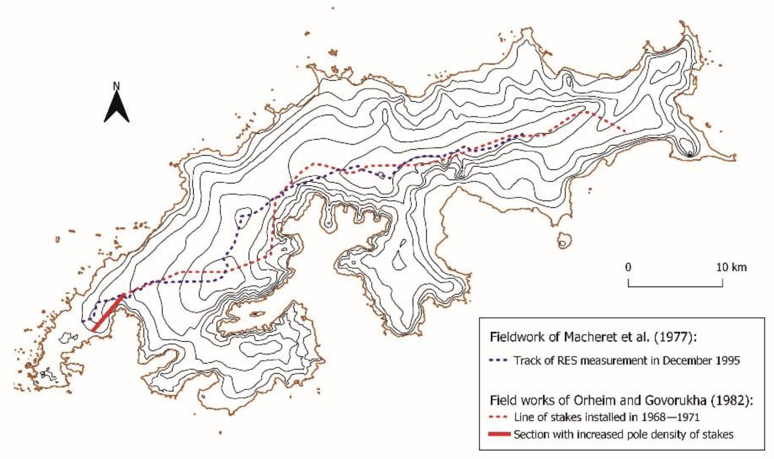
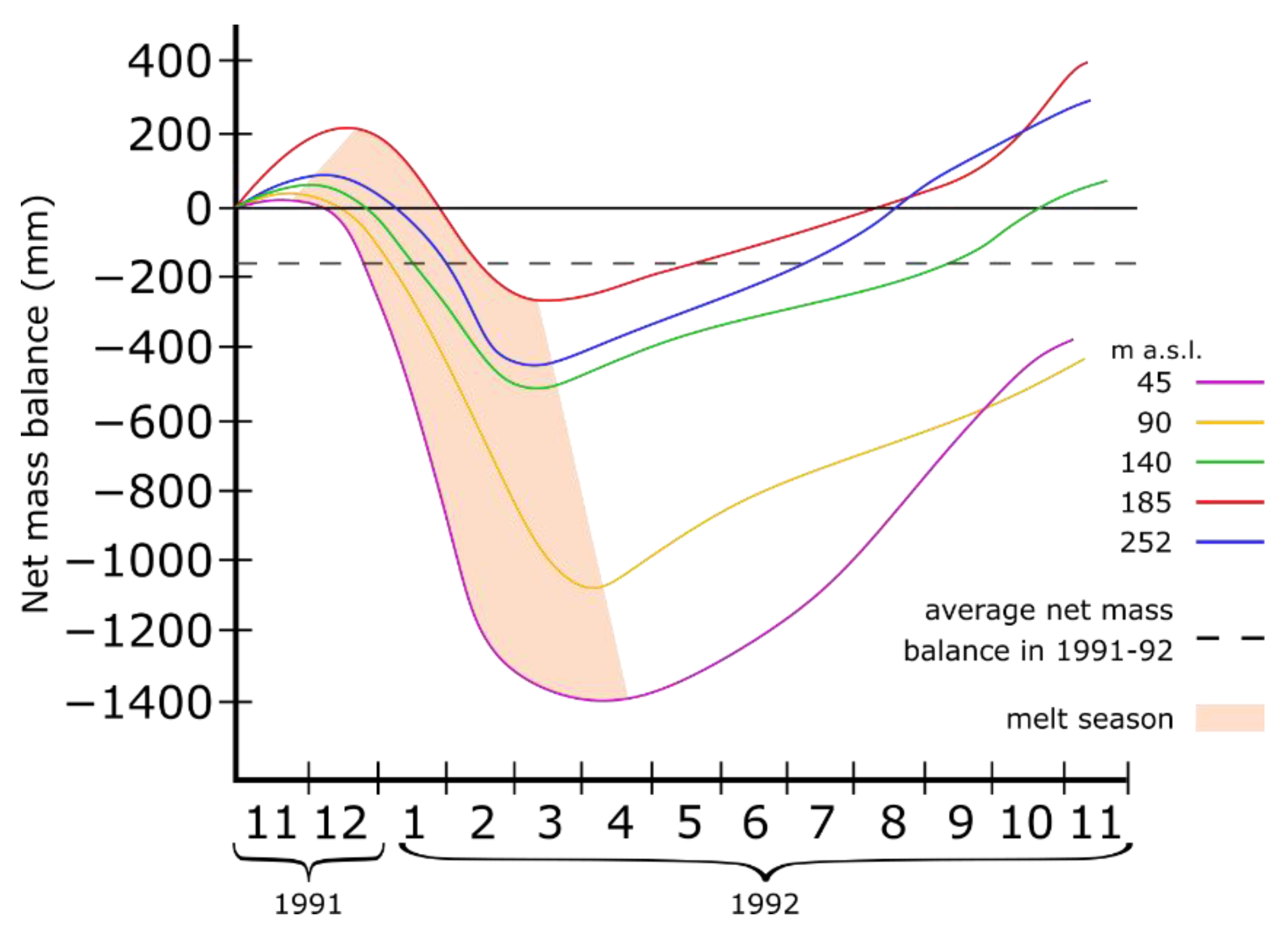
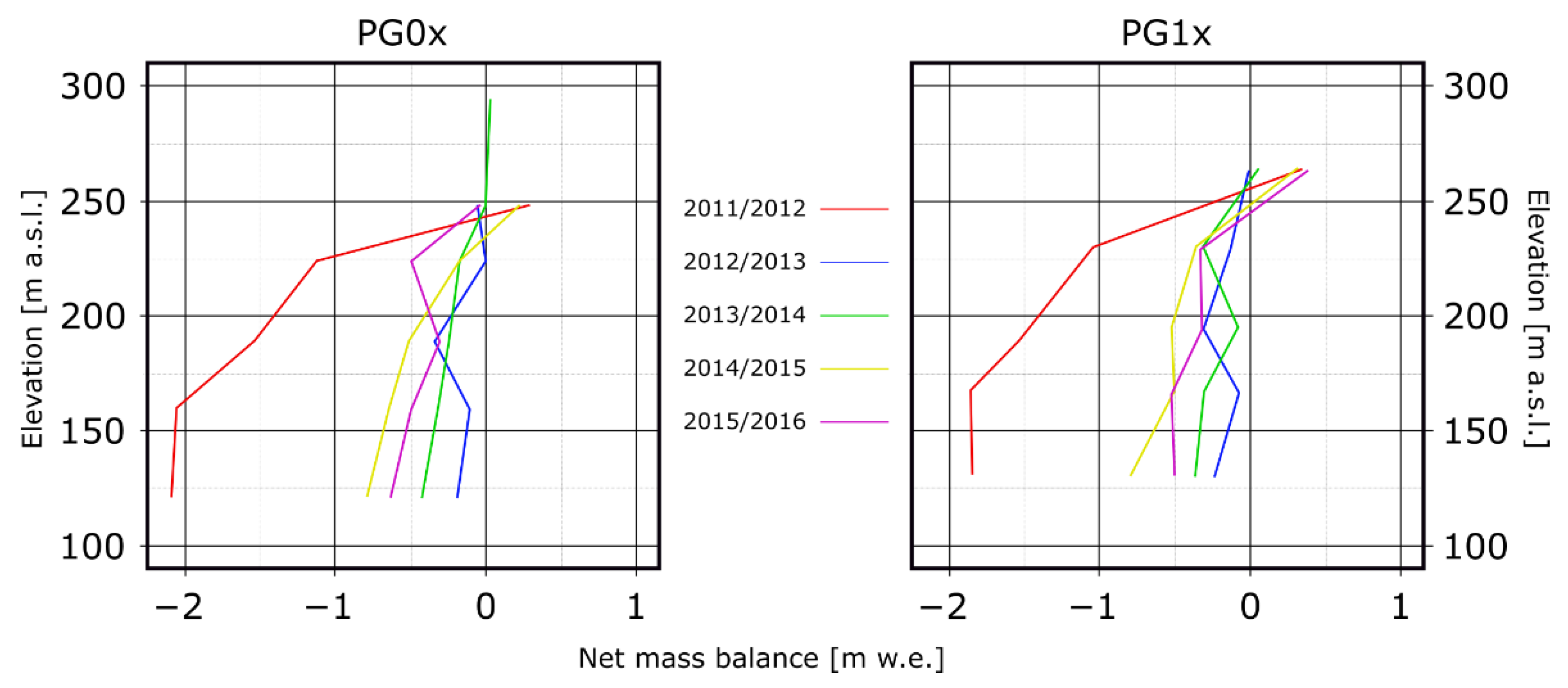
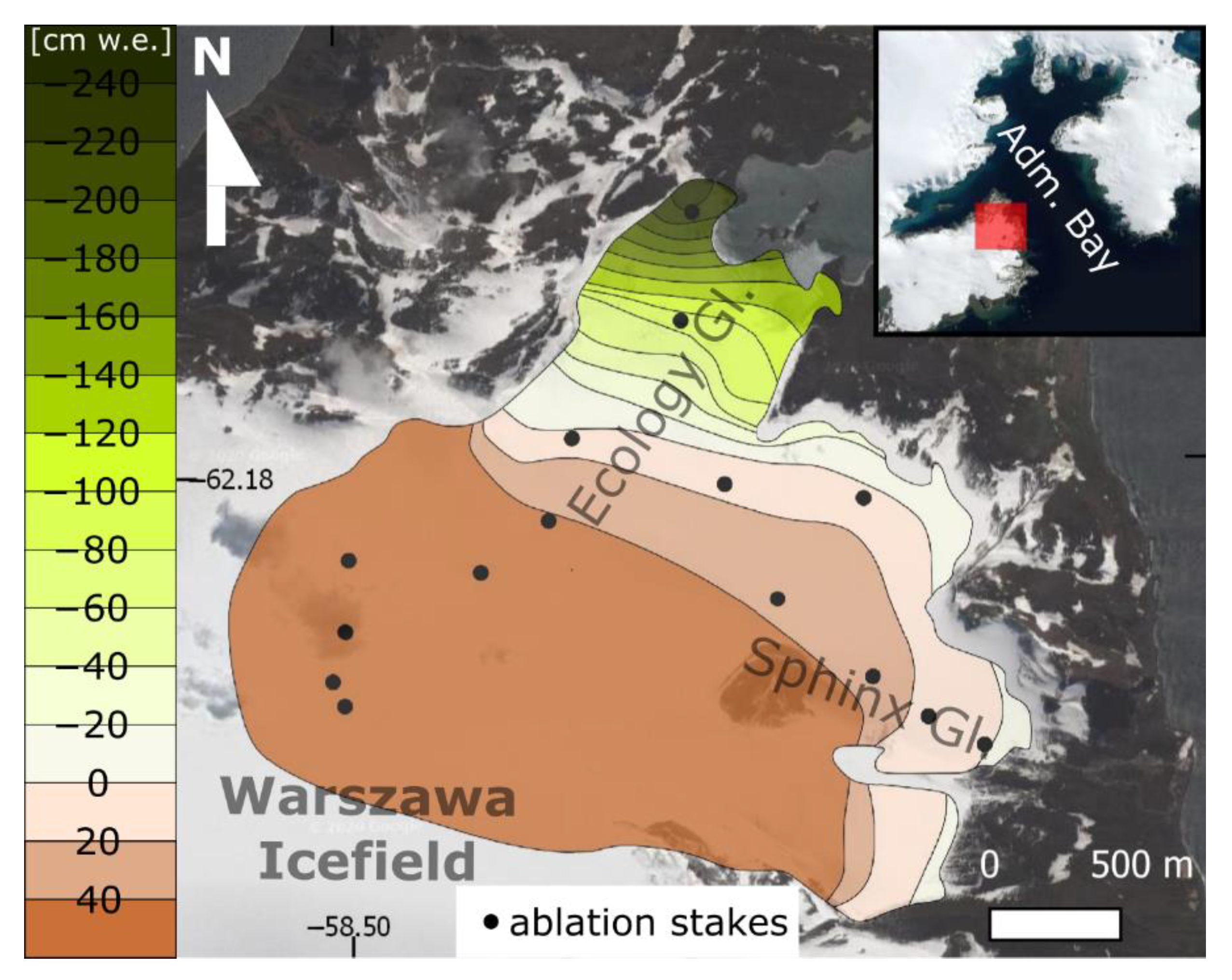
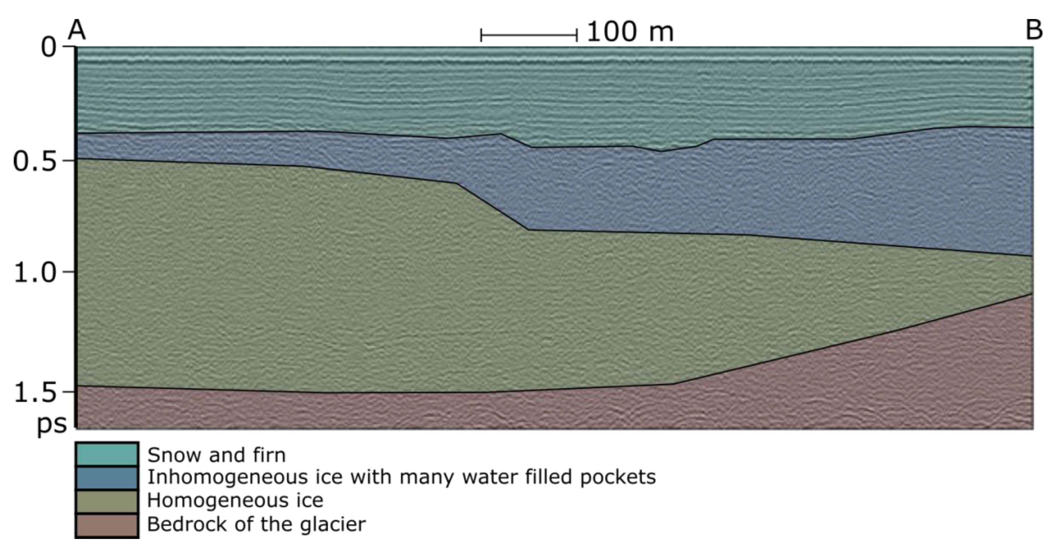
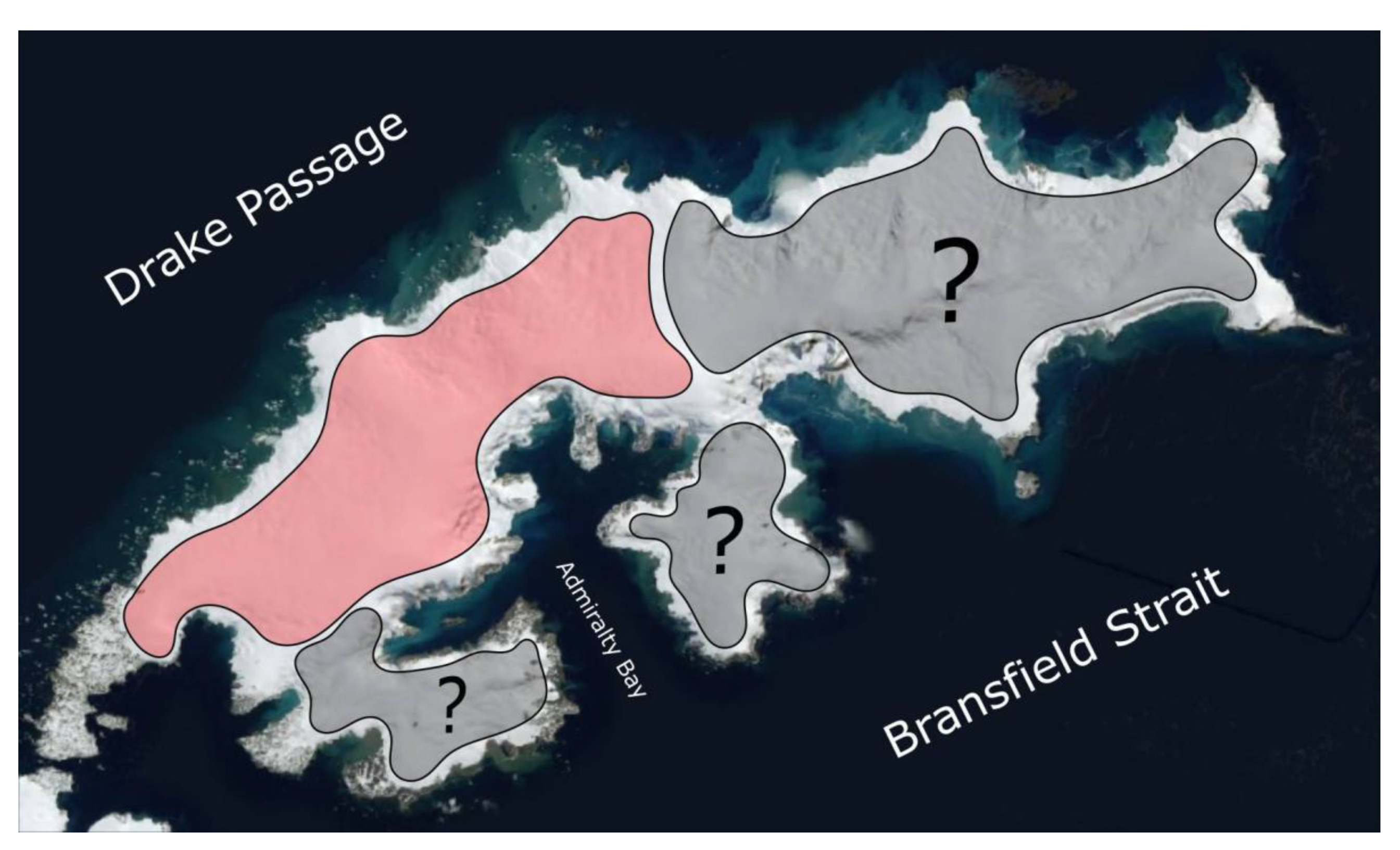
Table A1.
The research performed to date on the parameters that compose the mass balance of glaciers on KGI glaciers.
Table A1.
The research performed to date on the parameters that compose the mass balance of glaciers on KGI glaciers.
| Location | Measuring Period or Date | Elevation (m a.s.l.) | Accumulation | Ablation | Mass Balance | References |
|---|---|---|---|---|---|---|
| [mm w.e. a−1] | ||||||
| KGI Ice Cap (Arctowski Icefield, Central and East Part) | 1957/1958–1970-71 | 240 | − | − | 500−700 | [26] |
| Arctowski Icefield | Coring from 1985–1992, 18 m depth | 380 | 1175 | − | − | [37] |
| Arctowski Icefield | Coring from 1985–1992, 18 m depth | 510 | 1630 | − | − | [37] |
| Arctowski Icefield | Coring from 1985–1992, 18 m depth | 610 | 2040 | − | − | [37] |
| Arctowski Icefield | Coring from 1985–1992, 18 m depth | 702 | 2480 | − | − | [37] |
| Arctowski Icefield | 2 December 1997–12 January 1998 | − | − | 260 | − | [34] |
| Arctowski Icefield | 2 December 1997–12 January 1998 | 85 | − | 383 | − | [32] |
| Arctowski Icefield | Decemebr 1999–March 2000 | 255 | − | 1150 | − | [34] |
| Arctowski Icefield | 2007/2008 | 390 | 3680 | − | − | [43] |
| Arctowski Icefield | 2007/2008 | 417 | 4120 | − | − | [43] |
| Arctowski Icefield | 2007/2008 | 488 | 3756 | − | − | [43] |
| Arctowski Icefield | 2007/2008 | 489 | 3735 | − | − | [43] |
| Arctowski Icefield | 2007/2008 | 552 | 3976 | − | − | [43] |
| Arctowski Icefield | 2007/2008 | 568 | 4839 | − | − | [43] |
| Arctowski Icefield | 2007/2008 | 612 | 4634 | − | − | [43] |
| Arctowski Icefield | 2007/2008 | 622 | 3994 | − | − | [43] |
| Arctowski Icefield | 2007/2008 | 631 | 4388 | − | − | [43] |
| Arctowski Icefield | 2007/2008 | 639 | 5047 | − | − | [43] |
| Arctowski Icefield | 2008/2009 | 390 | 3184 | − | − | [43] |
| Arctowski Icefield | 2008/2009 | 417 | 1639 | − | − | [43] |
| Arctowski Icefield | 2008/2009 | 488 | 1854 | − | − | [43] |
| Arctowski Icefield | 2008/2009 | 489 | 1574 | − | − | [43] |
| Arctowski Icefield | 2008/2009 | 552 | − | − | − | [43] |
| Arctowski Icefield | 2008/2009 | 568 | 2244 | − | − | [43] |
| Arctowski Icefield | 2008/2009 | 612 | 2611 | − | − | [43] |
| Arctowski Icefield | 2008/2009 | 622 | − | − | − | [43] |
| Arctowski Icefield | 2008/2009 | 631 | 2133 | − | − | [43] |
| Arctowski Icefield | 2008/2009 | 639 | 2590 | − | − | [43] |
| Central part | 2007/2008 | 428 | 3891 | − | − | [43] |
| Central part | 2007/2008 | 434 | 3942 | − | − | [43] |
| Central part | 2007/2008 | 454 | 3361 | − | − | [43] |
| Central part | 2007/2008 | 515 | 4178 | − | − | [43] |
| Central part | 2007/2008 | 520 | 4321 | − | − | [43] |
| Central part | 2007/2008 | 538 | 3639 | − | − | [43] |
| Central part | 2007/2008 | 561 | 4180 | − | − | [43] |
| Central part | 2007/2008 | 593 | 4950 | − | − | [43] |
| Central part | 2007/2008 | 594 | 4157 | − | − | [43] |
| Central part | 2007/2008 | 627 | 4574 | − | − | [43] |
| Central part | 2007/2008 | 652 | 4288 | − | − | [43] |
| Central part | 2007/2008 | 658 | 4911 | − | − | [43] |
| Central part | 2007/2008 | 691 | 4279 | − | − | [43] |
| Bellingshausen Dome | Coring in 1991, 80.2 m depth | 240 | 700 | − | − | [39] |
| Bellingshausen Dome | 1971–1991 | − | − | − | −4.5 | [37,52] |
| Bellingshausen Dome | 1971–1972 | − | − | − | −68.1 | [52] |
| Bellingshausen Dome | 1972–1973 | − | − | − | −59.3 | [52] |
| Bellingshausen Dome | 1973–1974 | − | − | − | −229.1 | [52] |
| Bellingshausen Dome | 1974–1975 | − | − | − | −35.2 | [52] |
| Bellingshausen Dome | 1975–1976 | − | − | − | −36.8 | [52] |
| Bellingshausen Dome | 1976–1977 | − | − | − | −8.5 | [52] |
| Bellingshausen Dome | 1977–1978 | − | − | − | 30.1 | [52] |
| Bellingshausen Dome | 1978–1979 | − | − | − | −175 | [52] |
| Bellingshausen Dome | 1979–1980 | − | − | − | 62.9 | [52] |
| Bellingshausen Dome | 1980–1981 | − | − | − | −4.1 | [52] |
| Bellingshausen Dome | 1981–1982 | − | − | − | −68.1 | [52] |
| Bellingshausen Dome | 1982–1983 | − | − | − | −160.7 | [52] |
| Bellingshausen Dome | 1983–1984 | − | − | − | −157.7 | [52] |
| Bellingshausen Dome | 1984–1985 | − | − | − | 126.2 | [52] |
| Bellingshausen Dome | 1985–1986 | − | − | − | 189.8 | [52] |
| Bellingshausen Dome | 1986–1987 | − | − | − | 56.2 | [52] |
| Bellingshausen Dome | 1987–1988 | − | − | − | −189.2 | [52] |
| Bellingshausen Dome | 1988–1989 | − | − | − | 33.1 | [52] |
| Bellingshausen Dome | 1989–1990 | − | − | − | 93.3 | [52] |
| Bellingshausen Dome | 1990–1991 | − | − | − | 467.9 | [52] |
| Bellingshausen Dome | 1991–1992 | − | − | − | 163 | [37] |
| Bellingshausen Dome | November 1991–November 1992 | 45 | − | − | 1430 | [37] |
| Bellingshausen Dome | November 1991–November 1992 | 90 | − | − | 1100 | [37] |
| Bellingshausen Dome | November 1991–November 1992 | 140 | − | − | 550 | [37] |
| Bellingshausen Dome | November 1991–November 1992 | 185 | − | − | 520 | [37] |
| Bellingshausen Dome | November 1991–November 1992 | 252 | − | − | 410 | [37] |
| Bellingshausen Dome | Coring from 1985–1992, 18 m depth | 110 | 650 * | − | − | [37] |
| Bellingshausen Dome | Coring from 1985–1992, 18 m depth | 150 | 540 * | − | − | [37] |
| Bellingshausen Dome | Coring from 1985–1992, 18 m depth | 185 | 970 * | − | − | [37] |
| Bellingshausen Dome | Coring from 1985–1992, 18 m depth | 252 | 530 * | − | − | [37] |
| Bellingshausen Dome | December 1995–March 1996 | 35 | − | 750 | − | [34] |
| Bellingshausen Dome | December 1997–March 1998 | 85 | − | 1100 | − | [34] |
| Bellingshausen Dome | 2007–2012 | − | 752.8 | −900 | −147.3 | [53] |
| Bellingshausen Dome | 2007/2008 | − | 654.4 | −736 | −81.6 | [53] |
| Bellingshausen Dome | 2008/2009 | − | 565.2 | −1259 | −693.8 | [53] |
| Bellingshausen Dome | 2009/2010 | − | 800.6 | −426 | 374.6 | [53] |
| Bellingshausen Dome | 2010/2011 | − | 1034,4 | −941 | 93.4 | [53] |
| Bellingshausen Dome | 2011/2012 | − | 709.5 | −1139 | −429 | [53] |
| Stenhouse Glacier | 1957/1958 | − | − | − | −50 | [48] |
| Stenhouse Glacier | 1958/1959 | − | − | − | −50 | [29] |
| Stenhouse Glacier | Summer season 1959/1960 | − | − | 1310 | − | [29] |
| Flagstaff Glacier | Summer season 1957/1958 | 130−230 | − | 750 | − | [28] |
| Flagstaff Glacier | 3 February–21 April 1959 | − | − | 544 | − | [29] |
| Fourcade Glacier | 2010/2011 | − | − | − | −134 | [46] |
| Fourcade Glacier | 2012/2013 | − | − | − | −201 | [46] |
| Fourcade Glacier | 2013/2014 | − | − | − | −97 | [46] |
| Fourcade Glacier | 2014/2015 | − | − | − | −196 | [46] |
| Lange Glacier | 73-year average, coring in 1995/96, | 690 | 590 | − | − | [40] |
| Ecology Glacier | December 1990–January 1991 | 100 | − | 735 ** | − | [31] |
| Ecology and Sphinx glacier system | 2012–2013 | − | − | − | 178 | [35] |
* winter accumulation. ** ablation for period 17 December 1990–16 January 1991.
Table A2.
The collated results of ELA and FLA fluctuation observations collected on KGI glaciers. * winter accumulation.
Table A2.
The collated results of ELA and FLA fluctuation observations collected on KGI glaciers. * winter accumulation.
| Balance Year | Location | ELA/FLA [m a.s.l.] | References |
|---|---|---|---|
| 1957 | Flagstaff Glacier | 198 | [29] |
| 1959 | Flagstaff Glacier | 130 | [29] |
| 1960 | Admiralty Bay | 300 | [29] |
| 1969/70 | Bellingshausen Dome | 140 | [26] |
| 1970/71 | Bellingshausen Dome | 170 | [26] |
| 1972/73 | Stenhouse Glacier | <100 | [48] |
| 1973/74 | Stenhouse Glacier | <100 | [48] |
| 1985/86 | Bellingshausen Dome | 150 | [50,51] |
| 1988 | Admiralty Bay | 350 | [22] |
| 1985–1989 | South Shetland Islands | <100 | [120] |
| 1991/92 | Bellingshausen Dome | 140 | [37] |
| 1991/92 | Ecology Glacier | about 100 | [31] |
| 1991/92 | Bellingshausen Dome | 160 | [58] |
| 1992/93 | Bellingshausen Dome | 200 | [58] |
| 1993/94 | Bellingshausen Dome | 200 | [58] |
| 1993 | Admiralty Bay | 300–350 * | [56] |
| 1994–1995 | Admiralty Bay | 450 | [22] |
| 1995/96 | Bellingshausen Dome | 200 | [58] |
| 1996/97 | Bellingshausen Dome | 250−270 | [58] |
| 1996/97 | KGI | 250 | [58] |
| 1997/98 | Bellingshausen Dome | 180−200 | [58] |
| 1998/99 | Bellingshausen Dome | 200−220 | [58] |
| 2006/07 | Admiralty Bay | 290 | [55] |
| 2007/08 | Bellingshausen Dome | 225 | [53] |
| 2008/09 | Bellingshausen Dome | 225 | [53] |
| 2009/10 | Bellingshausen Dome | about 40 | [53] |
| 2010/11 | Bellingshausen Dome | 180 | [53] |
| 2011/12 | Bellingshausen Dome | 220 | [53] |
| 2012/13 | Ecology and Sphinx glacier system | 156 | [35] |
| 2010–2015 | Fourcade Glacier | 260 +/− 20 | [17] |
| 2010–2015 | KGI | 330 +/− 100 | [54] |
| 1991–1999 | South Shetland Islands | 165–250 | [121] |
References
- Cuffey, K.M.; Paterson, W.S.B. The Physics of Glaciers; Academic Press: Cambridge, MA, USA, 2010; p. 54. [Google Scholar]
- Meier, M.F. Glaciers and climate. In Polar Record; Wright, H.E., Frey, D.G., Eds.; Princeton University Press: Princeton, NJ, USA, 1965; Volume 22, pp. 795–805. [Google Scholar]
- Oerlemans, J. Glaciers and Climate Change; CRC Press: Boca Raton, FL, USA, 2001; p. 54. [Google Scholar]
- Dyurgerov, M.B.; Meier, M.F. Glaciers and the Changing Earth system: A 2004 Snapshot; Institute of Arctic and Alpine Research: Boulder, CO, USA, 2005; p. 58. [Google Scholar]
- Der Veen, C.J. Fundamentals of Glacier Dynamics; CRC Press: Boca Raton, FL, USA, 2013; p. 58. [Google Scholar]
- Benn, D.; Evans, D.J.A. Glaciers and Glaciation; Routledge: Abingdon-on-Thames, UK, 2014; p. 58. [Google Scholar]
- Oliva, M.; Navarro, F.; Hrbáček, F.; Hernandéz, A.; Nývlt, D.; Pereira, P.; Ruiz-Fernandéz, J.; Trigo, R. Recent regional climate cooling on the Antarctic Peninsula and associated impacts on the cryosphere. Sci. Total Environ. 2017, 580, 210–223. [Google Scholar] [CrossRef]
- Jania, J. Glacjologia: Nauka o lodowcach. Wydaw. Naukowe PWN 1997, 58, 359. [Google Scholar]
- Kaser, G.; Fountain, A.; Jansson, P.; Erich, H.; Mathias, K. A Manual for Monitoring the Mass Balance of Mountain Glaciers; Unesco: Paris, France, 2003; p. 58. [Google Scholar]
- Bamber, J.L.; Payne, A.J. Mass Balance of the Cryosphere: Observations and Modelling of Contemporary and Future Changes; Cambridge University Press: Cambridge, UK, 2004; p. 662. [Google Scholar]
- Bamber, J.L.; Rivera, A. A review of remote sensing methods for glacier mass balance determination. Glob. Planet. Chang. 2007, 59, 138–148. [Google Scholar] [CrossRef]
- Watson, C.S.; Quincey, D. Glacier Movement. Geomorphol. Tech. 2015, 59, 138–148. [Google Scholar]
- Bogorodsky, V.V.; Bentley, C.R.; Gudmandsen, P.E. Radioglaciology; Springer: Berlin/Heidelberg, Germany, 1985. [Google Scholar]
- Grabiec, M. Stan i Współczesne Zmiany Systemów Lodowcowych Południowego Spitsbergenu w Świetle Badan Metodami Radarowymi; Wydawnictwo Uniwersytetu Śląskiego: Katowice, Poland, 2017; p. 58. [Google Scholar]
- Miers, J. John Miers account of the discovery of the South Shetland Islands. Polar Rec. 1950, 5, 565–575. [Google Scholar]
- Jones, A.G.E. Captain William Smith and the discovery of new South Shetland. Geogr. J. 1975, 5, 445–461. [Google Scholar] [CrossRef]
- Falk, U.; López, D.A.; Silva-Busso, A. Multi-year analysis of distributed glacier mass balance modelling and equilibrium line altitude on King George Island, Antarctic Peninsula. Cryosphere 2018, 12, 1211–1232. [Google Scholar] [CrossRef] [Green Version]
- Montone, R.C.; Alvarez, C.E.; Bícego, M.C.; Braga, E.S.; Brito, T.A.S.; Campos, L.S.; Fontes, R.F.C.; Castro, B.M.; Corbisier, T.N.; Evangelista, H.; et al. Environmental assessment of admiralty bay, King George Island, Antarctica. In Environment: Science and Policy for Sustainable Development; Springer: Berlin/Heidelberg, Germany, 2013; Volume 51, pp. 157–175. [Google Scholar]
- Oerlemans, J.; Fortuin, J.P.F. Sensitivity of glaciers and small ice caps to greenhouse warming. Science 1992, 258, 115–117. [Google Scholar] [CrossRef]
- Kejna, M.; Araźny, A.; Sobota, I. Climatic change on King George Island in the years 1948–2011. Pol. Polar Res. 2013, 34, 213–235. [Google Scholar] [CrossRef]
- Plenzler, J.; Budzik, T.; Puczko, D.; Bialik, R. Climatic conditions at Arctowski Station (King George Island, West Antarctica) in 2013–2017 against the background of observed regional changes. Pol. Polar Res. 2019, 40, 1–27. [Google Scholar]
- Simões, J.C.; Bremer, U.F.; Aquino, F.E.; Ferron, F.A. Morphology and variations of glacial drainage basins in the King George Island ice field, Antarctica. Ann. Glaciol. 1999, 29, 220–224. [Google Scholar] [CrossRef] [Green Version]
- Osmanoğlu, B.; Braun, M.; Hock, R.; Navarro, F.J. Surface velocity and ice discharge of the ice cap on King George Island, Antarctica. Ann. Glaciol. 2013, 54, 111–119. [Google Scholar] [CrossRef] [Green Version]
- Orheim, O. A 200-Year Record of Glacier Mass Balance at Deception Island, Southwest Atlantic Ocean, and Its Bearing on Models of Global Climatic Change; Princeton University Press: Princeton, NJ, USA, 1972; p. 4. [Google Scholar]
- Orheim, O.; Schytt, V.; Bull, C. Glaciologica studies of past climatic variations in South Shetlands Islands. Antarct. J. USA 1972, 7, 99. [Google Scholar]
- Orheim, O.; Govorukha, L.S. Present-Day Glaciation in the South Shetland Islands. Ann. Glaciol. 1982, 3, 233–238. [Google Scholar] [CrossRef]
- Braun, M. Ablation on the Ice Cap of King George Island (Antarctica); Springer: Berlin/Heidelberg, Germany, 2001; p. 26. [Google Scholar]
- Noble, H.M. Glaciological observations at Admiralty Bay, King George Island, in 1957–1958. Br. Antarct. Surv. Bull. 1965, 5, 1–11. [Google Scholar]
- Stansbury, M.J. Glaciological observations at Admiralty Bay (Lat. 62°05′ S, Lon. 58°24′W), King George Island, South Shetland Islands, 1959–60. Falkl. Isl. Depend. Surv. Prelim. Glaciol. Rep. 1961, 4, 45. [Google Scholar]
- Bintanja, R. Glaciological and meteorological investigations on Ecology Glacier, King George Island, Antarctica (Summer 1990–1991). Circumpolar J. 1992, 7, 59–71. [Google Scholar]
- Bintanja, R. The local surface energy balance of the Ecology Glacier, King George Island, Antarctica: Measurements and modelling. Antarct. Sci. 1995, 7, 315–325. [Google Scholar] [CrossRef]
- Braun, M.; Saurer, H.; Vogt, S.; Simões, J.C.; Goßmann, H. The influence of large-scale atmospheric circulation on the surface energy balance of the King George Island ice cap. Int. J. Climatol. J. R. Meteorol. Soc. 2001, 21, 21–36. [Google Scholar] [CrossRef]
- Braun, M.; Hock, R. Spatially distributed surface energy balance and ablation modelling on the ice cap of King George Island (Antarctica). Glob. Planet. Chang. 2004, 42, 45–58. [Google Scholar] [CrossRef]
- Braun, M.; Saurer, H.; Goßmann, H. Climate, energy fluxes and ablation rates on the ice cap of King George Island. Pesqui. Antárt. Bras. 2004, 4, 87–103. [Google Scholar]
- Sobota, I.; Kejna, M.; Araźny, A. Short-term mass changes and retreat of the Ecology and Sphinx glacier system, King George Island, Antarctic Peninsula. Antarct. Sci. 2015, 27, 500–510. [Google Scholar] [CrossRef]
- Huss, M.; Dhulst, L.; Bauder, A. New long-term mass-balance series for the Swiss Alps. J. Glaciol. 2015, 61, 551–562. [Google Scholar] [CrossRef] [Green Version]
- Wen, J.; Kang, J.; Han, J.; Xie, Z.; Liu, L.; Wang, D. Glaciological studies on the King George Island ice cap, South Shetland Islands, Antarctica. Ann. Glaciol. 1998, 27, 105–109. [Google Scholar]
- Zamoruyev, V. V Results of glaciological observations at Bellingshausen station in 1968. Tr. Sov. Antarkt. Ekspeditsii 1972, 55, 135–144. [Google Scholar]
- Jiankan, H.; Zichu, X.; Fengnian, D.; Wanchang, Z. Volcanic eruptions recorded in an ice core from Collins Ice Cap, King George Island, Antarctica. Ann. Glaciol. 1999, 29, 121–125. [Google Scholar] [CrossRef] [Green Version]
- Simões, J.C.; Ferron, F.A.; Bernardo, R.T.; Aristarain, A.J.; Stiévenard, M.; Pourchet, M.; Delmas, R.J. Ice core study from the king george island, south shetlands, antarctica. Pesqui. Antárt. Bras. 2004, 4, 9–23. [Google Scholar]
- Ferron, F.A. Variações Nas Razões de Isótopos Estáveis na Neve e no Gelo da Ilha Rei George, Antártica. Master’s Thesis, IG/UFRGS, Porto Alegre, Brazil, 1999; p. 125. [Google Scholar]
- Bernardo, R.T. Conteúdo Aniônico da Neve e do Gelo da Ilha Rei George, Antartica. Master’s Thesis, em Geociências, Instituto de Gências, Universidade, Porto Alegre, Brazil, 1999; p. 100. [Google Scholar]
- Rückamp, M.; Braun, M.; Suckro, S.; Blindow, N. Observed glacial changes on the King George Island ice cap, Antarctica, in the last decade. Glob. Planet. Chang. 2011, 79, 99–109. [Google Scholar] [CrossRef]
- Marshall, G.J.; Rees, W.G.; Dowdeswell, J.A. The discrimination of glacier facies using multi-temporal ERS-1 SAR data. Sens. Environ. Appl. Remote Sens. 1995, 9, 263–269. [Google Scholar]
- Smith, L.C.; Forster, R.R.; Isacks, B.L.; Hall, D.K. Seasonal climatic forcing of alpine glaciers revealed with orbital synthetic aperture radar. J. Glaciol. 1997, 43, 480–488. [Google Scholar] [CrossRef] [Green Version]
- Falk, U.; Sala, H. Winter melt conditions of the inland ice cap on King George Island, Antarctic Peninsula. Erdkunde 2015, 38, 341–363. [Google Scholar] [CrossRef]
- De Robin, G.Q.; Adie, R.J. The ice cover. Antarct. Res. 1964, 8, 100–117. [Google Scholar]
- Curl, J.E. A Glacial History of the South Shetland Islands, Antarctica; Wright, H.E., Frey, D.G., Eds.; Princeton University Press: Princeton, NJ, USA, 1980; p. 5. [Google Scholar]
- Macheret, Y.Y.; Moskalevsky, M.Y.; Simões, J.C.; Ladouch, L. Study of King George Island ice cap, South Shetland Islands, Antarctica using radio-echo sounding and spot, ERS-1 SAR satellite images. In Proceedings of the European Space Agency, (Special Publication) ESA SP., PAN, Vina del Mar, Chile, 25–29 November 1997; Volume 8, pp. 249–253. [Google Scholar]
- Ren, J. Development conditions and mass balance in the glaciers nearby the Great Wall Station, Antarctica. Collect. Antarct. Sci. Explor. 1988, 9, 247–255. [Google Scholar]
- Ren, J.; Dahe, Q.; Petit, J.R.; Jouzel, J.; Wenti, W.; Chen, L.; Xiaojun, W.; Songlin, Q.; Xiaoxiang, W. Glaciological studies on Nelson Island, South Shetland Islands, Antarctica. J. Glaciol. 1995, 41, 408–412. [Google Scholar]
- Wen, J.; Kang, J.; Xie, Z.; Han, J.; Lluberas, A. Climate, mass balance and glacial changes on small dome of Collins Ice Cap, King George Island, Antarctica. Antarct. Res. 1994, 5, 52–61. [Google Scholar]
- Mavlyudov, R. Ice mass balance of the Bellingshausen ice cap in 2007–2012 (King George Island, South Shetland Islands, Antarctica). Ice Snow 2014, 54, 27–34. [Google Scholar] [CrossRef] [Green Version]
- Falk, U.; Lopez, D.; Silva-Busso, A. Sensitivity of Glacier Mass Balance and Equilibrium Line Altitude to Climatic Change on King George Island, Antarctic Peninsula; British Antarctic Survey Bulletin; Wright, H.E., Frey, D.G., Eds.; Princeton University Press: Princeton, NJ, USA, 2017; Volume 19, p. 9409. [Google Scholar]
- Pudełko, R.; Angiel, P.; Potocki, M.; Jędrejek, A.; Kozak, M. Fluctuation of glacial retreat rates in the eastern part of Warszawa Icefield, King George Island, Antarctica, 1979–2018. Remote Sens. 2018, 10, 892. [Google Scholar] [CrossRef] [Green Version]
- Simões, J.C.; Bremer, U.F. Investigations of King George Island ice cover using ERS-1/SAR and SPOT imagery. Rev. Selper 1995, 11, 56–60. [Google Scholar]
- Braun, M.; Rau, F. Using a multi-year data archive of ERS SAR imagery for the monitoring of firn line positions and ablation patterns on the King George Island ice cap (Antarctica). EARSeL eProc. 2000, 1, 281–291. [Google Scholar]
- Braun, M.; Rau, F.; Saurer, H.; Gobmann, H. Development of radar glacier zones on the King George Island ice cap, Antarctica, during austral summer 1996/97 as observed in ERS-2 SAR data. Ann. Glaciol. 2000, 31, 357–363. [Google Scholar] [CrossRef] [Green Version]
- Jania, J.; Grabiec, M.; Kolondra, L.; Puczko, D.; Głowacki, P.; Migała, K.; Budzik, T. Wyniki najnowszych studiów nad współczesną ewolucją lodowców Svalbardu (ze szczególnym uwzględnieniem południowego Spitsbergenu). w: Guterch, A.(red.). In Proceedings of the Struktura, Ewolucja i Dynamika Litosfery, Kriosfery i Biosfery w Europejskim Sektorze Arktyki oraz w Antarktyce (2004–2007), Warszawa, Poland, 29–30 October 2007; Volume 34, pp. 29–30. [Google Scholar]
- Silva, A.B.; Arigony-Neto, J.; Braun, M.H.; Espinoza, J.M.A.; Costi, J.; Jaña, R. Spatial and temporal analysis of changes in the glaciers of the Antarctic Peninsula. Glob. Planet. Chang. 2020, 184, 103079. [Google Scholar] [CrossRef]
- Cook, A.J.; Fox, A.J.; Vaughan, D.G.; Ferrigno, J.G. Retreating glacier fronts on the Antarctic Peninsula over the past half-century. Science 2005, 308, 541–544. [Google Scholar] [CrossRef] [Green Version]
- Mosley-Thompson, E.; Paskievitch, J.F.; Gow, A.J.; Thompson, L.G. Late 20th century increase in South Pole snow accumulation. J. Geophys. Res. Atmos. 1999, 104, 3877–3886. [Google Scholar] [CrossRef]
- Shepherd, A.; Wingham, D.; Payne, T.; Skvarca, P. Larsen ice shelf has progressively thinned. Science 2003, 302, 856–859. [Google Scholar] [CrossRef] [Green Version]
- Stone, J.O.; Balco, G.A.; Sugden, D.E.; Caffee, M.W.; Sass, L.C.; Cowdery, S.G.; Siddoway, C. Holocene deglaciation of Marie Byrd land, west Antarctica. Science 2003, 299, 99–102. [Google Scholar] [CrossRef] [PubMed] [Green Version]
- Calvet, J.; Corbera, J.; Furdada, G. Variación del frente glaciar en Bahia Sur y Punta Siddons entre 1956 y 1991, Isla Livingston, Islas Shetland del Sur. Simposios: III Congreso Geológico de España y VIII Congreso Latinoamericano de Geología; University of Salamanca: Salamanca, Spain, 1992; Volume 3, pp. 283–292. [Google Scholar]
- Park, B.-K.; Chang, S.-K.; Yoon, H.I.; Chung, H. Recent retreat of ice cliffs, King George Island, South Shetland Islands, Antarctic Peninsula. Ann. Glaciol. 1998, 27, 633–635. [Google Scholar] [CrossRef] [Green Version]
- Simões, J.C.; Dani, N.; Bremer, U.F.; Aquino, F.E.; Arigony Neto, J. Small cirque glaciers retreat on Keller Peninsula, Admiralty Bay, King George Island, Antarctica. Braz. Antarct. Res. 2004, 4, 49–56. [Google Scholar]
- Pętlicki, M.; Sziło, J.; MacDonell, S.; Vivero, S.; Bialik, R. Recent deceleration of the ice elevation change of Ecology Glacier (King George Island, Antarctica). Remote Sens. 2017, 9, 520. [Google Scholar] [CrossRef] [Green Version]
- Sziło, J.; Bialik, R. Recession and ice surface elevation changes of Baranowski Glacier and its impact on proglacial relief (King George Island, West Antarctica). Geosciences 2018, 8, 355. [Google Scholar] [CrossRef] [Green Version]
- Simões, C.L.; da Rosa, K.K.; Czapela, F.F.; Vieira, R.; Simões, J.C. Collins Glacier retreat process and regional climatic variations, King George Island, Antarctica. Geogr. Rev. 2015, 105, 462–471. [Google Scholar] [CrossRef]
- Da Rosa, K.K.; Vieira, R.; Fernandez, G.; Mendes, C.W., Jr.; Arigony-Neto, J.; Velho, L.F.; Simões, J.C. Recent changes in the Wanda Glacier, King George Island, Antarctica. Pesqui. Geocienc. 2015, 8, 575. [Google Scholar] [CrossRef]
- Braun, M.; Simões, J.C.; Vogt, S.; Bremer, U.F.; Blindow, N.; Pfender, M.; Saurer, H.; Aquino, F.E.; Ferron, F.A. An improved topographic database for King George Island: Compilation, application and outlook. Antarct. Sci. 2001, 13, 41–52. [Google Scholar] [CrossRef] [Green Version]
- Macheret, Y.Y.; Moskalevsky, M.Y. Study of Lange Glacier on King George Island, Antarctica. Ann. Glaciol. 1999, 29, 202–206. [Google Scholar] [CrossRef] [Green Version]
- Braun, M.; Gossmann, H. Glacial Changes in the Areas of Admiralty Bay and Potter Cove, King George Island, Maritime Antarctica. In Geoecology of Antarctic Ice-Free Coastal Landscapes; Springer: Berlin/Heidelberg, Germany, 2002; pp. 75–89. [Google Scholar]
- Rückamp, M.; Blindow, N.; Suckro, S.; Braun, M.; Humbert, A. Dynamics of the ice cap on King George Island, Antarctica: Field measurements and numerical simulations. Ann. Glaciol. 2010, 51, 80–90. [Google Scholar] [CrossRef] [Green Version]
- Van Der Veen, C.J. Tidewater calving. J. Glaciol. 1996, 42, 375–385. [Google Scholar] [CrossRef] [Green Version]
- Kim, Y.K.; Baek, W.D. Bathymetric and topographic measurements around King Sejong Station, King George Island, Antarctica (II). In The Studies on Natural Environments and Resource of Antarctica; Korea Ocean Research and Development Institute (KORDI): Seoul, Korea, 1995; pp. 825–846. [Google Scholar]
- Instituto Hidrográfico de la Armada de Chile. Caleta Potter; Instituto Hidrográfico de la Armada de Chile: Playa Ancha, Chile, 1980. [Google Scholar]
- Peel, D.A.; Mulvaney, R.; Davison, B.M. Stable-isotope/air-temperature relationships in ice cores from Dolleman Island and the Palmer Land plateau, Antarctic Peninsula. Ann. Glaciol. 1988, 10, 130–136. [Google Scholar] [CrossRef]
- Muser, D. Der Gletscherrückzug auf King George Island, South Shetland Islands Zwischen 1956 und 1992. Eine Digitale Auswertung von Karten, Luftbildern und Satellitendaten. Unpublished Thesis, Albert-Ludwigs-Universität, Freiburg, Germany, 1995. [Google Scholar]
- Warren, C.R. Iceberg calving and the glacioclimatic record. Prog. Phys. Geogr. 1992, 16, 253–282. [Google Scholar] [CrossRef]
- Furmańczyk, K.; Marsz, A. South Shetland Islands, King George Island, Admiralty Bay, Topographic Map 1:25,000 Scale; Printed OP; Institute of Geography, University of Gdansk: Gdansk, Poland, 1980; pp. 183–185. [Google Scholar]
- Ferron, F.A.; Simões, J.C.; Aquino, F.E.; Setzer, A.W. Air temperature time series for King George Island, Antarctica. Pesqui. Antárt. Bras. 2004, 4, 155–169. [Google Scholar]
- Arigony-Neto, J. Determinação e Interpretação de Características Glaciológicas e Geográficas com Sistema de Informações Geográficas na Área Antártica Especialmente Gerenciada baía do Almirantado, ilha Rei George, Antártica. Unpublished Master’s Thesis, Universidade Federal do, Porto Alegre, Brazil, 2001. [Google Scholar]
- Bremer, U.F.; Arigony Neto, J.; Simões, J.C. Teledetecção de mudanças nas bacias de drenagem do gelo da ilha Rei George, Shetlands do Sul, Antártica, entre 1956 e 2000. Pesqui. Antárt. Bras. 2004, 4, 37–48. [Google Scholar]
- Francelino, M.R.; Fernandes Filho, E.I.; Schaefer, C.E.; Rezende, S.B. Fotografias Aéreas Não-Convencionais: Uma Alternativa de Monitoramento Ambiental na Antártica Marítima; Federal University of Viçosa: Viçosa, Brazil, 2003. [Google Scholar]
- Blindow, N.; Suckro, S.K.; Rückamp, M.; Braun, M.; Schindler, M.; Breuer, B.; Saurer, H.; Simões, J.C.; Lange, M.A. Geometry and thermal regime of the King George Island ice cap, Antarctica, from GPR and GPS. Ann. Glaciol. 2010, 51, 103–109. [Google Scholar] [CrossRef] [Green Version]
- Turner, J.; Lu, H.; White, I.; King, J.C.; Phillips, T.; Hosking, J.S.; Bracegirdle, T.J.; Marshall, G.J.; Mulvaney, R.; Deb, P. Absence of 21st century warming on Antarctic Peninsula consistent with natural variability. Nature 2016, 535, 411–415. [Google Scholar] [CrossRef] [PubMed] [Green Version]
- Barsch, D.; Blümel, W.-D. Untersuchungen zum Periglazial auf der König-Georg-Insel, Südshetlandinseln/Antarktika: Deutsche physiogeographische Forschungen in der Antarktis; Bericht über die Kampagne 1983/84. Ber. Polarforsch. Rep. Polar Res. 1985, 24, 75. [Google Scholar]
- Rakusa-Suszczewski, S. The Maritime Antarctic Coastal Ecosystem of Admiralty Bay; Department of Antarctic Biology, Polish Academy of Sciences: Warsaw, Poland, 1993; Volume 216, pp. 293–294. [Google Scholar]
- Meredith, M.P.; King, J.C. Rapid climate change in the ocean west of the Antarctic Peninsula during the second half of the 20th century. Geophys. Res. Lett. 2005, 32. [Google Scholar] [CrossRef]
- Oerlemans, J.; Nick, F.M. A minimal model of a tidewater glacier. Ann. Glaciol. 2005, 42, 1–6. [Google Scholar] [CrossRef] [Green Version]
- Rakusa-Suszczewski, S. King George Island? South Shetland Islands, Maritime Antarctic. In Geoecology of Antarctic Ice-Free Coastal Landscapes; Springer: Berlin/Heidelberg, Germany, 2002; pp. 23–39. [Google Scholar]
- Fieber, K.D.; Mills, J.P.; Miller, P.E.; Clarke, L.; Ireland, L.; Fox, A.J. Rigorous 3D change determination in Antarctic Peninsula glaciers from stereo WorldView-2 and archival aerial imagery. Remote Sens. Environ. 2018, 205, 18–31. [Google Scholar] [CrossRef]
- Nakamura, K.; Doi, K.; Shibuya, K. Estimation of seasonal changes in the flow of Shirase Glacier using JERS-1/SAR image correlation. Polar Sci. 2007, 1, 73–83. [Google Scholar] [CrossRef] [Green Version]
- Strozzi, T.; Kouraev, A.; Wiesmann, A.; Wegmüller, U.; Sharov, A.; Werner, C. Estimation of Arctic glacier motion with satellite L-band SAR data. Remote Sens. Environ. 2008, 112, 636–645. [Google Scholar] [CrossRef]
- Dowdeswell, J.A.; Unwin, B.; Nuttall, A.-M.; Wingham, D.J. Velocity structure, flow instability and mass flux on a large Arctic ice cap from satellite radar interferometry. Earth Planet. Sci. Lett. 1999, 167, 131–140. [Google Scholar] [CrossRef]
- Berthier, E.; Vadon, H.; Baratoux, D.; Arnaud, Y.; Vincent, C.; Feigl, K.L.; Remy, F.; Legresy, B. Surface motion of mountain glaciers derived from satellite optical imagery. Remote Sens. Environ. 2005, 95, 14–28. [Google Scholar] [CrossRef]
- Moll, A.; Braun, M. Determination of glacier velocities on king george island (Antarctica) by DinSAr. In Proceedings of the Philosophical Transactions of the Royal Society A: Mathematical, Physical and Engineering Sciences, Denver, CO, USA, 31 July–4 August 2006; Volume 364, pp. 1236–1239. [Google Scholar]
- Pętlicki, M. Subglacial Topography of an Icefall Inferred From Repeated Terrestrial Laser Scanning. IEEE Geosci. Remote Sens. Lett. 2018, 15, 1461–1465. [Google Scholar] [CrossRef]
- Bindschadler, R.; Vornberger, P.; Blankenship, D.; Scambos, T.; Jacobel, R. Surface velocity and mass balance of Ice Streams D and E, West Antarctica. J. Glaciol. 1996, 42, 461–475. [Google Scholar] [CrossRef] [Green Version]
- Kotlyakov, V.M.; Macheret, Y.Y. Fifty years of geophysical researches of glaciers in Institute of Geography, the Russian Academy of Sciences, 1966–2016. J. Ice Snow 2016, 56, 561–574. [Google Scholar] [CrossRef] [Green Version]
- Popov, S. Fifty-five years of Russian radio-echo sounding investigations in Antarctica. Ann. Glaciol. 2020, 61, 14–24. [Google Scholar] [CrossRef] [Green Version]
- Siebert, L.; Simkin, T.; Kimberly, P. Volcanoes of the World; University of California Press: Berkeley, CA, USA, 2011; p. 568. [Google Scholar]
- Travassos, J.M.; Simões, J.C. High-resolution radar mapping of internal layers of a subpolar ice cap, King George Island, Antarctica. Pesqui. Antart. Bras. 2004, 4, 57–65. [Google Scholar]
- Lee, J.; Kim, K.Y.; Hong, J.K.; Jin, Y.K. An englacial image and water pathways of the Fourcade glacier on King George Island, Antarctic Peninsula, inferred from ground-penetrating radar. Sci. China Earth Sci. 2010, 53, 892–900. [Google Scholar] [CrossRef]
- Stolt, R.H. Migration by Fourier transform. Geophysics 1978, 43, 23–48. [Google Scholar] [CrossRef]
- Rückamp, M.; Blindow, N. King George Island ice cap geometry updated with airborne GPR measurements. Earth Syst. Sci. Data 2012, 4, 23–30. [Google Scholar] [CrossRef] [Green Version]
- Blindow, N. The University of Münster Airborne Ice Radar (UMAIR): Instrumentation and first results of temperate and polythermal glaciers. In Proceedings of the EGU General Assembly Conference Abstracts, Vienna, Austria, 19–24 April 2009; p. 13619. [Google Scholar]
- Eisenburger, D.; Blindow, N.; Suckro, S.; Lentz, H.; Krellmann, Y.; Triltzsch, G. Helicopter borne GPR systems for geological applications: Pulse radar and stepped frequency radar in gating mode. In Proceedings of the 5th International Workshop on Advanced Ground Penetrating Radar IWAGPR, Granada, Spain, 27–29 May 2009; pp. 83–87. [Google Scholar]
- Blindow, N.; Salat, C.; Gundelach, V.; Buschmann, U.; Kahnt, W. Performance and calibration of the helicoper GPR system BGR-P30. In Proceedings of the 2011 6th International Workshop on Advanced Ground Penetrating Radar (IWAGPR), Aachen, Germany, 22–24 June 2011; pp. 1–5. [Google Scholar]
- Da Rosa, K.K.; Fernandez, G.B.; da Rocha, T.B.; Simões, F.L.; Vieira, R.; Simões, J.C. Stratigraphy of Wanda Glacier, King George Island, Antarctica, using Ground Penetrating Radar. Rev. Bras. Geofísica 2014, 32, 21–30. [Google Scholar] [CrossRef] [Green Version]
- Navarro, F.J.; Macheret, Y.Y.; Benjumea, B. Application of radar and seismic methods for the investigation of temperate glaciers. J. Appl. Geophys. 2005, 57, 193–211. [Google Scholar] [CrossRef]
- Plewes, L.A.; Hubbard, B. A review of the use of radio-echo sounding in glaciology. Prog. Phys. Geogr. 2001, 25, 203–236. [Google Scholar] [CrossRef]
- Radić, V.; Hock, R. Regional and global volumes of glaciers derived from statistical upscaling of glacier inventory data. J. Geophys. Res. Earth Surf. 2010, 115. [Google Scholar] [CrossRef]
- Eamer, J.; Ahlenius, H.; Prestrud, P. Global Outlook for Ice & Snow; Division of Early Warning and Assessment (DEWA), United Nations Environment Programme: Nairobi, Kenya, 2007; p. 59. [Google Scholar]
- Orlove, B. Glacier retreat: Reviewing the limits of human adaptation to climate change. Environ. Sci. Policy Sustain. Dev. 2009, 51, 22–34. [Google Scholar] [CrossRef]
- Purdie, H. Glacier retreat and tourism: Insights from New Zealand. Mt. Res. Dev. 2013, 33, 463–472. [Google Scholar] [CrossRef]
- Lee, J.; Jin, Y.K.; Hong, J.K.; Yoo, H.J.; Shon, H. Simulation of a tidewater glacier evolution in Marian Cove, King George Island, Antarctica. Geosci. J. 2008, 12, 33–39. [Google Scholar] [CrossRef]
- Clapperton, C.M. Quaternary glaciations in the Souhern Ocean and Antarctic peninsula area. Quat. Sci. Rev. 1990, 9, 229–252. [Google Scholar] [CrossRef]
- Serrano, E.; López-Martínez, J. Rock glaciers in the South Shetland Islands, Western Antarctica. Geomorphology 2000, 35, 145–162. [Google Scholar] [CrossRef]
Figure 1.
Borders of the glaciers located on KGI and the locations of the following year-round research stations: 1—Great Wall, 2—Estación marítima de Bahía Fildes, 3—Julio Escudero, 4—Eduardo Frei, 5—Bellingshausen, 6—Artigas, 7—King Sejong, 8—Jubany, 9—Arctowski, and 10—Comandante Ferraz.
Figure 1.
Borders of the glaciers located on KGI and the locations of the following year-round research stations: 1—Great Wall, 2—Estación marítima de Bahía Fildes, 3—Julio Escudero, 4—Eduardo Frei, 5—Bellingshausen, 6—Artigas, 7—King Sejong, 8—Jubany, 9—Arctowski, and 10—Comandante Ferraz.

Figure 2.
Mean annual air temperatures at Bellingshausen Station from 1969–2016 (A); and ELA changes on the Bellingshausen Dome (B).
Figure 2.
Mean annual air temperatures at Bellingshausen Station from 1969–2016 (A); and ELA changes on the Bellingshausen Dome (B).

Figure 3.
Locations and operation times of the AWSs on KGI during the different field campaigns and the corresponding ablation rates. Modified with permission from Braun et al. [34] published by ProAntar, 2004.
Figure 3.
Locations and operation times of the AWSs on KGI during the different field campaigns and the corresponding ablation rates. Modified with permission from Braun et al. [34] published by ProAntar, 2004.

Figure 4.
Track of RES measurements obtained in December 1995 by Macheret et al. [49] and the line of stakes obtained by Orheim and Govorukha [26].

Figure 5.
Net mass balances and ELAs on KGI, recorded from 1969–1971 mainly on the BD and AI. Reprinted with permission from Orheim and Govorukha [26], published by Cambridge University Press, 1982.
Figure 5.
Net mass balances and ELAs on KGI, recorded from 1969–1971 mainly on the BD and AI. Reprinted with permission from Orheim and Govorukha [26], published by Cambridge University Press, 1982.

Figure 6.
Accumulation curve of net mass balance at observation sites on the BD. Reprinted with permission from Wen et al. [37], published by Cambridge University Press, 1998.
Figure 6.
Accumulation curve of net mass balance at observation sites on the BD. Reprinted with permission from Wen et al. [37], published by Cambridge University Press, 1998.

Figure 7.
Map of the research area on KGI including the locations of the ELA and mass balance stake along two transects, PG0x and PG1x (where x is a placeholder for stake number) within the Fourcade Glacier catchment, modified from Falk et al. [17].
Figure 7.
Map of the research area on KGI including the locations of the ELA and mass balance stake along two transects, PG0x and PG1x (where x is a placeholder for stake number) within the Fourcade Glacier catchment, modified from Falk et al. [17].

Figure 8.
Specific summer, winter and net mass balances (bs, bn, and bw, respectively) in m w.e. derived from the mass balance stake observations collected at transects PG0x and PG1x from 2010 to 2016, based on data from Falk et al. [17].
Figure 8.
Specific summer, winter and net mass balances (bs, bn, and bw, respectively) in m w.e. derived from the mass balance stake observations collected at transects PG0x and PG1x from 2010 to 2016, based on data from Falk et al. [17].

Figure 9.
Mass balance map of the Ecology and Sphinx Glacier systems from 2012–2013. Adapted with permission from Sobota et al. [35], published by Cambridge University Press, 2015.
Figure 9.
Mass balance map of the Ecology and Sphinx Glacier systems from 2012–2013. Adapted with permission from Sobota et al. [35], published by Cambridge University Press, 2015.

Figure 10.
Retreating glaciers from 1956 to 2020. The background image is based on a Sentinel-2 satellite image (acquisition date: 19 January 2020). (A) West shore of Admiralty Bay; (B) Potter Peninsula region; (C) Area of Mackellar and Martel inlets. Blue line stands for TSL based on Simões and Bremer [56].

Figure 11.
Numbers of glaciers undergoing advancement and recession in particular time intervals [61].
Figure 11.
Numbers of glaciers undergoing advancement and recession in particular time intervals [61].

Figure 12.
Areas of four glaciers (1—Babylon, 2—Ferguson, 3—Flagstaff, and 4—Noble) in 2000. The locations of the front of Stenhouse Glacier are shown in 1979 and 2000. The background image is based on a Sentinel 2 satellite image (acquired on 19 January 2020), based on Simões et al. [67].
Figure 12.
Areas of four glaciers (1—Babylon, 2—Ferguson, 3—Flagstaff, and 4—Noble) in 2000. The locations of the front of Stenhouse Glacier are shown in 1979 and 2000. The background image is based on a Sentinel 2 satellite image (acquired on 19 January 2020), based on Simões et al. [67].

Figure 13.
(A) Areas of the four cirque glaciers studied on the Keller Peninsula in 1959 (only for Noble Glacier), 1979 and 2000 [67]. (B) Frontal retreat of the Bellingshausen Dome between 1989 and 2006 [70]; (C) The total area and retreat rate of Wanda Glacier from 1989–2011 [71]. (D) Multiyear frontal fluctuation rates of Baranowski Glacier (1956–2018) [69].

Figure 14.
Places characterized by high ice velocities. (1)—The areas of high movement rates (more than 30 cm per day) calculated on basis of available tandem pair (DInSAR) from 23/24 October 1995. Reused with permission from Moll et al. [99], published by IEEE, 2006; and (2)—the areas of high average ice velocities (more than 200 m per year) calculated on basis ALOS PALSAR imagery between January 2008 and January 2011. Adapted with permission from Osmanoğlu et al. [23], published by Cambridge University Press, 2013.

Figure 15.
Ice thickness of Lange Glacier. The data used to construct the figure were obtained with permission from Simões and Bremer [56] published in 1995 and interpolated based on the data reused with permission from Macheret and Moskalevsky [73] published by Cambridge University Press, 1999.

Figure 16.
GPR-derived AB-zoned profile obtained based on radar responses, adapted with permission from Travassos and Simões [105] published by ProAntar, 2004.
Figure 16.
GPR-derived AB-zoned profile obtained based on radar responses, adapted with permission from Travassos and Simões [105] published by ProAntar, 2004.

Figure 17.
Area in which GPR fieldwork was performed from 1997–2007, adapted with permission from Blindow et al. [87] published by Cambridge University Press, 2010.
Figure 17.
Area in which GPR fieldwork was performed from 1997–2007, adapted with permission from Blindow et al. [87] published by Cambridge University Press, 2010.

Figure 18.
Schematic map of areas covered by historical GPR measurements. The red area was covered by past measurements; the grey area was not covered by past measurements.
Figure 18.
Schematic map of areas covered by historical GPR measurements. The red area was covered by past measurements; the grey area was not covered by past measurements.

Table 1.
Materials used in all previous ice-front-fluctuation studies.
| No. | Type of Data | Acquisition Date | References |
|---|---|---|---|
| 1 | Aerial photographs | 21 December 1986 | [66] |
| 2 | Aerial photographs | 4 January 1989 | [66] |
| 3 | Aerial photographs | 1979 | [67,68,69] |
| 4 | Aerial photographs | February 2003 | [70] |
| 5 | APC misc sheet 1 | 1986 | [43] |
| 6 | COSMO-SKYMED | February 2011 | [71] |
| 7 | ERS-1 SAR PRI | 24 July 1992 | [72] |
| 8 | FIDS aerial photographs | 20 December 1956 | [22,66,67,69,72,73,74] |
| 9 | Fildes Peninsula topographic map | 1983 | [70] |
| 10 | KORDI topographic survey | 1994 | [66] |
| 11 | Landsat | 4 February 2003 | [69] |
| 12 | Landsat | 14 January 2007 | [69] |
| 13 | Landsat | 5 February 2018 | [69] |
| 14 | Landsat 2 | 8 February 1989 | [70] |
| 15 | Landsat-3 MSS | 20 December 1979 | [72] |
| 16 | Map of Admiralty Bay | 1990; ice front positions: 1978/1979 | [68,69,74] |
| 17 | Map of ASPA 128 | Topographical surveys 2000/01 | [68,69] |
| 18 | Photogrammetric survey | 1988/1989 | [73] |
| 19 | Pleiades 1A | 25 December 2012 | [68] |
| 20 | QuickBird | 12 September 2005 | [43] |
| 21 | QuickBird | 26 October 2006 | [43] |
| 22 | QuickBird | 30 August 2006 | [43] |
| 23 | QuickBird | 21 February 2006 | [70,71] |
| 24 | SPOT | 19 February 1988 | [43,74] |
| 25 | SPOT | 23 February 2000 | [43] |
| 26 | SPOT74 | 31 March 1991 | [73] |
| 27 | SPOT HRV XS | 29 February 1988 | [72] |
| 28 | SPOT panchromatic | 17 November 1992 | [74] |
| 29 | SPOT XS | 26 November 1994 | [74] |
| 30 | SPOT XS | 29 March 1995 | [69,74] |
| 31 | SPOT XS | 23 February 2000 | [70,74] |
| 32 | SPOT-1 HRV | 19 February 1988 | [22,71] |
| 33 | SPOT-2 HRV | 31 March 1992 | [22] |
| 34 | SPOT-3 HRV | 29 March 1995 | [22,43,71] |
| 35 | SPOT-4 | 23 March 2000 | [67,71] |
| 36 | TerraSAR-X | 5 December 2007 | [43] |
| 37 | TerraSAR-X | 3 August 2008 | [43] |
| 38 | TerraSAR-X | 7 August 2008 | [43] |
| 39 | TerraSAR-X | 13 August 2008 | [43] |
| 40 | Terrestrial Laser Scanning | 2016 | [68,69] |
| 41 | Topographic surveys | 1992/93 | [67] |
| 42 | Topographic surveys | 1993/94 | [67] |
Table 2.
Surface velocities measured on the KGI by dGPS [75].
Table 2.
Surface velocities measured on the KGI by dGPS [75].
| Maximum [m a−1] | Minimum [m a−1] | ||
|---|---|---|---|
| AI | South-eastern region | 112.1 | 0.7 |
| North-western region | 63.7 | ||
| Central part of the KGI Icefield | 88.2 | 3.3 | |
Table 3.
Visible volcanic deposits obtained from an ice-core probe [39].
Table 3.
Visible volcanic deposits obtained from an ice-core probe [39].
| Depth [m] | Year | Historical Record |
|---|---|---|
| 21.29 | 1955 | 1956 |
| 40.39 | 1907 | 1905 or 1909 or 1912 |
| 44.26 | 1893 | - |
| 45.40 | 1888 | - |
| 47.01 | 1882 | - |
| 48.12 | 1878 | - |
| 48.76 | 1876 | 1871 |
| 56.44 | 1841 | 1842 |
| 60.92 | 1817 | 1812 |
Table 4.
Technical information on the measuring equipment used during the field work performed at Fourcade Glacier in 2006/2007.
Table 4.
Technical information on the measuring equipment used during the field work performed at Fourcade Glacier in 2006/2007.
| Date | Profile | Length [m] | Method | Central Frequency of the Utilized Antenna [MHz] | Type of Antenna |
|---|---|---|---|---|---|
| November 2006 | G1 | 470 | Ground-based GPR | 100 and 500 | shielded |
| H1 | 470 | Helicopter-borne radar | 100 | shielded | |
| December 2007 | G2 | 490 | Ground-based GPR | 50 | unshielded |
Publisher’s Note: MDPI stays neutral with regard to jurisdictional claims in published maps and institutional affiliations. |
© 2022 by the authors. Licensee MDPI, Basel, Switzerland. This article is an open access article distributed under the terms and conditions of the Creative Commons Attribution (CC BY) license (https://creativecommons.org/licenses/by/4.0/).
Share and Cite
MDPI and ACS Style
Dziembowski, M.; Bialik, R.J. The Remotely and Directly Obtained Results of Glaciological Studies on King George Island: A Review. Remote Sens. 2022, 14, 2736. https://doi.org/10.3390/rs14122736
AMA Style
Dziembowski M, Bialik RJ. The Remotely and Directly Obtained Results of Glaciological Studies on King George Island: A Review. Remote Sensing. 2022; 14(12):2736. https://doi.org/10.3390/rs14122736
Chicago/Turabian StyleDziembowski, Michał, and Robert Józef Bialik. 2022. "The Remotely and Directly Obtained Results of Glaciological Studies on King George Island: A Review" Remote Sensing 14, no. 12: 2736. https://doi.org/10.3390/rs14122736
Note that from the first issue of 2016, this journal uses article numbers instead of page numbers. See further details here.