
Mapping Crop Types of Germany by Combining Temporal Statistical Metrics of Sentinel-1 and Sentinel-2 Time Series with LPIS Data

 , and
, and
Abstract
:
1. Introduction
- How does the combination of monthly multispectral and SAR features influence the overall and class-wise accuracy of a Germany-wide crop type map?
- Could the overall or class-wise accuracies of the generated crop type map be improved through regional stratification?
- Is it possible to rely on a simple and processing efficient approach for national-scale crop type mapping while maintaining good classification accuracies?
2. Materials and Methods
2.1. Study Area
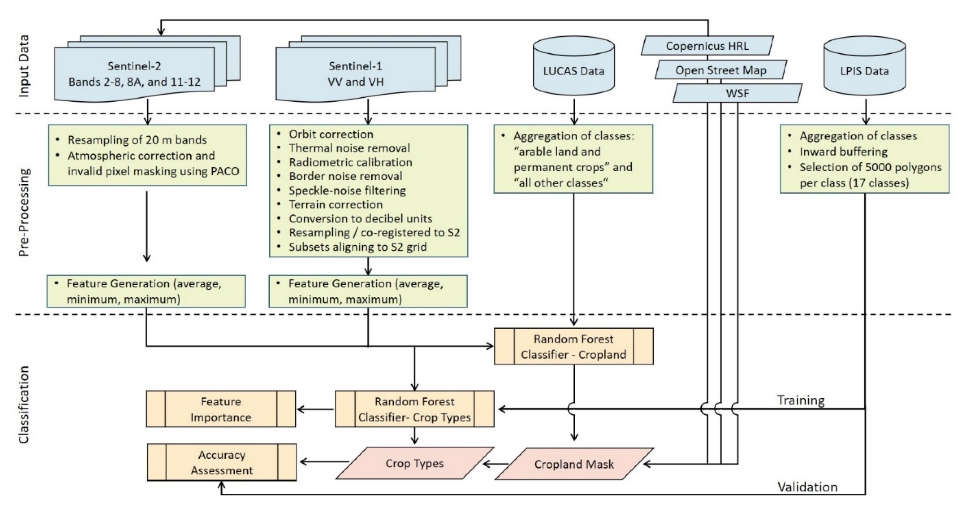
2.2. Satellite Data and Pre-Processing
2.3. Reference Data
2.4. Ancillary Data
2.5. Crop Type Classes
2.6. Crop Type Sampling Methodology
2.7. Crop Type Classification Approach
2.8. Accuracy Assessment
3. Results
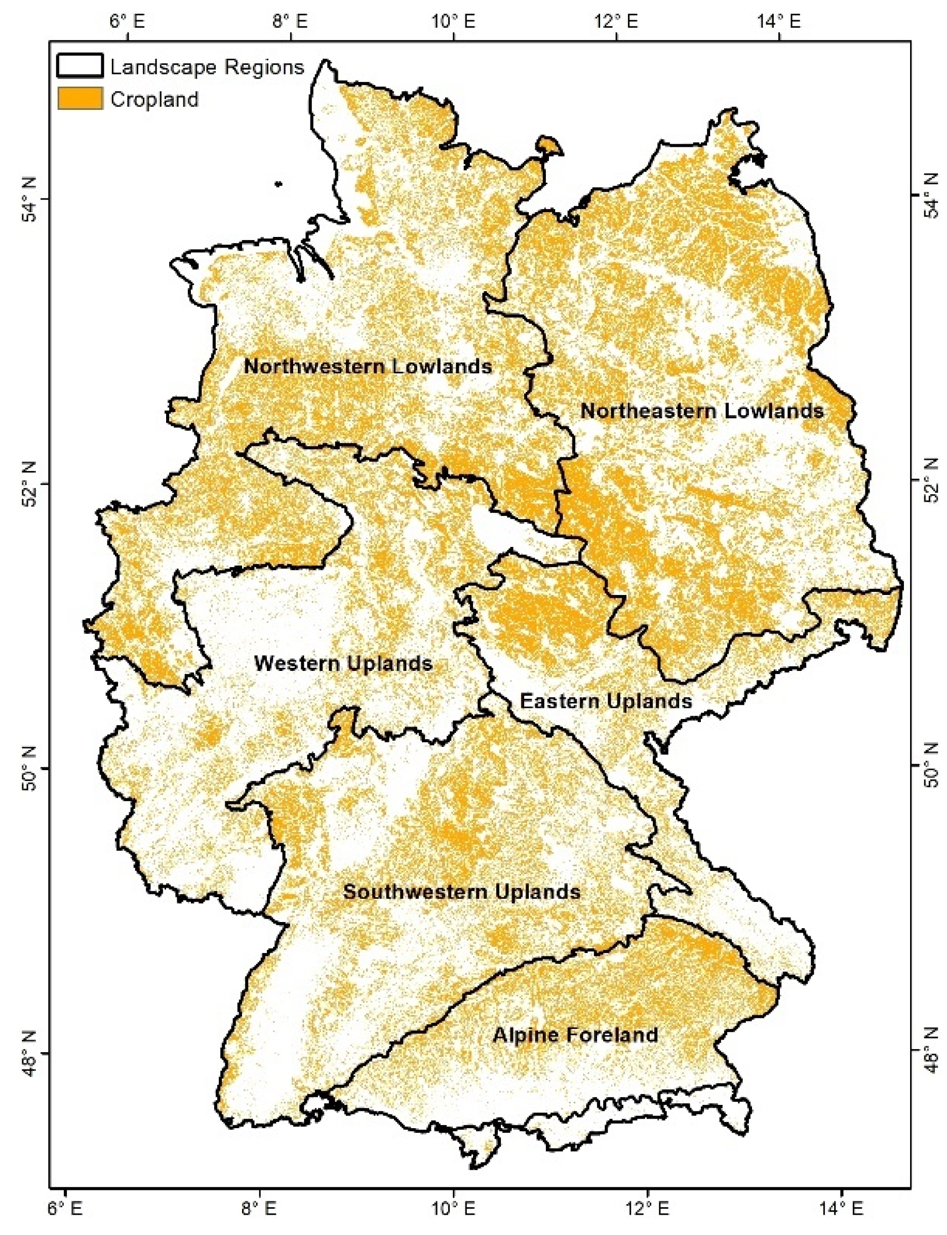
3.1. Cropland Mask
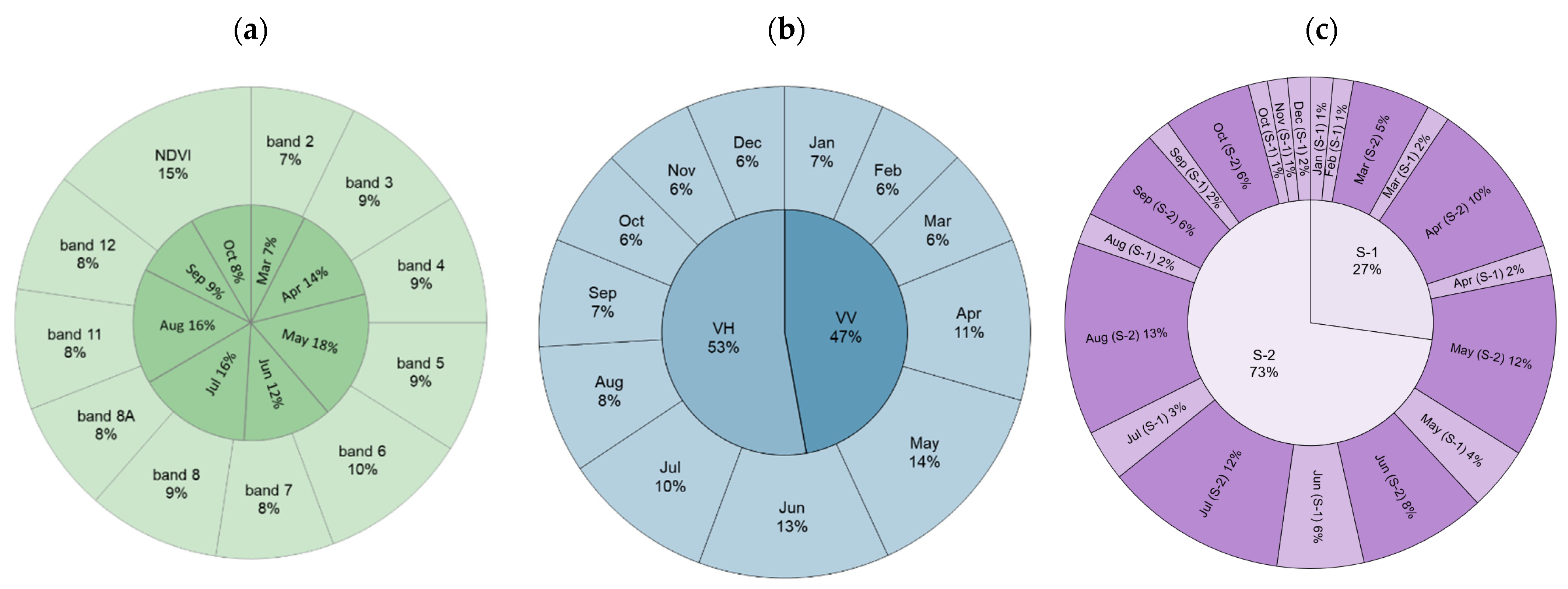
3.2. Overall Accuracy for Different Input Feature Sets and Overall Feature Importance
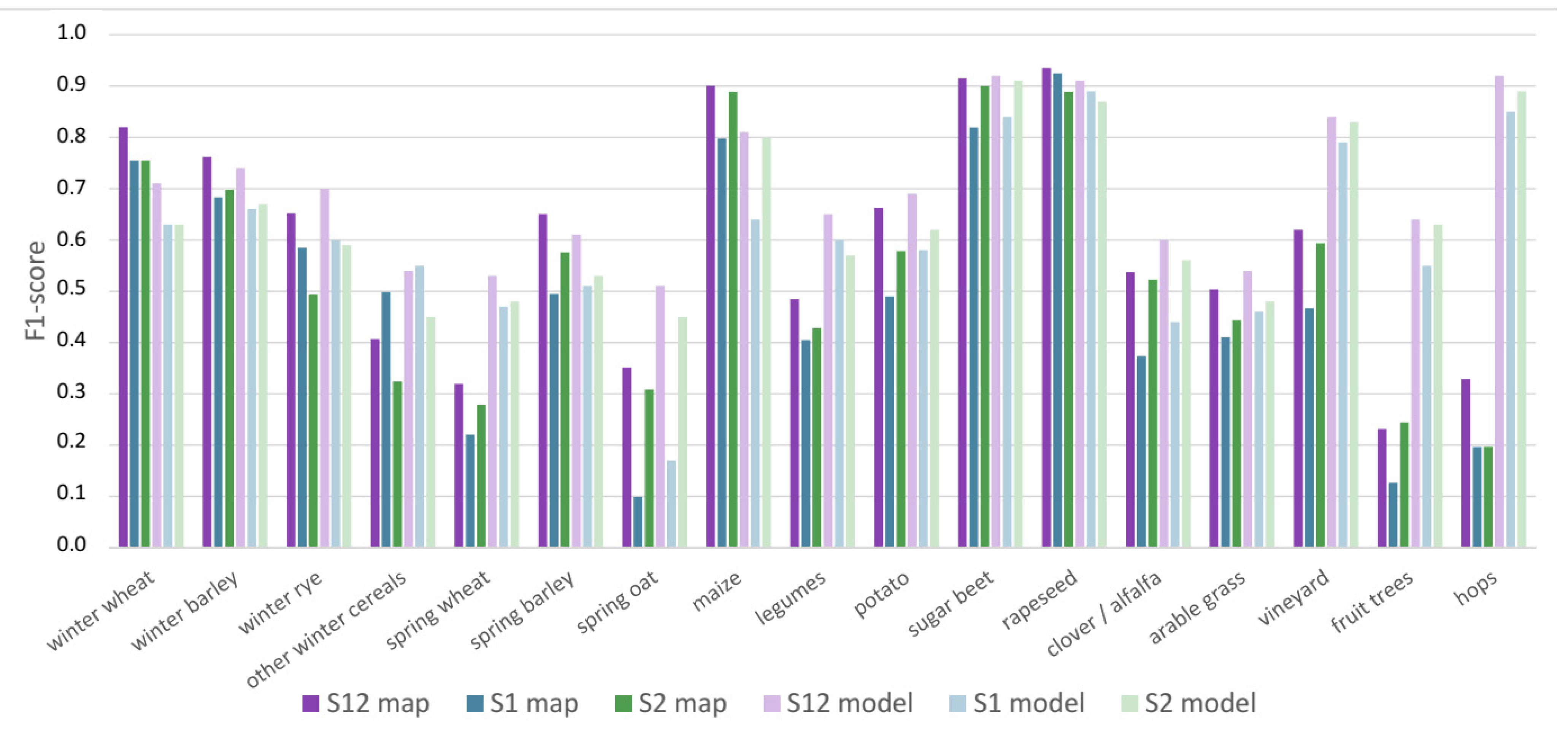
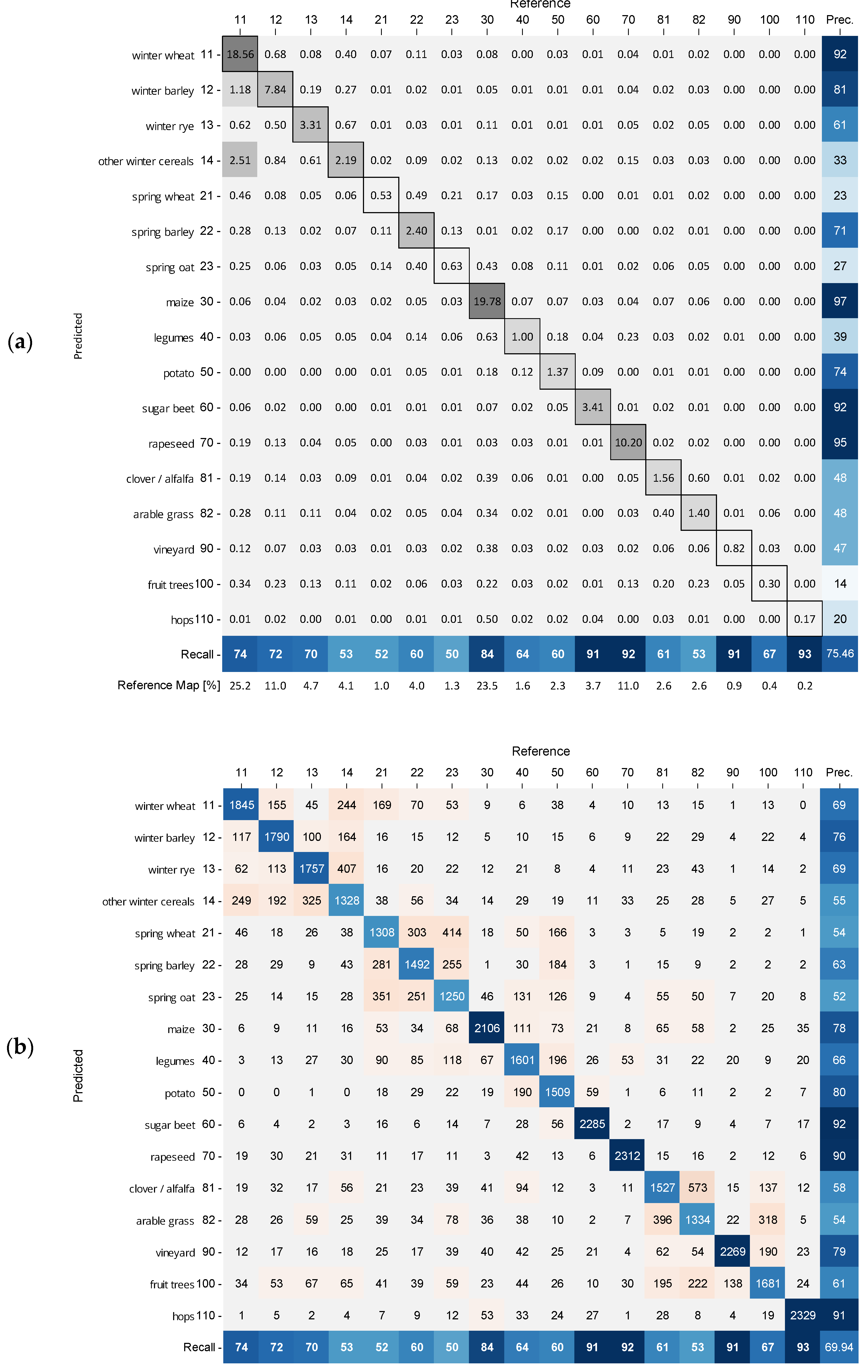
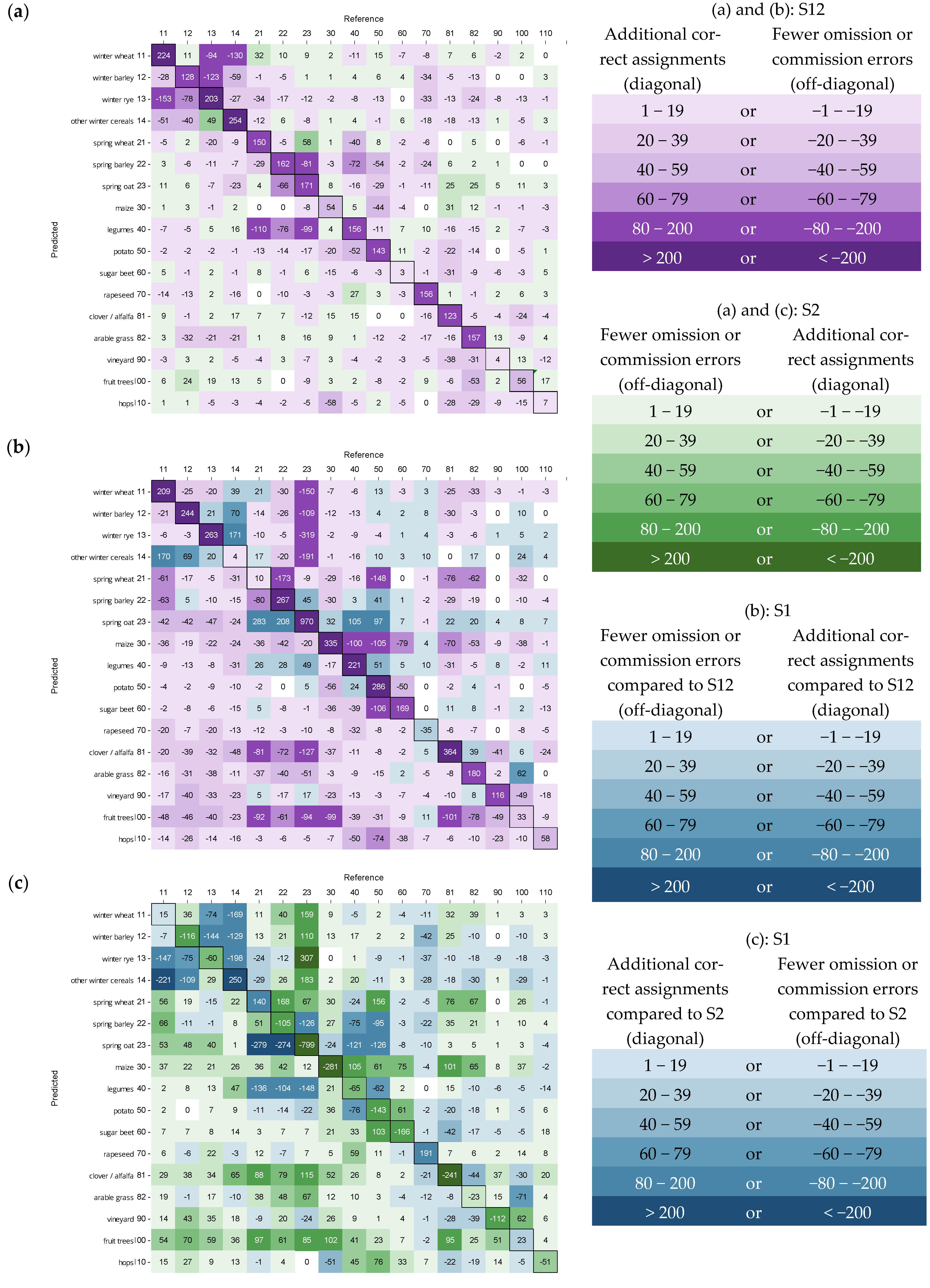
3.3. Class-Wise Accuracies and Influence of Sentinel-1 and Sentinel-2 Features on Class Separability
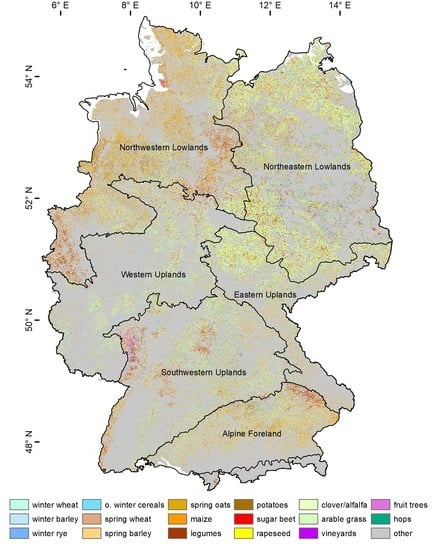
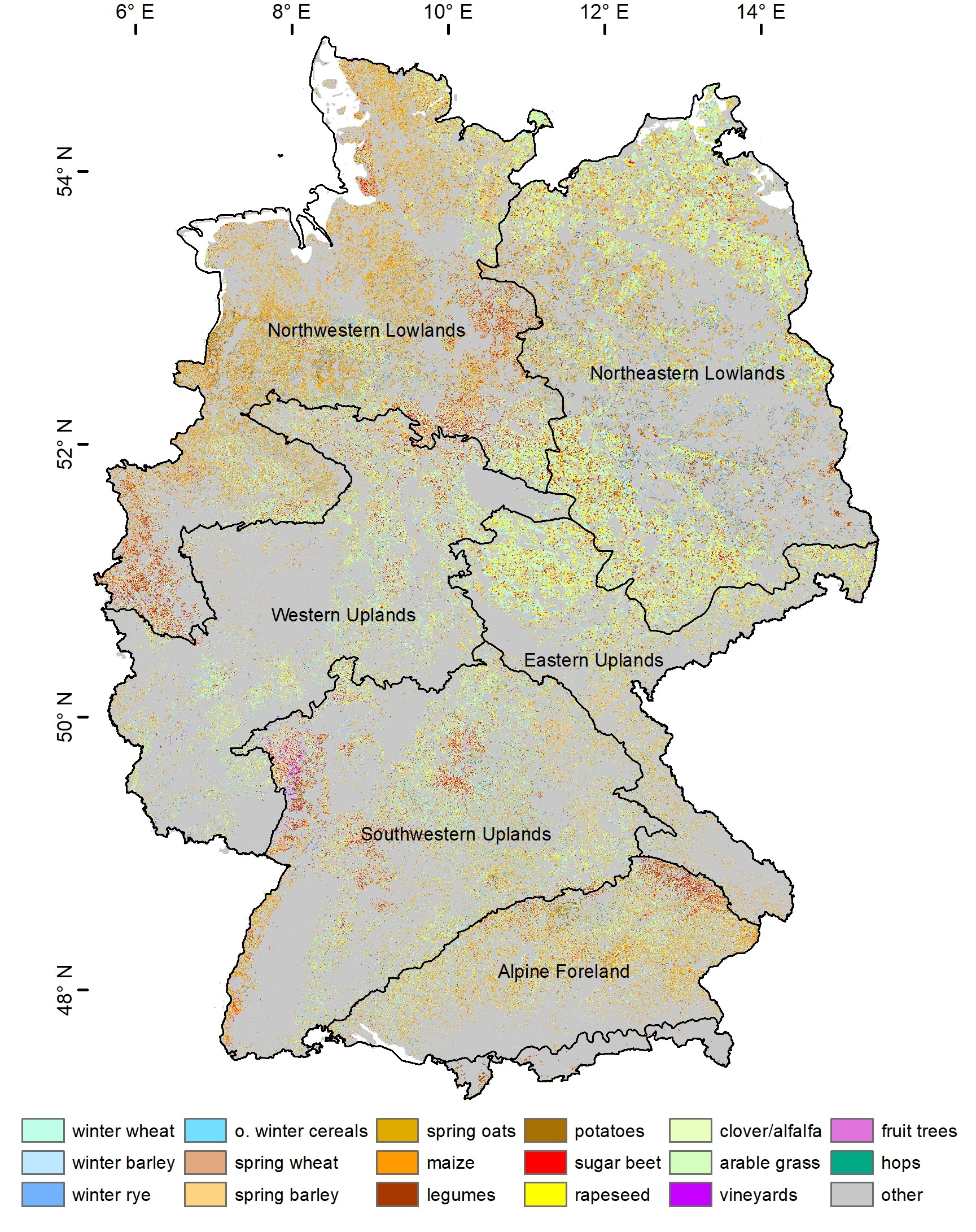
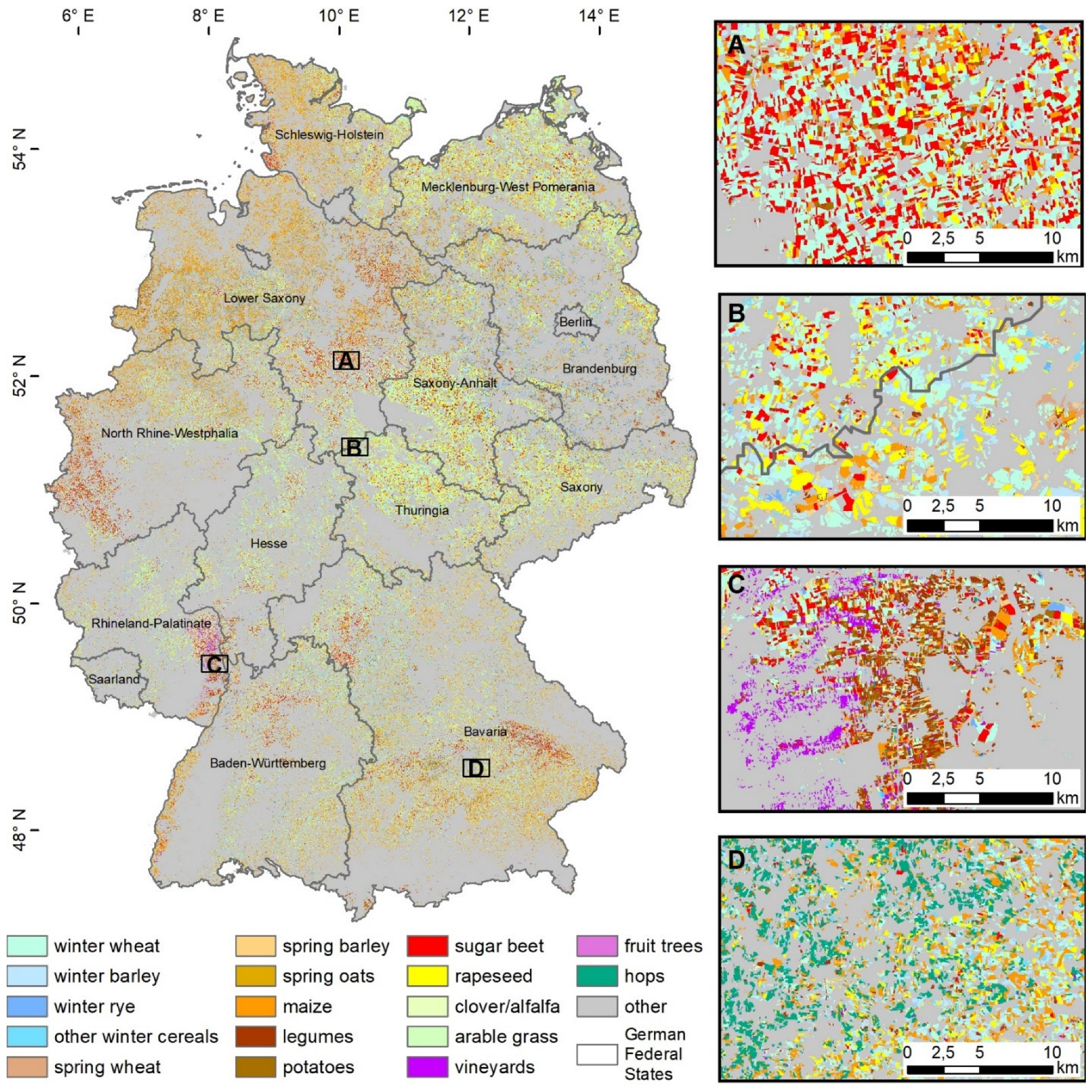
3.4. Country-Wide Crop Type Classification
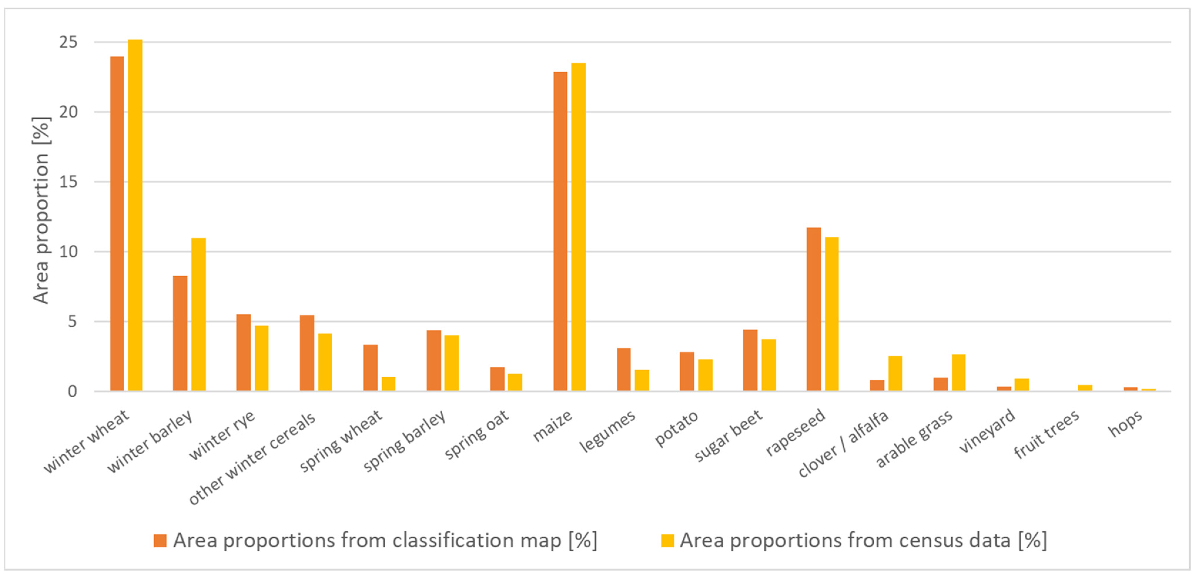
3.5. Comparison with National Agricultural Statistical Data
3.6. Crop Type Classifications for the Individual Landscape Regions
4. Discussion
4.1. Overall and Class-Specific Classification Accuracies
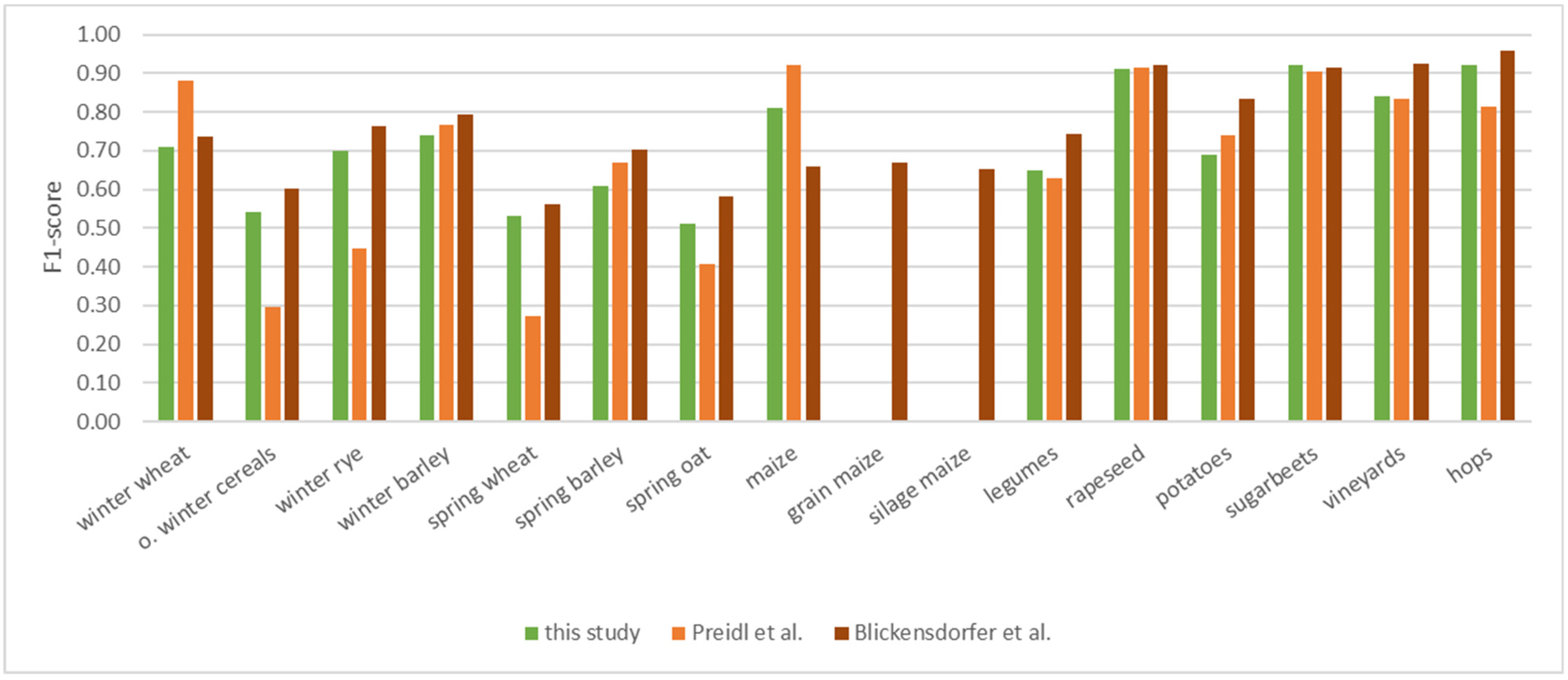
4.2. Comparison of Classification Accuracies and Method Complexity to Reference Studies
4.3. Combination of Optical and Radar Features
4.4. Regional Stratification
5. Conclusions
Supplementary Materials
Author Contributions
Funding
Data Availability Statement
Acknowledgments
Conflicts of Interest
References
- Statistisches Bundesamt (Destatis). Genesis-Online. Available online: https://www-genesis.destatis.de/genesis/online (accessed on 21 March 2022).
- Ray, D.K.; West, P.C.; Clark, M.; Gerber, J.S.; Prishchepov, A.V.; Chatterjee, S. Climate change has likely already affected global food production. PLoS ONE 2019, 14, e0217148. [Google Scholar] [CrossRef] [PubMed]
- Le Gouis, J.; Oury, F.-X.; Charmet, G. How changes in climate and agricultural practices influenced wheat production in Western Europe. J. Cereal Sci. 2020, 93, 102960. [Google Scholar] [CrossRef]
- Eckstein, D.; Künzel, V.; Schäfer, L.; Winges, M. Global Climate Risk Index 2020; Germanwatch, e.V.: Bonn, Germany, 2019; p. 44. [Google Scholar]
- Vitasse, Y.; Rebetez, M. Unprecedented risk of spring frost damage in Switzerland and Germany in 2017. Clim. Chang. 2018, 149, 233–246. [Google Scholar] [CrossRef]
- Lippert, C.; Krimly, T.; Aurbacher, J. A Ricardian analysis of the impact of climate change on agriculture in Germany. Clim. Chang. 2009, 97, 593. [Google Scholar] [CrossRef] [Green Version]
- Defourny, P.; Bontemps, S.; Bellemans, N.; Cara, C.; Dedieu, G.; Guzzonato, E.; Hagolle, O.; Inglada, J.; Nicola, L.; Rabaute, T.; et al. Near real-time agriculture monitoring at national scale at parcel resolution: Performance assessment of the Sen2-Agri automated system in various cropping systems around the world. Remote Sens. Environ. 2019, 221, 551–568. [Google Scholar] [CrossRef]
- Ibrahim, E.S.; Rufin, P.; Nill, L.; Kamali, B.; Nendel, C.; Hostert, P. Mapping Crop Types and Cropping Systems in Nigeria with Sentinel-2 Imagery. Remote Sens. 2021, 13, 3523. [Google Scholar] [CrossRef]
- Vuolo, F.; Neuwirth, M.; Immitzer, M.; Atzberger, C.; Ng, W.-T. How much does multi-temporal Sentinel-2 data improve crop type classification? Int. J. Appl. Earth Obs. Geoinf. 2018, 72, 122–130. [Google Scholar] [CrossRef]
- Immitzer, M.; Vuolo, F.; Atzberger, C. First Experience with Sentinel-2 Data for Crop and Tree Species Classifications in Central Europe. Remote Sens. 2016, 8, 166. [Google Scholar] [CrossRef]
- Hernandez, I.; Benevides, P.; Costa, H.; Caetano, M. Exploring Sentinel-2 for Land Cover and Crop Mapping in Portugal. Int. Arch. Photogramm. Remote Sens. Spat. Inf. Sci. 2020, 43, 83–89. [Google Scholar] [CrossRef]
- Belgiu, M.; Csillik, O. Sentinel-2 cropland mapping using pixel-based and object-based time-weighted dynamic time warping analysis. Remote Sens. Environ. 2018, 204, 509–523. [Google Scholar] [CrossRef]
- Mazzia, V.; Khaliq, A.; Chiaberge, M. Improvement in Land Cover and Crop Classification based on Temporal Features Learning from Sentinel-2 Data Using Recurrent-Convolutional Neural Network (R-CNN). Appl. Sci. 2019, 10, 238. [Google Scholar] [CrossRef] [Green Version]
- Paris, C.; Weikmann, G.; Bruzzone, L. Monitoring of Agricultural Areas by using Sentinel 2 Image Time Series and Deep Learning Techniques. In Proceedings of the SPIE 11533, Image and Signal Processing for Remote Sensing XXVI, Online, 21 September 2020. [Google Scholar]
- Račič, M.; Oštir, K.; Peressutti, D.; Zupanc, A.; Čehovin Zajc, L. Application of Temporal Convolutional Neural Network for the Classification of Crops on Sentinel-2 Time Series. Int. Arch. Photogramm. Remote Sens. Spat. Inf. Sci. 2020, 43, 1337–1342. [Google Scholar] [CrossRef]
- Rousi, M.; Sitokonstantinou, V.; Meditskos, G.; Papoutsis, I.; Gialampoukidis, I.; Koukos, A.; Karathanassi, V.; Drivas, T.; Vrochidis, S.; Kontoes, C.; et al. Semantically Enriched Crop Type Classification and Linked Earth Observation Data to Support the Common Agricultural Policy Monitoring. IEEE J. Sel. Top. Appl. Earth Obs. Remote Sens. 2021, 14, 529–552. [Google Scholar] [CrossRef]
- Sitokonstantinou, V.; Papoutsis, I.; Kontoes, C.; Arnal, A.; Andrés, A.P.; Zurbano, J.A. Scalable Parcel-Based Crop Identification Scheme Using Sentinel-2 Data Time-Series for the Monitoring of the Common Agricultural Policy. Remote Sens. 2018, 10, 911. [Google Scholar] [CrossRef] [Green Version]
- Turkoglu, M.O.; D’Aronco, S.; Perich, G.; Liebisch, F.; Streit, C.; Schindler, K.; Wegner, J.D. Crop mapping from image time series: Deep learning with multi-scale label hierarchies. Remote Sens. Environ. 2021, 264. [Google Scholar] [CrossRef]
- Belgiu, M.; Bijker, W.; Csillik, O.; Stein, A. Phenology-based sample generation for supervised crop type classification. Int. J. Appl. Earth Obs. Geoinf. 2021, 95, 102264. [Google Scholar] [CrossRef]
- Martini, M.; Mazzia, V.; Khaliq, A.; Chiaberge, M. Domain-Adversarial Training of Self-Attention-Based Networks for Land Cover Classification Using Multi-Temporal Sentinel-2 Satellite Imagery. Remote Sens. 2021, 13, 2564. [Google Scholar] [CrossRef]
- Gallo, I.; La Grassa, R.; Landro, N.; Boschetti, M. Sentinel 2 Time Series Analysis with 3D Feature Pyramid Network and Time Domain Class Activation Intervals for Crop Mapping. ISPRS Int. J. Geoinf. 2021, 10, 483. [Google Scholar] [CrossRef]
- Preidl, S.; Lange, M.; Doktor, D. Introducing APiC for regionalised land cover mapping on the national scale using Sentinel-2A imagery. Remote Sens. Environ. 2020, 240, 111673. [Google Scholar] [CrossRef]
- Rußwurm, M.; Körner, M. Self-attention for raw optical Satellite Time Series Classification. ISPRS J. Photogramm. Remote Sens. 2020, 169, 421–435. [Google Scholar] [CrossRef]
- Marszalek, M.; Lösch, M.; Körner, M.; Schmidhalter, U. Multi-temporal Crop Type and Field Boundary Classification with Google Earth Engine. Preprints 2020, 2020, 040316. [Google Scholar] [CrossRef]
- Piedelobo, L.; Hernández-López, D.; Ballesteros, R.; Chakhar, A.; Del Pozo, S.; González-Aguilera, D.; Moreno, M.A. Scalable pixel-based crop classification combining Sentinel-2 and Landsat-8 data time series: Case study of the Duero river basin. Agric. Syst. 2019, 171, 36–50. [Google Scholar] [CrossRef]
- Griffiths, P.; Nendel, C.; Hostert, P. Intra-annual reflectance composites from Sentinel-2 and Landsat for national-scale crop and land cover mapping. Remote Sens. Environ. 2019, 220, 135–151. [Google Scholar] [CrossRef]
- Heupel, K.; Spengler, D.; Itzerott, S. A Progressive Crop-Type Classification Using Multitemporal Remote Sensing Data and Phenological Information. PFG–J. Photogramm. Remote Sens. Geoinf. Sci. 2018, 86, 53–69. [Google Scholar] [CrossRef] [Green Version]
- Kyere, I.; Astor, T.; Graß, R.; Wachendorf, M. Agricultural crop discrimination in a heterogeneous low-mountain range region based on multi-temporal and multi-sensor satellite data. Comput. Electron. Agric. 2020, 179, 105864. [Google Scholar] [CrossRef]
- Orynbaikyzy, A.; Gessner, U.; Conrad, C. Crop type classification using a combination of optical and radar remote sensing data: A review. Int. J. Remote Sens. 2019, 40, 6553–6595. [Google Scholar] [CrossRef]
- Arias, M.; Campo-Bescós, M.Á.; Álvarez-Mozos, J. Crop Classification Based on Temporal Signatures of Sentinel-1 Observations over Navarre Province, Spain. Remote Sens. 2020, 12, 278. [Google Scholar] [CrossRef] [Green Version]
- d’Andrimont, R.; Verhegghen, A.; Lemoine, G.; Kempeneers, P.; Meroni, M.; van der Velde, M. From parcel to continental scale–A first European crop type map based on Sentinel-1 and LUCAS Copernicus in-situ observations. Remote Sens. Environ. 2021, 266, 112708. [Google Scholar] [CrossRef]
- Beriaux, E.; Jago, A.; Lucau-Danila, C.; Planchon, V.; Defourny, P. Sentinel-1 Time Series for Crop Identification in the Framework of the Future CAP Monitoring. Remote Sens. 2021, 13, 2785. [Google Scholar] [CrossRef]
- Mestre-Quereda, A.; Lopez-Sanchez, J.M.; Vicente-Guijalba, F.; Jacob, A.W.; Engdahl, M.E. Time-Series of Sentinel-1 Interferometric Coherence and Backscatter for Crop-Type Mapping. IEEE J. Sel. Top. Appl. Earth Obs. Remote Sens. 2020, 13, 4070–4084. [Google Scholar] [CrossRef]
- Nasirzadehdizaji, R.; Sanli, F.B.; Cakir, Z. Application of Sentinel-1 Multi-Temporal Data for Crop Monitoring and Mapping. Int. Arch. Photogramm. Remote Sens. Spat. Inf. Sci. 2019, 42, 803–807. [Google Scholar] [CrossRef] [Green Version]
- Planque, C.; Lucas, R.; Punalekar, S.; Chognard, S.; Hurford, C.; Owers, C.; Horton, C.; Guest, P.; King, S.; Williams, S.; et al. National Crop Mapping Using Sentinel-1 Time Series: A Knowledge-Based Descriptive Algorithm. Remote Sens. 2021, 13, 846. [Google Scholar] [CrossRef]
- Teimouri, N.; Dyrmann, M.; Jørgensen, R.N. A Novel Spatio-Temporal FCN-LSTM Network for Recognizing Various Crop Types Using Multi-Temporal Radar Images. Remote Sens. 2019, 11, 990. [Google Scholar] [CrossRef] [Green Version]
- Denize, J.; Hubert-Moy, L.; Pottier, E. Polarimetric SAR Time-Series for Identification of Winter Land Use. Sensors 2019, 19, 5574. [Google Scholar] [CrossRef] [Green Version]
- Gella, G.W.; Bijker, W.; Belgiu, M. Mapping crop types in complex farming areas using SAR imagery with dynamic time warping. ISPRS J. Photogramm. Remote Sens. 2021, 175, 171–183. [Google Scholar] [CrossRef]
- Valcarce-Diñeiro, R.; Arias-Pérez, B.; Lopez-Sanchez, J.M.; Sánchez, N. Multi-Temporal Dual- and Quad-Polarimetric Synthetic Aperture Radar Data for Crop-Type Mapping. Remote Sens. 2019, 11, 1518. [Google Scholar] [CrossRef] [Green Version]
- Woźniak, E.; Rybicki, M.; Kofman, W.; Aleksandrowicz, S.; Wojtkowski, C.; Lewiński, S.; Bojanowski, J.; Musiał, J.; Milewski, T.; Slesiński, P.; et al. Multi-temporal phenological indices derived from time series Sentinel-1 images to country-wide crop classification. Int. J. Appl. Earth Obs. Geoinf. 2022, 107, 102683. [Google Scholar] [CrossRef]
- Reuß, F.; Greimeister-Pfeil, I.; Vreugdenhil, M.; Wagner, W. Comparison of Long Short-Term Memory Networks and Random Forest for Sentinel-1 Time Series Based Large Scale Crop Classification. Remote Sens. 2021, 13, 5000. [Google Scholar] [CrossRef]
- Bargiel, D. A new method for crop classification combining time series of radar images and crop phenology information. Remote Sens. Environ. 2017, 198, 369–383. [Google Scholar] [CrossRef]
- Hütt, C.; Waldhoff, G.; Bareth, G. Fusion of Sentinel-1 with Official Topographic and Cadastral Geodata for Crop-Type Enriched LULC Mapping Using FOSS and Open Data. ISPRS Int. J. Geoinf 2020, 9, 120. [Google Scholar] [CrossRef] [Green Version]
- Kenduiywo, B.K.; Bargiel, D.; Soergel, U. Crop-type mapping from a sequence of Sentinel 1 images. Int. J. Remote Sens. 2018, 39, 6383–6404. [Google Scholar] [CrossRef]
- Sun, L.; Chen, J.; Guo, S.; Deng, X.; Han, Y. Integration of Time Series Sentinel-1 and Sentinel-2 Imagery for Crop Type Mapping over Oasis Agricultural Areas. Remote Sens. 2020, 12, 158. [Google Scholar] [CrossRef] [Green Version]
- Kpienbaareh, D.; Sun, X.; Wang, J.; Luginaah, I.; Bezner Kerr, R.; Lupafya, E.; Dakishoni, L. Crop Type and Land Cover Mapping in Northern Malawi Using the Integration of Sentinel-1, Sentinel-2, and PlanetScope Satellite Data. Remote Sens. 2021, 13, 700. [Google Scholar] [CrossRef]
- Moumni, A.; Lahrouni, A. Machine Learning-Based Classification for Crop-Type Mapping Using the Fusion of High-Resolution Satellite Imagery in a Semiarid Area. Scientifica 2021, 2021, 8810279. [Google Scholar] [CrossRef] [PubMed]
- Chakhar, A.; Hernández-López, D.; Ballesteros, R.; Moreno, M.A. Improving the Accuracy of Multiple Algorithms for Crop Classification by Integrating Sentinel-1 Observations with Sentinel-2 Data. Remote Sens. 2021, 13, 243. [Google Scholar] [CrossRef]
- Inglada, J.; Vincent, A.; Arias, M.; Marais-Sicre, C. Improved Early Crop Type Identification By Joint Use of High Temporal Resolution SAR And Optical Image Time Series. Remote Sens. 2016, 8, 362. [Google Scholar] [CrossRef] [Green Version]
- Kussul, N.; Lemoine, G.; Gallego, F.J.; Skakun, S.V.; Lavreniuk, M.; Shelestov, A.Y. Parcel-Based Crop Classification in Ukraine Using Landsat-8 Data and Sentinel-1A Data. IEEE J. Sel. Top. Appl. Earth Obs. Remote Sens. 2016, 9, 2500–2508. [Google Scholar] [CrossRef]
- Van Tricht, K.; Gobin, A.; Gilliams, S.; Piccard, I. Synergistic Use of Radar Sentinel-1 and Optical Sentinel-2 Imagery for Crop Mapping: A Case Study for Belgium. Remote Sens. 2018, 10, 1642. [Google Scholar] [CrossRef] [Green Version]
- Kussul, N.; Lavreniuk, M.; Skakun, S.; Shelestov, A. Deep Learning Classification of Land Cover and Crop Types Using Remote Sensing Data. IEEE Geosci. Remote. Sens. Lett. 2017, 14, 778–782. [Google Scholar] [CrossRef]
- Kussul, N.; Mykola, L.; Shelestov, A.; Skakun, S. Crop inventory at regional scale in Ukraine: Developing in season and end of season crop maps with multi-temporal optical and SAR satellite imagery. Eur. J. Remote. Sens. 2018, 51, 627–636. [Google Scholar] [CrossRef] [Green Version]
- Giordano, S.; Bailly, S.; Landrieu, L.; Chehata, N. Improved Crop Classification with Rotation Knowledge using Sentinel-1 and -2 Time Series. Photogramm. Eng. Remote Sens. 2020, 86, 431–441. [Google Scholar] [CrossRef]
- Ofori-Ampofo, S.; Pelletier, C.; Lang, S. Crop Type Mapping from Optical and Radar Time Series Using Attention-Based Deep Learning. Remote Sens. 2021, 13, 4668. [Google Scholar] [CrossRef]
- Blickensdörfer, L.; Schwieder, M.; Pflugmacher, D.; Nendel, C.; Erasmi, S.; Hostert, P. Mapping of crop types and crop sequences with combined time series of Sentinel-1, Sentinel-2 and Landsat 8 data for Germany. Remote Sens. Environ. 2022, 269, 112831. [Google Scholar] [CrossRef]
- Orynbaikyzy, A.; Gessner, U.; Mack, B.; Conrad, C. Crop Type Classification Using Fusion of Sentinel-1 and Sentinel-2 Data: Assessing the Impact of Feature Selection, Optical Data Availability, and Parcel Sizes on the Accuracies. Remote Sens. 2020, 12, 2779. [Google Scholar] [CrossRef]
- Orynbaikyzy, A.; Gessner, U.; Conrad, C. Spatial Transferability of Random Forest Models for Crop Type Classification Using Sentinel-1 and Sentinel-2. Remote Sens. 2022, 14, 1493. [Google Scholar] [CrossRef]
- Salehi, B.; Daneshfar, B.; Davidson, A.M. Accurate crop-type classification using multi-temporal optical and multi-polarization SAR data in an object-based image analysis framework. Int. J. Remote Sens. 2017, 38, 4130–4155. [Google Scholar] [CrossRef]
- Inglada, J.; Vincent, A.; Arias, M.; Tardy, B.; Morin, D.; Rodes, I. Operational High Resolution Land Cover Map Production at the Country Scale Using Satellite Image Time Series. Remote Sens. 2017, 9, 95. [Google Scholar] [CrossRef] [Green Version]
- Foerster, S.; Kaden, K.; Foerster, M.; Itzerott, S. Crop type mapping using spectral–temporal profiles and phenological information. Comput. Electron. Agric. 2012, 89, 30–40. [Google Scholar] [CrossRef] [Green Version]
- Kerner, H.; Sahajpal, R.; Skakun, S.; Becker-Reshef, I.; Barker, B.; Hosseini, M.; Puricelli, E.; Gray, P. Resilient in-season crop type classification in multispectral satellite observations using growth stage normalization. arXiv 2020. [Google Scholar] [CrossRef]
- Skakun, S.; Vermote, E.; Franch, B.; Roger, J.-C.; Kussul, N.; Ju, J.; Masek, J. Winter Wheat Yield Assessment from Landsat 8 and Sentinel-2 Data: Incorporating Surface Reflectance, Through Phenological Fitting, into Regression Yield Models. Remote Sens. 2019, 11, 1768. [Google Scholar] [CrossRef] [Green Version]
- DESTATIS. Landwirtschaftliche Betriebe, Ausgewählte Merkmale im Zeitvergleich. Available online: https://www.destatis.de/DE/Themen/Branchen-Unternehmen/Landwirtschaft-Forstwirtschaft-Fischerei/Landwirtschaftliche-Betriebe/Tabellen/ausgewaehlte-merkmale-zv.html (accessed on 21 April 2022).
- BMEL. Daten und Fakten-Land-, Forst- und Ernährungswirtschaft mit Fischerei und Wein- und Gartenbau. Available online: https://www.bmel.de/SharedDocs/Downloads/DE/Broschueren/Daten-und-Fakten-Landwirtschaft.pdf (accessed on 21 April 2022).
- German Environment Agency. Environment and Agriculture 2018. 2018. Available online: https://www.umweltbundesamt.de/sites/default/files/medien/421/publikationen/180608_uba_fl_umwelt_und_landwirtschaft_engl_bf_neu.pdf (accessed on 21 April 2022).
- ESA. Sentinel-2 User Handbook; ESA: Paris, France, 2015; p. 64. Available online: https://sentinel.esa.int/documents/247904/685211/Sentinel-2_User_Handbook (accessed on 21 April 2022).
- de Los Reyes, R.; Langheinrich, M.; Schwind, P.; Richter, R.; Pflug, B.; Bachmann, M.; Muller, R.; Carmona, E.; Zekoll, V.; Reinartz, P. PACO: Python-Based Atmospheric COrrection. Sensors 2020, 20, 1428. [Google Scholar] [CrossRef] [PubMed] [Green Version]
- Veci, L.; Prats-Iraola, P.; Scheiber, R.; Collard, F.; Fomferra, N.; Engdahl, M. The sentinel-1 toolbox. In Proceedings of the IEEE International Geoscience and Remote Sensing Symposium (IGARSS), Québec, QC, Canada, 14–18 July 2012; pp. 1–3. [Google Scholar]
- Dobrinić, D.; Gašparović, M.; Medak, D. Sentinel-1 and 2 Time-Series for Vegetation Mapping Using Random Forest Classification: A Case Study of Northern Croatia. Remote Sens. 2021, 13, 2321. [Google Scholar] [CrossRef]
- Ye, Y.; Yang, C.; Zhu, B.; Zhou, L.; He, Y.; Jia, H. Improving Co-Registration for Sentinel-1 SAR and Sentinel-2 Optical Images. Remote Sens. 2021, 13, 928. [Google Scholar] [CrossRef]
- Yan, X.; Zhang, Y.; Zhang, D.; Hou, N. Multimodal image registration using histogram of oriented gradient distance and data-driven grey wolf optimizer. Neurocomputing 2020, 392, 108–120. [Google Scholar] [CrossRef]
- EUROSTAT. Land Use and Coverage Area frame Survey-LUCAS. 2018. Available online: https://ec.europa.eu/eurostat/de/web/lucas (accessed on 21 April 2022).
- European Union. Copernicus Land Monitoring Service 2018. 2018. Available online: https://land.copernicus.eu/ (accessed on 21 April 2022).
- mundialis GmbH & Co. KG. Landcover Classification Map of Germany 2019 Based on Sentinel-2 Data. 2020. Available online: https://www.mundialis.de/en/deutschland-2019-landbedeckung-auf-basis-von-sentinel-2-daten/ (accessed on 21 April 2022).
- OpenStreetMap-Contributors. OpenStreetMap. 2021. Available online: https://planet.osm.org. (accessed on 21 April 2022).
- Marconcini, M.; Metz-Marconcini, A.; Üreyen, S.; Palacios-Lopez, D.; Hanke, W.; Bachofer, F.; Zeidler, J.; Esch, T.; Gorelick, N.; Kakarla, A.; et al. Outlining where humans live, the World Settlement Footprint 2015. Sci. Data 2020, 7, 242. [Google Scholar] [CrossRef]
- Meynen, E.; Schmithüsen, J.; Gellert, J.; Neef, E.; Müller-Miny, H.; Schultze, H.J. Handbuch der Naturräumlichen Gliederung Deutschlands; Bundesanstalt für Landeskunde und Raumforwschung: Bad Godesberg, Germany, 1953–1962. [Google Scholar]
- DESTATIS. Land- und Forstwirtschaft, Fischerei; Wachstum und Ernte-Feldfrüchte 2018. Available online: https://www.statistischebibliothek.de/mir/receive/DEHeft_mods_00096325 (accessed on 21 April 2022).
- DESTATIS. Land- und Forstwirtschaft, Fischerei; Wachstum und Ernte-Baumobst 2018. Available online: https://www.statistischebibliothek.de/mir/receive/DEHeft_mods_00095516 (accessed on 21 April 2022).
- DESTATIS. Land- und Forstwirtschaft, Fischerei; Wachstum und Ernte-Weinmost 2018. Available online: https://www.statistischebibliothek.de/mir/receive/DEHeft_mods_00104653 (accessed on 21 April 2022).
- Bayerische Landesanstalt für Landwirtschaft. Hopfen des Jahresheftes Agrarmärkte 2020. Available online: https://www.stmelf.bayern.de/mam/cms07/iem/dateien/16_hopfen__by__2020.pdf (accessed on 21 April 2022).
- Olofsson, P.; Foody, G.M.; Herold, M.; Stehman, S.V.; Woodcock, C.E.; Wulder, M.A. Good practices for estimating area and assessing accuracy of land change. Remote Sens. Environ. 2014, 148, 42–57. [Google Scholar] [CrossRef]
- Steinhausen, M.J.; Wagner, P.D.; Narasimhan, B.; Waske, B. Combining Sentinel-1 and Sentinel-2 data for improved land use and land cover mapping of monsoon regions. Int. J. Appl. Earth Obs. Geoinf. 2018, 73, 595–604. [Google Scholar] [CrossRef]
- Breiman, L. Random forests. Mach. Learn. 2001, 45, 5–32. [Google Scholar] [CrossRef] [Green Version]
- Pedregosa, F.; Varoquaux, G.; Gramfort, A.; Michel, V.; Thirion, B.; Grisel, O.; Blondel, M.; Prettenhofer, P.; Weiss, R.; Dubourg, V.; et al. Scikit-learn: Machine Learning in Python. J. Mach. Learn. Res. 2011, 12, 2825–2830. [Google Scholar]
- Hüttich, C.; Gessner, U.; Herold, M.; Strohbach, B.; Schmidt, M.; Keil, M.; Dech, S. On the Suitability of MODIS Time Series Metrics to Map Vegetation Types in Dry Savanna Ecosystems: A Case Study in the Kalahari of NE Namibia. Remote Sens. 2009, 1, 620–643. [Google Scholar] [CrossRef] [Green Version]
- Löw, F.; Michel, U.; Dech, S.; Conrad, C. Impact of feature selection on the accuracy and spatial uncertainty of per-field crop classification using Support Vector Machines. ISPRS J. Photogramm. Remote Sens. 2013, 85, 102–119. [Google Scholar] [CrossRef]
- Congalton, R.G. A review of assessing the accuracy of classifications of remotely sensed data. Remote Sens. Environ. 1991, 37, 35–46. [Google Scholar] [CrossRef]
- Sokolova, M.; Lapalme, G. A systematic analysis of performance measures for classification tasks. Inf. Processing Manag. 2009, 45, 427–437. [Google Scholar] [CrossRef]
- Stehman, S.V. Estimating area and map accuracy for stratified random sampling when the strata are different from the map classes. Int. J. Remote Sens. 2014, 35, 4923–4939. [Google Scholar] [CrossRef]
- Kontgis, C.; Schneider, A.; Ozdogan, M. Mapping rice paddy extent and intensification in the Vietnamese Mekong River Delta with dense time stacks of Landsat data. Remote Sens. Environ. 2015, 169, 255–269. [Google Scholar] [CrossRef]


| Crop Type | Class Code | LPIS Classes Included |
|---|---|---|
| winter wheat | 11 | winter wheat, durum wheat |
| winter barley | 12 | winter barley |
| winter rye | 13 | winter rye |
| other winter cereals | 14 | winter triticale, winter spelt |
| spring wheat | 21 | spring wheat |
| spring barley | 22 | spring barley |
| spring oat | 23 | spring oat |
| maize | 30 | maize, maize (biogas), maize (silage), grain maize, maize with flower strip/hunting aisle |
| legumes | 40 | peas, beans, peas-beans mixtures, soy, lupins |
| potato | 50 | potatoes, starch potato, seed potato |
| sugar beet | 60 | sugar beet |
| rapeseed | 70 | winter rapeseed |
| clover/alfalfa | 81 | clover sorts, alfalfa, clover/alfalfa-grass-mixtures |
| arable grass | 82 | arable grass |
| vineyard | 90 | vineyard |
| fruit trees | 100 | stone fruits, pomaceous fruits, orchard meadows |
| hops | 110 | hops |
| S12 | S1 | S2 | |
|---|---|---|---|
| Map accuracy [%] | 75.5 | 66.6 | 69.7 |
| Model accuracy [%] | 69.9 | 61.2 | 64.9 |
| Crop | Class | NWL | NEL | WUL | EUL | SWUL | AFL | Average Regions | GER |
|---|---|---|---|---|---|---|---|---|---|
| winter wheat | 11 | 0.76 | 0.80 | 0.78 | 0.73 | 0.75 | 0.83 | 0.78 | 0.82 |
| winter barley | 12 | 0.75 | 0.75 | 0.77 | 0.70 | 0.71 | 0.86 | 0.76 | 0.76 |
| winter rye | 13 | 0.57 | 0.60 | 0.26 | - | 0.43 | - | 0.47 | 0.65 |
| o. winter cereals | 14 | 0.42 | 0.19 | 0.35 | 0.28 | 0.42 | 0.40 | 0.34 | 0.41 |
| spring wheat | 21 | 0.26 | 0.35 | 0.30 | 0.30 | 0.12 | - | 0.27 | 0.32 |
| spring barley | 22 | 0.54 | - | 0.65 | 0.72 | 0.72 | 0.71 | 0.67 | 0.65 |
| spring oat | 23 | 0.12 | 0.27 | 0.38 | 0.40 | 0.41 | 0.47 | 0.34 | 0.35 |
| maize | 30 | 0.93 | 0.80 | 0.89 | 0.91 | 0.87 | 0.91 | 0.89 | 0.90 |
| legumes | 40 | 0.54 | 0.49 | 0.51 | 0.70 | 0.53 | 0.56 | 0.56 | 0.48 |
| potato | 50 | 0.84 | 0.61 | - | - | 0.52 | 0.80 | 0.70 | 0.66 |
| sugar beet | 60 | 0.94 | 0.89 | 0.93 | - | 0.92 | 0.93 | 0.92 | 0.91 |
| rapeseed | 70 | 0.93 | 0.97 | 0.91 | 0.96 | 0.92 | 0.94 | 0.94 | 0.93 |
| clover/alfalfa | 81 | - | - | - | 0.69 | 0.69 | 0.62 | 0.67 | 0.54 |
| arable grass | 82 | 0.65 | 0.47 | - | - | - | - | 0.56 | 0.50 |
| vineyard | 90 | - | - | 0.75 | - | 0.81 | - | 0.78 | 0.62 |
| fruit trees | 100 | 0.30 | 0.15 | 0.21 | 0.16 | 0.37 | 0.72 | 0.32 | 0.23 |
| hops | 110 | - | - | - | - | - | 0.50 | 0.50 | 0.33 |
| Overall accuracy | 76.6 | 73.8 | 73.0 | 72.1 | 72.1 | 80.5 | 74.7 | 75.5 |
| PRE | BLI | This Study | |
|---|---|---|---|
| year(s) | 2016 | 2017–2019 | 2018 |
| spatial resolution [m] | 20 | 10 | 10 |
| reference data | LPIS data from 7 Federal States + local patches | LPIS data from 4–5 Federal States | LPIS data from 15 Federal States |
| sampling scheme | proportional | equal | equal |
| number of crop classes | 19 | 23 | 17 |
| permanent grassland included | yes | yes | no |
| number of input features | 54–126 (in 64–16,383 model runs) | 483 | 336 |
| input source types | optical | optical + radar + topography + climate + meteorology | optical + radar |
| regionalization | yes | no | no |
Publisher’s Note: MDPI stays neutral with regard to jurisdictional claims in published maps and institutional affiliations. |
© 2022 by the authors. Licensee MDPI, Basel, Switzerland. This article is an open access article distributed under the terms and conditions of the Creative Commons Attribution (CC BY) license (https://creativecommons.org/licenses/by/4.0/).
Share and Cite
Asam, S.; Gessner, U.; Almengor González, R.; Wenzl, M.; Kriese, J.; Kuenzer, C. Mapping Crop Types of Germany by Combining Temporal Statistical Metrics of Sentinel-1 and Sentinel-2 Time Series with LPIS Data. Remote Sens. 2022, 14, 2981. https://doi.org/10.3390/rs14132981
Asam S, Gessner U, Almengor González R, Wenzl M, Kriese J, Kuenzer C. Mapping Crop Types of Germany by Combining Temporal Statistical Metrics of Sentinel-1 and Sentinel-2 Time Series with LPIS Data. Remote Sensing. 2022; 14(13):2981. https://doi.org/10.3390/rs14132981
Chicago/Turabian StyleAsam, Sarah, Ursula Gessner, Roger Almengor González, Martina Wenzl, Jennifer Kriese, and Claudia Kuenzer. 2022. "Mapping Crop Types of Germany by Combining Temporal Statistical Metrics of Sentinel-1 and Sentinel-2 Time Series with LPIS Data" Remote Sensing 14, no. 13: 2981. https://doi.org/10.3390/rs14132981