Rayleigh Lidar Signal Denoising Method Combined with WT, EEMD and LOWESS to Improve Retrieval Accuracy

Abstract

Lidar is an active remote sensing technology that has many advantages, but the echo lidar signal is extremely susceptible to noise and complex atmospheric environment, which affects the effective detection range and retrieval accuracy. In this paper, a wavelet transform (WT) and locally weighted scatterplot smoothing (LOWESS) based on ensemble empirical mode decomposition (EEMD) for Rayleigh lidar signal denoising was proposed. The WT method was used to remove the noise in the signal with a signal-to-noise ratio (SNR) higher than 16 dB. The EEMD method was applied to decompose the remaining signal into a series of intrinsic modal functions (IMFs), and then detrended fluctuation analysis (DFA) was conducted to determine the threshold for distinguishing whether noise or signal was the main component of the IMFs. Moreover, the LOWESS method was adopted to remove the noise in the IMFs component containing the signal, and thus, finely extract the signal. The simulation results showed that the denoising effect of the proposed WT-EEMD-LOWESS method was superior to EEMD-WT, EEMD-SVD and VMD-WOA. Finally, the use of WT-EEMD-LOWESS on the measured lidar signal led to significant improvement in retrieval accuracy. The maximum error of density and temperature retrievals was decreased from 1.36% and 125.79 K to 1.1% and 13.84 K, respectively.

1. Introduction

As an active remote sensing technology, lidar is widely used in autonomous driving, target detection and atmospheric detection, which has the characteristics of high spatial resolution and detection sensitivity [1,2,3,4]. In recent years, the middle atmosphere has received increasing attention. Rayleigh lidar, employing Rayleigh backscattering from atmospheric molecules, has become an effective means for studying middle atmosphere [5,6,7]. However, both the exponential decrease in number density with altitude and the spherical scattered light result in a decrease in lidar echo signal with the altitude squared, severely limiting the effective detection range and retrieval accuracy [8]. Moreover, strong background sunlight noise, dark current noise, and thermal noise interfere with the lidar echo signal [9]. Consequently, the signal-to-noise ratio at high altitudes is too low to retrieve correctly, so the lidar backscattering signal must be denoised.

In the last few decades, many researchers have paid attention to the processing of nonlinear and non-stationary lidar echo signal. The moving averages technique, a low-pass filtering method, is the simplest and most direct denoising method. However, on the one hand, the ideal filter will inevitably depend on the particular scene. On the other hand, this method will create extra errors due to the smearing of resolvable atmospheric structure [10]. Han et al. used the Kalman filtering method to derive water vapor profiles using surface in situ and Raman measurements, but this method may cause retrieval errors in cases of rapidly changing environments [11]. The WT method can decompose the signal into different frequency terms through multiscale analysis, but the main limitations are the selection of suitable wavelet basis functions and the decomposition level according to a particular scene [12,13].

Empirical mode decomposition (EMD) is widely used in the processing of non-stationary signals, due to the fact that its decomposition entirely depends on the signal itself and does not need any priori information [14,15]. Through EMD, a complex signal can be decomposed into a series of IMFs and a residual. The research on EMD mostly focuses on distinguishing whether noise or signal is the main component of the IMFs, or overcoming the shortcomings of EMD, such as modal aliasing and end effects. To solve these problems, Tian et al. suggested typical range (TR) and low-frequency fraction (LFF) as the reference principles to decide how many high-frequency IMFs should be removed as noise [16], and Wu et al. proposed EEMD to effectively suppress modal aliasing [17].

Variational mode decomposition (VMD) is a new method for decomposing signals adaptively [18]. Compared with EMD, VMD is a non-recursive decomposition algorithm, which can overcome the modal aliasing problem and embody Wiener filtering characteristics. In the VMD technique, the selection of the decomposition mode number and quadratic penalty is performed through an optimization algorithm [19]. In addition, the application of machine learning and neural networks for signal denoising has received extensive attention due to their adaptability to include prior information [20]. Sreekanth et al. adopted the dictionary learning technique in denoising lidar signal [21].

In the past, most studies focused on the lidar echo signal with a low signal-to-noise ratio, while ignoring the overall relevance. However, in engineering, it is always necessary to process the lidar echo signal within a certain height range, and therefore the signal-to-noise ratio has a large dynamic range. Since the single denoising method has its own advantages and shortcomings as described above, it is necessary to combine several denoising algorithms for improving the denoising performance. Furthermore, it is more convincing to use the simulated lidar echo signal to verify the effectiveness of the proposed algorithm than to use the synthetic signal.

In this paper, a WT and LOWESS based on the EEMD algorithm, called WT-EEMD-LOWESS, was proposed to extend the effective detection range and improve retrieval accuracy. The proposed method utilized the WT method to remove the noise in the signal with a signal-to-noise ratio higher than 16 dB. The EEMD method was applied to decompose the remaining signal into a series of IMFs, and the signal was reconstructed by using the DFA. Moreover, the LOWESS method was adopted to finely extract the signal in the reconstructed signal. The lidar simulation system with a typical integration time of 1200 s validated the feasibility of the WT-EEMD-LOWESS model. Then, the simulation experiment verified that our algorithm can be effectively applied to the lidar echo signal with different integration times. Finally, the denoising algorithm was investigated on the real Rayleigh lidar signal and experimental results showed that the WT-EEMD-LOWESS method can be directly adapted to engineering.

2. Rayleigh Lidar Simulation System

To select different yet available denoising methods for echo signal with different signal-to-noise ratios, the noisy lidar echo signal was simulated for comparison experiments. In the case of the Rayleigh lidar system, the return signal can be described as follows:

$$N_R(\lambda ,R)=\left(\frac{E_0}{hc/\lambda }\right)\left[{\sigma }_{180}(\lambda ,R)n\left(R\right)\Delta R\right]\frac{A}{R^2}\left[\eta \left(\lambda \right)T_t{T}_r{T}^2(\lambda ,R)G\left(R\right)\right]+N_B$$

(1)

where $N_R(\lambda ,R)$ is the number of received photons, when the wavelength of emitted laser is $\lambda$ and the detection distance is R; $E_0$ is pulse energy of the emitted laser; h is Plank’s constant; ${\sigma }_{180}(\lambda ,R)$ is the backscatter cross-section, ${\sigma }_{180}(\lambda ,R)=\frac{1}{4\pi }\times \frac{3}{2}\times 5.16\times {10}^{-31}{\mathrm{m}}^{-2}$; $n\left(R\right)$ is the number density of atmospheric molecules; $\Delta R$ is range resolution; A is receiving area of telescope; $\eta \left(\lambda \right)$ is detector quantum efficiency; $T_t$ and $T_r$ represent transmitting and receiving optical efficiencies, respectively; $T^2(\lambda ,R)$ is two-way atmospheric transmittance; $G\left(R\right)$ is geometric overlap factor; $N_B$ is the noise. The first term of the expression represents the number of emitted photons, the second term indicates the probability of backscattering of atmospheric molecules, the third term represents the ability of the detector to accept backscattered light and the last term stands for the system efficiency and transmittance. The schematic of the Rayleigh lidar system is illustrated in Figure 1.

The lidar signal is inevitably affected by noise during the detection process. The main sources of noise are background radiation noise, detector thermal noise and shot noise. The calculation formulas of background radiation noise $N_b$ and detector thermal noise $N_d$ are as follows:

$$N_b=\frac{\eta \lambda }{hc}{P}_b{\left(\frac{{\theta }_R}{2}\right)}^2\Delta \lambda A\Delta t{T}_r$$

(2)

$$N_d=CPS·\Delta t$$

(3)

where $P_b$ is the radiances of the sky, which were calculated using the MODTRAN software [22]; ${\theta }_R$ is the field of view of the receiving telescope; $\Delta \lambda$ is the bandwidth of the filter; $CPS$ is the dark count of the detector; $\Delta t$ is the acquisition time of the system.

Table 1. Simulation parameters of lidar system.

System Parameter	Value
Laser pulse energy/mJ	40
Telescope diameter/mm	350
Field of view/$\mathsf{\mu }$rad	165
Detection quantum efficiency	0.5
Total optical transmittance	0.4
Dark counts/counts per second	50
Range resolution/m	100
Filter bandwidth/nm	0.25
Pulse repetition frequency/Hz	50
Platform height/km	20

lists the parameters of our simulation system.

Shot noise follows a Poisson distribution. Therefore, when using the lidar equation to simulate the echo signal, Poisson noise needs to be added. Since the Rayleigh signal per laser pulse is too weak, averaging the pulses or integrating them is often used to increase the signal-to-noise ratio. Figure 2 shows the ideal echo signal obtained from the simulation and the noisy signal after subtracting the background radiation noise under the condition that the platform height is 20 km, the measurement altitude range is 30–70 km, and the integration time is 1200 s.

3. Methodology Descriptions

3.1. Brief Description of the WT Algorithm

Wavelet transform is developed on the basis of short-time Fourier transform and has good time-frequency localization characteristics. Compared with Fourier transform, which only has sine or cosine function as a basis, the types of wavelet basis are diverse. Previous experiments have proved that “$dB4$” and “$Sym4$” have achieved good results in the field of lidar signal processing.

In the wavelet threshold denoising, the raw signal is divided into approximation and detail coefficients. The orthogonal wavelet basis can mainly concentrate useful signal energy in some large wavelet coefficients. Therefore, the employment of threshold can retain the large useful signal coefficients and zero or shrink the the small noise coefficients, so as to denoise. In practice, the selection of the wavelet basis, the decomposition level and threshold value is a key point in algorithm design. The specific steps of wavelet threshold denoising are as follows:

Step 1: According to the characteristics of Rayleigh scattering echo signal, the proper wavelet basis and decomposition layer number N are selected, and the original return lidar data is decomposed with N layers based on wavelet transformation.

Step 2: Selecting the soft threshold method to carry on the threshold quantization processing for the high frequency coefficients from layer 1 to layer N by different threshold value of each decomposition layer.

Step 3: The low-frequency coefficient of the Nth layer and all high-frequency coefficients of each layer after wavelet threshold processing are reconstructed by inverse wavelet transformation, and the required signal is obtained.

3.2. Basic Theory of EEMD

EEMD is an improved algorithm of EMD, so the EMD algorithm is introduced first. The EMD method can adaptively decompose signals into a series of IMFs and a residual component based on the local characteristic time scale of the signal itself, which is given by

$$x\left(t\right)=\sum _{i=1}^{n}im{f}_i+r_n$$

(4)

Each IMF stands for the information on different scales of the original signal and must satisfy two conditions: (1) the number of extrema and zero crossings must either be equal or differ by one at most; (2) at any point, the mean value of the envelope defined by the local maxima and minima is zero. The first condition is a common signal analysis requirement for narrowband signals and the second condition ensures the local symmetry of the IMFs.

For any original signals $x\left(t\right)$, the procedure of EMD can be described as follows:

1.

Identifying the local extrema of $x\left(t\right)$.

2.

Using the cubic spline interpolation function to form the upper envelope $U\left(t\right)$ and the lower envelope $L\left(t\right)$.

3.

Calculating the mean value $m\left(t\right)$ of the upper and lower envelopes.

$$m\left(t\right)=\left[U\right(t)+L(t\left)\right]/2$$

(5)

4.

Denoting the difference in value between $x\left(t\right)$ and $m\left(t\right)$ as $h\left(t\right)$. If $h\left(t\right)$ satisfies conditions for IMFs, then $h\left(t\right)$ is defined as the first IMF. If not, $x\left(t\right)$ is represented as $h\left(t\right)$. Repeating the steps 1 to 3 K times until $h_K\left(t\right)=h_{K-1}\left(t\right)-m_{K-1}\left(t\right)$ meets IMF conditions and $h_K\left(t\right)$ will be the first IMF of the signal.

$$h\left(t\right)=x\left(t\right)-m\left(t\right)$$

(6)

5.

Separating the first IMF from $x\left(t\right)$. The residue item $r\left(t\right)$ can be computed with the following equation:

$$r\left(t\right)=x\left(t\right)-\mathrm{im}{\mathrm{f}}_1\left(t\right)$$

(7)

If $r\left(t\right)$ does not become a monotone function or the number of extrema is less than one or equal to one, $x\left(t\right)$ is replaced by $r\left(t\right)$. Repeating steps 1 to 4 n times, the n IMFs of $x\left(t\right)$ will be computed.

In order to solve modal aliasing problems of EMD, the EEMD algorithm, an effective noise-aided data analysis (NADA) method, adds white noise to the original signal by using the zero-mean characteristic of white noise. Because the white noise spectrum is evenly distributed, the white-noise signals will be automatically distributed to the appropriate reference scales. The specific procedure of the EEMD method is expressed as follows:

1.

Adding white noise, which follows a normal distribution with mean 0 and standard deviation $\sigma$, N times to the original signal $x\left(t\right)$.Then, the new data series can be computed as follows:

$$x_i\left(t\right)=x\left(t\right)+\sum _{j=1}^N\sigma n_j\left(t\right),n_j\left(t\right)\sim N(0,1)$$

(8)

2.

Decomposing the signal added with Gaussian white noise by EMD to obtain the ith set of decomposition results, which includes IMF components $c_{ij}\left(t\right)$ (j = 1, 2, …, m) and a residual $r_i\left(t\right)$.

3.

Repeating the above steps n times, the overall average values $c_j\left(t\right)$ and $r\left(t\right)$ are used as the results of the jth IMF component and the residual decomposed by EEMD, respectively.

$$c_j\left(t\right)=\frac{1}{n}\sum _{i=1}^n{c}_{ij}\left(t\right)$$

(9)

$$r\left(t\right)=\frac{1}{n}\sum _{i=1}^n{r}_i\left(t\right)$$

(10)

3.3. Principle of DFA

Selecting specific IMF components for superposition can form high-pass, low-pass and band-pass filters. Because the signal is concentrated on the low-frequency IMFs while noise is devoted to the high-frequency IMFs, denoising can be achieved by discarding some high-frequency components. DFA is a scaling analysis method to study long-range dependency for the non-stationary signal. DFA is utilized as a reliable metric to determine noisy IMFs resulting from the EMD [23]. Therefore, in this paper, DFA is used to distinguish whether noise or signal is the main component of the IMFs.

For a given time series $\left\{v\left(i\right),i=1,2,\cdots ,N\right\}$ with the length N, the main procedure of the DFA method is expressed as follows:

1.

Integrating the time series of the mean detached signal and the cumulative series $y\left(n\right)$ can be computed as follows:

$$y\left(k\right)=\sum _{i=1}^N[v\left(i\right)-\overline{v}],k=1,2,\cdots ,N$$

(11)

where $\overline{v}$ is the average of $v\left(i\right)$, $\overline{v}=\frac{1}{N}{\displaystyle \sum _{i=1}^N}v\left(i\right)$.

2.

The integrated series $y\left(n\right)$ was then divided into equal and non-overlapping windows of length n. For each window, the local linear trend $y_n\left(k\right)$ is calculated by a polynomial fitting of order l. The root mean square fluctuation $F\left(n\right)$ is given by the equation

$$F\left(n\right)=\sqrt{\frac{1}{N}\sum _{k=1}^N{[y\left(k\right)-y_n\left(k\right)]}^2}$$

(12)

3.

The scaling exponent $\alpha$ is calculated as a slope of the curve $log\left(F\right(n\left)\right)/log\left(n\right)$ as follows:

$$F\left(n\right)\propto n^{\alpha }$$

(13)

The scaling exponent $\alpha$ is related to the Hurst exponent H, which reflects the correlation of time series. The value $\alpha =0.5$ indicates that the time series is uncorrelated (white noise). $0<\alpha <0.5$ indicates that the time series is noise, which has short-range correlation and poor self-similarity between local and global data sequences. $\alpha >0.5$ represents the time series signal, which has long-range correlation.

3.4. Brief Description of the LOWESS Method

When processing lidar echo signals, it is expected to be less sensitive to photon fluctuations mainly caused by shot noise without distorting the signal. The LOWESS algorithm, first proposed by Cleveland in 1979 [24], effectively solves this problem. With the LOWESS method, the value of each point is an iterative weighted least square regression through a nearby data point within a specified span. The steps of the LOWESS method are as follows:

1.

Estimating the span width, which usually contains more than 13 data points and the initial weight of points $(x_i,y_i)$ within the span width is defined as a cubic weighting function as follows:

$$w_i=\left\{\begin{array}{c}\left(1-{\left|\frac{x-x_i}{d\left(x\right)}\right|}^3,\left|\frac{x-x_i}{d\left(x\right)}\right|\le 1\right)\\ 0,\left|\frac{x-x_i}{d\left(x\right)}\right|>1\end{array}\right\}$$

(14)

where $d\left(x\right)$ is the furthest distance between x and $x_i$ in the specified span width.

2.

The first-order polynomial fit with the formula $y=ax+b$ is used to estimate the value of $\widehat{y}$ at x. The slope a and constant b are defined as:

$$a=\frac{\sum w_i(x-\overline{x})·(y-\overline{y})}{\sum {w_i}^2{(x-\overline{x})}^2}$$

(15)

$$b=\overline{y}-a\overline{x}$$

(16)

where $\overline{x}$ and $\overline{y}$ are the weighted averages of x and y, respectively.

3.

The robust weight function is defined to calculate the new weight using the residual of the estimated formula. The robust weighting is:

$${\delta }_i=\left\{\begin{array}{c}{(1-{\left|e_i\right|}^2)}^2,e_i\le 1\\ 0,otherwise\end{array}\right\}$$

(17)

where $e_i=\frac{r_i}{6Median(\left|r_1\right|,\left|r_2\right|,\dots ,\left|r_n\right|)}$ and $r_i=y_i-{\widehat{y}}_i$ is the error of each y value.

4.

Repeating steps 2–3 with the new weighting so that the smoothed value of any point $(x,y)$ could be obtained after several cycles. The theoretical cycles were repeated less than four times.

3.5. Proposed WT-EEMD-LOWESS Algorithm

A new denoising method, called the WT-EEMD-LOWESS method, for Rayleigh lidar echo signals with a large SNR range is proposed. Figure 3 shows the flowchart of the WT-EEMD-LOWESS algorithm and the specific steps is expressed as follows:

1.

The echo signal is divided into two segments according to Equation (20), and the high SNR signals are imported into the WT method for denoising.

2.

The low SNR signals are decomposed by EEMD and the scaling exponent $\alpha$ is calculated through the DFA algorithm to select IMFs for the signal reconstruction. Then a LOWESS algorithm is performed on the reconstructed signal for further denoising.

3.

The two denoised signals are spliced to obtain the final signals.

4. Results and Discussion

4.1. Experiments with Simulated Signals

In order to evaluate and compare the performance of the proposed method and the other signal processed methods, the evaluation indexes were set as signal-to-noise ratio (SNR) and the root mean square error (RMSE).

$$SNR=10lg(\frac{{\displaystyle \sum _{n=1}^N}{f}^2\left(n\right)}{{\displaystyle \sum _{n=1}^N}{\left[f^{\prime }\left(n\right)-f\left(n\right)\right]}^2})$$

(18)

$$RMSE=\sqrt{\frac{1}{n}\sum _{n=1}^N{\left[f^{\prime }\left(n\right)-f\left(n\right)\right]}^2}$$

(19)

where $f\left(n\right)$ is the original signal, $f^{\prime }\left(n\right)$ is the denoised signal and N is the length of the signal.

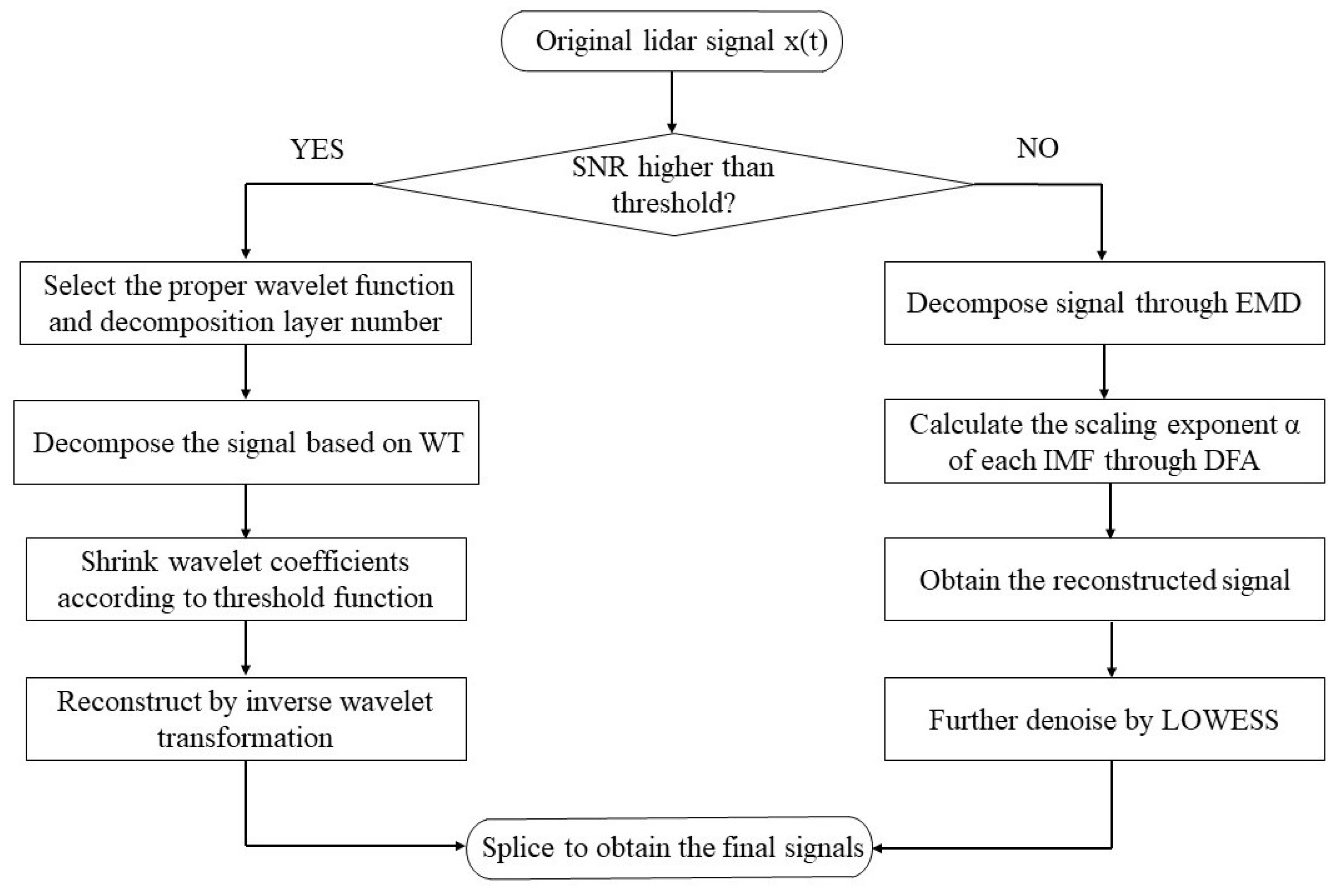
In engineering, the SNR of the lidar signal that needs to be processed often has a large dynamic range, and single denoising methods do not have good performance for the whole echo profile. So we plan to divide the signal to be processed into two parts according to the SNR and explore which method is more suitable in the case of integration time of 1200 s. The denoising performance of different algorithms, namely, moving averages (MA), wavelet hard thresholding (WTH), wavelet soft thresholding (WTS), EMD combined with DFA (EMD), EEMD combined with DFA (EEMD) and VMD combined with whale optimization algorithm (VMD-WOA) were compared for different evaluation indexes. As shown as

Table 2. Denoising performance with different heights for each algorithm.

Height Range/km	RAW	MA	WTH	WTS	EEMD	VMD-WOA
30–40	59.7109/1233.5	38.9091/1352.8	58.1694/1473.0	60.7532/1094.0	57.1453/1657.4	23.8776/7634.9
30–50	60.1029/837.7	34.2279/1647.4	60.9346/761.2	62.7611/616.8	56.6552/837.7	22.4360/6403.4
30–60	58.9623/780.6	32.1997/1700.4	59.1537/763.6	60.3729/663.6	55.7952/1124.0	22.4334/5234.4
30–70	59.2095/657.3	31.2823/1637.3	59.6589/624.2	61.2158/521.7	55.5927/996.8	22.4416/4530.8
40–70	42.6718/349.4	34.0989/937.5	44.6919/276.9	47.8397/192.7	47.2425/206.4	24.6075/2795.9
50–70	28.4629/297.1	35.5781/130.9	32.1896/193.4	35.8858/132.5	35.0250/139.6	26.3373/379.4
60–70	16.3705/282.9	26.1785/91.4	18.1742/229.8	20.8954/167.9	23.7415/121.1	26.1806/91.4

, the WT method could achieve better results when dealing with high SNR signal, while the decomposition algorithm had good performance when processing low SNR signal.

In order to make the algorithm as simple and efficient as possible on the basis of the above conclusions, we continued to explore the maximum height range that the WTS method can effectively denoise under the condition that the absolute error of density retrieval was less than 5% and the absolute error of temperature retrieval was less than ±10 K by the CH method [25]. The following paragraphs were also calculated under this condition. 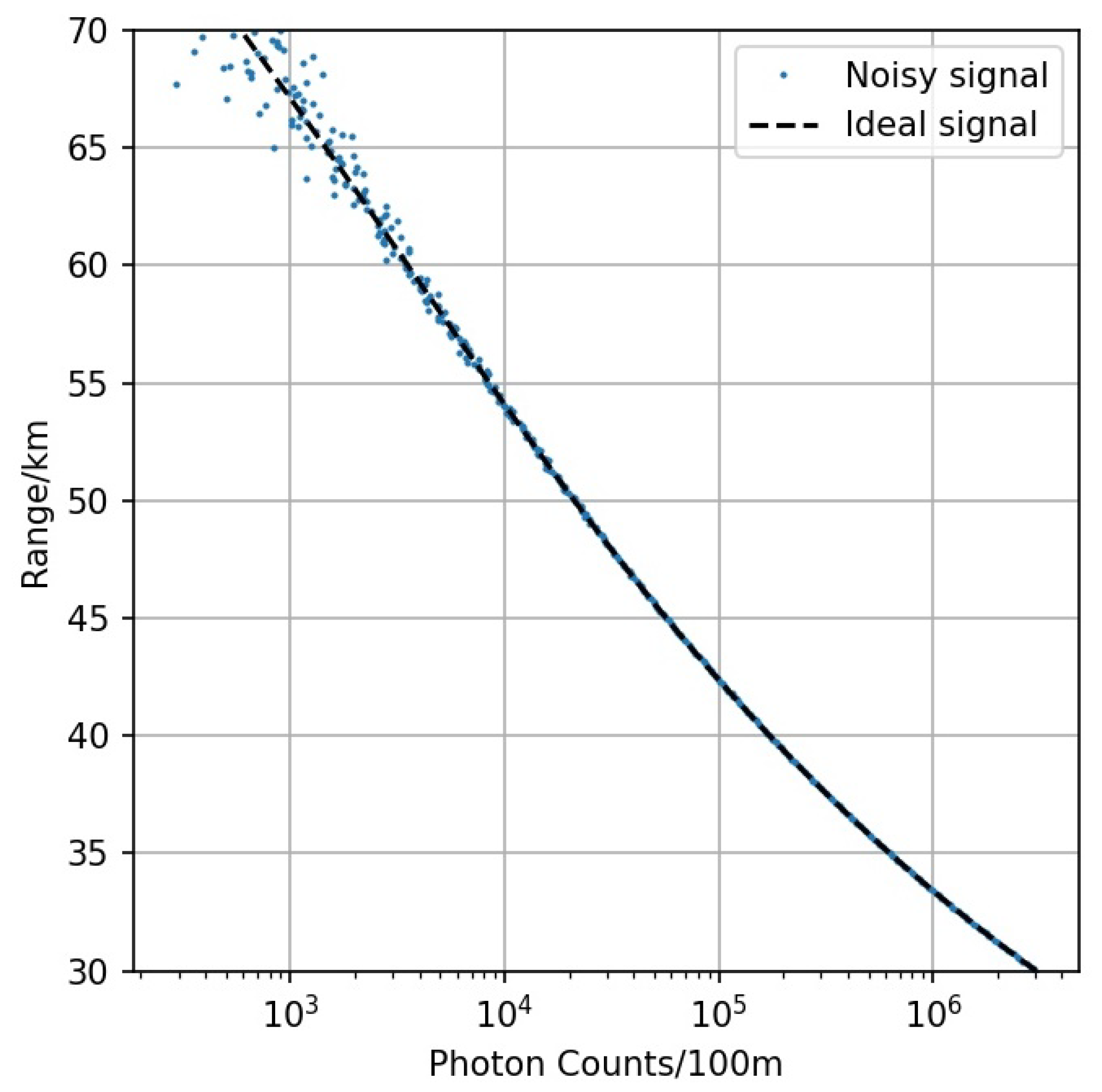Here, the WT method used the “$dB4$” wavelet basis and had three decomposition layers. Since the lidar echo signal obey Poisson distribution so that the signal are random, the mean value of the absolute errors of 100 profiles determined denoising performance of the following paragraphs. 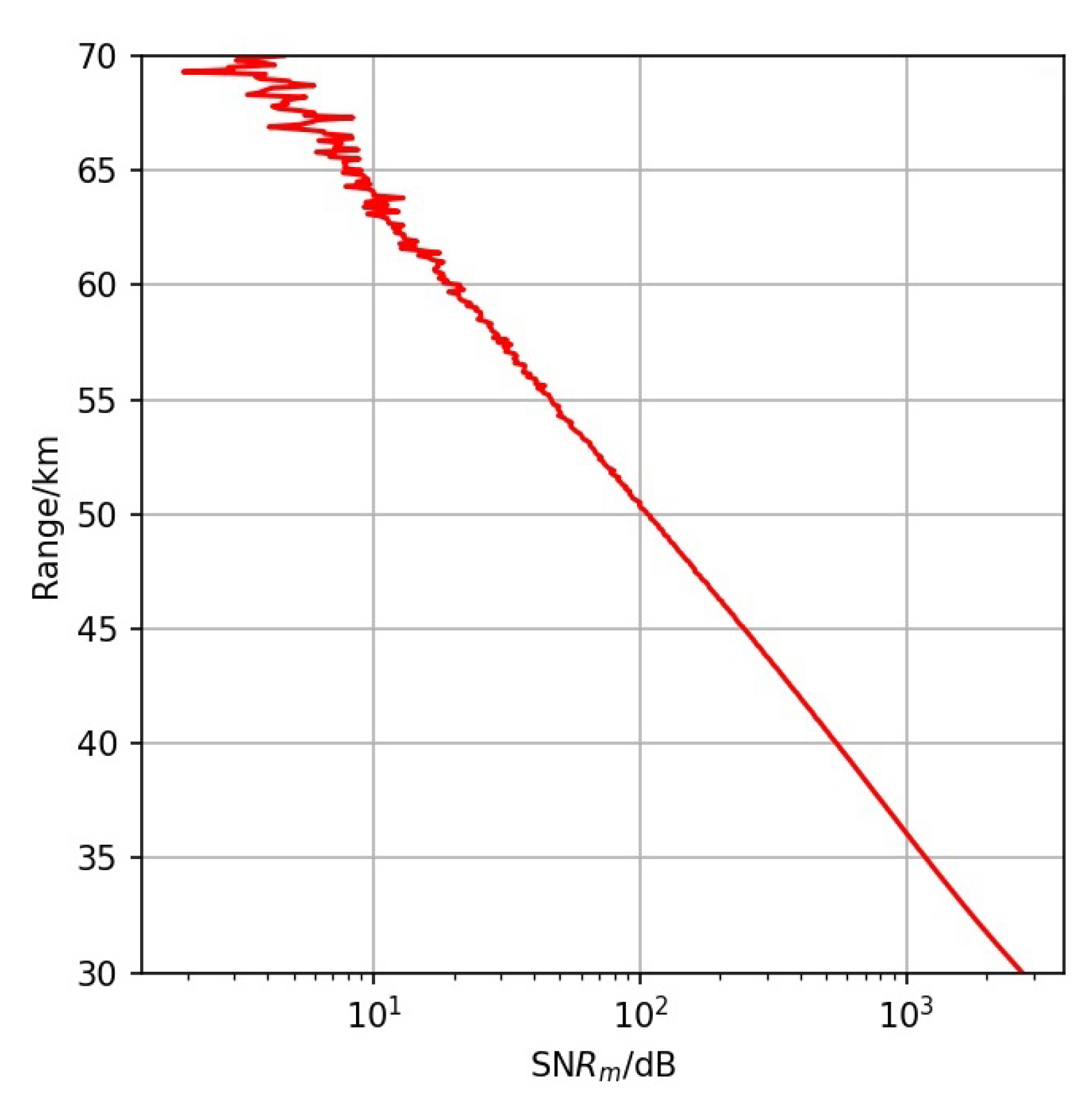As shown in Figure 4, when the maximum detection range was 59 km and the $SN{R}_m$ of the echo signal was generally above 16 dB, the WTS method could obtain valid data with the maximum absolute error of density retrieval of 1.02% and the maximum absolute error of temperature retrieval of 8.36 K.

It should be noted that the calculation of the SNR here is different from the previous one, due to the ideal signal not being able to be acquired in actual measurement. Considering the statistical properties of the detector, the SNR under Poisson distribution is defined as the ratio of the target backscatter echo signal to the square root of the original echo signal, where the original echo signal includes the target backscatter echo signal and the background noise. Usually, after a certain distance, the background counts of the lidar do not change with height, then it is considered that the photon counts collected by lidar is only the background noise. Thus, the average value of the photon counts after the certain distance can be taken as the background noise. The expression of $SN{R}_m$ is as follows:

$$SN{R}_m=\frac{P_{raw}\left(z\right)-BG}{\sqrt{P_{raw}\left(z\right)}}$$

(20)

where $P_{raw}\left(z\right)$ is the original echo signal and $BG$ is the background noise. Figure 5 shows the change $SN{R}_m$ with height.

Taking the simulated signal with the $SN{R}_m$ below 16 dB in Section 2 as an example, the DFA method was used to calculate the scaling exponent ${\alpha }_i$ of of each IMF for verification, and the results are given in

Table 3. The scaling exponent $\alpha$ of each IMF.

	$\mathit{IM}{\mathit{F}}_1$	$\mathit{IM}{\mathit{F}}_2$	$\mathit{IM}{\mathit{F}}_3$	$\mathit{IM}{\mathit{F}}_4$	$\mathit{IM}{\mathit{F}}_5$	$\mathit{IM}{\mathit{F}}_6$
$\alpha$	0.19	0.12	0.42	1.00	1.48	1.99

. Here, the length of non-overlapping windows was an eighth of the length of the input signal. The scaling exponent of $IM{F}_1-IM{F}_3$ were all less than 0.5, so they were considered as noise; The scaling exponent of $IM{F}_4-IM{F}_6$ were all higher than 0.5, so they were considered as signal.

For the purpose of validating the accuracy of the DFA method in distinguishing whether noise or signal was the main component of the IMFs, it was accumulated layer-by-layer from $IM{F}_2$ to $IM{F}_6$. Meanwhile, SNR and RMSE were calculated, respectively. Comparing the original signal with the accumulated signal shown in

Table 4. Denoising performance of layer-by-layer accumulating of IMFs.

	1–6 IMFs	2–6 IMFs	3–6 IMFs	4–6 IMFs	5–6 IMFs	6th IMF
SNR/dB	18.22	21.43	25.11	28.88	25.00	24.73
RMSE	286.97	198.32	129.87	84.11	131.53	135.67

, it was found that the accumulated signal of 4–6 layer IMFs was the closest to the original signal with the largest SNR and the smallest RMSE. This result is consistent with the results in Table 3, proving that the DFA method could be used as a reliable algorithm for qualification between noise and signal.

To explore which decomposition algorithm was more suitable for low $SN{R}_m$ signal, the EMD, EEMD, CEEMDAN, and VMD-WOA algorithms were selected for comparison. In the experiments with simulated signal, it was found that since the echo signals obey Poisson distribution and have a certain randomness, there was no method that always had the best denoising performance, which was also related to the selected SNR threshold. So as to solve this problem and find a generally suitable denoising method, the average SNR ($SN{R}_{ave}$) was used as the evaluation index to determine the denoising performance on the basis of multiple profiles. When selecting the signal with $SN{R}_m$ below 16 dB, after 100 statistics, the EEMD algorithm showed the best performance in 55 of them, and ranked first with 28.56 dB as shown in

Table 5. Denoising performance of different algorithms for low $SN{R}_m$ signals.

	RAW	EMD	EEMD	CEEMDAN	VMD-WOA
$SN{R}_{ave}$/dB	18.56	27.34	28.56	27.71	26.47
Best times		12	55	18	15

. For EEMD, the standard deviation of Gaussian white noise was 0.1, and Gaussian white noise was added 50 times.

Based on the above findings, we proposed to combine EEMD and LOWESS to achieve better denoising performance.

Table 6. Denoising performance of proposed algorithms compared with other methods.

	RAW	EEMD	EEMD-NLM	EEMD-WTS	EEMD-SVD	EEMD-LOWESS
SNR/dB	18.56	28.56	20.92	28.97	26.46	30.54

shows that the proposed EEMD-LOWESS outperformed all the other proposed methods [26] which could retain more effective signal. In addition, it was found that it was more effective at removing noise in low-frequency IMFs than extracting signal in high-frequency IMFs.

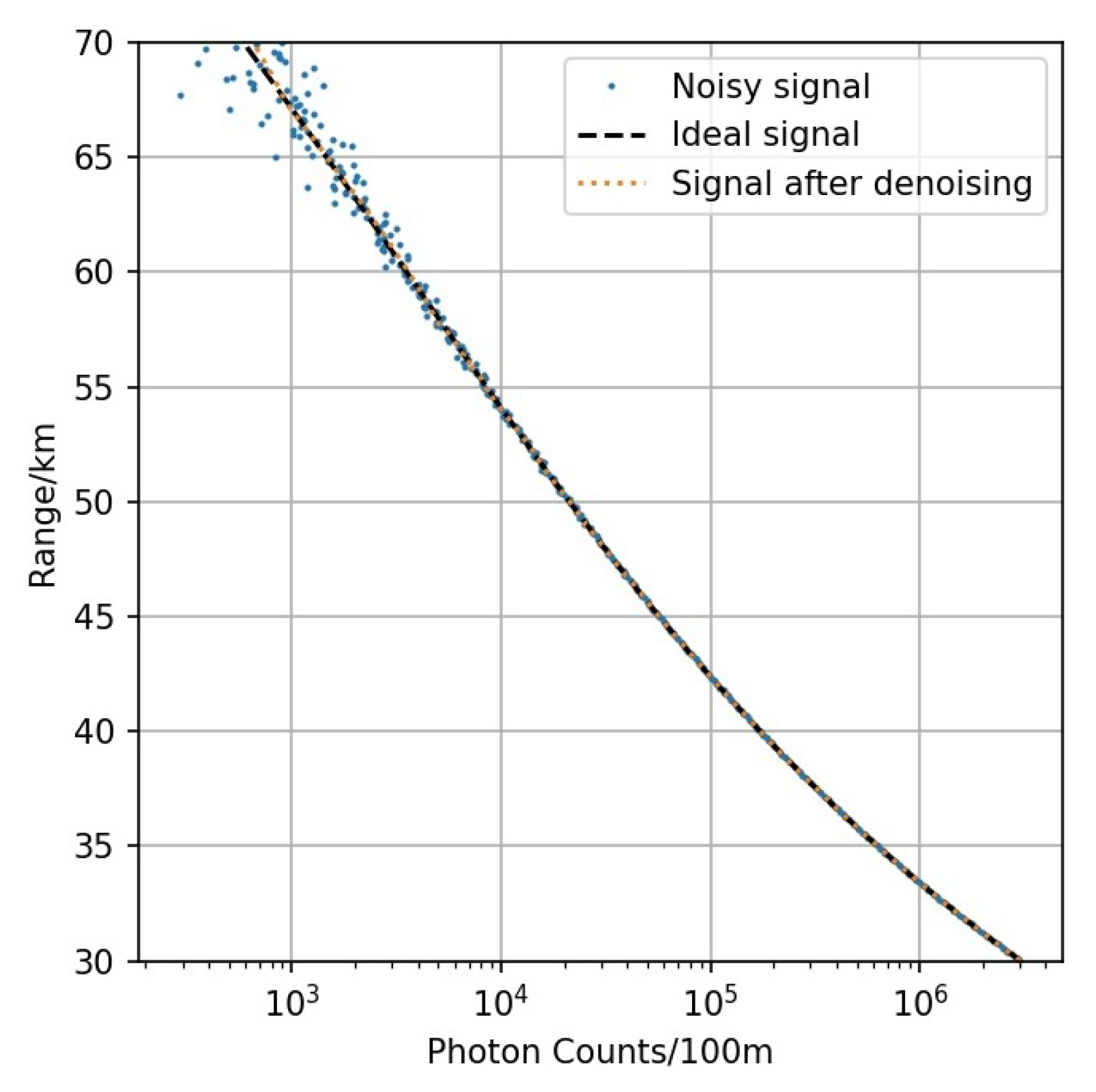
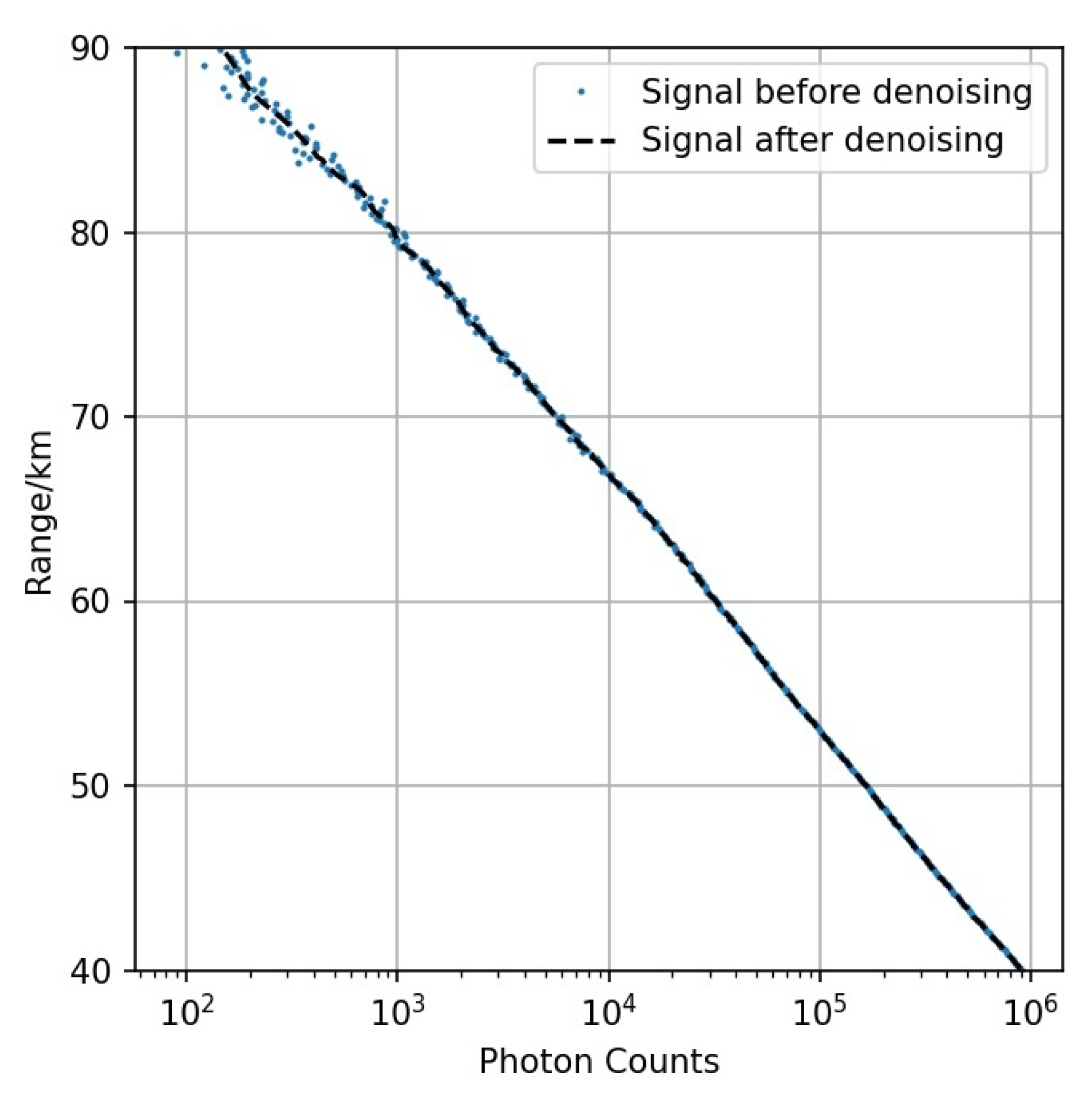
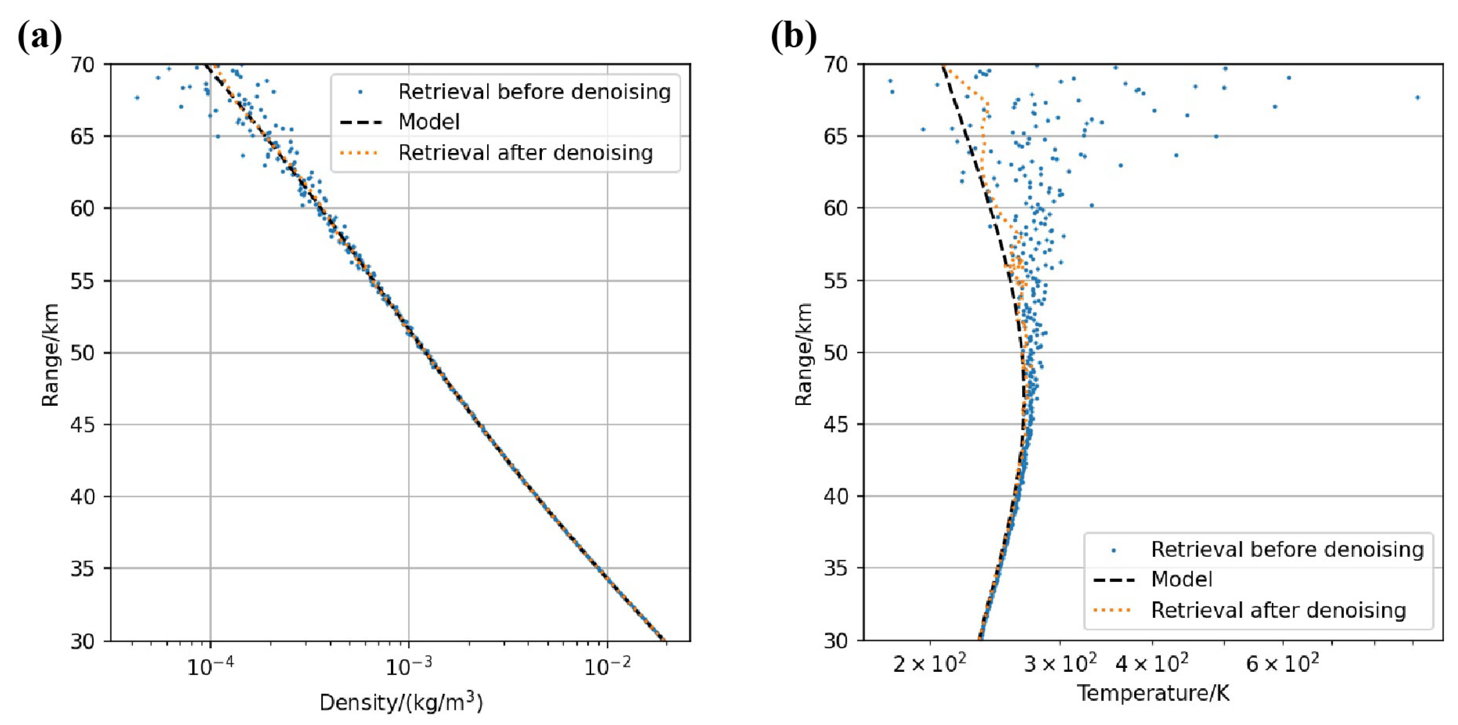
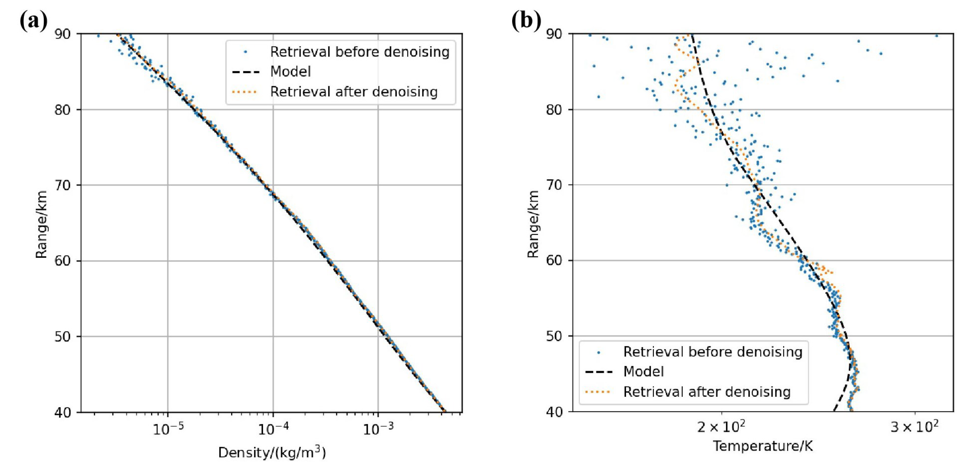
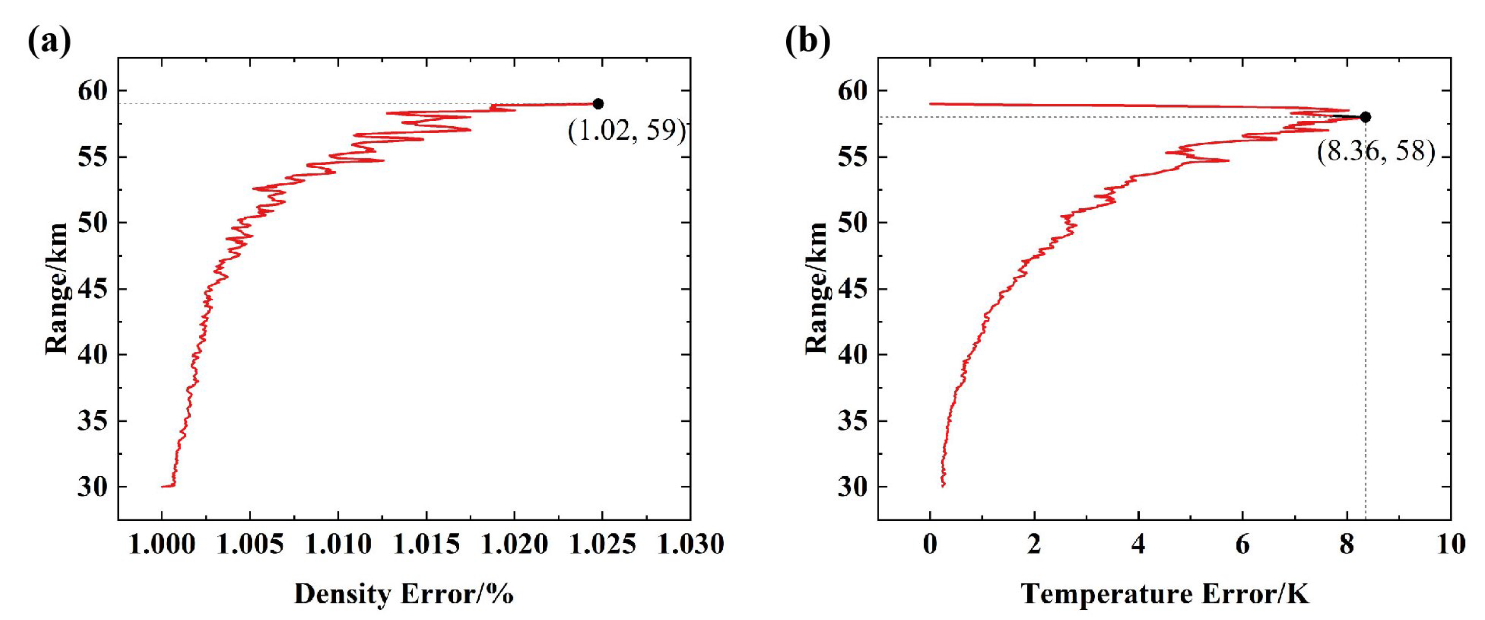
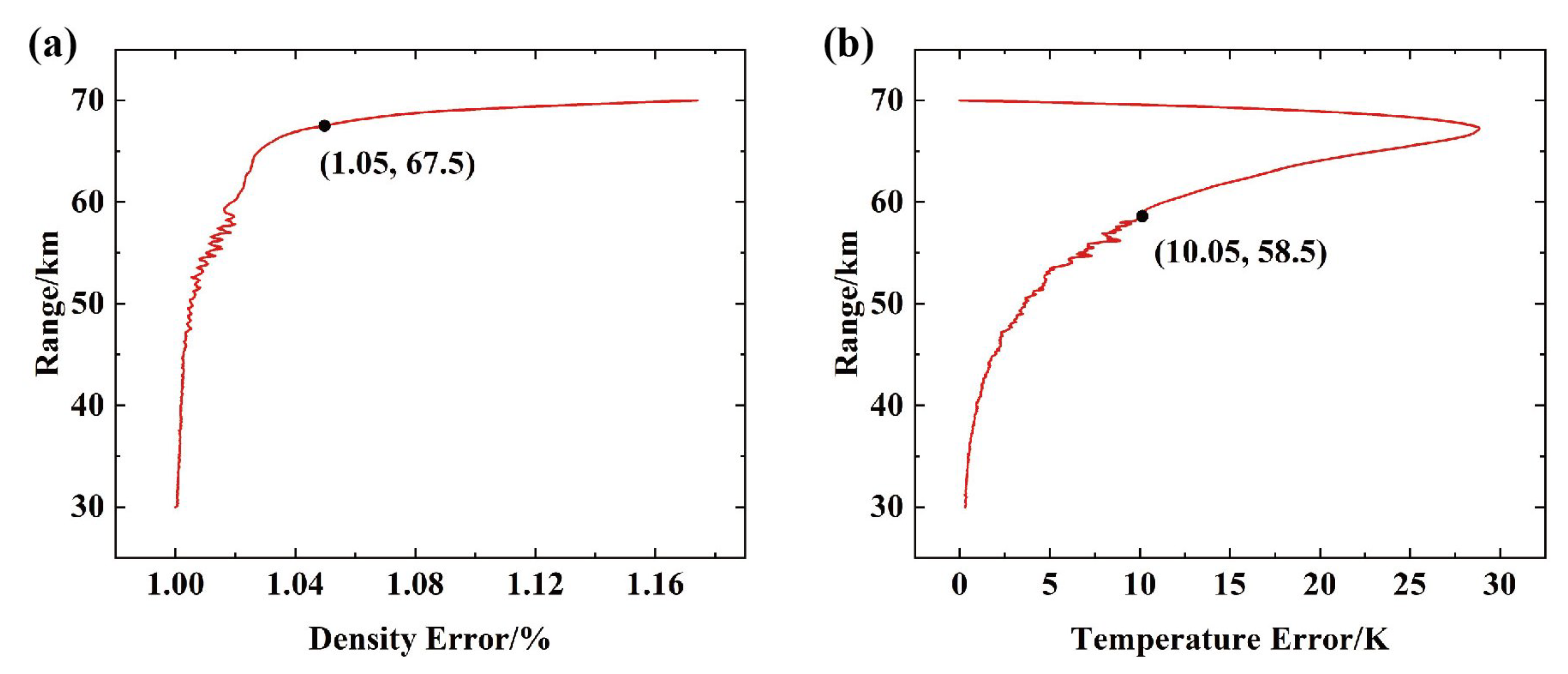
The denoising performance of the WT-EEMD-LOWESS algorithm is shown in Figure 6. The echo signals after denoising were smoother, more stable and closer to the ideal signal. The denoised data obtained through the above process were used as the input data of the CH method, and the density and temperature retrieval of the simulated signal could be gained, as presented in Figure 7a,b and then in contrast with the model temperature, the reliability of the proposed algorithm could be evaluated. It was not practical to calculate the absolute value of density due to several parameters fluctuating with measurement, so the relative density was calculated instead. As shown in Figure 8, under the condition that the error of density and temperature retrieval does not exceed 5% and 10 K, the maximum detection range was 67.5 km and 58.4 km after denoising, which were 12.8 km and 11.1 km higher than those without denoising, respectively.

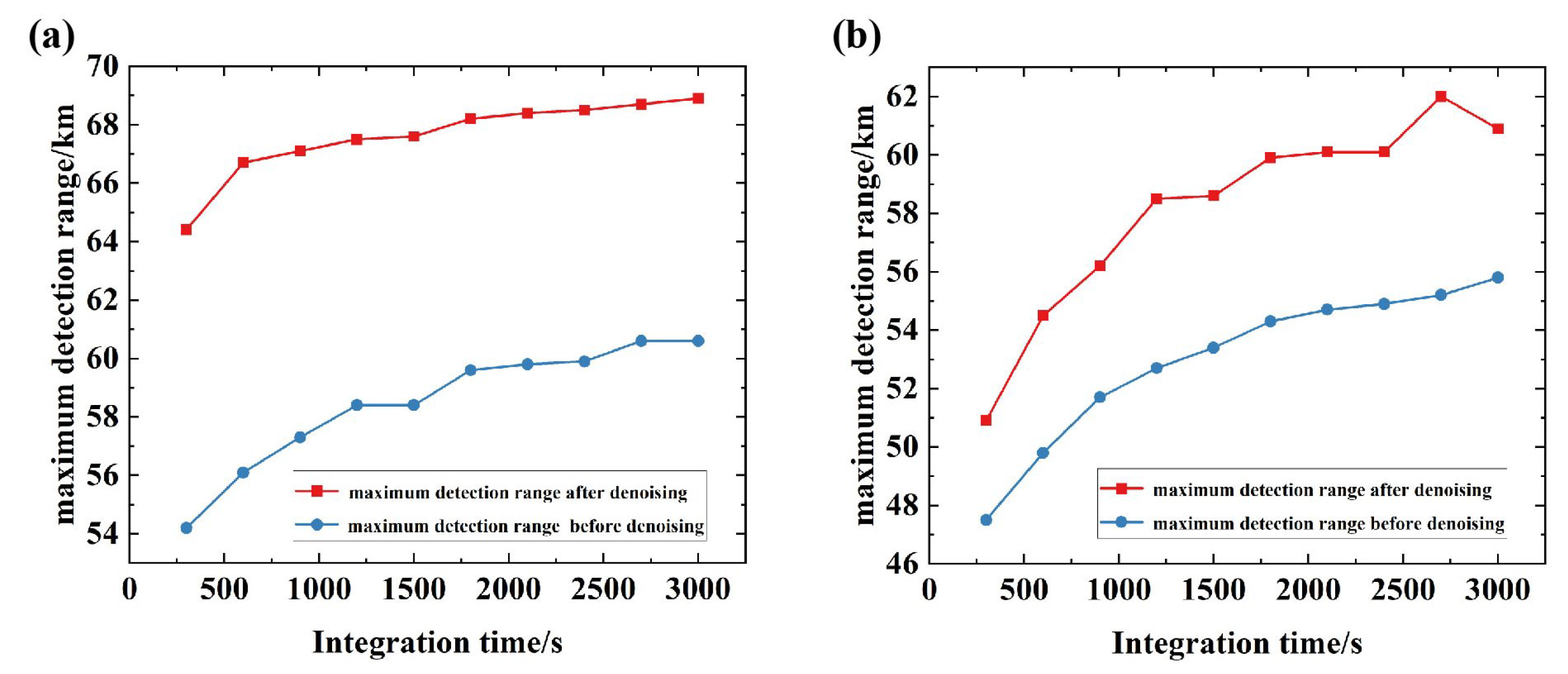
Futhermore, the algorithm was applied to simulated the lidar echo signal with integration times of 300–3000 s. The variation of the maximum detection range with the integration time is shown in Figure 9. It could be found that the maximum detection range increased with the accumulation of the integration time, which was conformed to the law. When the error of density retrieval was less than $5\%$, the maximum detection range increased first fast and then slowly with the integration time. The reason is that when the integration time was too long, the detection range was close to the limit of 70 km. The maximum detection range changed slowly with the integration time at 60 km when the error of temperature retrievals was less than 10 K. The reason is that the measurement was inaccurate within 10 km below the seed temperature, which is an inherent shortcoming of the CH method.

4.2. Real Experiment on a Lidar Echo Signal

In order to further investigate the denoising performance of the algorithm proposed in this paper, we used the measurement data provided by the National Space Science Center, CAS. The signal was obtained by continuously observing the atmosphere at 40${}^{\circ }$18${}^{\prime }$N latitude and 116${}^{\circ }$40${}^{\prime }$E longitude by ground-based lidar and the parameters of lidar system are shown in

Table 7. Ground-based lidar system.

System Parameter	Value
Laser pulse energy/mJ	500
Telescope diameter/m	1
Average power/W	>10
Wavelength/nm	532
Pulse width/ns	8
Quantum efficiency	0.4
Filter transmittance	0.8
System optical efficiency	0.02
Pulse repetition frequency/Hz	30
Degree from zenith/°	0

below. The observation time was 3 September 2018, 17:30. The measurement results and denoising performance are shown in Figure 10.

Based on the denoised echo signal, the density and temperature retrievals of the measured data can be obtained by the CH method, as shown in Figure 11. The maximum error between density retrieval and model was reduced from $1.36\%$ to $1.1\%$, and the maximum error of temperature retrieval and model was reduced from 125.79 K to 13.84 K. The improvement of the maximum detection distance was not obvious with error of density and temperature retrievals less than $5\%$ and $10$ K separately, due to the fact that the measured original signal is different from the model when the SNR is high. It can also be seen that when the SNR is low, the performance improvement of the proposed algorithm is more obvious, and when the SNR is high, the discrepancy between the retrievals and model depends more on the original data itself.

5. Conclusions

Based on WT and EEMD, a new WT-EEMD-LOWESS denoising method for signal with large SNR dynamic range was proposed by using the simulated lidar signal. The echo signal was divided into two parts with SNR of 16 dB as the boundary. The high SNR part was denoised by the WT method; the low SNR part was decomposed by the EEMD algorithm first, and the scaling exponent $\alpha$ of each IMF was calculated by DFA, then the IMF with $\alpha >0.5$ was used to obtain the reconstructed signal. The reconstructed signal still contained noise, so the LOWESS method was performed on the reconstructed signal to futher extract the signal. Moreover, in order to verify the effectiveness of the algorithm, the simulated denoised signal with a typical integration time of 1200 s was used as the input data of the CH method for density and temperature retrievals. In the case that the absolute error of density retrieval was less than $5\%$ and the absolute error of temperature retrieval was less than $5$ K, the maximum detection range improved 12.8 km and 11.1 km, respectively. This algorithm was also verified to be effective with an integration time of 300–3000 s. In addition, the WT-EEMD-LOWESS method was applied to the measured lidar echo signal. The experimental results showed that the algorithm achieved a good denoising performance in the low SNR signal part on the basis of not distorting the signal. The maximum density error was reduced from 1.36% to 1.1% and the maximum temperature error was reduced from 125.79 K to 13.84 K which indicated that the proposed algorithm has good application value in Rayleigh scattering lidar signal processing.