Influence of Assimilating Wind Profiling Radar Observations in Distinct Dynamic Instability Regions on the Analysis and Forecast of an Extreme Rainstorm Event in Southern China

Abstract

This study quantitatively examines the contribution of assimilating observations in the regions with different dynamic instabilities to the analysis and prediction of an extreme rainstorm event in Fujian Province of China. The wind profiling radar (WPR) observations are classified into two groups, i.e., strong and weak instability areas (SIA and WIA), according to their local dynamic instability identified by the ensemble spread. Their performance of assimilation and prediction in terms of the wind and precipitation are evaluated and compared in detail. The results show that the wind analysis error by assimilating all of the WPR observations can be reduced by about 30%. In particular, the wind analysis errors by only assimilating the observations in the SIA are about 12% lower than those in the WIA. They are related to the existence of the low-level horizontal wind shear with strong instability in the SIA. The case study shows that the assimilation of observations in the SIA can effectively correct the wind fields on the two sides of the wind shear line, producing an improved precipitation forecast compared to observation assimilation in the WIA.

1. Introduction

The skill of numerical weather prediction (NWP) crucially relies on the accuracy of the initial condition (or analysis) that is generated by the data assimilation (DA) procedure [1,2,3,4,5]. A typical DA algorithm exists to optimally estimate the state of the real atmosphere by combining the short-range model forecast (i.e., the first guess field, denoted by FG hereafter) and the observations that measure the real atmosphere [6,7]. Therefore, the accuracy of the initial analyses is driven by multiple factors, such as the model performance and the observational precision. One of the most important factors is the model’s instability against the real atmosphere, which varies in space and time. Such model instabilities are closely related to the weather systems and regimes. For example, the flow in the front of an upper-troposphere trough usually has stronger baroclinic instability than its tail part. The regions with stronger instability generally have larger forecast uncertainties (or errors) of the FG fields and thus correspond to a less accurate analysis than those dynamically more stable regions [8,9].

It has long been conceived that NWP will benefit from supplementary observations deployed in critical regions, that extend the conventional observational network [10,11]. The critical regions are generally referred to as the regions that have the strongest instability or the fastest unstable growth of forecast errors [12,13,14]. The impact of assimilating observations in the critical regions has been extensively studied, but mostly in observing system simulation experiments (OSSE) [15,16,17,18].

Wind profiling radar (WPR) is a useful meteorological observation device that collects temporally continuous vertical-profile observations of the horizontal wind vectors above the ground [19]. This type of observation provides critical information on the circulations from lower to upper levels associated with mesoscale weather systems, such as the local wind shear and low-level jet [20,21,22]. Many studies have confirmed the positive influence of WPR data on the mesoscale numerical prediction [23,24,25,26], especially on the short-range temporal scale in the range of 0–12 h [22,27,28]. In the operational observing network over southern China, the WPR has a wide coverage at a horizontal resolution of about 70 km and a vertical resolution of approximately 150 m. The maximum vertical altitude of the WPR observations can reach 8–14 km. They provide valuable observations of the main weather systems in southern China, especially the circulation systems at various elevations associated with the high-impact heavy rainstorms that frequently occur in this region. The WPR observations are an effective supplement to the existing conventional observing network especially at the mid and upper levels in southern China. Although the assimilation of the WPR observations and their impact on the prediction of local rainstorms in southern China have been studied in various studies [21,22,29], the relative importance of the observations in the different regions in contributing to the forecast skill relating to rainstorms has not been investigated and quantitatively compared. In particular, a heavy rainstorm in southern China is often induced by a complex interaction of multi-scale systems with different dynamic instabilities. A quantitative comparison of the assimilation impact of the WPR observations in different regions with the spatially varying dynamic instability is key to understanding the influences of the different weather systems on the rainstorms in southern China and augmenting and upgrading the existing observing network.

The ensemble forecasts are a series of model integrations starting from initially close conditions, offering a sample of the possible future states. The spread of ensemble forecasts is often used to quantify the forecast uncertainties, which are closely related to the dynamic instability associated with weather systems [30,31,32,33]. The regions with a larger ensemble spread generally indicate the existence of probably more unstable weather regimes. The goal of this study is to quantitatively compare the impact of assimilating the WPR observations in strong instability areas (SIA) and weak instability areas (WIA) on the prediction of a local rainstorm in the Fujian Province of southern China. The ensemble forecast spread is used to approximately identify the spatial instability. The WPR observations are accordingly divided into those in the SIA and WIA. Their separate and combined assimilation effects on the prediction of a local rainstorm are comprehensively evaluated and compared. The relevant mechanisms are also analyzed and clarified by relating the SIA and WIA to the corresponding weather systems.

This study is arranged as follows. Section 2 briefly describes the weather case and introduces the model configuration, the observational data, and experimental design. In Section 3, the assimilation impacts of the WPR data on the SIA, WIA, and their combined areas on the initial analysis and forecast, are evaluated and compared. The relevant mechanisms are diagnosed and examined in detail. Finally, the summary and conclusions are given in Section 4.

2. Weather Cases, Model, and Experimental Design

2.1. Weather Cases

An extreme heavy rainstorm event occurred in Fujian Province (highlighted in blue in Figure 1), southern China, during the period from 14 to 17 May 2019. The observed 24-h accumulated rainfall in Sanming city, near the center of Fujian Province, reached 300 mm on 16 May, which broke the historical record of local daily precipitation since 1961. Most of the operational global NWP systems showed limited forecast skills on the location and intensity of the precipitation. For example, the maximum 24-h precipitation in a 36-h forecast provided by the European Centre for Medium-Range Weather Forecasts (ECMWF) was located in the northwest of Jiangxi Province, about 300 km far away from the observed precipitation center. Moreover, the forecasted maximum 24-h precipitation was less than 100 mm, failing to give a timely warning of the extreme heavy rainstorm. The initial ensemble spread of the global ensemble forecasts at the National Centers for Environmental Prediction (NCEP) presented large amplitudes near the precipitation regions (see Figure 2), implying possibly higher uncertainties of the initial analysis in these regions than in other regions. Given the obvious spatial differences in the initial uncertainties in distinct regions, this study will perform hindcast experiments to evaluate the impact of assimilating the observations in these regions into the analysis and prediction of the rainstorm event.

2.2. Model Configuration and Data Assimilation System

The hindcast experiments were carried out using the Weather Research and Forecasting (WRF) Model version 3.7. The WRF model is a fully compressible non-hydrostatic model using a terrain-following hydrostatic pressure vertical coordinate and adopting the Arakawa C-grid as the gird staggering [34], which is widely used in mesoscale synoptic analysis research. The model configuration uses a two-way nested domain grid (Figure 1) with a horizontal resolution of 18 km for the parent domain (D01), and 6 km for the inner domain (D02). Both of the domains have 53 vertical levels. D01 covers the East Asia region with a mesh of 141 × 131, and D02 covers southern China with a mesh of 241 × 241. The physical parameterizations used in this study include the WRF single-moment five class microphysics scheme [35], the rapid radiative transfer model longwave radiation scheme [36], the Goddard shortwave radiation scheme [37], the Grell 3D cumulus parameterization scheme [38], and the MYJ planetary boundary layer scheme [39]. The lateral boundary conditions for the background fields of DA and the model free forecasts were provided by the 0.5 × 0.5 operational global forecasts of the global forecast system (GFS) at NCEP.

The DA system in this study used the three-dimensional variational (3DVAR) DA scheme [40], with a 1-h time window for the assimilation of observations. The static background error covariance was generated using the typical National Meteorological Center (NMC) method [41]. The WPR observations (red dots) were collected by the China Meteorological Administration (CMA) and covered the coastal provinces, including Jiangsu, Shanghai, Zhejiang, Jiangxi, Fujian, and Guangdong from eastern China to southern China (Figure 1) at a spatial resolution of nearly 70 km. The observational errors of WPR below 500 m were relatively larger than at the upper levels, due to the surface friction effect. On the other hand, WPR is a remote sensing observation device; thus, the attenuation of the remote sensing signals caused by heavy rain may affect the accuracy. These WPR observations were assimilated only for the inner domain (D02). The surface automatic weather station (AWS) observations (black dots in Figure 1) were used for the independent verification of the forecast skill, and thus not assimilated to the initial conditions. Due to the high vertical resolution of the WPR data at approximately 150 m, they were preprocessed by a typical thinning step to better match the model vertical resolution [22,29]. In the thinning step, the WPR observations that were closest to each model vertical level were selected, while the rest of the data were rejected, which means the observations after the thinning had a similar vertical resolution with the model.

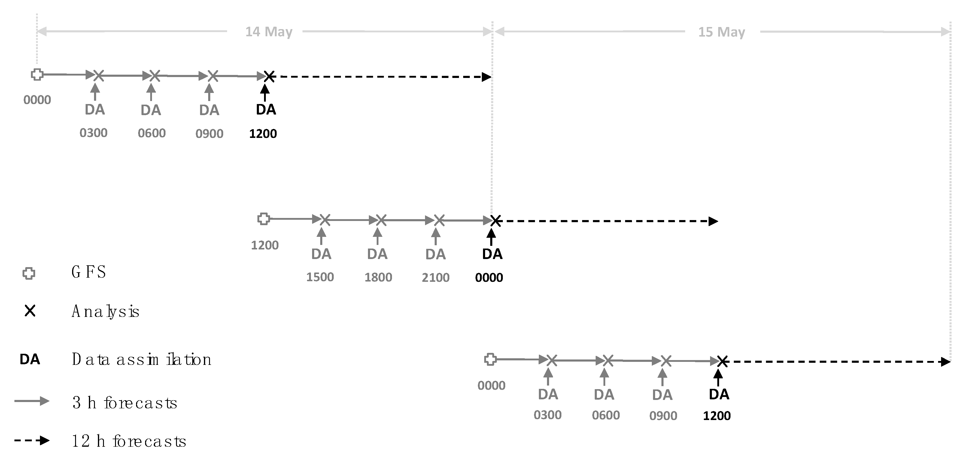
2.3. Experimental Design and Evaluation

The numerical experiments in this study were conducted in a cycling DA and prediction system, based on the 3DVAR scheme (Figure 3). Given the first case as an example, the first DA cycle at 0000 UTC on 14 May was activated with a cold start, using initial and boundary conditions downscaled from the analysis field of the GFS product at NCEP. The WPR observations were then assimilated to generate the high-resolution analysis in the first DA cycle. Afterward, the assimilation step was performed every 3 h in continuous cycles, with the 3-h WRF model forecast initialized from the previous analysis as the FG. To reduce the influence of the model spin-up on evaluation, the first three DA cycles were eliminated. The analysis of the fourth DA cycle at 1200 UTC on 14 May was used to initialize a 12-h forecast at a one-hour output frequency for evaluation. This entire process was repeated six times every 12 h to produce a total number of six cases at an interval of 12 h. Such a design of the experiment can reduce the dependence of the forecast cases and mitigate the possible drift of continuously cycled analyses from the truth.

As pointed out in Section 1, the goal of this study is to compare the assimilation impact of the WPR observations located in regions with different dynamic instabilities. The regional instability is approximately quantified using the ensemble spread of the initial ensemble members from the global ensemble forecast system at NCEP (downloaded from https://apps.ecmwf.int/datasets/data/tigge/levtype=pl/type=cf/, (accessed on 9 July 2019)) before the assimilation of observations. The use of the same prediction system (i.e., NCEP) to calculate the spread can provide a relatively consistent identification of the regional stability in the FG, avoiding the possible bias of numerical results. The procedures to divide the SIA and WIA according to the spatial distribution of ensemble spread can be seen in Section 3.1. Three DA experiments were implemented and compared in this study. “E_SIA” and “E_WIA” are the DA experiments that only assimilated the WPR observations in the SIA and WIA in D02, respectively. The experiment that assimilates all of the WPR observations was also carried out (termed as “E_ALL”).

The analysis and forecast of zonal (U) and meridional (V) winds at different levels were evaluated by verifying them against the WPR wind profile observations, because there were very limited observations available for the verification of the mid-and upper-level wind fields. There were only three sites for radiosonde observations in the core region, i.e., Fujian Province, at which the radiosondes were launched only twice a day. These observations were too sparse for the verification of the wind fields. The popular metric, root mean square error (RMSE), was calculated to assess the performance of wind (U and V components) analysis and forecast, which was defined as follows:

$$RMSE=\sqrt{\frac{1}{N}{{\displaystyle \sum }}_{i=1}^N{\left({\mathrm{M}}_i-{\mathrm{O}}_i\right)}^2},$$

(1)

where N is the number of WPR observations within D02; ${\mathrm{M}}_i$ represents the analysis and model forecast interpolated in the observation space; and ${\mathrm{O}}_i$ is the corresponding observation.

The forecast of the surface precipitation was verified against the AWS observations. Two widely used metrics, the Threat Score (TS) and the Bias Score (BIAS), were computed to evaluate the skill of the precipitation forecast:

$$TS=\frac{C}{F+NO-C},$$

(2)

where F represents the number of forecasted precipitation events; NO is the number of observed precipitation events; and C is the number of the events with correctly forecasted precipitation, i.e., the observed and forecasted precipitation events occur together. The range of TS is 0 to 1, with a larger value indicating a more skillful precipitation forecast. The BIAS is defined as:

$$BIAS=\frac{F}{NO}$$

(3)

BIAS varies from 0 to positive infinity, with a value less or greater than 1 indicating an underestimation or overestimation of the precipitation.

3. Results

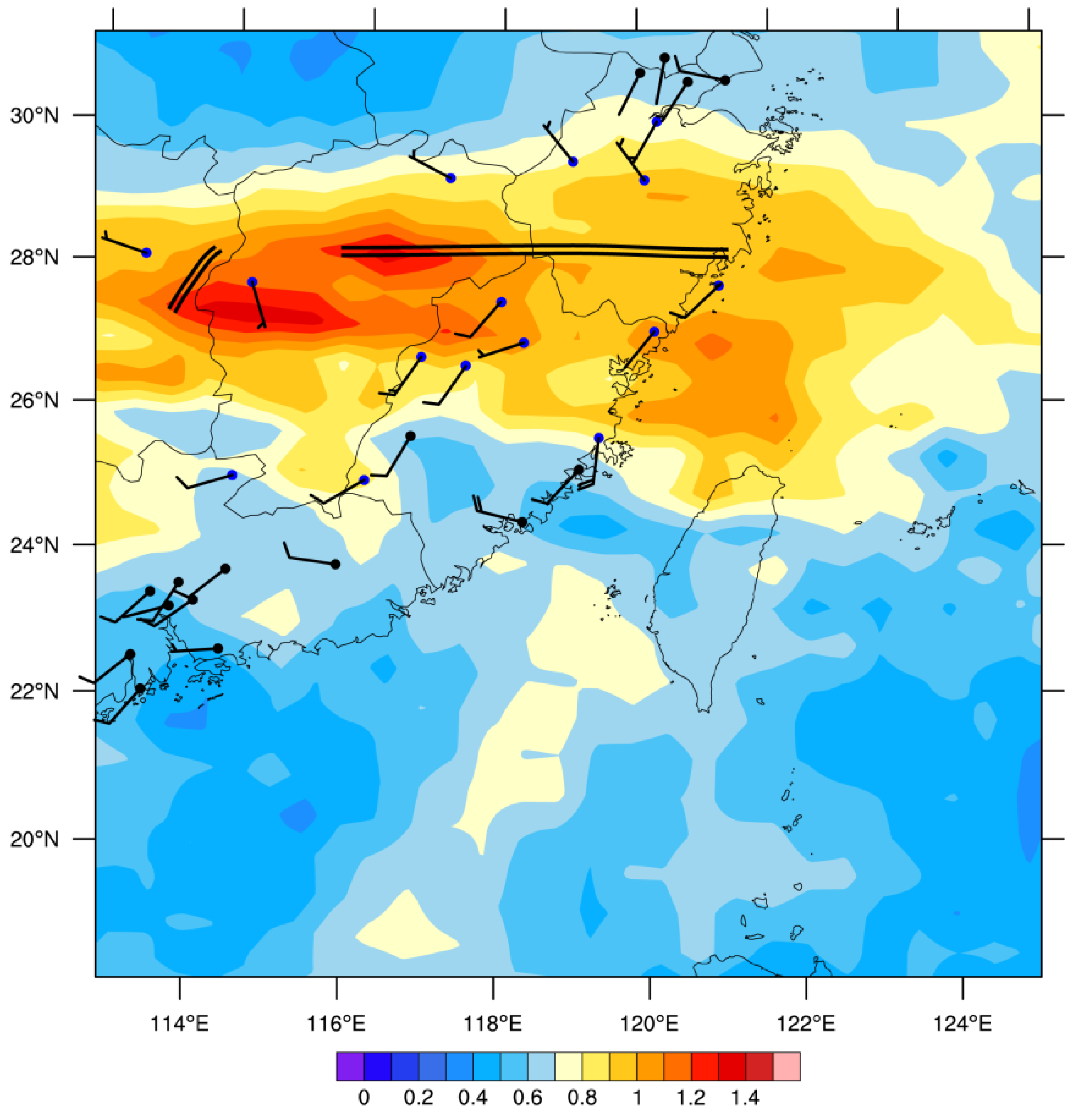
3.1. Spatial Instability

The spatial distribution of the initial ensemble spread (shaded) of the kinetic energy averaged over three vertical levels (850, 500, and 200 hPa) at 1200 UTC on 15 May 2019 is shown in Figure 2. The kinetic energy is calculated by (u² + v²)/2, where u and v represent the zonal and meridional wind components, respectively. Noticeably, there is a high-spread band between $26$–${29}^{°}$ N extending from the west of Jiangxi Province to the east China sea zonally, with the maximum in the west and north of Jiangxi Province. This high-spread band is probably associated with the strong instability caused by the horizontal wind shear along nearly ${28}^{°}$ N (highlighted by black parallel lines). The wind shear line is a convergence zone between the cold and dry northwesterly wind and the warm and wet southwesterly wind, as illustrated by the WPR wind observations at 850 hPa. The mesoscale synoptic circulation confirms the validity of using the initial ensemble spread in identifying the spatial dynamic instability. The WPR observations at individual levels are reordered, according to the value of the ensemble spread of the kinetic energy at the observation location, from the most unstable to the most stable. The first half of the WPR observations (i.e., 50% percentile) are categorized into the SIA group and are assimilated in the experiment E_SIA, while the second half belongs to the WIA group and is assimilated in the experiment E_WIA.

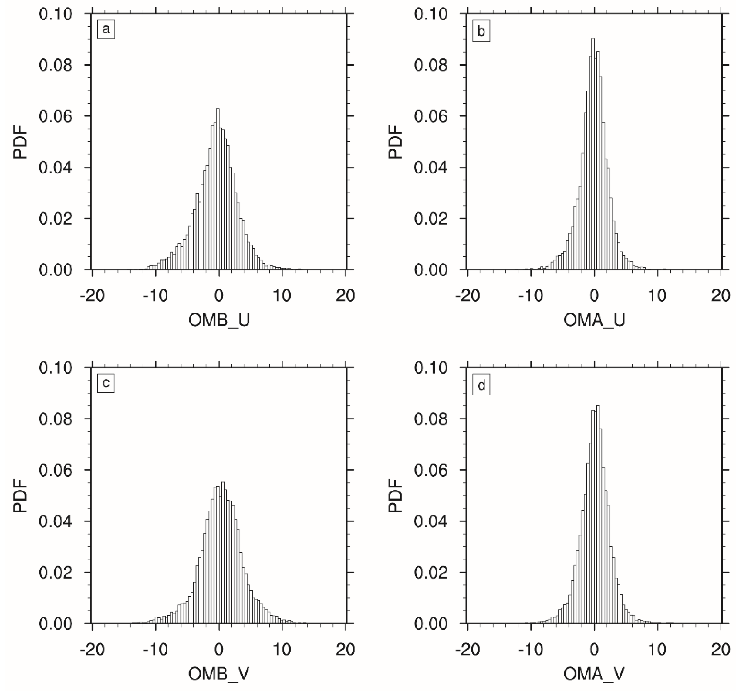
3.2. Impact of Assimilating WPR Data on Initial Analysis

An effective DA system can ingest the observational information into the analysis. The analysis with the assimilated observations would thereby have better fitting with the observations than the background. The fitting between the WPR observations (“O”) and background (“B”) averaged over all of the cases was assessed (i.e., observational innovation) first for the SIA, WIA, and the entire region (

Table 1. The observational innovation between the WPR observations (“O”) and background (“B”) averaged over all cases in the SIA, WIA, and entire region for zonal (U, units: m s⁻¹) and meridional wind (V, units: m s⁻¹).

	Absolute Error		Standard Deviation
	U	V	U	V
SIA	2.68	2.97	2.78	2.95
WIA	2.36	2.42	2.51	2.53

). The mean absolute observational innovation (i.e., |O−B|) in the SIA was about 11% and 20% higher than that in the WIA for the U and V winds, respectively. The absolute observational innovation in the SIA also had a larger variability (i.e., standard deviation) than in the WIA. These results suggest that the FG has larger uncertainties in regions with more unstable dynamics (i.e., SIA). Figure 4 further compares the fitting of the WPR observations at all of the altitudes in all of the cases with the corresponding background (i.e., O vs. B) and analysis (i.e., O vs. A) interpolated in the observation space for U and V. The analyses of both U and V presented a better fitting with the observations than the background (cf. left and right panel in Figure 4). Quantitatively, |O−A| averaged over all of the altitudes and all six cases were significantly lower than |O−B| by about 30% (1.6674 vs. 2.5069 m s⁻¹ for U and 1.7407 vs. 2.6029 m s⁻¹ for V). These results signify the effective assimilation of the WPR observations in modulating the wind analysis fields.

The probability density functions (PDF) of O−B and O−A for U and V winds for all of the levels and all of the cases are further displayed in Figure 5. It can be seen that the PDF of both O−B and O−A for U and V present a Gaussian-like distribution with a near-zero mean, indicating that the fitting of both the analysis and background is statistically unbiased. Moreover, the standard deviation of O−A is clearly smaller than that of O−B for both U (2.25 vs. 3.28 m s⁻¹) and V (2.32 vs. 3.41 m s⁻¹), implying a better fitting of the analysis to the observations than the background, as suggested by Figure 4.

To quantify the contribution to the initial analysis of assimilating the WPR observations into the SIA and WIA, Figure 6 compares the horizontal root mean square |O−B| (green) and |O−A| in the E_SIA (blue), E_WIA (red), and E_ALL (orange) experiments at the different levels for U (a) and V (b) at 1200 UTC, 15 May 2019. |O−A| in E_ALL is smaller than |O−B| at all of the vertical levels for U and their differences are overall homogeneous vertically at about 1 m/s (Figure 6a). This is predominantly contributed by the assimilation of the observations in the SIA, except for the near-surface level and the upper troposphere. It is because the SIA, with more intense instability, has a larger FG error variance (Table 1), and thus has a greater weight on the WPR observations in the assimilation. In contrast, the differences between |O−A| in E_ALL and |O−B| for V are distinct at the different levels, which are much larger in the upper and lower troposphere than in the mid-troposphere. The limited assimilation impact in the mid-troposphere is possibly associated with the relatively high-skill simulation of the mesoscale circulation in the FG at this level, corresponding to the minimum |O−B| of FG across the levels (see the green line in Figure 6b). The averaged results over all of the cases and all of the altitudes show that the assimilation of the WPR observations in the SIA (i.e., E_SIA) can attain around a 60% error reduction in the analysis error in E_ALL, relative to the FG error, while E_WIA can attain only a 30% error reduction (not shown).

3.3. Impact of WPR Data on the Forecast

This section verifies the forecast skill of the E_ALL, E_SIA, and E_WIA experiments in D02. Figure 7 shows the sample-mean RMSE of the 850-hPa wind forecasts verified against the WPR observations. At the initial time, E_ALL has the smallest RMSE for both U and V, followed by E_SIA and E_WIA, as suggested by Figure 6. The wind analysis error of E_SIA is about 12% lower than that of E_WIA for both U and V. The F-test shows that the 12% reduction in wind analysis error is statistically significant at a 90% and 99% confidence level for U and V, respectively. Interestingly, despite the larger analysis error of U and V winds, E_SIA has a very close RMSE of the U and V forecasts compared to E_ALL at 6 and 12 h. It possibly implies that the baroclinic instability associated with the horizontal wind shear plays a critical role in modulating the evolution of the circulation. Significantly reducing the initial errors in these regions (i.e., the SIA) may benefit the subsequent wind forecasts to the largest extent. E_WIA, with the worst accuracy of initial condition, performs much worse than E_ALL and E_SIA in the wind forecasts (about a 10% increase in the RMSE averaged over time). The lower mean error for V wind at 12 h than at 6 h in Figure 7 is possibly an effect of the diurnal variation (not shown).

The averaged TS and bias over all of the six cases are evaluated for E_ALL, E_SIA, and E_WIA in Figure 8 for the prediction of the first 3-, 6-, 9-, and 12-h accumulated precipitation greater than 0.01 and 15 mm. E_SIA displays the best TS of the rainfall forecasts for all of the lead times, followed by E_ALL and E_WIA. E_ALL performs better than E_WIA, especially in the TS with the 0.1-mm threshold (Figure 8a), but performs overall similarly to E_WIA for the 15-mm threshold (Figure 8b). The maximum relative improvement of TS for E_SIA relative to E_WIA reaches about 6% and 19% for the thresholds of 0.1 and 15 mm, respectively, at 6 h. These results further indicate that the assimilation of the observations within the regions with unstable weather dynamics possibly plays the most important role in improving the precipitation forecast. In contrast, E_ALL, E_WIA, and E_SIA present little differences in the performance of the BIAS score. It possibly implies that the assimilation of only the momentum observations, without considering thermodynamic observations such as water vapor, has little influence on the prediction of the precipitation area (i.e., the BIAS).

3.4. Sensitivity of the Selection of WPR Observations

In this study, the categorization of the WPR observations into the SIA and WIA is determined by the selection of the quantile parameter. The upper (lower) quantile of the reordered WPR observations is defined as the standard of the selection of the observations in the SIA and WIA. Therefore, it is necessary to evaluate the sensitivity of the selection of the WPR observations in the comparison of the analysis and prediction between E_SIA and E_WIA. Figure 9 shows the variation in the sample-mean RMSE between the wind analysis and WPR observations in D02 with the selection of the quantile for the SIA and WIA. As pointed out above, the RMSE with all of the WPR observations assimilated is lower than those with part of the observations assimilated, while the background without any of the observations assimilated has the largest RMSE. The RMSE becomes larger with fewer observations assimilated (i.e., a smaller quantile) for both E_SIA and E_WIA. Nevertheless, E_SIA remains at nearly a 0.1 ms⁻¹ lower RMSE of wind analysis than E_WIA for the quantiles from 50% to 20%. In addition, the performance of E_SIA and E_WIA becomes closer with a smaller number of the WPR observations assimilated (i.e., a smaller quantile).

3.5. A Case Study

Since the maximum precipitation during this storm event occurred on May 16, a forecast case initialized at 1200 UTC on 15 May 2019 was selected to analyze the possible mechanism of the assimilation impact on the precipitation forecast. Figure 10 shows the FG (Figure 10a), the analyses of E_SIA (Figure 10b) and E_WIA (Figure 10c), and the analysis increment (i.e., analysis minus FG) of E_SIA (Figure 10d) and E_WIA (Figure 10e) for the 850-hPa meridional wind. The WPR wind observations assimilated in the SIA and WIA (green and yellow wind bars, respectively) are also displayed as a reference. A mesoscale horizontal wind shear was maintained along the northern and northwestern boundary of the Fujian Province in both the WPR observations and the model FG field (Figure 10a). The horizontal wind shear is the confluence of the southwesterly warm and moist flow and the cold and dry flow from the northwest, acting as an important environmental circulation for the rainfall. Despite the nearly consistent position of the horizontal wind shear line, the FG presented stronger meridional wind than that observed both to the north and south of the shear line (Figure 10a).

The observational innovation (i.e., observation minus FG in the observation space) in Figure 10a can be effectively corrected by assimilating the WPR observations in E_SIA; resulting in the stronger southerly wind to the south of the shear line and the stronger northerly wind to the north of the shear line in the E_SIA analysis than in the FG (Figure 10b). This can be seen more clearly in the negative (positive) analysis increment to the north (south) of the wind shear line (Figure 10d). The wind analysis in E_WIA is very close to the FG (cf. Figure 10a,c) since there are no observations assimilated in the SIA. The analysis increment in the WIA is also overall weaker than that in the SIA, due to the relatively smaller ensemble spread (or background error variance) in the WIA.

Figure 11 shows the forecasts of the 6-h accumulated precipitation for E_SIA (Figure 11a) and E_WIA (Figure 11b), and the corresponding observation (Figure 11c). There are two significant maximum precipitation centers in the observations, located near the western and northern boundary of Fujian Province, respectively, which are both roughly captured by the E_SIA and E_WIA forecasts. Nevertheless, the E_SIA has an overall eastward shift for the two rainfall centers relative to E_WIA, which is closer to the observed rainfall location. It may be related to the assimilation of the WPR observations in the SIA which modulates the structure and strength of the horizontal wind shear (see Figure 10). Meanwhile, E_SIA has a more accurate intensity prediction for the northern precipitation center and a similar intensity prediction for the southern center compared to the E_WIA, despite both of them being overestimated.

4. Summary and Discussions

This study evaluated and compared the impact of the assimilation of observations in distinct dynamic instability regions on the analysis and prediction of a record-breaking extreme precipitation event that occurred in Fujian Province in May of 2019. The assimilated observations are the wind profiling radar (WPR) data, which can provide vertical profiles of the wind fields over Fujian Province and adjacent regions at a horizontal resolution of about 70 km. They are categorized into those in a strong instability area (SIA) and a weak instability area (WIA), according to the amplitude of the initial ensemble spread of the NCEP global ensemble forecast system. Six consecutive experiments of cycling DA and predictions were run and used to comprehensively compare the relative contribution of assimilating the WPR observations in the SIA and WIA into the analysis and prediction of the rainfall event, and the relevant mechanisms were analyzed and clarified.

The statistics of the difference between the WPR observations and the FG in the observational space (i.e., observational innovation) indicated that the SIA has overall larger background forecast errors than the WIA, which ascertains the validity of the categorization of observations according to the initial ensemble spread. The difference between the analysis error of the zonal and meridional wind is insensitive to the selection of the percentile of observations to define the SIA and WIA. Associated with the assimilation impact on the wind analysis, E_SIA also shows an improved prediction skill of the wind and precipitation than E_WIA. A case study reveals that the SIA is associated with a strong horizontal wind shear along the southwest to northeast direction near the western boundary of Fujian Province. The assimilation of the WPR observations in this region helps to correct the position of the shear line and the wind strength and direction at the two sides of the wind shear. This dramatically contributes to the improvement of the precipitation forecast, especially the position of the extreme rainfall centers.

In the context of the observing system experiment, this study demonstrates that the assimilation of observations in critical regions has a more significant positive impact on the analysis and prediction than in other regions, given the same amount of observations. Our study also confirms that the critical regions corresponding to strong dynamic instability can be effectively identified by the ensemble spread. Despite the limited number of cases, our conclusions could be generalized to the assimilation and prediction of other extreme weather events that accompany the strong development of instability. The results emphasize the importance of the optimal design of the observing network for these extreme events, such as local storms and heavy rainfall. In future work, more rainstorm cases in southern China will be studied to see if there are statistical properties of the distribution of the dynamical instability for extreme precipitation events.

5. Conclusions

Overall, the above results from the experiments suggest that:

• The WPR observations have a larger impact on the analysis in the SIA than in the WIA, resulting in about 12% lower observational fitting errors of the analysis in the SIA than in the WIA. The analysis of E_SIA accounts for about 60% error reduction in E_ALL with all of the WPR observations assimilated.
• Although the selection of the percentile of observations will affect the number of the observations in SIA and WIA, a sensitivity analysis shows that the E_SIA always has more improvements in the analysis than the E_WIA.
• The WPR observations in SIA help to reduce the background errors corresponding to the shear line, which contributes to the improvement of the wind and precipitation forecast.
• The critical regions with strong dynamic instability can be effectively identified by the ensemble spread, which may be helpful in the future optimal design of the observing network.

References

1. Zhang, F.; Sippel, J.A. Effects of moist convection on hurricane predictability. J. Atmos. Sci. 2009, 66, 1944–1961. [Google Scholar] [CrossRef]
2. Sippel, J.A.; Zhang, F. Factors affecting the predictability of Hurricane Humberto (2007). J. Atmos. Sci. 2010, 67, 1759–1778. [Google Scholar] [CrossRef] [Green Version]
3. Wang, Y.; Wang, X. Direct assimilation of radar reflectivity without tangent linear and adjoint of the nonlinear observation operator in the GSI-Based EnVar System: Methodology and experiment with the 8 May 2003 Oklahoma City tornadic supercell. Mon. Weather Rev. 2017, 145, 1447–1471. [Google Scholar] [CrossRef]
4. Wang, H.; Liu, Y.; Cheng, W.Y.Y.; Zhao, T.; Xu, M.; Liu, Y.; Shen, S.; Calhoun, K.M.; Fierro, A.O. Improving lightning and precipitation prediction of severe convection using lightning data assimilation with NCAR WRF-RTFDDA. J. Geophys. Res. Atmos. 2017, 122, 12296–12316. [Google Scholar] [CrossRef]
5. Feng, J.; Toth, Z.; Peña, M. Spatial Extended Estimates of Analysis and Short-Range Forecast Error Variances. Tellus A 2017, 69, 1325301. [Google Scholar] [CrossRef] [Green Version]
6. Wang, B.; Zou, X.L.; Zhu, J. Data assimilation and its applications. Proc. Natl. Acad. Sci. USA 2000, 97, 11143–11144. [Google Scholar] [CrossRef] [Green Version]
7. Kalnay, E. Atmospheric Modeling, Data Assimilation and Predictability, 1st ed.; Cambridge Univerity Press: Cambridge, UK, 2002; pp. 136–240. [Google Scholar]
8. Toth, Z.; Kalnay, E. Ensemble Forecasting at NMC: The Generation of Perturbations. Bull. Amer. Meteor. Soc. 1993, 74, 2317–2330. [Google Scholar] [CrossRef] [Green Version]
9. Toth, Z.; Kalnay, E. Ensemble Forecasting at NCEP and the Breeding Method. Mon. Weather Rev. 1997, 125, 3297–3319. [Google Scholar] [CrossRef]
10. Mu, M.; Zhou, F.; Wang, H. A Method for Identifying the Sensitive Areas in Targeted Observations for Tropical Cyclone Prediction: Conditional Nonlinear Optimal Perturbation. Mon.Weather Rev. 2009, 137, 1623–1639. [Google Scholar] [CrossRef] [Green Version]
11. Majumdar, S.J. A review of targeted obaservations. Bull. Amer. Meteor. Soc. 2016, 97, 2287–2303. [Google Scholar] [CrossRef]
12. Majumdar, S.J.; Bishop, C.H.; Buizza, R.; Gelaro, R. A comparison of ensemble-transform Kalman-filter targeting guidance with ECMWF and NRL total-energy singular-vector guidance. Q. J. Roy. Meteor. Soc. 2010, 128, 2527–2549. [Google Scholar] [CrossRef]
13. Huang, L.; Meng, Z. Quality of the Target Area for Metrics with Different Nonlinearities in a Mesoscale Convective System. Mon.Weather Rev. 2014, 142, 2379–2397. [Google Scholar] [CrossRef] [Green Version]
14. Feng, J.; Ding, R.Q.; Li, J.P.; Toth, Z. Comparison of nonlinear local Lyapunov vectors and bred vectors in estimating the spatial distribution of error growth. J. Atmos. Sci. 2018, 75, 1073–1087. [Google Scholar] [CrossRef]
15. Qin, X.; Mu, M. Influence of conditional nonlinear optimal perturbations sensitivity on typhoon track forecasts. Q. J. Roy. Meteor. Soc. 2012, 138, 185–197. [Google Scholar] [CrossRef]
16. Aksoy, A.; Lorsolo, S.; Vukicevic, T.; Sellwood, K.J.; Aberson, S.D.; Zhang, F. The HWRF HurricaneEnsemble Data Assimilation System (HEDAS) forhigh-resolution data: The impact of airborne Dopplerradar observations in an OSSE. Mon. Weather Rev. 2012, 140, 1843–1862. [Google Scholar] [CrossRef] [Green Version]
17. Oger, N.; Pannekoucke, O.; Doerenbecher, A.; Arbogast, P. Assessing the influence of the model trajectory in the adaptiveobservation Kalman Filter Sensitivity method. Q. J. Roy. Meteor. Soc. 2012, 138, 813–825. [Google Scholar] [CrossRef]
18. Zeng, X.; Atlas, R.; Birk, R.J.; Carr, F.H.; Carrier, M.J.; Cucurull, L.; Hooke, W.H.; Kalnay, E.; Murtugudde, R.; Posselt, D.J.; et al. Use of observing system simulation expeiments in the United States. Bull. Amer. Meteor. Soc. 2020, 101, E1427–E1438. [Google Scholar] [CrossRef]
19. Wang, D.; Zheng, R.; Wang, G.L.; Zhu, L.J.; Tian, W.H.; Li, F. A study on assimilation of wind profiling radar data in GRAPES-Meso model (in Chinese). Chin. J. Atmos. Sci. 2019, 43, 634–654. [Google Scholar]
20. Zhong, S.Y.; Fast, J.D.; Bian, X.D. A case study of the Great Plains low-level jet using wind profiler network data and a high-resolution mesoscale model. Mon. Weather Rev. 1996, 124, 785–806. [Google Scholar] [CrossRef] [Green Version]
21. Liu, S.Y.; Zheng, Y.G.; Tao, Z.Y. The analysis of the relationship between pulse of LLJ and heavy rain using wind profiler data. J. Trop. Meteor. 2003, 9, 158–163. [Google Scholar]
22. Zhang, X.; Luo, Y.; Wan, Q.; Ding, W.; Sun, J. Impact of Assimilating Wind Profiling Radar Observations on Convection-Permitting Quantitative Precipitation Forecasts during SCMREX. Weather Forecast. 2016, 31, 1271–1292. [Google Scholar] [CrossRef]
23. Kuo, Y.H.; Guo, Y.R. Dynamic initialization using observations from a hypothetical network of profilers. Mon. Weather Rev. 1989, 117, 1975–1998. [Google Scholar] [CrossRef] [Green Version]
24. Smith, T.L.; Benjamin, S.G. Impact of network wind profiler data on a 3-h data assimilation system. Bull. Amer. Meteor. Soc. 1993, 74, 801–807. [Google Scholar] [CrossRef] [Green Version]
25. Ishihara, M.; Kato, Y.; Abo, T.; Kobayashi, K.; Izumikawa, Y. Characteristics and performance of the operational wind profiler network of the Japan Meteorological Agency. J. Meteor. Soc. Jpn. 2006, 84, 1085–1096. [Google Scholar] [CrossRef] [Green Version]
26. Park, S.Y.; Lee, H.W.; Lee, S.H.; Kim, D.H. Impact of wind profiler data assimilation on wind field assessment over coastal areas. Asian J. Atmos. Environ. 2010, 4, 198–210. [Google Scholar] [CrossRef] [Green Version]
27. Benjamin, S.G.; Schwartz, B.E.; Koch, S.E.; Szoke, E.J. The value of wind profiler data in U.S. weather forecasting. Bull. Amer. Meteor. Soc. 2004, 85, 1871–1886. [Google Scholar] [CrossRef]
28. Benjamin, S.G.; Jamison, B.D.; Moninger, W.R.; Sahm, S.R.; Schwartz, B.E.; Schlatter, T.W. Relative short-range forecast impact from aircraft, profiler, radiosonde, VAD, GPS-PW, METAR, and mesonet observations via the RUC hourly assimilation cycle. Mon. Weather Rev. 2010, 138, 1319–1343. [Google Scholar] [CrossRef]
29. Zhang, X.; Wan, Q.L.; Xue, J.S.; Ding, W.Y.; Li, H.R. Quality control of wind profile radar data and its application to assimilation. Acta Meteor. Sin. 2015, 73, 159–176. (In Chinese) [Google Scholar]
30. Elsberry, R.L.; Carr, L.E., III. Consensus of dynamical tropical cyclone track forecasts—Errors versus spread. Mon. Weather Rev. 2000, 128, 4131–4138. [Google Scholar] [CrossRef]
31. Goerss, J.S. Tropical cyclone track forecasts using an ensemble of dynamical models. Mon. Weather Rev. 2000, 128, 1187–1193. [Google Scholar] [CrossRef]
32. Lewis, J.M. Roots of Ensemble Forecasting. Mon. Weather Rev. 2005, 133, 1865–1885. [Google Scholar] [CrossRef]
33. Leutbecher, M.; Palmer, T.N. Ensemble forecasting. J. Comput. Phys. 2008, 227, 3515–3539. [Google Scholar] [CrossRef]
34. Skamarock, W.C.; Klemp, B.; Dudhia, J.; Gill, O.; Barker, D.; Duda, G.; Huang, X.G.; Wang, W.; Powers, G. A Description of the Advanced Research WRF Version 3; NCAR Technical Notes (No. NCAR/TN-4751STR); National Center for Atmospheric Research: Boulder, CO, USA, 2008; pp. 3–7. [Google Scholar]
35. Hong, S.Y.; Dudhia, J.; Chen, S.H. A revised approach to ice microphysical processes for the bulk parameterization of clouds and precipitation. Mon. Weather Rev. 2004, 132, 103–120. [Google Scholar] [CrossRef]
36. Mlawer, E.J.; Taubman, S.J.; Brown, P.D.; Lacono, M.J.; Clough, S.A. Radiative transfer for inhomogeneous atmospheres: RRTM, a validated correlate-k model for the longwave. J. Geophys. Res. Atmos. 1997, 102, 16663–16682. [Google Scholar] [CrossRef] [Green Version]
37. Chou, M.D.; Suarez, M.J. A solar radiation parameterization for atmospheric studies. In Technical Report Series on Global Modeling and Data Assimilation; No. NASA/TM-1999-104606; Suarez, M.J., Ed.; NASA Technical Memorandum: Greenbelt, MD, USA, 1999; Volume 15, p. 40. [Google Scholar]
38. Grell, G.A.; Devenyi, D. A generalized approach to parameterizing convection combining ensemble and data assimilation techniques. Geophy. Res. Lett. 2002, 29, 38-1–38-4. [Google Scholar] [CrossRef] [Green Version]
39. Janjic, Z.I. The step-mountain Eta coordinate model: Further developments of the convection, viscous layer, and turbulence closure schemes. Mon. Weather Rev. 1994, 122, 927–945. [Google Scholar] [CrossRef] [Green Version]
40. Barker, D.M.; Huang, W.; Guo, Y.R.; Xiao, Q.N. A three-dimensional (3DVAR) data assimilation system for use with MM5: Implementation and initial results. Mon. Weather Rev. 2004, 132, 897–914. [Google Scholar] [CrossRef] [Green Version]
41. Parrish, D.F.; Derber, J.C. The National Meteorological Center’s spectral statistical-interpolation analysis system. Mon. Weather Rev. 1992, 120, 1747–1763. [Google Scholar] [CrossRef]
Figure 1. The extent of the parent and nested (d02) model domains. Black and red dots denote the automatic weather stations and the wind profiling radar sites, respectively. The boundary of Fujian Province is highlighted with blue curves.
Remotesensing 14 03478 g001
Figure 2. The initial spread of the kinetic energy (shading, units: Kg·m2·s−2) of the global ensemble forecasts at NCEP at 1200 UTC on 15 May 2019. Blue dots denote the wind profiling radar (WPR) stations in strong instability areas, while black dots denote the WPR sites in weak instability areas. The horizontal wind shear along nearly 28 ° N is highlighted by black parallel lines.
Remotesensing 14 03478 g002
Figure 3. Schematic diagram of the analysis and forecast cycles. “GFS” indicates the cold start of the model at 12 h intervals, with the GFS forecasts as the first guess. “×” represents the warm start of the model at 3 h intervals, with the 3-h forecasts in the previous cycle as the background. DA denotes the analysis time to execute data assimilation. Gray straight lines with arrows represent the 3-h forecasts for generating a first guess, while black dashed lines with arrows represent the 12-h free forecasts.
Remotesensing 14 03478 g003
Figure 4. The comparison between (a) WPR observations (O) and background (B) and (b) WPR observations (O) and analysis (A) for zonal wind (U) for all levels and all cases; (c,d) are the same as (a,b), but for meridional wind (V). “abse” denotes the mean absolute differences of |O−B| and |O−A|.
Remotesensing 14 03478 g004
Figure 5. Probability density function (PDF) of (a) O−B and (b) O−A of U wind for all levels and all cases. (c,d) are the same as (a,b), but for V wind.
Remotesensing 14 03478 g005
Figure 6. Horizontal mean |O−B| (green; “FG”) and |O−A| in the E_SIA (blue), E_WIA (red), and E_ALL (orange) experiments at different levels for (a) U and (b) V at 1200 UTC on 15 May 2019.
Remotesensing 14 03478 g006
Figure 7. Sample-mean RMSE of the 850-hPa (a) U and (b) V forecasts in the E_SIA, E_WIA, and E_ALL experiments verified against the WPR observations.
Remotesensing 14 03478 g007
Figure 8. Sample-mean (a) threat score and (c) bias of the predictions of the first 3-, 6-, 9-, and 12-h accumulated precipitation over 0.1 mm for E_ALL, E_SIA, and E_WIA; (b,d) are the same as (a,c) but for accumulated precipitation over 15 mm.
Remotesensing 14 03478 g008
Figure 9. The variation in the sample-mean RMSE of U (black) and V (red) analyses against the WPR observations in D02 as a function of the selection of the quantile (denoted by “Q”) used to define the SIA and WIA.
Remotesensing 14 03478 g009
Figure 10. (a) The FG and the analyses of 850-hPa V wind (shaded) for (b) E_SIA and (c) E_WIA at 1200 UTC 15 May 2019; (d,e) are the analysis increment (i.e., analysis minus FG) of 850-hPa V wind for E_SIA and E_WIA, respectively. The WPR wind observations assimilated in the SIA and WIA are displayed with green and yellow wind bars, respectively.
Remotesensing 14 03478 g010
Figure 11. The predicted 6-h accumulated precipitation (shading, units: mm) of (a) E_SIA and (b) E_WIA initialized at 1200 UTC 15 May 2019; and (c) the corresponding observation. R1 and R2 denote the observed northern and southern precipitation centers, respectively.
Remotesensing 14 03478 g011