Spaceborne GNSS-R Wind Speed Retrieval Using Machine Learning Methods

Abstract

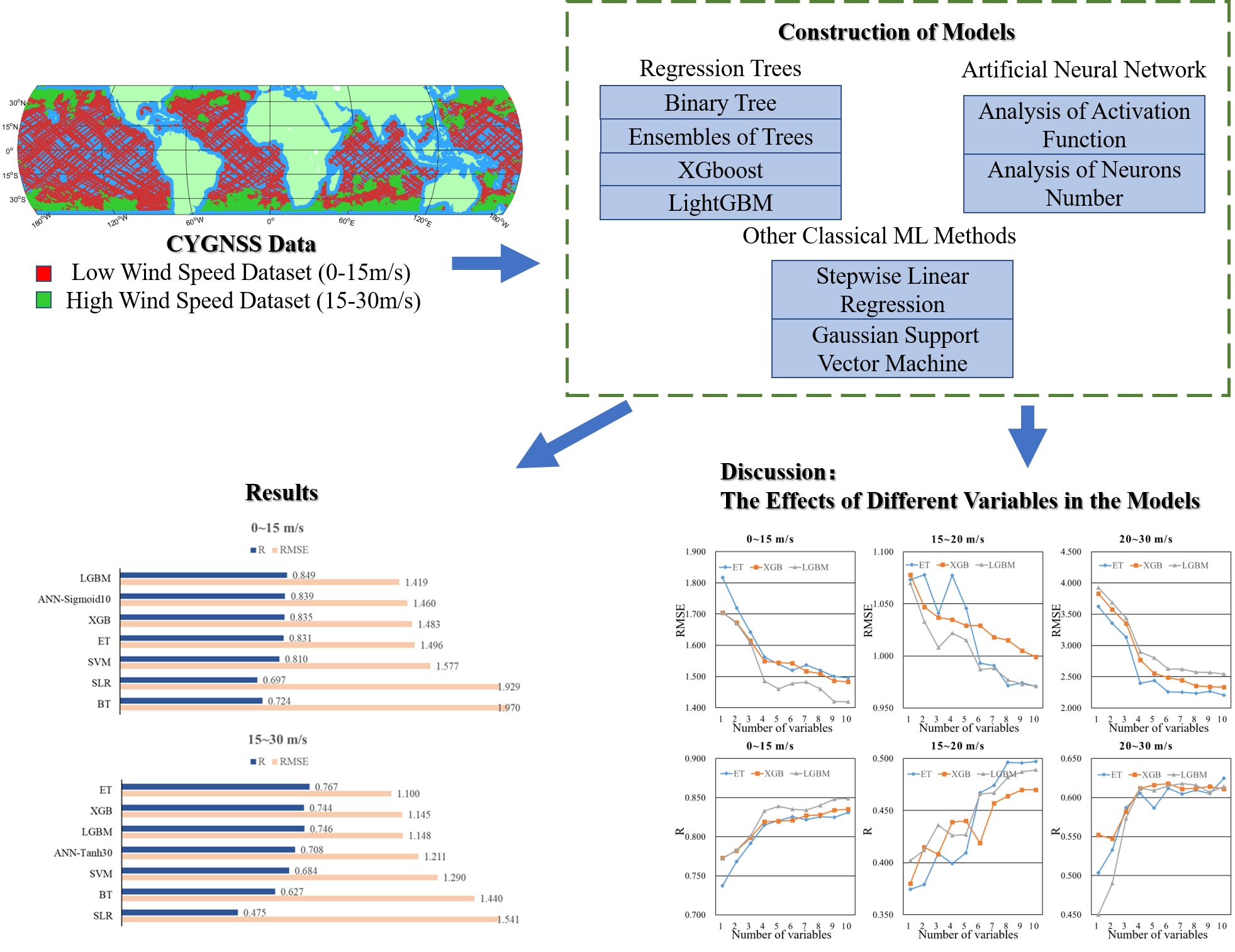
This paper focuses on sea surface wind speed estimation using L1B level v3.1 data of reflected GNSS signals from the Cyclone GNSS (CYGNSS) mission and European Centre for Medium-range Weather Forecast Reanalysis (ECMWF) wind speed data. Seven machine learning methods are applied for wind speed retrieval, i.e., Regression trees (Binary Tree (BT), Ensembles of Trees (ET), XGBoost (XGB), LightGBM (LGBM)), ANN (Artificial neural network), Stepwise Linear Regression (SLR), and Gaussian Support Vector Machine (GSVM), and a comparison of their performance is made. The wind speed is divided into two different ranges to study the suitability of the different algorithms. A total of 10 observation variables are considered as input parameters to study the importance of individual variables or combinations thereof. The results show that the LGBM model performs the best with an RMSE of 1.419 and a correlation coefficient of 0.849 in the low wind speed interval (0–15 m/s), while the ET model performs the best with an RMSE of 1.100 and a correlation coefficient of 0.767 in the high wind speed interval (15–30 m/s). The effects of the variables used in wind speed retrieval models are investigated using the XGBoost importance metric, showing that a number of variables play a very significant role in wind speed retrieval. It is expected that these results will provide a useful reference for the development of advanced wind speed retrieval algorithms in the future.

1. Introduction

With the continuous development of global navigation satellite systems (GNSSs), spaceborne GNSS reflectometry (GNSS-R) technology has become a hot research direction in the field of remote sensing. In 1993, Martín-Neira proposed the concept of the Passive Reflectometry and Interferometry System (PARIS) and the use of GNSS-R for ocean altimetry [1]. Since then, GNSS-R has been utilized for a range of ocean and land applications, including sea surface altimetry [2], sea surface wind speed measurements [3], sea ice detection [4], and soil moisture measurements [5]. Over the past few decades, a number of ground-based GNSS-R experiments have been conducted. Many airborne experiments have also been conducted to investigate this new remote sensing technology. Notwithstanding some technological challenges, satellite-based GNSS-R technology has the advantages of low cost and great coverage in some applications [6]. Currently, there are more than 14 satellites in operation carrying a GNSS-R payload.

UK-DMC (United Kingdom—Disaster Monitoring Constellation), the first satellite carrying a GNSS-R receiver, was launched on 27 September 2003; data from this system have been used to sense ocean roughness. UK TDS-1 (TechDemoSat-1), the second GNSS-R satellite, was launched on the 8 July 2014. On the 15 December 2016, NASA launched eight microsatellites to form the cyclone GNSS (CYGNSS) constellation with the initial objective of monitoring hurricane intensity [7,8]. Both TDS-1 and CYGNSS have generated a large amount of data which can be downloaded for scientific research [9]. On the 5 June 2019, the BuFeng-1 A/B twin satellites, developed by CASTC (China Aviation Smart Technology Co., Shenzhen, China), were launched from the Yellow Sea. One focus of the satellite mission is on the sensing of sea surface wind velocities, and especially typhoons, using GNSS-R [10].

Sea surface wind speed is an important and commonly used ocean geophysical parameter [11]. The stability of the wind field plays an important role in ocean circulation and global climate [12,13]. Traditional sea surface wind field monitoring methods generally use buoys or coastal meteorological stations, but these methods can only cover small areas with low spatial resolution and expensive equipment [14]. Microwave scatter meters and synthetic aperture radars can also monitor the global sea surface wind field [15,16]. Compared with these traditional wind measurement methods, spaceborne GNSS-R has several advantages, such as rich signal sources and all-weather, all-day, low cost, and large coverage [17,18].

GNSS-R technology is basically mature in retrieving sea surface wind speeds. Zavorotny and Voronovich proposed the scattering model theory in 2000 [19], which can simulate different waveforms of GNSS reflection signals, thus inverting sea surface wind speeds by delayed waveform matching methods [20]. Since then, observations extracted from DDMs (Delay Doppler Maps) have been widely used. DDM is the basic observation data of airborne and spaceborne GNSS-R receivers [21]. Some DDM observations, such as DDM average (DDMA), are directly related to sea surface roughness [21]. Other DDM observations can be used as variables for retrieving sea surface parameters. The normalized bistatic radar cross-section (NBRCS), leading edge slope (LES) and signal-to-noise ratio (SNR) have good correlations with the mean square slope (MSS) of the sea surface. Generally, the MSS is mainly affected by the sea surface wind speed [22].

In recent years, many spaceborne GNSS-R wind speed retrieval models have been developed. Jing et al. demonstrated the effectiveness of NBRCS by proposing some geophysical model functions (GMFs) related thereto [10]. Bu et al. proposed double- and triple-parameter GMFs with higher retrieval accuracy [14]. Machine learning methods have also been used to improve the performance of spaceborne GNSS-R wind speed retrieval. Liu Y. et al. proposed a machine learning algorithm based on a multi-hidden layer neural network. The accuracy of their models was significantly higher than that of GMFs [23]. Many subsequent studies have adopted similar algorithms and obtained results with RMSE of about 1.5–2.0 [24,25,26]. However, most of the above studies observed that it is difficult to use their algorithms to accurately retrieve high sea surface wind speeds [27,28]. A few studies have tried to enhance the ability of GNSS-R to retrieve high wind speeds. For instance, Zhang et al. developed machine learning-based models to retrieve wind speeds (20–30 m/s) with an RMSE of 2.64 and a correlation coefficient of 0.25 [29].

With high wind speed intervals, the Spaceborne GNSS-R data present different distributions and physical characteristics compared to when low wind speed intervals are applied, which leads to the inconsistent performance of different machine learning models. Therefore, this study analyzes the performance of various machine learning models in different wind speed intervals using the following methods: Regression trees (Binary Tree (BT), Ensembles of Trees (ET), XGBoost (XGB), LightGBM (LGBM) ), ANN (Artificial neural network), Stepwise Linear Regression (SLR), and Gaussian Support Vector Machine (GSVM). In this research, the selection of the input parameters for machine learning methods was significant. In this article, a range of variables are considered and evaluated, which are directly or indirectly relevant to sea surface wind speed. The main contributions of the article are as follows:

(1)

Seven machine learning methods are used to retrieve sea surface wind speed, and their performance is evaluated under two different wind speed ranges.

(2)

A ranking of the effects of 10 variables on wind speed retrieval is obtained by comparing the performance of different combinations of the variables. This provides a useful guide for variable selection when considering both complexity and accuracy.

(3)

A filtering algorithm is proposed to process DDM data, achieving both low complexity and good performance.

(4)

The effects of the number of neurons and activation functions on the performance of ANN wind speed retrieval are analyzed.

The rest of the paper is organized as follows. Section 2 introduces the GNSS-R variables and then describes the basic principles of the machine learning methods used in this study. Section 3 provides details of the applied data preprocessing strategies, the data filtering algorithm, and the construction of the machine learning-based model; the experimental results are also presented. Section 4 discusses the effects of the variables on wind speed retrieval. Section 5 presents the conclusions.

2. Methods

2.1. The CYGNSS Variables

2.1.1. Variables Calculated with DDM

The DDM glistening zone (the area from which scattered signals are observed) depends on the sea state, and the DDM volume has a significant correlation with wind speed [30,31]. Five variables (LES, DDMA, Noise Floor, SNR and NBRCS), extracted from DDM, can better reflect the sea state than the simple DDM volume [10,31]. Meanwhile, these variables are calibrated in the CYGNSS Level 1B product, which is commonly used for the retrieval of wind speed [32]. The LES of the integrated delay waveform, such as that generated with the delay waveforms of five different Doppler shifts, is strongly correlated with wind speed [33]. DDMA is the average of scattered power computed from the center 5 Doppler × 3 delay bin box [34], which is also significantly affected by wind speed. Noise Floor is the average power of DDM pixels which only contain noise. The signal-to-noise ratio (SNR) is defined as 10log(Smax/Noise Floor), where Smax is the maximum value in DDM, which has a strong correlation with sea surface roughness [35]. NBRCS is one of the two observables that were used to produce the global tropical cyclone product of CYGNSS [26], which is effective for wind speed retrieval [32].

2.1.2. Other Variables

In addition to the five variables derived from DDM data, five other variables were considered, representing the signal status, so that they can be used to enhance the performance of the models [8]. Instrument gain is the black body noise count divided by the sum of the black body power and the instrument noise power, which is an important parameter to calculate the DDM values. Scattering Area is the area of the central part of the DDM; generally, the larger this area, the rougher the reflective surface. Sp_inc_angle and sp_az_body are the incidence angle and azimuth angle of a given specular point, respectively. By taking sp_inc_angle and sp_az_body into account, the models can better reflect the situation of the received reflected signal [26]. Additionally, GNSS-R wind retrievals are affected by the ocean state [33]. Ocean swells are waves which travel from a long distance. The significant wave height of a swell (SWH_swell) will affect the reflection of the GNSS signals, which is a form of interference which can be used as a variable [27].

Table 1. List of input variables used in wind speed retrieval.

Input Variables	Long Name	Unit
NBRCS	Normalized bistatic radar cross-section	no unit
LES	Leading edge slope	no unit
SNR	DDM signal-to-noise ratio	dB
DDMA	DDM average	no unit
Noise Floor	DDM noise floor	no unit
sp_inc_angle	Specular point incidence angle	degree
sp_az_body	Specular point azimuth angle	degree
Instrument Gain	Instrument gain	no unit
Scatter Area	Scattering area of NBRCS and LES	square meter
SWH_swell	Significant wave height of ocean swell	meter

lists all the variables used in this study.

2.2. Regression Trees

Four out of the aforementioned seven machine learning algorithms comprise regression trees, which are briefly described in this subsection.

2.2.1. Binary Tree

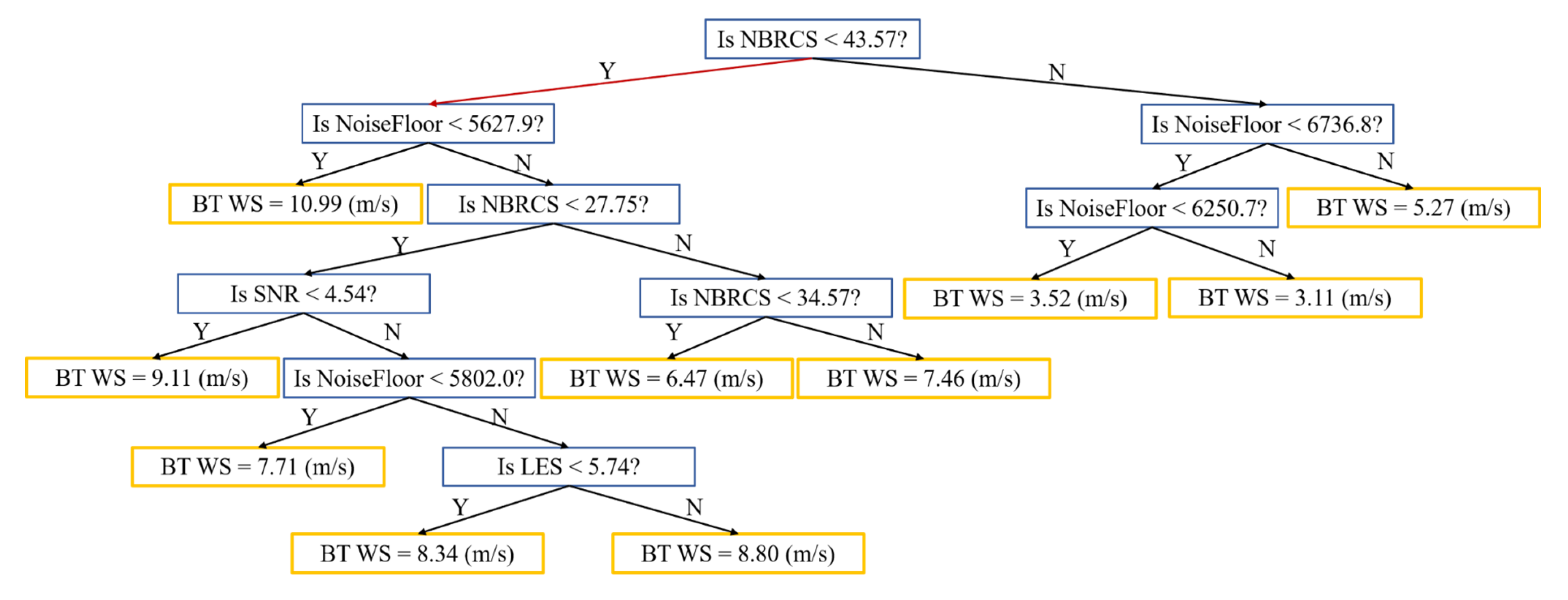
A binary tree (BT) is easy to interpret, fast for fitting and prediction, and low on memory usage. It consists of nodes and directed edges. There are two types of nodes: internal and leaf. In this paper, the internal nodes represent the variables of CYGNSS data and the leaf nodes represent the wind speed value. Each step in a prediction involves checking the value of one predictor variable. Figure 1 shows a simple sample BT composed of 100 CYGNSS-ERA5 matchups. In the experiments described in Section 3, the BT models are much more complex than this example, and the retrieval accuracy is much improved, because the amount of data used to build BT models is much larger.

When BT is used for regression tasks, variables of the sample are tested from the root node, and the sample is assigned to its child node according to the test results. In this way, the samples are tested and allocated recursively until they reach the leaf node, and each leaf node corresponds to a wind speed value. The criteria of splitting nodes are defined to balance predictive power and parsimony [36]. It is necessary to specify the minimum number of training samples used to calculate the response of each leaf node. When growing a regression tree, its simplicity and predictive power need to be considered at the same time. A very leafy tree tends to overfit, and its validation accuracy is often far lower than its training (or resubstitution) accuracy. In contrast, a coarse tree with fewer large leaves does not attain high training accuracy. However, a coarse tree can be more robust in that its training accuracy can be near that of a representative test set. In this paper, the minimum leaf size is set at 4.

2.2.2. Ensembles of Trees

Ensembles of Trees (ET) is one of the most popular techniques for building regression models [37,38]. Ensemble models combine results from many weak learners into one high-quality ensemble model. This approach has been applied frequently in fields such as remote sensing and statistics [39,40]. The function used to predict values is as follows:

$${\widehat{y}}_i={\displaystyle \sum }_{j=1}^K{f}_j\left(x_i\right), f_j\in F$$

(1)

where ${\widehat{y}}_i$ is the predicted value of the $i$-th sample, $K$ is the number of trees, $x_i$ is the $i$-th sample vector, $f_j$ denote the structure of the $j$-th independent tree and $F$ is the ensemble space of trees.

In this paper, a bagging tree is applied to build the ET. It draws its training set from the original sample set. In each round, n training samples are drawn from the original sample set using Bootstraping (some samples may be drawn multiple times in the training set, while some samples may not be drawn at all) [41]. A total of k rounds of extraction are performed to obtain k training sets, which means that k models will be built. The k training sets are independent of each other [42]. In this paper, k = 30 and the minimum leaf size is 8. Therefore, if several similar datasets are created by resampling with replacement and regression trees are grown without pruning, the variance component of the output error is reduced [41].

2.2.3. XGBoost

XGBoost (XGB) is a scalable, end-to-end tree boosting system which has been widely used in classification, regression and other machine learning tasks [43]. Based on Equation (1), XGBoost improves the running speed of model by using the regularized learning objective, which consists of two parts: the training loss term and regularization term, as given by:

$$Obj={\displaystyle \sum }_i^{N}l\left({\widehat{y}}_i,y_i\right)+{\displaystyle \sum }\mathsf{\Omega }\left(f_k\right)$$

(2)

where $l\left({\widehat{y}}_i,y_i\right)$ is the loss function which represents the deviation of ${\widehat{y}}_i$ (predicted value) from $y_i$ (true value); $\Omega \left(f_k\right)$ represents the complexity of the model as a regularization term, which helps to control the complexity of the model and avoid overfitting; and $N$ is the number of samples. In order to minimize the regularized learning objective as much as possible, Equation (2) will be minimized for multiple rounds. In each round, $f_t$ is added to Equation (2). The regularized learning objective of $t$-th round can be written as follows:

$$Ob{j}^{\left(t\right)}={\displaystyle \sum }_{i=1}^{N}l\left(y_i,{\widehat{y}}_i^{\left(t-1\right)}+f_t\left(x_i\right)\right)+\Omega \left(f_t\right)$$

(3)

The regularized learning objective can be approximated using the Taylor formula expansion:

$$Ob{j}^{\left(t\right)}\cong {\displaystyle \sum }_{i=1}^N\left(l\left(y_i,{\widehat{y}}_i^{\left(t-1\right)}\right)+g_i{f}_t\left(x_i\right)+\frac{1}{2}{h}_i{f}_t^2\left(x_i\right)\right)+\Omega \left(f_t\right)$$

(4)

where $g_i={\partial }_{{\widehat{y}}^{\left(t-1\right)}}l\left(y_i,{\widehat{y}}_i^{\left(t-1\right)}\right)$ is the first gradient statistics on the loss function, $h_i={\partial }_{{\widehat{y}}^{\left(t-1\right)}}^2 l\left(y_i,{\widehat{y}}_i^{\left(t-1\right)}\right)$ is the second gradient statistics on the loss function. The regularized learning objective of the $t$-th round is as follows:

$$Ob{j}^{\left(t\right)}={\displaystyle \sum }_{j=1}^T\left(G_j{w}_j+\frac{1}{2}(H_j+\lambda )w_j^2\right)+\gamma T$$

(5)

where $G_j={{\displaystyle \sum }}_{i\in I_j}{g}_i$ and $H_j={{\displaystyle \sum }}_{i\in I_j}{h}_i$ are the accumulation of $g_i$ and $h_i$, and $I_j$ denote the instance of $j$-th leaf. $T$ is the number of leaves in the tree. The optimal weight $w_j$ of the $j$-th leaf node can be determined as:

$$w_j=-\frac{G_j}{H_j+\lambda }$$

(6)

and the corresponding optimal value of the objective function $Ob{j}^{\left(t\right)}$ is given by:

$$Ob{j}^{\left(t\right)}=-\frac{1}{2}{\displaystyle \sum }_{j=1}^T\frac{G_j^2}{H_j+\lambda }+\gamma T$$

(7)

The parameter settings of XGBoost are shown in

Table 2. Parameter settings of XGBoost.

Parameter	Meaning	Value
n_estimators	Number of gradient boosted trees; equivalent to the number of boosting rounds.	100
importance_type	The type of variable importance	gain

.

2.2.4. LightGBM

LightGBM (LGBM) is an efficient gradient boosting decision tree, which serves to enhance the efficiency of the model when the variable dimension of the data sample is high and the data scale is large [44]. Compared with Xgboost, LightGBM is faster to compute and consumes less memory. LightGBM uses an Exclusive Feature Bundling (EFB) strategy to bundle mutually exclusive variables in order to reduce the number of variables and achieve the purpose of dimensionality reduction. Finding the optimal binding variable has been proven to be an NP-hard problem, as the enumeration method cannot be applied. In actual operation, EFB uses the greedy algorithm to approximate the optimal solution, i.e., which reduces the number of variables without affecting the accuracy of split nodes.

Table 3. Parameter settings of LightGBM.

Parameter	Meaning	Value
n_estimators	Number of boosted trees to fit	100
num_leaves	Maximum tree leaves for base learners	31
learning_rate	Boosting learning rate	0.1

shows the parameter settings of LightGBM.

2.3. Artificial Neural Network

Artificial neural networks (ANNs) are relatively new computational tools that have been used extensively to solve many complex real-world problems [45]. In order to avoid the effects of dimension and order of magnitude, before using an ANN to process data, the CYGNSS variables need to be normalized:

$$X_i^{\prime }=\frac{X_i-X_{min}}{X_{max}-X_{min}}$$

(8)

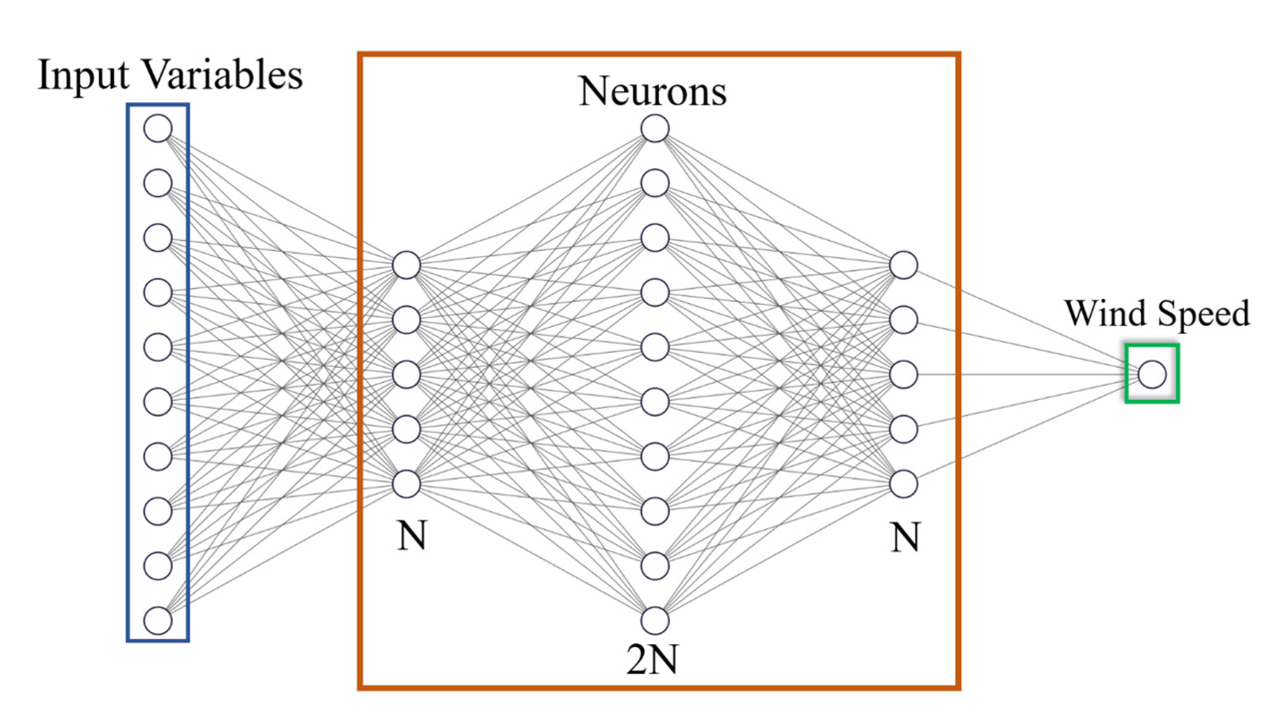
where $X_{min}$ and $X_{max}$ are the minimum and maximum values of the CYGNSS variables and $\left\{X_i^{\prime }\right\}$ are the normalized CYGNSS variables. The Full Connection Network (FCN) is often used in regression problems. Regarding GNSS-R wind speed retrieval, many researchers have demonstrated a significant improvement compared with traditional methods [23,25]. Figure 2 shows the ANN structure adopted in this paper, including input layers, hidden layers and the result of wind speed retrieval. Input layers are the 10 CYGNSS variables used in this paper. Three hidden layers are adopted; their neurons are N, 2N and N respectively. Figure 2 shows the structure of ANN when N = 5.

The number of neurons in an ANN affects the retrieval results, so the size of N is an important parameter when setting up a network. Herein, we analyze the impact of different activation functions on the performance of FCN, which makes connections between neurons. Generally, the accuracy of linear models is low, so activation functions improve the performance of ANN models by adding nonlinear factors. Determining the optimal activation function in an artificial neural network is an important task, because it is directly linked with the network performance. However, unfortunately, it is hard to determine this function analytically; rather, the optimal function is generally determined by trial and error or by tuning [46]. Three activation functions are analyzed in this paper, i.e., ReLu, Tanh and Sigmoid:

$$f_{ReLu}=\max \left(0,v\right)=\{\begin{array}{c}0 \left(v<0\right)\\ v \left(v\ge 0\right)\end{array}$$

(9)

$$f_{Tanh}=\frac{e^v-e^{-v}}{e^v+e^{-v}}$$

(10)

$$f_{Sigmoid}=\sigma \left(v\right)=\frac{1}{1+e^{-v}}$$

(11)

where $v$ is the input value of the previous neuron. The advantages of ReLU include the fast convergence speed of the network being trained, low computational complexity, and the absence of saturation and vanishing of gradient problems when $v$ > 0. The ReLU activation and combinations of multiple instances are non-linear. The Tanh function provides stronger non-linearity but is plagued from with saturating and vanishing gradient problems. The advantage of Tanh and Sigmoid is their stability.

2.4. Stepwise Linear Regression

Stepwise linear regression (SLR) is able to establish the optimal multi-variable linear regression equation. First, linear regression model $SL{R}^0$ is constructed with all variables $\left\{v_1,v_2,\dots ,v_p\right\}$:

$$f_{SLR}^0={\beta }_0+{\displaystyle \sum }_{i=1}^p{\beta }_i{v}_i$$

(12)

where $\left\{{\beta }_0,{\beta }_1,{\beta }_2,\dots ,{\beta }_p\right\}$ are constant parameters. The model is then used to estimate an unknown parameter such as wind speed for $n$ times, where $n$ is the number of observation datasets. The root mean square error (RMSE) of m estimations of model $SL{R}^0$ is calculated and denoted as $RMS{E}_0$. Next, the first variable, $v_1$, is removed, and estimation is performed m times again. Finally, the RMSE may be calculated and denoted as $RMS{E}_1$. If $RMS{E}_1$ is smaller than $RMS{E}_0$, $v_1$ may be removed; otherwise, it should be retained. This process is repeated until all variables are tested. Then, the variable with the smallest RMSE is selected. Therefore, this method is efficient for seeking localized variables [47]. SLR has good predictive ability and lower computational complexity than other methods [48].

2.5. Gaussian Support Vector Machine

Support Vector Machines (SVMs) are based on statistical learning theory, which contains polynomial classifiers, neural networks and radial basis function (RBF) networks in special cases. The SVM is thus not only theoretically well-founded but also superior in practical applications [49]. It is also commonly used to construct regression models. The function used to estimate the unknown parameter vector (such as the wind speed estimate vector) is given by:

$$f_{SVM}={\displaystyle \sum }_{i=1}^m{\displaystyle \sum }_{j=1}^m\left(l_i^{\prime }-l_i\right)\left(l_j^{\prime }-l_j\right)x_i^T{x}_j+b$$

(13)

where $m$ is the number of samples and $l_i^{\prime }$ and $l_i$ are the Lagrange multipliers. In this paper, $x$ is observation metric, which is composed of 10 variable rows and $m$ sample columns; $x_i$ and $x_j$ are the $i$-th column and $j$-th column, respectively; and $b$ is the threshold. By introducing the kernel functions replacing $x_i^T{x}_j$ with $K\left(x_i,x_j\right)$, where $K\left(x_i,x_j\right)$ is a transformation that maps $x_i$ to a high-dimensional space, the performance of the model can be improved. The choice of kernel function and parameters directly affects the performance of SVM [50]. The following are the commonly used positive semidefinite kernel functions, which are named as Linear function, Polynomial function and Gaussian function:

$$K\left(x_i,x_j\right)=x_i^T{x}_j$$

(14)

$$K\left(x_i,x_j\right)={\left(1+x_i^T{x}_j\right)}^p$$

(15)

$$K\left(x_i,x_j\right)=e^{-\Vert x_i-x_j{\Vert }^2}$$

(16)

After testing these kernel functions, it was found that the Gaussian function had the best effect in this study. Thus, Gaussian SVM (GSVM) is considered in this paper. In this study, the Box Constraint is 0.9762, the Epsilon is 0.09762 and the Kernel Scale is set at 3.7.

3. Experiments and Results

3.1. Data Processing Flow

This study makes use of the CYGNSS Level 1B (L1B) product, which contains Delay Doppler Maps (DDM), together with other engineering and science measurement parameters. CYGNSS data are in the range of 40°S to 40°N and work with a spatial resolution of ~25 km. The sampling rate of the data used in this study is 2 Hz. Different from most previous studies on wind speed estimation, this study adopts the latest CYGNSS v3.1 data instead of CYGNSS v2.1 data. Several data fields have been empirically corrected in the v2.1 L1 calibration algorithm. Therefore, they need to be carefully examined before modeling. Additionally, time-dependent variations have been observed in v2.1 data due to the variability of the transmitter and receiver. All these problems have been addressed in v3.1 data. The data are encapsulated by NASA in the netCDF file format and can be downloaded from https://podaac.jpl.nasa.gov/dataset/CYGNSS_L1_V3.1 (accessed on 26 March 2022) [29,30].

ECMWF reanalysis data (i.e. ERA-5) were used as the ground-truth data. ECMWF obtains hourly ERA-5 reanalysis datasets by assimilating meteorological data from different sources. The current sea surface wind speed product of ECMWF can be used as the ground-truth data in CYGNSS sea surface wind speed retrieval [25]. In this study, we use two ERA-5 parameters: the 10 m (above sea surface) u-component of neutral wind speed $W{S}_{u10}$ and the 10 m v-component of wind speed $W{S}_{v10}$, i.e., the eastward component and the northward component of the 10 m wind speed. The horizontal wind speed of 10 m above sea surface $W{S}_{10}$ can be readily obtained as the root square of the sum of the squares of these two parameters. However, CYGNSS data are sampled at an interval of half second and therefore need to be matched temporally with ERA-5 data. The spatial resolution of ERA-5 is 0.5° × 0.5°, which is rather different from that of CYGNSS, so spatial matching is also required.

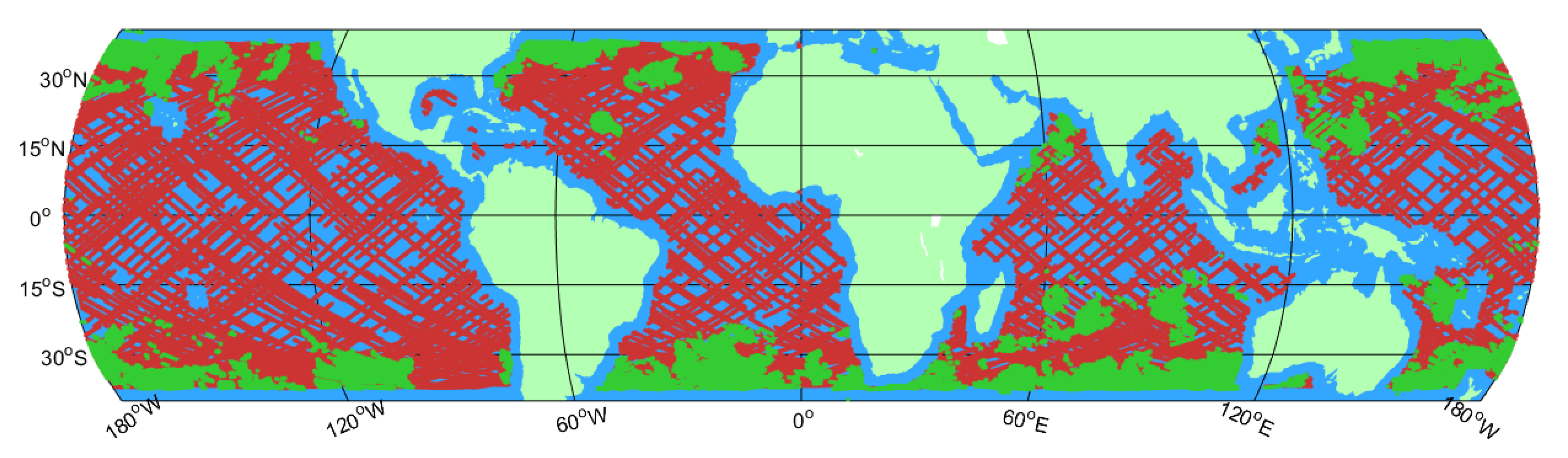
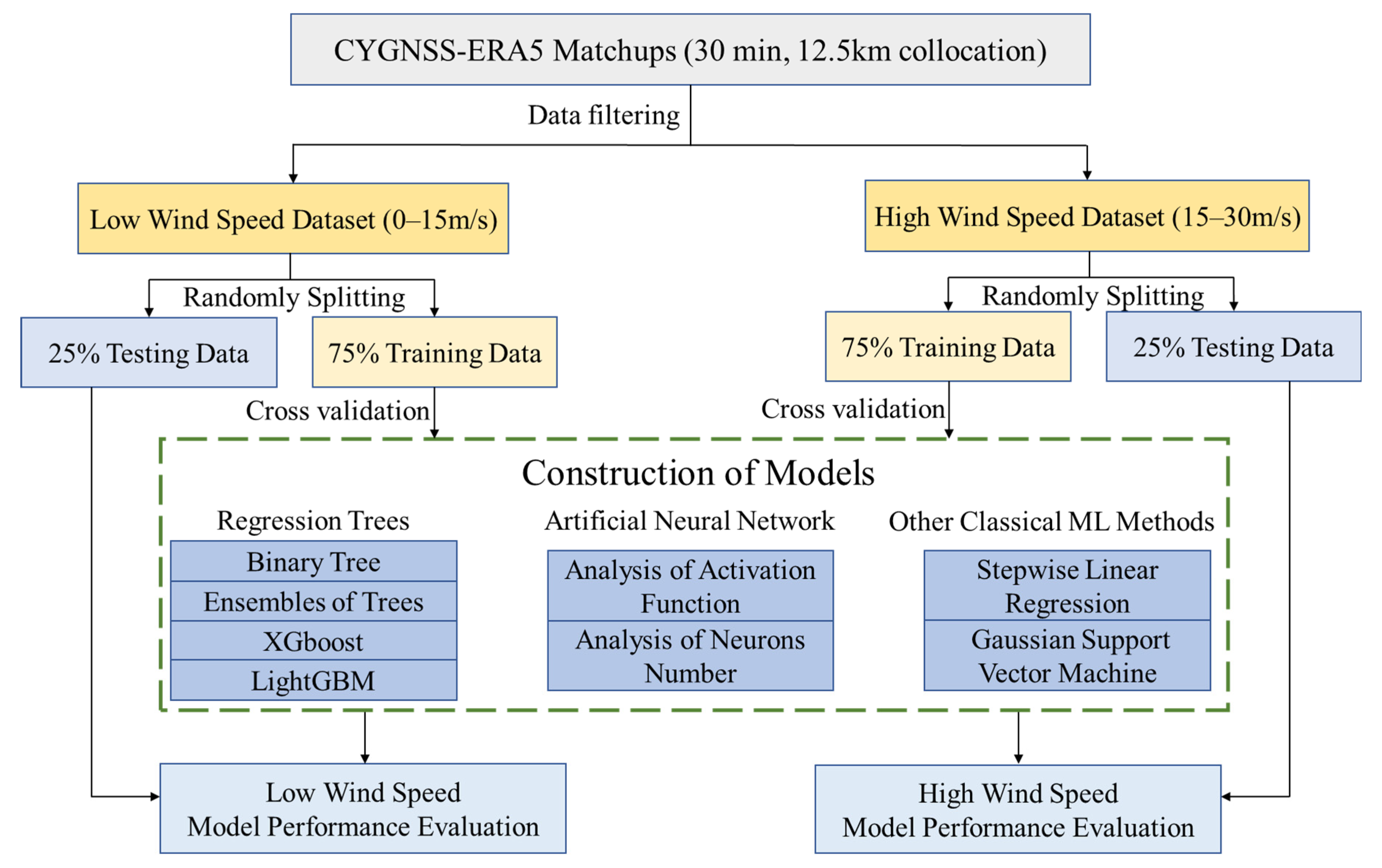
In order to analyze the performance of the machine learning methods in different wind speed intervals, two datasets are constructed according to the wind speed distribution. They are a low wind speed dataset with wind speeds within 0–15 m/s and a high wind speed dataset with wind speeds within 15–30 m/s. To ensure the data is representative and generalizable, and to improve the generalization ability of the models, this study mainly uses randomly selected data from 2019 to 2021. Figure 3 shows the spatial distribution of all data used in this paper. Red points represent low wind speed data and green points represent high wind speed data. Most high wind speed data generally appear in high latitudes, while low wind speed data appear in all latitudes. It should be noted that the sea surface roughness near the coast may be affected by land [6], which leads to performance degradation of GNSS-R technology in terms of retrieving sea surface wind speeds and other parameters [26].

The process of wind speed retrieval can be briefly summarized as containing four steps:

(1)

Selecting the datasets used in this study and dividing them into a training set and a testing set in a proportion of about 3:1;

(2)

Filtering the data;

(3)

Training the processed data with the machine learning methods described in Section 2. It should be noted that five folders cross validation is adopted when training the model. By dividing the dataset into several folders and estimating the accuracy of each fold, the cross validation prevents over fitting.

(4)

Evaluating the performance of different models by using test data.

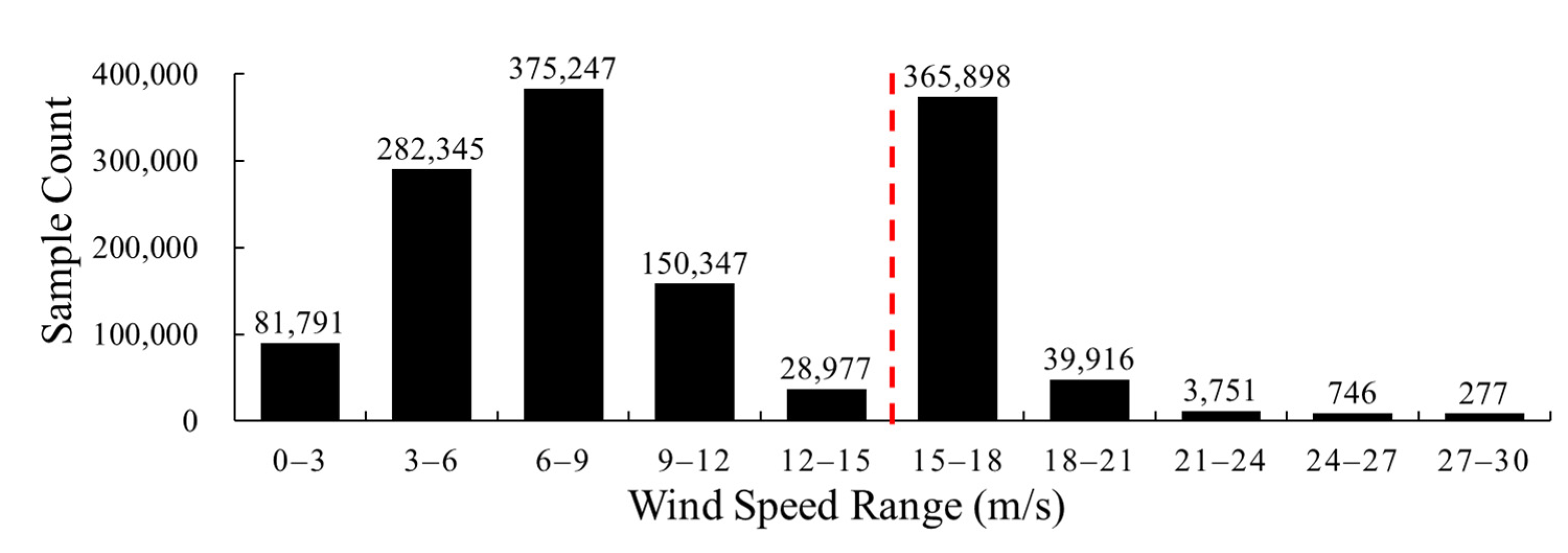
Figure 4 shows a flow chart of the proposed model construction and evaluation methods. Figure 5 shows the histogram of wind speed distribution. High wind speed data are more difficult to obtain than low wind speed data, and a great deal of the former are concentrated in the range of 15–20 m/s. Next, in order to evaluate the performance of the models and the effect of variables, three metrics are chosen, i.e., the root mean square error (RMSE), the correlation coefficient (R) and mean difference (MD), defined as:

$$RMSE=\sqrt{\frac{1}{n}{\displaystyle \sum }_{i=1}^n{\left(X_i-Y_i\right)}^2}$$

(17)

$$R=\frac{{{\displaystyle \sum }}_{i=1}^n\left(X_i-\overline{X}\right)\left(Y_i-\overline{Y}\right)}{\sqrt{{{\displaystyle \sum }}_{i=1}^n{\left(X_i-\overline{X}\right)}^2{{\displaystyle \sum }}_{i=1}^n{\left(Y_i-\overline{Y}\right)}^2}}$$

(18)

$$MD=\frac{1}{n}{\displaystyle \sum }_{i=1}^n\left(Y_i-X_i\right)$$

(19)

where n is the number of total data samples, {X_i} are the wind speed estimates, {Y_i} are the wind speed data of ERA5, $\overline{X}$ is the mean of {X_i} and $\overline{Y}$ is the mean of {Y_i}.

3.2. Data Filtering

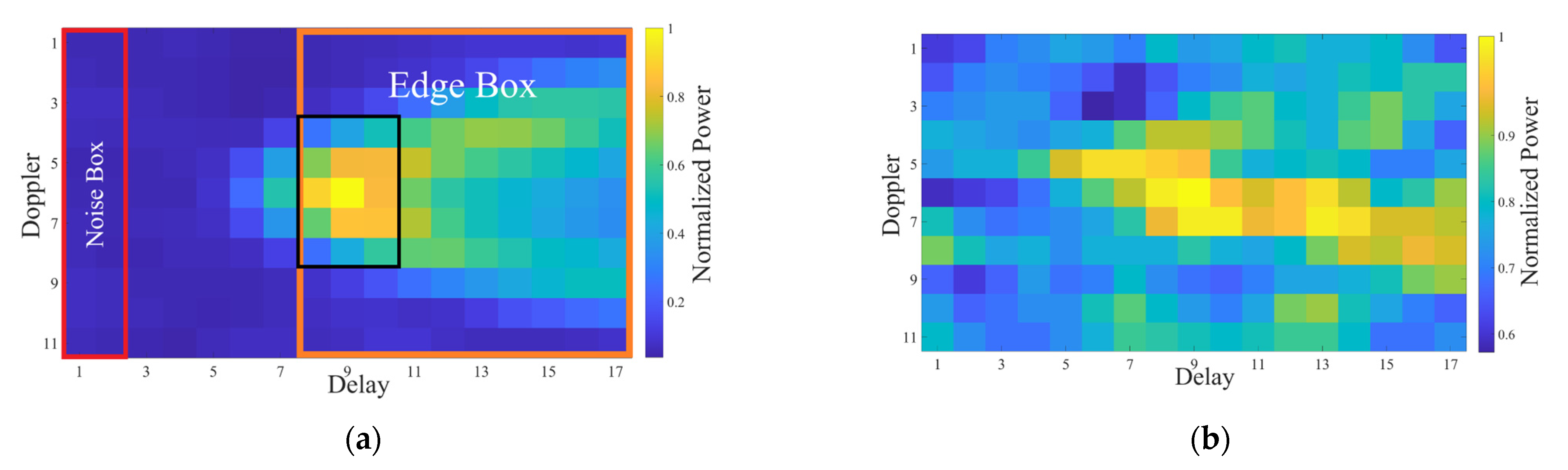
In this study, after discarding all abnormal values of observations (marked with NaN and negative numbers) and using quality control (QC) flags, a filtering algorithm based on DDM images is proposed. CYGNSS DDM is composed of 11 Doppler rows and 17 delay columns. When the signal condition is poor, the DDMs obtained by GYGNSS will not have an obvious horseshoe shape [14]. Such DDMs are unable to represent the MSS of the reflected surface effectively, and therefore, cannot be used for sea surface wind speed retrieval. In order to analyze the shapes of DDMs more easily, all DDMs are normalized according to:

$$nDDM\left(\tau ,f\right)=\frac{DDM\left(\tau ,f\right)}{DD{M}_{max}}$$

(20)

where $nDDM\left(\tau ,f\right)$ represents the measured power of the reflected signal when the time delay and frequency shift are $\tau$ and $f$ in the normalized DDM. $DD{M}_{max}$ represents the maximum power in the original DDM. CYGNSS compresses the DDM from a 128 × 20 matrix to a 17 × 11 matrix [6]. The red solid box in Figure 6a indicates the selected area of the noise floor part where the signal is absent. All the data whose noise floor maximum powers exceed the threshold value of 0.4 are excluded. This step screens out most of the DDMs influenced by noise without involving much computation. Some remaining DDMs may still be influenced by noise, so it is necessary to verify whether a basic horseshoe-shaped emerges. In order to reduce computation, this paper proposes a parameter called $EdgeA$, i.e., the difference between the mean value of the Edge Box and the mean of the noise floor. The orange and red boxes in Figure 6a indicate the trailing edge part and the floor noise part of the DDMs, respectively. The mean value of the noise floor is derived from Equation (21) [30], and $EdgeA$ is derived from Equation (22).

$$Nois{e}_{floor}=\frac{1}{N_1}{\displaystyle \sum }_{i=1}^2{\displaystyle \sum }_{j=1}^{11}nDDM\left({\tau }_i,f_j\right)$$

(21)

$$EdgeA=\frac{1}{N_2}{\displaystyle \sum }_{i={\tau }_{max}}^2{\displaystyle \sum }_{j=1}^{11}nDDM\left({\tau }_i,f_j\right)-Nois{e}_{floor}$$

(22)

where $N_1$ and $N_2$ are the number of all power values in the noise box and edge box. ${\tau }_{max}$ is the column number when the power of nDDM is maximum. In this study, $EdgeA$ must be greater than 0.1 to ensure that all DDMs have a basic horseshoe shape.

3.3. The Results of Regression Trees

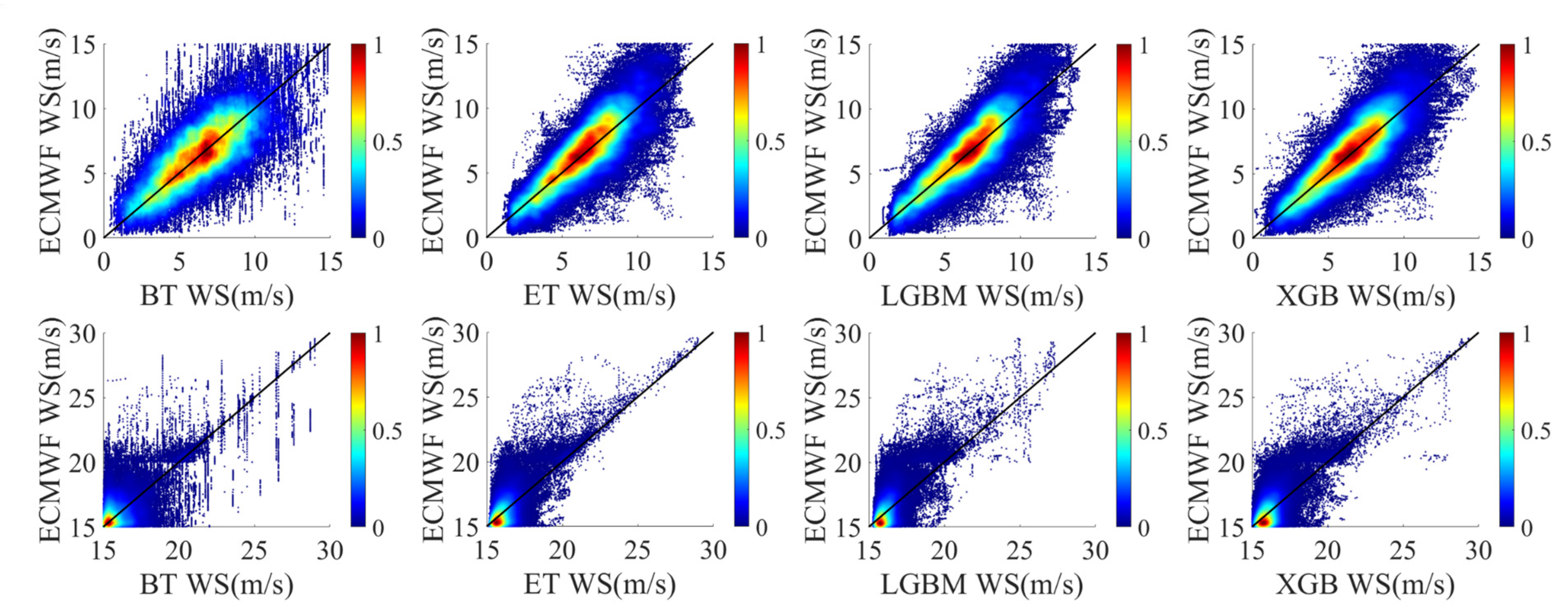
This section analyzes the effects of the four regression trees modeling methods (i.e., BT, ET, XGB and LGBM) that were described in Section 2.3. Figure 7 shows the scatter plots of the true and estimated wind speeds. In the figure, the color (from cool to warm) indicates the density of the points.

Table 4. The retrieval performance of each regression tree models.

Methods	0–15 (m/s)			15–30 (m/s)			15–20 (m/s)			20–30 (m/s)
	RMSE	R	MD	RMSE	R	MD	RMSE	R	MD	RMSE	R	MD
BT	1.970	0.724	0.089	1.440	0.627	0.150	1.320	0.300	0.070	2.577	0.567	1.255
ET	1.496	0.831	0.097	1.100	0.767	0.145	0.971	0.497	0.047	2.204	0.625	1.487
XGB	1.483	0.835	0.085	1.145	0.744	0.165	1.005	0.470	0.214	2.336	0.611	1.559
LGBM	1.419	0.849	0.066	1.148	0.746	0.162	0.971	0.489	0.210	2.542	0.614	1.961

shows the retrieval performance of each regression tree model. The bold font represents the best results. It may be seen that many high wind speed data are concentrated in the range of 15–20 m/s, causing elevated inversion accuracy in this range. In order to avoid the influence of data distribution on the analysis of the result, the performance of high wind speed models was analyzed in three data intervals: (1) overall (15–30 m/s), (2) 15–20 m/s and (3) 20–30 m/s.

As shown in Figure 7, all four regression tree-based modeling methods have the ability to retrieve wind speeds in different intervals. As the simplest regression tree modeling method, BT demonstrated the worst retrieval results, i.e., the greatest dispersion, as shown in Figure 7. Further analysis showed that the performance of the other three methods was superior to that of BT. LGBM had the best performance in the low wind speed interval; the RMSE and R of LGBM were improved by 27.97% and 17.27% compared with BT. In the high wind speed interval, the performance of ET was the best. For instance, the RMSE and R of ET were improved by 23.61% and 22.33% compared with BT. It should be noted that the RMSEs of high wind speed models are basically smaller than those of low wind speed models, which does not mean that the former have better performance in general. In fact, this situation is mainly affected by the wind speed distribution of the dataset used in this paper. The performance of all regression trees modeling methods was better in low wind speed interval, which is consistent with the conclusions of many previous studies [26,27,28,29]. From the calculated MD, a slight underestimation of true wind speed in both figures was observed. Besides, more obvious underestimations at high winds were shown by both models. This result is similar to that of [28]. Most of the research results demonstrate that GNSS-R data are more suitable for retrieving low wind speeds, while significant performance degradation occurs when retrieving high wind speeds [27,28,29]. This might be due to the reduced sensitivity of an ocean scattering cross-section to the high wind speed and the increased random error in the DDM signal [14].

3.4. The Results of ANNs

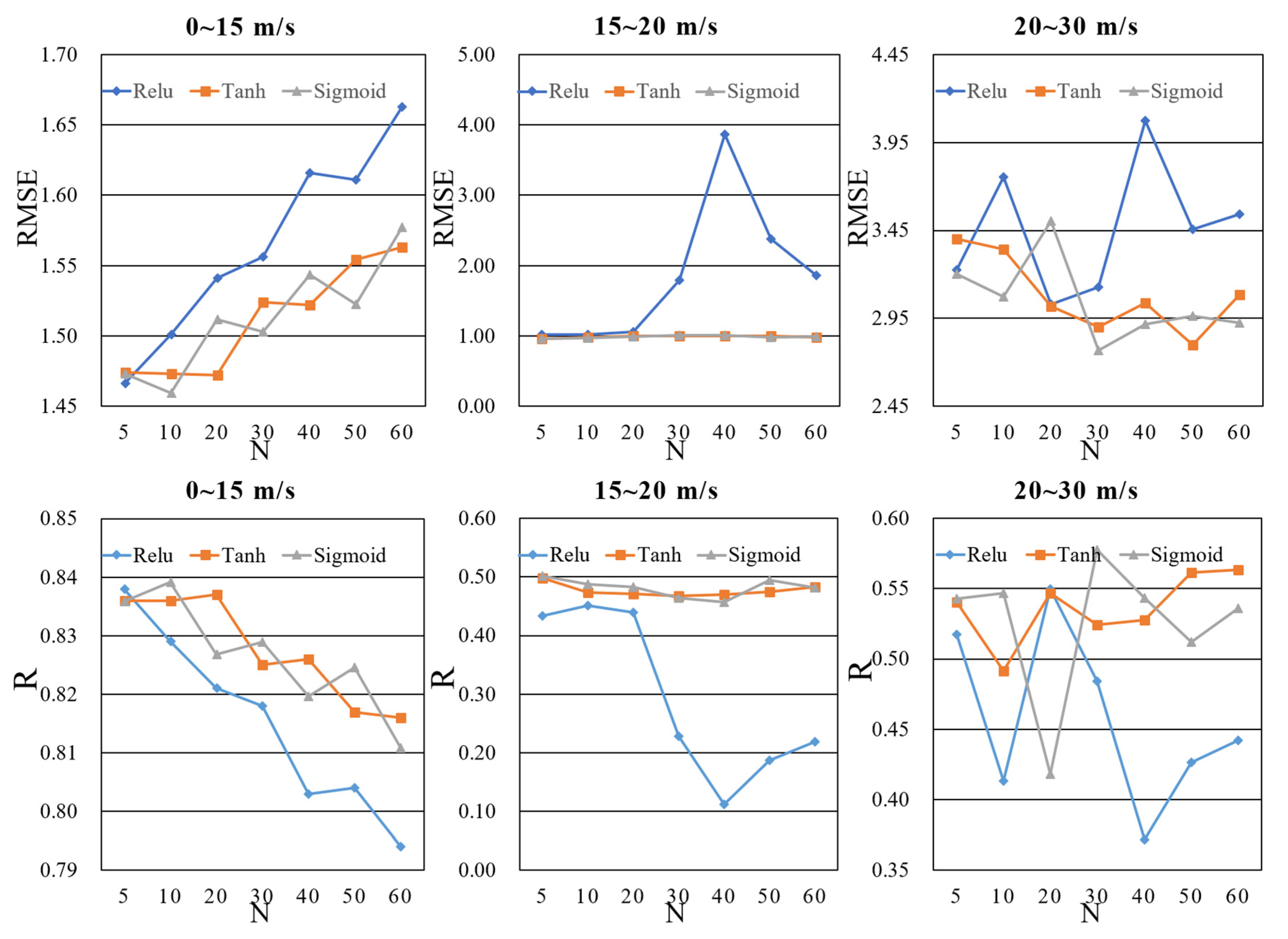
As shown in Figure 2, we adopted the three-layer neural network structure; the number distribution of three-layer neurons was N-2N-N. In this section, the influence of the value of N and activation function is analyzed. N is set at 5, 10, 20, 30, 40, 50 and 60, respectively.

Table 5. RMSEs of the ANN models.

N	0–15 (m/s)			15–30 (m/s)			15–20 (m/s)			20–30 (m/s)
	Relu	Tanh	Sigmoid	Relu	Tanh	Sigmoid	Relu	Tanh	Sigmoid	Relu	Tanh	Sigmoid
5	1.466	1.474	1.473	1.291	1.245	1.283	1.016	0.960	0.956	3.226	3.402	3.204
10	1.501	1.473	1.460	1.390	1.232	1.286	1.022	0.980	0.970	3.755	3.342	3.072
20	1.541	1.472	1.512	1.289	1.320	1.248	1.055	1.004	0.988	3.028	3.019	3.503
30	1.556	1.524	1.503	1.914	1.211	1.223	1.794	0.996	1.007	3.129	2.902	2.766
40	1.616	1.522	1.544	3.876	1.239	1.248	3.861	0.999	1.013	4.074	3.039	2.917
50	1.611	1.554	1.523	2.468	1.219	1.209	2.380	0.999	0.977	3.455	2.800	2.963
60	1.663	1.563	1.577	2.022	1.224	1.243	1.863	0.982	0.992	3.542	3.086	2.926

,

Table 6. Rs of the ANN models.

N	0–15 (m/s)			15–30 (m/s)			15–20 (m/s)			20–30 (m/s)
	Relu	Tanh	Sigmoid	Relu	Tanh	Sigmoid	Relu	Tanh	Sigmoid	Relu	Tanh	Sigmoid
5	0.838	0.836	0.836	0.659	0.695	0.671	0.434	0.498	0.501	0.518	0.540	0.543
10	0.829	0.836	0.839	0.635	0.699	0.665	0.452	0.473	0.487	0.413	0.491	0.547
20	0.821	0.837	0.827	0.662	0.667	0.685	0.440	0.471	0.482	0.550	0.547	0.418
30	0.818	0.825	0.829	0.453	0.708	0.703	0.228	0.468	0.464	0.484	0.524	0.578
40	0.803	0.826	0.820	0.264	0.693	0.687	0.112	0.470	0.457	0.372	0.527	0.543
50	0.804	0.817	0.825	0.385	0.703	0.708	0.187	0.475	0.495	0.426	0.562	0.512
60	0.794	0.816	0.811	0.455	0.702	0.690	0.219	0.483	0.481	0.442	0.563	0.536

and

Table 7. MDs of the ANN models.

N	0–15 (m/s)			15–30 (m/s)			15–20 (m/s)			20–30 (m/s)
	Relu	Tanh	Sigmoid	Relu	Tanh	Sigmoid	Relu	Tanh	Sigmoid	Relu	Tanh	Sigmoid
5	0.047	0.038	0.036	0.192	0.183	0.208	0.022	0.005	0.017	2.533	2.633	2.833
10	0.050	0.028	0.027	0.117	0.183	0.192	0.016	0.021	0.009	1.509	2.423	2.703
20	0.062	0.040	0.053	0.160	0.137	0.152	0.009	0.045	0.007	2.233	1.400	2.148
30	0.071	0.028	0.050	0.172	0.100	0.182	0.036	0.011	0.061	2.043	1.321	1.849
40	0.084	0.080	0.087	0.165	0.191	0.175	0.040	0.046	0.037	1.877	2.198	2.075
50	0.077	0.064	0.083	0.122	0.165	0.144	0.012	0.017	0.021	1.630	2.194	1.843
60	0.056	0.064	0.095	0.113	0.136	0.184	0.004	0.022	0.029	1.619	1.688	2.315

show the RMSEs, Rs and MDs of the wind speed retrieval using ANN models with different activation functions and N values, respectively. As in Section 3.3, the bold font represents the best result, and the performance of the high wind speed models was analyzed in three data intervals. Figure 8 shows RMSEs and Rs of the wind speed retrieval models in a more intuitive form, i.e., in the form of line chart.

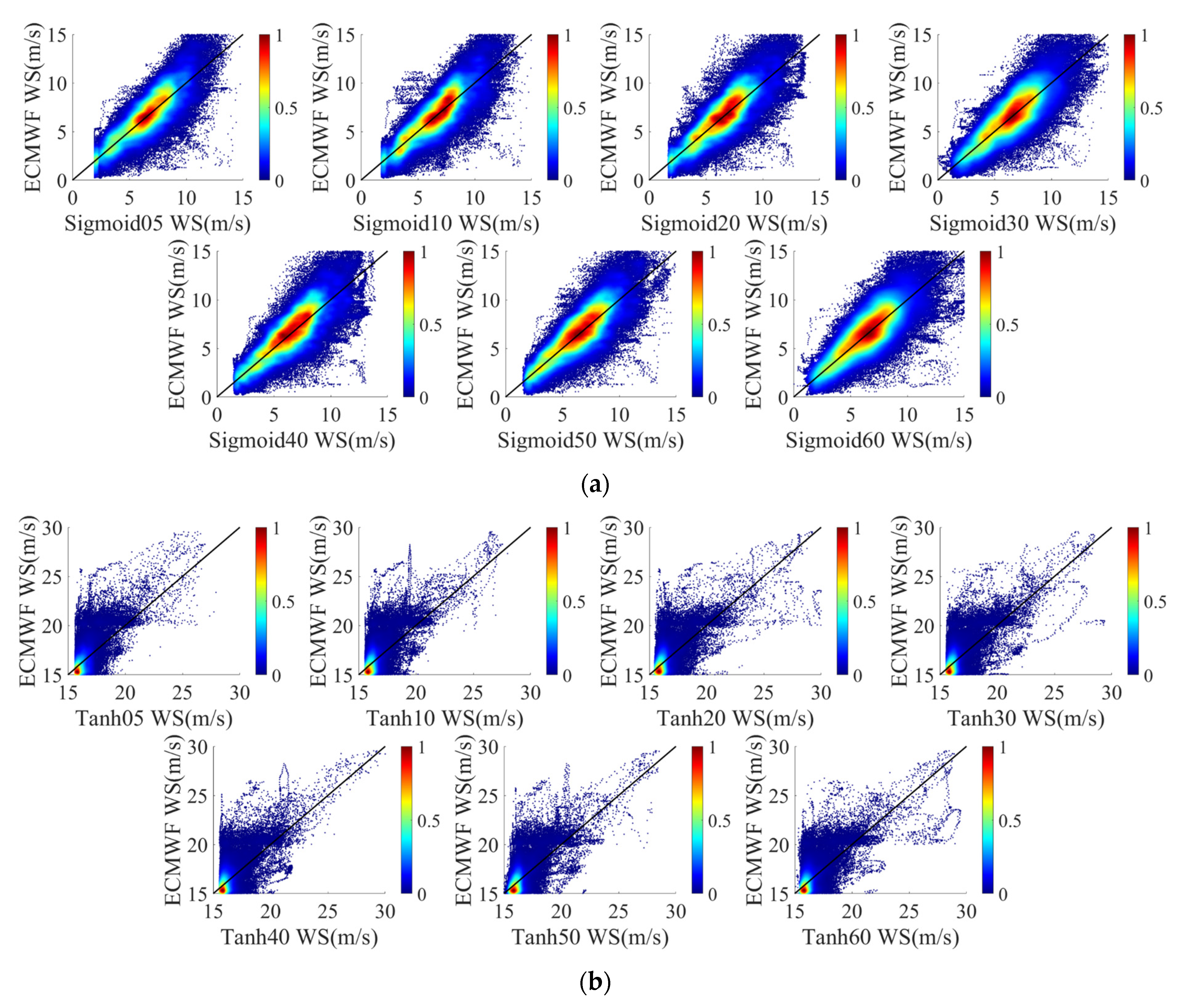
In the low wind speed interval, it is obvious that the choice of activation function hardly affected the ANN models, as shown in Figure 8. However, the increase of the number of neurons significantly reduced the accuracy of the models, although the accuracy variation was not very significant. In the high wind speed interval, the increase in the number of neurons had little effect on Sigmoid and Tanh, but it had an obvious effect on ReLu. As shown in Table 6, for a low wind speed interval, when the activation function was Sigmoid and N was 10, the performance of ANN was the best. For a high wind speed interval, when the activation function was Tanh and N was 30, the performance of ANN was the best. Overall, although the underestimation of ANNs at high winds was smaller than that of regression trees, the retrieval performance of ANNs was slightly worse than that of the regression tree modeling methods. In order to facilitate a comparison with other methods, scatter plots of low wind speeds retrieved by the Sigmoid function and of high wind speeds retrieved by the Tanh function are presented as examples, as shown in Figure 9.

3.5. The Results of SLR and SVM

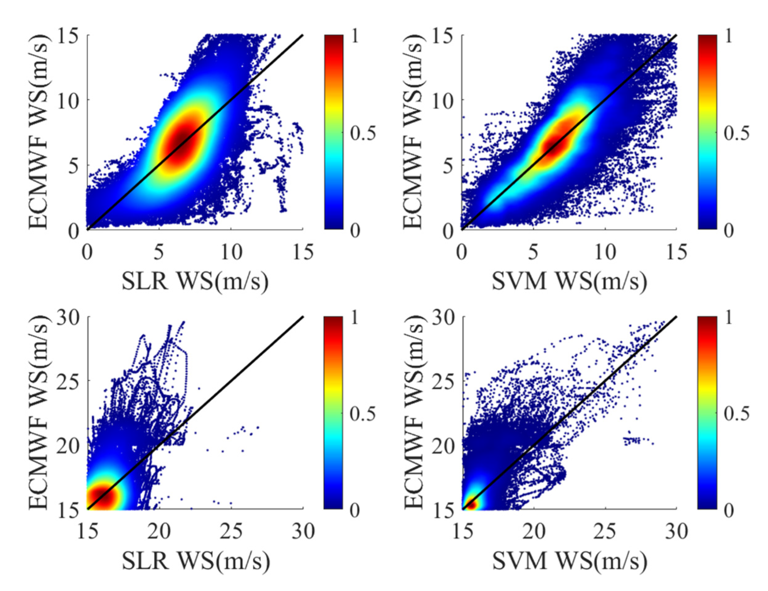
This section analyzes the effects of two other classical machine learning methods (i.e., SLR and SVM), as described in Section 2.4 and Section 2.5. Figure 10 shows scatter plots of the true and estimated wind speeds.

Table 8. Retrieval performance of SLR and SVM.

Methods	0–15 (m/s)			15–30 (m/s)			15–20 (m/s)			20–30 (m/s)
	RMSE	R	MD	RMSE	R	MD	RMSE	R	MD	RMSE	R	MD
SLR	1.929	0.697	0.055	1.541	0.475	0.364	1.213	0.280	0.199	3.844	0.393	3.456
SVM	1.577	0.810	−0.021	1.290	0.684	0.304	1.007	0.488	0.075	3.254	0.556	2.623

shows the retrieval performance of each regression trees model. Similarly, the bold font represents the best result, and the performance of high wind speed models was analyzed in three data intervals. It is obvious that the retrieval results of SVM had less dispersion than those of SLR, which means that the performance of SVM was better. However, the retrieval performance of the models described in the previous two sections was better than that of the models presented in this section.

3.6. Summary

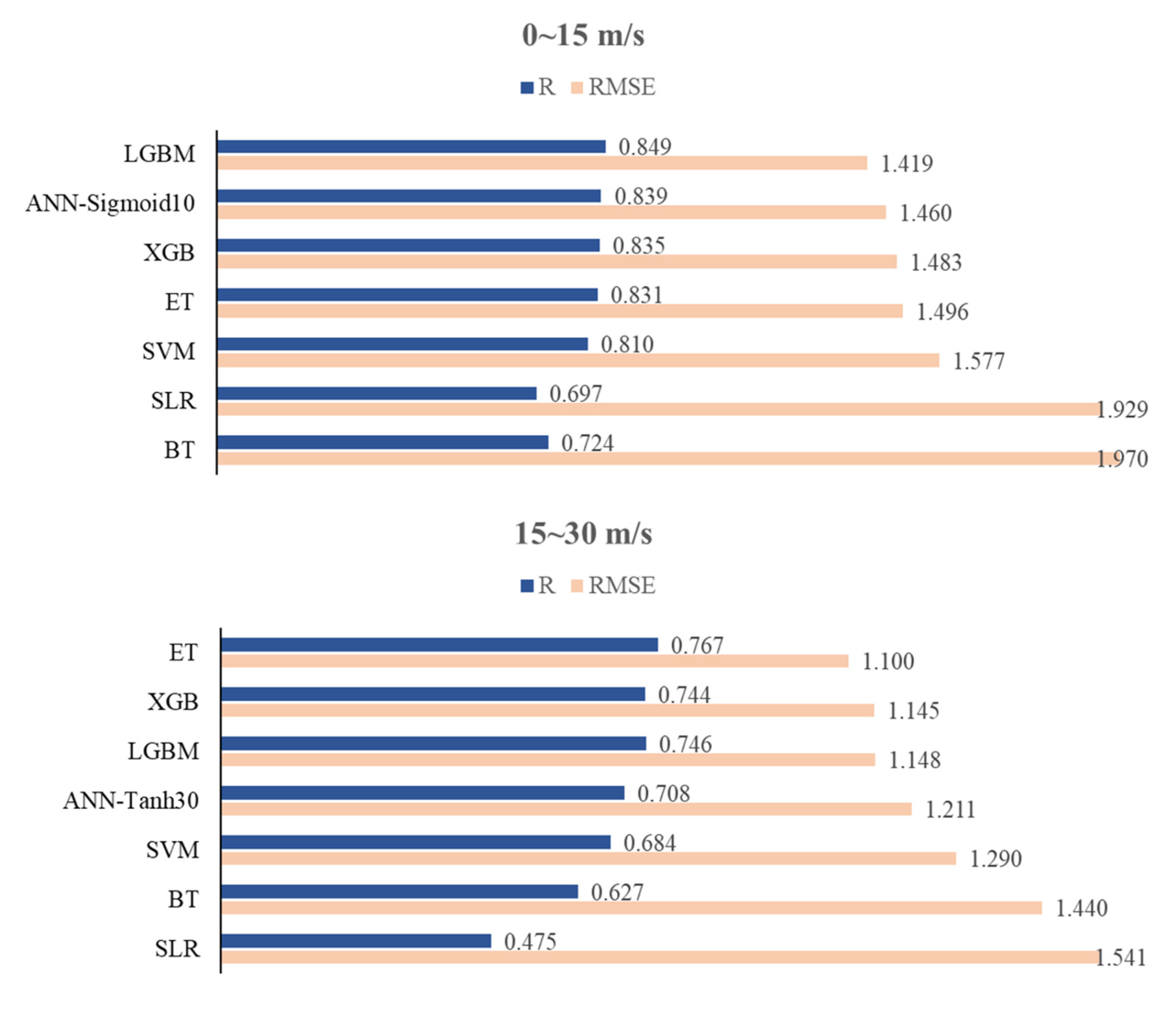
The preceding subsections presented and analyzed the retrieval performance of several machine learning methods in different wind speed intervals. This subsection summarizes and analyzes their performance gaps. Figure 11 shows the Rs and RMSEs of the models using machine learning methods. It is obvious from Figure 11 that the RMSE of LGBM is smaller than those of other models in a low wind speed interval, while the RMSE of ET is smaller than those of other models in a high wind speed interval. The R values are usually larger when the RMSE values are smaller. The performance of LGBM, ET, ANN and XGB are significantly better than that of SVM, BT and SLR, which means that they are more suitable for wind speed retrieval.

4. Discussion

By analyzing the performance of all seven models, it can be concluded that LGBM performed best in the low wind speed interval, while ET performed best in the high wind speed interval. However, the above experimental results do not prove that all the variables in Table 1 can be used to optimize the performance of the model. On the contrary, some variables may reduce the accuracy of the model. Therefore, it is very important to analyze the effects of different variables. It should be noted that in the high wind speed interval, the data of spaceborne GNSS-R also present different data distributions and characteristics from those in the low wind speed interval, and the roles of the variables were not always consistent. Here, we use the characteristics of XGBoost as the basis for evaluating the effect of each variable. XGBoost uses the average gain (AG) of data splits across all trees to measure the effects of variables [51]. After model training, by analyzing the XGBoost model structure, the AG related to each variable is defined as:

$$A{G}_{v_i}=\frac{{\displaystyle \sum }Gai{n}_{v_i}}{S_{v_i}}$$

(23)

where $v_i$ is a variable used in the XGBoost model, $S_{v_i}$ is the number of times that $v_i$ is used to split the data across all trees and $Gai{n}_{v_i}$ is the gain value of each tree after splitting with $v_i$.

Table 9. Rankings of the effects of variables.

0–15 (m/s)			15–30 (m/s)
Rank	AG	Variables	Rank	AG	Variables
1	9452.12	NBRCS	1	364.99	SWH_swell
2	2649.02	LES	2	100.85	NoiseFloor
3	1887.14	SNR	3	90.88	NBRCS
4	1602.55	SWH_swell	4	88.56	ScatterArea
5	443.67	InstGain	5	84.76	InstGain
6	360.00	NoiseFloor	6	76.91	AzBody
7	337.60	DDMA15	7	73.86	DDMA15
8	320.35	ScatterArea	8	71.09	IncAngle
9	284.02	AzBody	9	64.71	SNR
10	253.56	IncAngle	10	44.97	LES

shows the AG of each variable in the low and high wind speed intervals, respectively.

Although AG helps to verify the effectiveness of feature selection, it cannot be used as a direct basis thereof. As such, the rationale of Table 9 needs to be demonstrated through experimental results. In order to analyze the influences of different variables more intuitively, this study constructed 60 models based on ET, XGB and LGBM with different variables. Line charts were used to help in analyzing the influence of these variables. The x-axis in Figure 12 indicates the number of variables, which is consistent with the ranking of the effects of variables in Table 9. For example, in the low wind speed interval, if the number of variables was set at 4, NBRCS, LES, SNR and SWH_swell were used in the modeling; in the high wind speed interval, if the number of variables was set at 3, SWH_swell, NoiseFloor and NBRCS were used in the modeling.

In Figure 12, the relationship between variables and models can be analyzed clearly. It is obvious that Figure 12 and Table 9 are highly consistent. In the low wind speed interval, the AG of NBRCS is much larger than that of other variables, which means that NBRCS is the most important variable in the low wind speed models. In the two subgraphs of the first column of Figure 12, it is obvious that LES, SNR and SWH_swell improved the performance of the model greatly, as also confirmed in Table 9. In Table 9, the AGs of LES, SNR and SWH_swell are significantly greater than those of the other variables. These variables effectively reduced the RMSE of the model and increased the correlation coefficient between the wind speed estimates and the true values of wind speed. In the high wind speed interval, the models were mostly affected by SWH_swell; this may have been due to the degradation of the performance of spaceborne GNSS-R technology in a high wind speed. This result also indicates that, especially in the high wind speed interval, spaceborne GNSS-R technology needs to fuse more reliable auxiliary information to achieve better retrieval results. The contributions of other variables to the model are basically similar. Different from the results of the low wind speed interval, the effects of NoiseFloor and ScatterArea were significantly greater, while the effects of SNR and LES were lower. In the high wind speed interval, the quality of DDM became lower, decreasing the correlation coefficients between sea surface MSS and the variables SNR and LES.

In general, from the above analysis, it is obvious that the results of the models with all variables are the best in both high and low wind speed intervals. In most cases, the accuracy of the model is directly proportional to the number of variables. Additionally, for different modeling methods, the influence of the number of variables was different; for different wind speed intervals, the rankings of the effects of variables were different. The above conclusions may be helpful for the future research of spaceborne GNSS-R sea surface wind speed retrieval.

5. Conclusions

By using machine learning methods, this study investigated wind speed retrieval in different wind speed intervals. Through extensive processing of experimental data, it was observed that different machine learning methods have different properties in different wind speed intervals. In particular, a range of multi-variable models was developed and evaluated. The results showed that the LGBM model performs best with an RMSE of 1.419 m/s and a correlation coefficient of 0.849 in the low wind speed interval (0–15 m/s), while the ET model performs best with an RMSE of 1.100 and a correlation coefficient of 0.767 in the high wind speed interval (15–30 m/s). In addition, through experiments, some characteristics of ANN models were found in wind speed retrieval. In the low wind speed interval, the choice of activation function hardly affects the ANN models, while the increase of the number of neurons significantly reduces the accuracy of the model. In the high wind speed interval, the increase in the number of neurons has little effect on Sigmoid and Tanh, but it has an obvious effect on ReLu.

The effects of the variables used in the wind speed retrieval models described in this paper were analyzed. Through processing experimental data, it was observed that the models with all variables (i.e. NBRCS, LES, SNR, DDMA, Noise Floor, sp_inc_angle, sp_az_body, Instrument Gain, Scatter Area, and SWH_swell) achieved the highest accuracy. In the low wind speed interval, NBRCS, LES, SNR and SWH_swell were the most important variables. In the high wind speed interval, the models were mostly affected by SWH_swell, and the ranking of the effects of variables was very different from that in the low wind speed interval.

Future studies will focus on further performance enhancements of the models developed in this paper. For instance, the accuracy of the model would decrease in the presence of large wind speed and high SWH_swell. It would thus be useful to develop techniques to handle the retrieval of high wind speeds with minimal performance degradation.

References

- Martin-Neira, M. A Passive Reflectometry and Interferometry System (PARIS): Application to ocean altimetry. ESA J. 1993, 17, 331–355. [Google Scholar]
- Hu, C.J.; Benson, C.R.; Qiao, L.; Rizos, C. The validation of the weight function in the leading-edge-derivative path delay estimator for space-based GNSS-R altimetry. IEEE Trans. Geosci. Remote Sens. 2020, 58, 6243–6254. [Google Scholar] [CrossRef]
- Clarizia, M.P.; Ruf, C.S. Wind speed retrieval algorithm for the Cyclone Global Navigation Satellite System (CYGNSS) mission. IEEE Trans. Geosci. Remote Sens. 2016, 54, 4419–4432. [Google Scholar] [CrossRef]
- Alonso-Arroyo, A.; Zavorotny, V.U.; Camps, A. Sea ice detection using UK TDS-1 GNSS-R data. IEEE Trans. Geosci. Remote Sens. 2017, 55, 4989–5001. [Google Scholar] [CrossRef] [Green Version]
- Arroyo, A.A.; Camps, A.; Aguasca, A.; Forte, G.F.; Monerris, A.; Rudiger, C.; Walker, J.P.; Park, H.; Pascual, D.; Onrubia, R. Dual-polarization GNSS-R interference pattern technique for soil moisture mapping. IEEE J. Sel. Top. Appl. Earth Obs. Remote Sens. 2014, 7, 1533–1544. [Google Scholar] [CrossRef]
- Peng, Q.; Jin, S.G. Significant wave height estimation from space-borne cyclone-GNSS reflectometry. Remote Sens. 2019, 11, 584. [Google Scholar] [CrossRef] [Green Version]
- Ruf, C.; Lyons, A.; Unwin, M.; Dickinson, J.; Rose, R.; Rose, D.; Vincent, M. CYGNSS: Enabling the future of hurricane prediction. IEEE Geosci. Remote Sens. Mag. 2013, 1, 52–67. [Google Scholar] [CrossRef]
- Gleason, S. CYGNSS Algorithm Theoretical Basis Documents, Level 1A and 1B; University of Michigan: Ann Arbor, MI, USA, 2018; pp. 4–19. [Google Scholar]
- Yu, K. Theory and Practice of GNSS Reflectometry; Springer Nature: Berlin/Heidelberg, Germany, 2021; pp. 1–376. [Google Scholar] [CrossRef]
- Jing, C.; Niu, X.L.; Duan, C.D.; Lu, F.; Di, G.D.; Yang, X.F. Sea surface wind speed retrieval from the first Chinese GNSS-R mission: Technique and preliminary results. Remote Sens. 2019, 11, 3013. [Google Scholar] [CrossRef] [Green Version]
- Huang, B.Y.; Stone, P.H.; Sokolov, A.P.; Kamenkovich, I.V. Ocean heat uptake in transient climate change: Mechanisms and uncertainty due to subgrid-scale eddy mixing. J. Clim. 2003, 16, 3344–3356. [Google Scholar] [CrossRef] [Green Version]
- Barthelmie, R.J. The effects of atmospheric stability on coastal wind climates. Meteorol. Appl. 1999, 6, 39–47. [Google Scholar] [CrossRef]
- Kirincich, A. Remote sensing of the surface wind field over the coastal ocean via direct calibration of HF radar backscatter power. J. Atmos. Oceanic Technol. 2016, 33, 1377–1392. [Google Scholar] [CrossRef]
- Bu, J.W.; Yu, K.G.; Zhu, Y.C.; Qian, N.J.; Chang, J. Developing and testing models for sea surface wind speed estimation with GNSS-R delay doppler maps and delay waveforms. Remote Sens. 2020, 12, 3760. [Google Scholar] [CrossRef]
- Jacobson, M.D.; Emery, W.J.; Westwater, E.R. Oceanic wind vector determination using a dual-frequency microwave airborne radiometer theory and experiment. In Proceedings of the IGARSS’96 1996 International Geoscience and Remote Sensing Symposium, Lincoln, NE, USA, 31 May 1996; pp. 1138–1140. [Google Scholar]
- Monaldo, F.M.; Thompson, D.R.; Beal, R.C.; Pichel, W.G.; Clemente-Colon, P. Comparison of SAR-derived wind speed with model predictions and ocean buoy measurements. IEEE Trans. Geosci. Remote Sens. 2001, 39, 2587–2600. [Google Scholar] [CrossRef]
- Liu, X.X.; Bai, W.H.; Xia, J.M.; Huang, F.X.; Yin, C.; Sun, Y.Q.; Du, Q.F.; Meng, X.G.; Liu, C.L.; Hu, P.; et al. FA-RDN: A hybrid neural network on GNSS-R sea surface wind speed retrieval. Remote Sens. 2021, 13, 4820. [Google Scholar] [CrossRef]
- Bu, J.W.; Yu, K.G. Sea surface rainfall detection and intensity retrieval based on GNSS-reflectometry data from the CYGNSS mission. IEEE Trans. Geosci. Remote Sens. 2022, 60, 1–15. [Google Scholar] [CrossRef]
- Zavorotny, V.U.; Voronovich, A.G. Scattering of GPS signals from the ocean with wind remote sensing application. IEEE Trans. Geosci. Remote Sens. 2000, 38, 951–964. [Google Scholar] [CrossRef] [Green Version]
- Komjathy, A.; Zavorotny, V.U.; Axelrad, P.; Born, G.H.; Garrison, J.L. GPS Signal scattering from sea surface: Wind speed retrieval using experimental data and theoretical model. Remote Sens. Environ. 2000, 73, 162–174. [Google Scholar] [CrossRef]
- Clarizia, M.P.; Ruf, C.S.; Jales, P.; Gommenginger, C. Spaceborne GNSS-R minimum variance wind speed estimator. IEEE Trans. Geosci. Remote Sens. 2014, 52, 6829–6843. [Google Scholar] [CrossRef]
- Ruffini, G.; Soulat, F.; Caparrini, M.; Germain, O.; Martin-Neira, M. The Eddy Experiment: Accurate GNSS-R ocean altimetry from low altitude aircraft. Geophys. Res. Lett. 2004, 31, 1–4. [Google Scholar] [CrossRef] [Green Version]
- Liu, Y.X.; Collett, I.; Morton, Y.J. Application of neural network to GNSS-R wind speed retrieval. IEEE Trans. Geosci. Remote Sens. 2019, 57, 9756–9766. [Google Scholar] [CrossRef]
- Asgarimehr, M.; Wickert, J.; Reich, S. Evaluating impact of rain attenuation on space-borne GNSS reflectometry wind speeds. Remote Sens. 2019, 11, 1048. [Google Scholar] [CrossRef] [Green Version]
- Asgarimehr, M.; Zhelavskaya, I.; Foti, G.; Reich, S.; Wickert, J. A GNSS-R Geophysical model function: Machine Learning for wind speed retrievals. IEEE Geosci. Remote Sens. Lett. 2020, 17, 1333–1337. [Google Scholar] [CrossRef]
- Li, X.H.; Yang, D.K.; Yang, J.S.; Zheng, G.; Han, G.Q.; Nan, Y.; Li, W.Q. Analysis of coastal wind speed retrieval from CYGNSS mission using artificial neural network. Remote Sens. Environ. 2021, 260, 112454. [Google Scholar] [CrossRef]
- Guo, W.F.; Du, H.; Guo, C.; Southwell, B.J.; Cheong, J.W.; Dempster, A.G. Information fusion for GNSS-R wind speed retrieval using statistically modified convolutional neural network. Remote Sens. Environ. 2022, 272, 112934. [Google Scholar] [CrossRef]
- Asgarimehr, M.; Arnold, C.; Weigel, T.; Ruf, C.; Wickert, J. GNSS Reflectometry global ocean wind speed using deep learning: Development and assessment of CyGNSSnet. Remote Sens. Environ. 2022, 269, 112801. [Google Scholar] [CrossRef]
- Zhang, Y.; Yin, J.W.; Yang, S.H.; Meng, W.T.; Han, Y.L.; Yan, Z.Y. High wind speed inversion model of CYGNSS sea surface data based on machine learning. Remote Sens. 2021, 13, 3324. [Google Scholar] [CrossRef]
- Zhu, Y.C.; Yu, K.G.; Zou, J.G.; Wickert, J. Sea ice detection based on differential delay-doppler maps from UK TechDemoSat-1. Sensors 2017, 17, 1614. [Google Scholar] [CrossRef] [Green Version]
- Marchan-Hernandez, J.F.; Valencia, E.; Rodriguez-Alvarez, N.; Ramos-Perez, I.; Bosch-Lluis, X.; Camps, A.; Eugenio, F.; Marcello, J. Sea-state determination using GNSS-R data. IEEE Geosci. Remote Sens. Lett. 2010, 7, 621–625. [Google Scholar] [CrossRef]
- Li, B.W.; Yang, L.; Zhang, B.; Yang, D.K.; Wu, D. Modeling and simulation of GNSS-R observables with effects of swell. IEEE J. Sel. Top. Appl. Earth Obs. Remote Sens. 2020, 13, 1833–1841. [Google Scholar] [CrossRef]
- Lin, W.M.; Portabella, M.; Foti, G.; Stoffelen, A.; Gommenginger, C.; He, Y.J. Toward the generation of a wind geophysical model function for spaceborne GNSS-R. IEEE Trans. Geosci. Remote Sens. 2019, 57, 655–666. [Google Scholar] [CrossRef]
- Bu, J.W.; Yu, K.G.; Han, S.; Qian, N.J.; Lin, Y.R.; Wang, J. Retrieval of sea surface rainfall intensity using spaceborne GNSS-R data. IEEE Trans. Geosci. Remote Sens. 2022, 60, 5803116. [Google Scholar] [CrossRef]
- Chen-Zhang, D.D.; Ruf, C.S.; Ardhuin, F.; Park, J. GNSS-R nonlocal sea state dependencies: Model and empirical verification. J. Geophys. Res.-Ocean. 2016, 121, 8379–8394. [Google Scholar] [CrossRef] [Green Version]
- White, D.; Sifneos, J.C. Regression tree cartography. J. Comput. Graphical Stat. 2002, 11, 600–614. [Google Scholar] [CrossRef]
- Prasad, A.M.; Iverson, L.R.; Liaw, A. Newer classification and regression tree techniques: Bagging and random forests for ecological prediction. Ecosystems 2006, 9, 181–199. [Google Scholar] [CrossRef]
- Chen, W.; Shahabi, H.; Zhang, S.; Khosravi, K.; Shirzadi, A.; Chapi, K.; Pham, B.T.; Zhang, T.Y.; Zhang, L.Y.; Chai, H.C.; et al. Landslide susceptibility modeling based on GIS and novel bagging-based kernel logistic regression. Appl. Sci. 2018, 8, 2540. [Google Scholar] [CrossRef] [Green Version]
- Hothorn, T.; Lausen, B.; Benner, A.; Radespiel-Troger, M. Bagging survival tree. Stat. Med. 2004, 23, 77–91. [Google Scholar] [CrossRef]
- Chan, J.C.W.; Huang, C.Q.; DeFries, R. Enhanced algorithm performance for land cover classification from remotely sensed data using bagging and boosting. IEEE Trans. Geosci. Remote Sens. 2001, 39, 693–695. [Google Scholar]
- Breiman, L. Bagging predictors. Mach. Learn. 1996, 24, 123–140. [Google Scholar] [CrossRef] [Green Version]
- Bauer, E.; Kohavi, R. An empirical comparison of voting classification algorithms: Bagging, boosting, and variants. Mach. Learn. 1999, 36, 105–139. [Google Scholar] [CrossRef]
- Chen, T.Q.; Guestrin, C.; Assoc Comp, M. XGBoost: A scalable tree boosting system. In Proceedings of the 22nd ACM SIGKDD International Conference on Knowledge Discovery and Data Mining (KDD), San Francisco, CA, USA, 13–17 August 2016; pp. 785–794. [Google Scholar]
- Ke, G.L.; Meng, Q.; Finley, T.; Wang, T.F.; Chen, W.; Ma, W.D.; Ye, Q.W.; Liu, T.Y. LightGBM: A highly efficient gradient boosting decision tree. In Proceedings of the 31st Annual Conference on Neural Information Processing Systems (NIPS), Long Beach, CA, USA, 4–9 December 2017. [Google Scholar]
- Basheer, I.A.; Hajmeer, M. Artificial neural networks: Fundamentals, computing, design, and application. J. Microbiol. Methods 2000, 43, 3–31. [Google Scholar] [CrossRef]
- Ertugrul, O.F. A novel type of activation function in artificial neural networks: Trained activation function. Neural Netw. 2018, 99, 148–157. [Google Scholar] [CrossRef] [PubMed]
- Siddiqi, M.H.; Ali, R.; Khan, A.M.; Park, Y.T.; Lee, S. Human facial expression recognition using stepwise linear discriminant analysis and hidden conditional random fields. IEEE Trans. Image Process. 2015, 24, 1386–1398. [Google Scholar] [CrossRef] [PubMed]
- Krusienski, D.J.; Sellers, E.W.; McFarland, D.J.; Vaughan, T.M.; Wolpaw, J.R. Toward enhanced P300 speller performance. J. Neurosci. Methods 2008, 167, 15–21. [Google Scholar] [CrossRef] [PubMed] [Green Version]
- Scholkopf, B.; Sung, K.K.; Burges, C.J.C.; Girosi, F.; Niyogi, P.; Poggio, T.; Vapnik, V. Comparing support vector machines with Gaussian kernels to radial basis function classifiers. IEEE Trans. Signal Process. 1997, 45, 2758–2765. [Google Scholar] [CrossRef] [Green Version]
- Burges, C.J.C. A Tutorial on support vector machines for pattern recognition. Data Min. Knowl. Discov. 1998, 2, 121–167. [Google Scholar] [CrossRef]
- Zhang, A.W.; Dong, Z.; Kang, X.Y. Feature selection algorithms of airborne LiDAR combined with hyperspectral images based on XGBoost. Chin. J. Lasers-Zhongguo Jiguang 2019, 46, 0404003. [Google Scholar] [CrossRef]
Figure 1.
An example of a BT model structure.
Figure 2.
ANN structure adopted in this paper when N = 5. Small circles represent neurons in the model.
Figure 3.
The spatial distribution of all data used in this paper.
Figure 4.
Model construction process and evaluation methods.
Figure 5.
Wind speed distribution histogram. The red dotted line divides the dataset into the low wind speed dataset and the high wind speed dataset.
Figure 6.
(a) DDM with a distinct horseshoe shape, (b) DDM without a distinct horseshoe shape.
Figure 7.
Results of wind speed retrievals based on regression trees methods. The subgraphs in the first row represent the retrieval results in low wind speed, while those in the second row represent the retrieval results in high wind speed. The black line shows the 1:1 performance line.
Figure 8.
RMSEs and Rs of the wind speed retrieval models using ANN models with different activation functions and different numbers of neurons.
Figure 9.
(a) ANN scatter plot with the activation function Sigmoid in the low wind speed interval. (b) ANN scatter plot with the activation function Tanh in the high wind speed interval.
Figure 10.
Results of wind speed retrievals based on SLR and SVM.
Figure 11.
Rs and RMSEs of machine learning models.
Figure 12.
RMSEs and Rs of the wind speed retrieval models using different numbers of variables.