

Polar Aerosol Vertical Structures and Characteristics Observed with a High Spectral Resolution Lidar at the ARM NSA Observatory


1
Pacific Northwest National Laboratory, Richland, WA 99354, USA
2
Department of Atmospheric and Oceanic Sciences, University of Colorado Boulder, Boulder, CO 80309, USA
3
Laboratory for Atmospheric and Space Physics, University of Colorado Boulder, Boulder, CO 80309, USA
*
Author to whom correspondence should be addressed.
Remote Sens. 2022, 14(18), 4638; https://doi.org/10.3390/rs14184638
Submission received: 19 August 2022
/
Revised: 9 September 2022
/
Accepted: 13 September 2022
/
Published: 16 September 2022
(This article belongs to the Special Issue Remote Sensing of Aerosol, Cloud and Their Interactions)
Abstract
:Aerosol vertical distributions impact both the direct and indirect radiative effects of aerosols. High Spectra Resolution Lidar (HSRL) separates between atmospheric molecular signals and aerosol particle signals and therefore can provide reliable measurements of aerosol properties. Six years of HSRL measurements between 2014 and 2019 from the Department of Energy (DOE) Atmospheric Radiation Measurement (ARM) North Slope of Alaska (NSA) atmospheric observatory at Utqiaġvik are used to statistically analyze Arctic aerosol vertical distributions. The annual cycle of aerosol vertical distributions in terms of aerosol particulate backscatter coefficient (), lidar scattering ratio (SR), and aerosol particulate depolarization ratio () profiles at the wavelength of 532 nm shows that Arctic Haze events are prevalent in later winter and spring at the NSA site. Mineral dust is frequently presented in strong aerosol layers in the spring, fall, and winter seasons. Over the summer season, the NSA site has large aerosol loadings that are dominated by small spherical aerosol particles.
1. Introduction
Aerosols play an important role in the Arctic climate system [1,2,3]. The Arctic is experiencing a faster warming rate than the global average based on both present-day observations and model projections of future climate change—a phenomenon called Arctic Amplification (AA) [4,5,6], which has significant impacts on Arctic ecosystem and global climate [7]. However, controls on AA from different climate forcing factors are still under debate [8]. Aerosols as a climate forcing factor play an important role in AA [9,10]. Aerosols directly impact earth’s surface radiation by scattering or absorbing solar radiation (‘aerosol direct effect’), and indirectly by altering cloud and precipitation micro- and macrophysical properties by acting as cloud condensation nuclei (CCN) or ice nucleation particles (INP) (‘aerosol indirect effect’) [11,12]. Changes in aerosol radiative forcing over the Arctic could contribute as much as a quarter of the observed Arctic warming [13]. More importantly, aerosols as the source of CCN and INP play a critical role in cloud formation and maintenance, cloud thermodynamic phase structure and precipitation efficiency, and therefore regulates Arctic cloud radiative properties and life cycles [14,15,16,17,18]. Persistent low-level clouds are prevalent over the Arctic region and are often in the mixed-phase status in spring and fall [19,20]. Mineral dust transported from low and middle latitudes could act as efficient INPs and dramatically impacts cloud microphysical properties [21,22,23]. On the other hand, low aerosol loading over the Arctic region may lead to a CCN-limited cloud-aerosol regime, where a small increase of aerosol concentration will enhance cloudiness [16,24].
To better estimate aerosol radiative effect and to better understand aerosol-cloud interactions, information on aerosol properties at cloud altitude levels and aerosol vertical distributions are important [25,26]. Studies of Arctic aerosol physical properties and chemical compositions have been performed at the surface by collecting aerosol samples and analyzing them with in situ aerosol instruments [27,28]. However, there could be dramatic differences in aerosol properties at the surface and at the cloud level [29]. Aerial observatory facilities, such as aircraft and tethered balloon systems, could provide measurements of aerosol vertical distributions that are invaluable for process-level studies of aerosol-cloud interactions [30,31]. However, it is challenging to accumulate a large database of aircraft in situ measurements for studying seasonal and interannual variations of aerosol vertical distributions. Passive remote sensing instruments provide measurements that can be used to retrieve column integrated or averaged aerosol properties, such as aerosol optical depth (AOD) and column-mean aerosol size distribution [32,33] but are not able to provide their vertical distributions. Active remote sensing, such as lidar measurements, provide continuous observations of vertically resolved aerosol distributions. Especially, spaceborne lidar, such as the Cloud-Aerosol Lidar with Orthogonal Polarization (CALIOP) on board the CALIPSO satellite, can provide aerosol vertical distributions as well as quantify aerosol loadings on a global scale [34,35]. Over the Arctic region, Shibata et al. [36] used 4 years of elastic scattering lidar measurements to examine free tropospheric aerosol vertical structures and their seasonal variations at Ny-Ålesund (78.9°N, 11.9°E), Svalbard.
Advanced lidar systems are still needed to provide more accurate observations of aerosol vertical distributions. Elastic lidar returned signals consist of contributions from both atmospheric molecular scattering and aerosol particle scattering. A challenge of using traditional elastic scattering lidars to study aerosol properties is that with the exception of thick aerosol plumes and heavily polluted environments, the total light observed that is scattered from molecules is often larger than the total light observed that is scattered from aerosol particles. Therefore, a small calibration bias in molecular scattering could cause a significant error in the aerosol backscatter coefficient estimation. Advanced lidar systems, such as High Spectral Resolution Lidar (HSRL) and Raman Lidar (RL), can separate molecular scattering and aerosol particulate scattering signals and therefore provide more accurate measurements of aerosol properties over the polar regions [37,38,39].
In this study we use multiple years of HSRL measurements from the Department of Energy (DOE) Atmospheric Radiation Measurement (ARM) North Slope of Alaska (NSA) atmospheric observatory at Utqiaġvik (formerly known as Barrow) (71.3°N, 156.6°W) to study polar aerosol vertical structures and their characteristics. Section 2 gives a brief introduction of atmospheric instruments focusing on HSRL at the ARM NSA observatory. Section 3 shows statistical analyses of aerosol vertical distributions, their annual and seasonal variations in terms of HSRL backscatter coefficient, lidar scattering ratio, and linear depolarization ratio. Discussion of the results are presented in Section 4 and conclusions are presented in Section 5.
2. Dataset and Methods
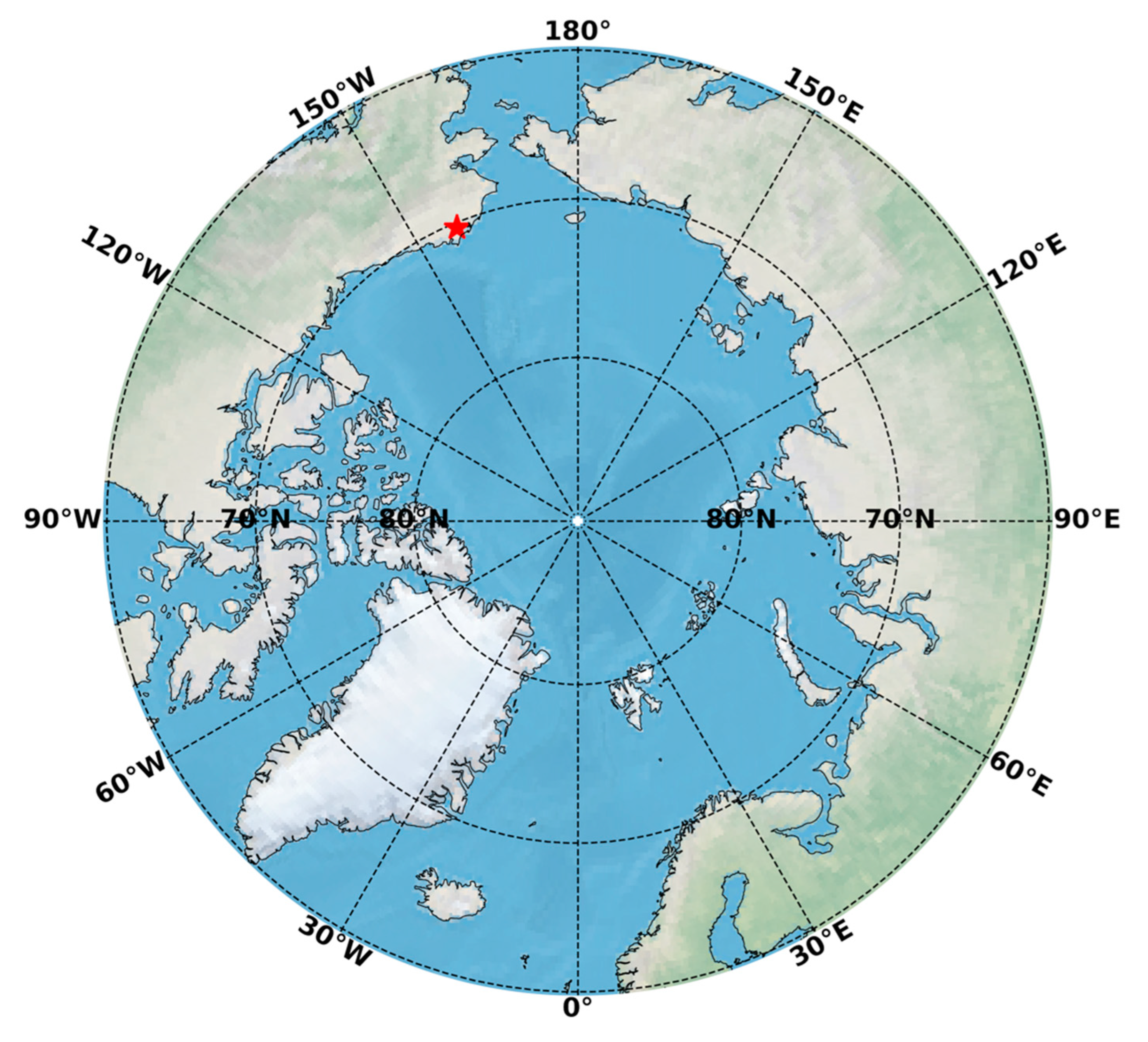
The DOE ARM NSA atmospheric observatory at Utqiaġvik is located on the northern Alaskan coastline (Figure 1). The geolocation of the ARM NSA site was carefully selected to enable observations of complex high-latitude ocean-atmosphere-ice interactions that are poorly represented in climate models. Lacking local topographic obstacles, air masses from local surface and the adjacent Arctic Ocean, and polluted air transported long-range from low latitudes can all strongly influence aerosol physical properties and chemical compositions, and their vertical structures at the NSA site [1,40]. The ARM NSA facility deployed a comprehensive suite of advanced ground-based remote sensing and in situ instruments, including lidars, radars, radiometers, the balloon-borne sounding system (SONDE), and the aerosol observing system to measure aerosol, cloud, precipitation properties, and their impact on atmospheric radiation budget [41,42]. The ARM NSA facility has been collecting continuous data for almost 25 years since 1997, providing critical measurements to study the rapidly changing atmosphere and climate of the Arctic.
HSRL provides separated measurements of molecular and particle signals by taking the advantage of distinct observed Doppler frequency shifts of scattered light caused by molecular velocities and particle motions [43]. Particulate backscatter coefficient () can be absolutely calibrated by reference to the molecular scattering. The molecular scattering profile at a given wavelength of the incident light can be calculated from temperature and pressure profiles measured using SONDE. ARM HSRLs use a narrow field of view receiver of 45 microradians and a narrow optical filter bandwidth of 6 GHz, which effectively reduce the background noise due to scattered sunlight [44]. After careful calibrations, ARM HSRLs provide continuous profiles of , lidar scattering ratio (SR), as well as particulate linear depolarization ratio () at 532 nm with a vertical resolution of 30 m from near the surface to 30 km above the ground level (AGL) and with a temporal resolution of 30 s (https://www.arm.gov/capabilities/instruments/hsrl (accessed on 18 August 2022)). Since at high altitudes lidar signals are usually dominated by background noise (especially the detector noise), we only look at aerosol structures below 8 km. From just molecules () at a given altitude z, SR(z) is the ratio of the total backscatter to the backscatter:
Because using SR can easily identify signals that are larger than that expected from clear air, SR usually is preferred to for the detection of aerosol layers [38]. The ratio of the cross-polarization particulate signal () to the co-polarization particulate signal () at a given altitude z is: .
The depolarization observations allow for robust detection of the presence of irregular particles, such as mineral dust and ice crystals. The ARM HSRL measures particulate depolarizations using circular polarizations. In order to more readily compare our results with previous studies of Arctic aerosol depolarizations, HSRL circular depolarizations are converted to linear depolarizations using the algorithms provided by Flynn et al. [45]. The HSRL at the ARM NSA facility was deployed in April 2011. Because HSRL data between 2011 and 2013 are missing due to instrument issues, we use HSRL measurements from 2014 to 2019 for aerosol analysis in this study.
Table 1 lists the main instruments and their measurements used in this study for analysis at the NSA Utqiaġvik site. An advantage of using the ARM atmospheric observatory facilities is the synergy of HSRL with other instruments. Coincident HSRL and Ka-band ARM Zenith Radar (KAZR) measurements provide the most reliable detection of cloud and precipitation vertical distribution and are used to identify cloud-free conditions. Passive remote sensing instruments, such as the multifilter rotating shadowband radiometer (MFRSR), provide measurements that can be used to retrieve column integrated AODs at 5 narrowband channels of 415, 500, 615, 673, and 870 nm through the Aerosol Optical Depth derived from MFRSR measurement (AOD-MFRSR) value-added product (VAP) (https://www.arm.gov/capabilities/vaps/aod-mfrsr (accessed on 18 August 2022)). Aerosol Ångström exponent (AE) is calculated using AOD () at the 415 and 870 nm wavelength through the equation:
In general, large AE values (e.g., greater than 2) indicate the dominance of small particles in the column and vice versa [46]. It is noted that the up-looking MFRSR measures transported global and diffuse solar irradiances, therefore, MFRSR AOD is only available during the daytime. The SONDE system was launched twice daily, which provides atmospheric pressure, temperature, and humidity profiles. Details of ARM atmospheric observatory instruments can be found on the ARM webpage (https://www.arm.gov/capabilities/instruments (accessed on 18 August 2022)).
To eliminate cloud impacts on aerosol property analysis, cloudy profiles identified from coincident lidar and radar measurements are removed. In this study, we directly use the ARM Active Remote Sensing of Clouds product using Ka-band ARM zenith Radars (KAZRARSCL) VAP (https://www.arm.gov/capabilities/vaps/kazrarscl (accessed on 18 August 2022)) to find cloudy profiles and remove them. In addition, cloud-free profiles that are within 5 min of a cloudy profile are also removed to avoid aerosol wet growth at cloud edges. If a day is too cloudy and cloud-free conditions are less than 10 min, all profiles in the day are removed.
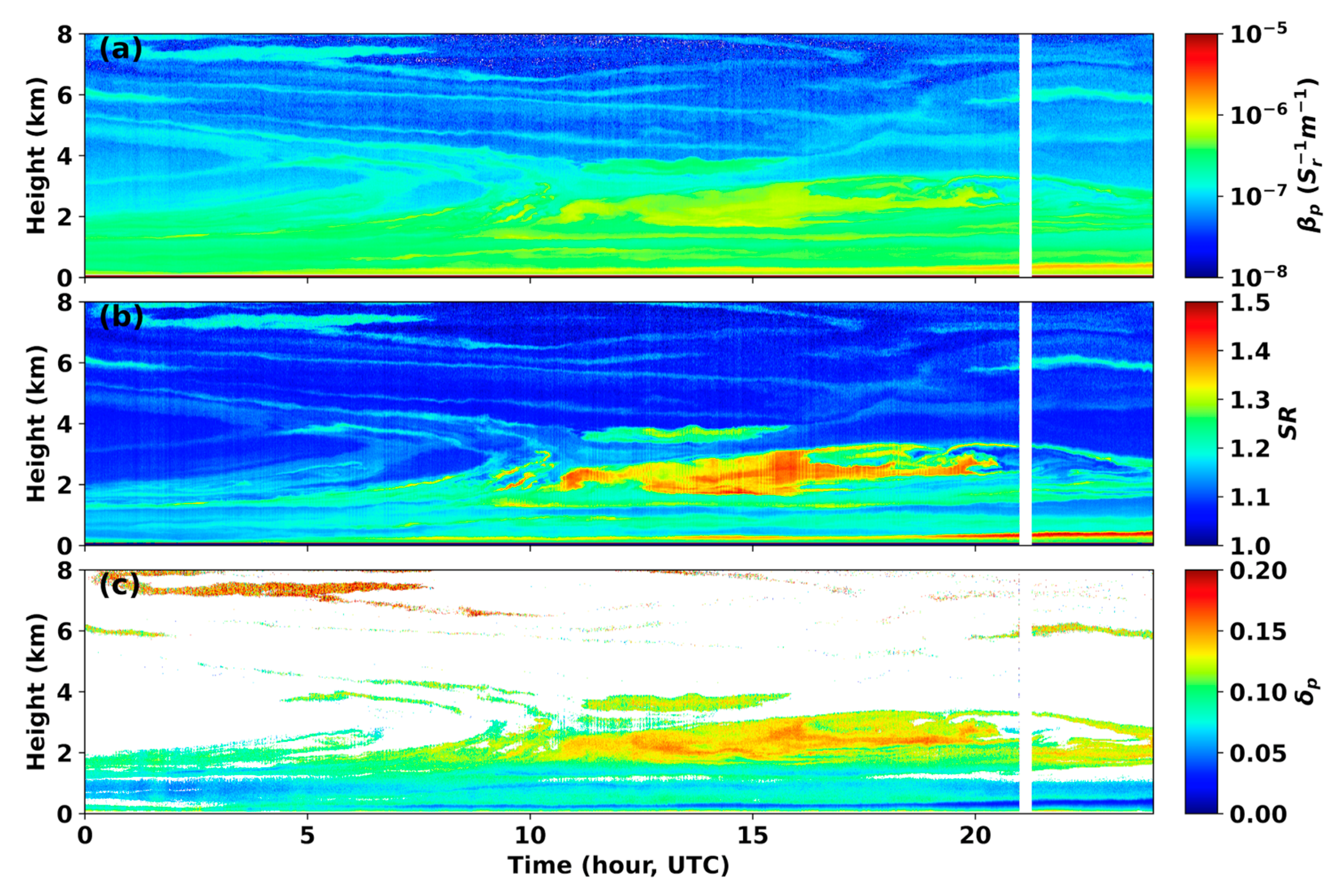
To demonstrate the capability of HSRL for aerosol observations, Figure 2 shows an example of HSRL measurements on 22 March 2016 at the NSA site. From the figure, we can see that multiple aerosol layers are observed from the surface to 8 km. Near the surface, a thin aerosol layer is presented within the boundary layer starting at the 5:00 Coordinated Universal Time (UTC) until the end of the day (Figure 2a,b). Figure 2c shows that this aerosol layer has small , indicating non-depolarizing aerosols are prevalent in the layer. Although there are many fine aerosol structures observed with HSRL measurements, another distinct feature in Figure 2 is the strong elevated aerosol layer from ~2 to 3.5 km between 10:00 and 20:00 UTC and a relatively weaker aerosol layer at ~4 km between 11:00 and 15:00 UTC. Both these two aerosol layers have larger than 0.1, indicating non-spherical aerosol particles, such as mineral dust, dominate the two layers. Other noticeable aerosol layers include the weak aerosol layer between 7 and 8 km from 0:00 to 8:00 UTC and the aerosol layer at ~6 km after 20:00 UTC. Both of them have large , indicating that they are transported dust layers from low-latitude regions. It is also noticed that there are occasionally distinct vertical stripes in HSRL signals that show slightly lower values than the surrounding profiles as can be seen in Figure 2a,b, which might be caused by issues of spectral purity of the laser light or poor temperature control of the iodine cell of the HSRL system. These vertical stripes are not expected to have a dramatic impact on our long-term statistical analysis.
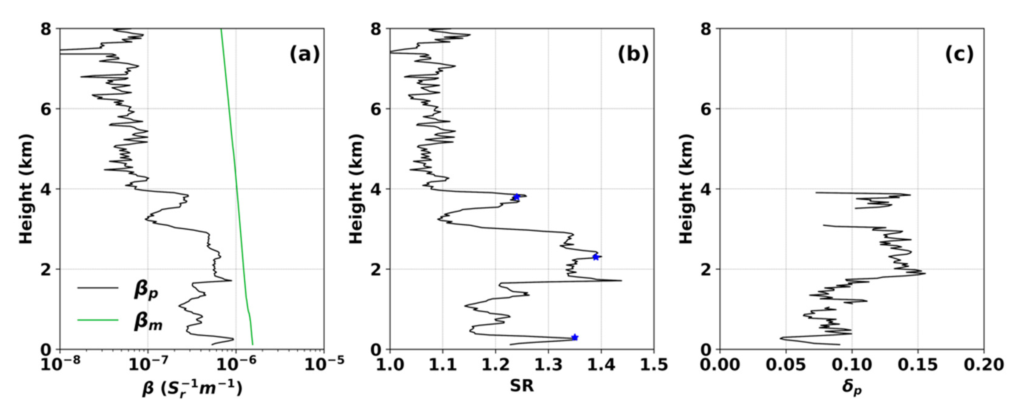
To get a closer look at the values of these variables, Figure 3 presents vertical profiles of HSRL , aerosol SR, and at the 15:00 UTC on the same day. Even for distinct aerosol layers near the surface and at altitudes between 2 and 4 km, is much smaller than . This illustrates the importance of separating molecular and aerosol particulate signals, and the necessity of deploying advanced lidar systems for aerosol observations. SR ranges from 1.0 to 1.45 at different altitudes and the SR profile clearly shows aerosol layers near the surface and at altitudes of ~1, 1.6, 2–3.5 and 3.8 km, while the profile outlines dramatic differences in terms of particle shapes between aerosol layers above and below 2 km. The HYbrid Single-Particle Lagrangian Integrated Trajectory (HYSPLIT, https://www.ready.noaa.gov/HYSPLIT.php (accessed on 18 August 2022)) model of the U.S. National Oceanic and Atmospheric Administration (NOAA) Air Resources Laboratory was used to estimate the sources for the observed aerosol layers. Figure 4 shows the HYSPLIT 20 days backward-trajectories starting at the three altitudes of 0.3, 2.3, and 3.8 km (blue stars in Figure 3) at the NSA site on 22 March 2016, 15:00 UTC. The trajectories point to Southeast Asia as the origin of the aerosol layers at 2.3 and 3.8 km, while Northern Europe was the origin of the aerosol layer at 0.3 km. Large values for aerosol layers at 2.3 and 3.8 km are probably related to prevalent dust events in Southeast Asia in spring [35].
3. Results
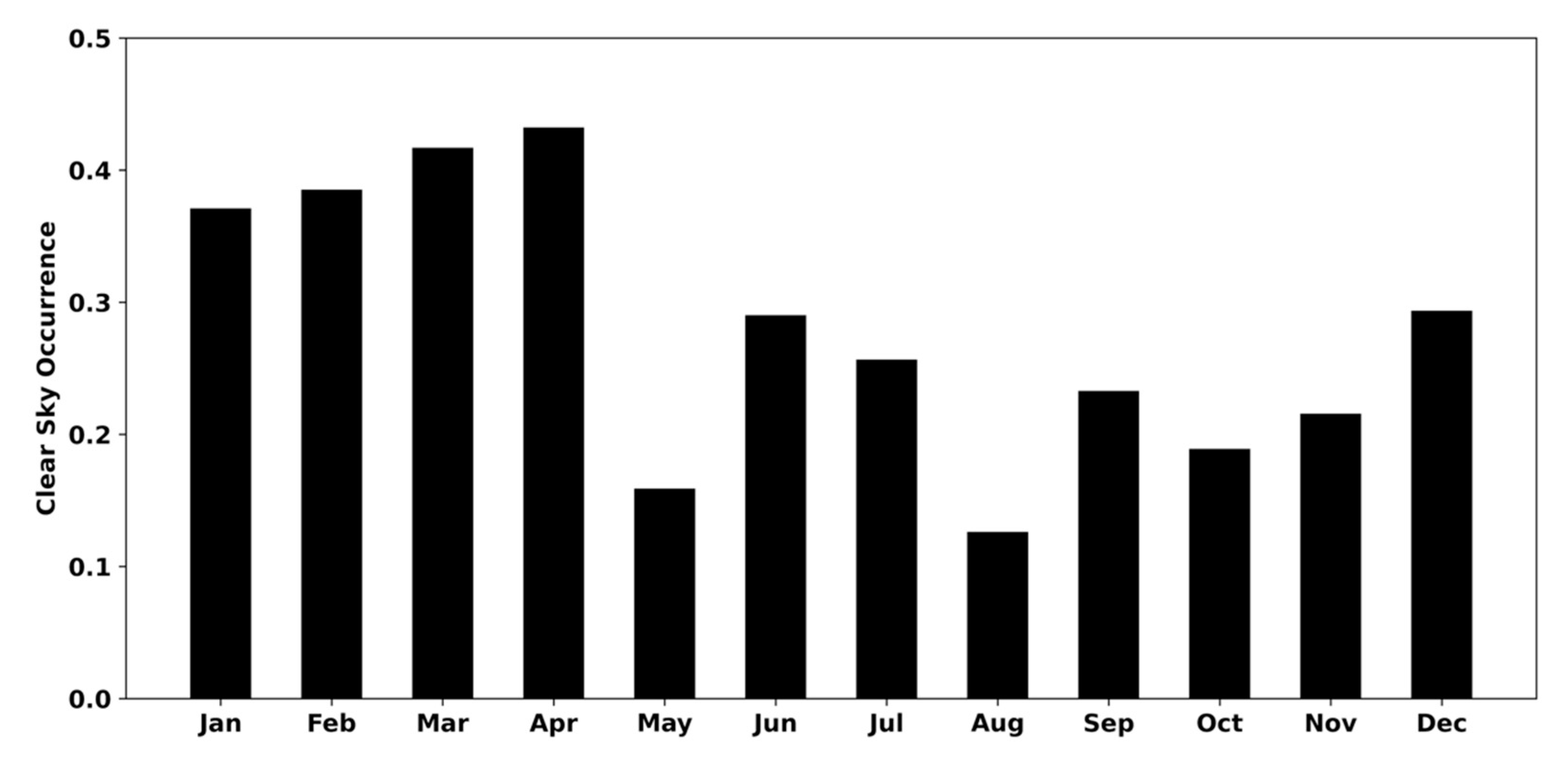
Using 6 years of HSRL data between 2014 and 2019 at the NSA site, in total 490,140 clear sky HSRL profiles were selected for analysis. From the ARM data discovery webpage (https://adc.arm.gov/discovery/#/results/s::nsa%20hsrl (accessed on 18 August 2022)), the ARM HSRL at the NSA observatory was up to provide continuous measurements except between 11 May 2017, and 7 September 2017. HSRL data between 22 November 2017 and 26 April 2018 are marked as ‘suspect’ due to the artifact caused by instrument double-pulsing and are not included in our analysis. Figure 5 shows monthly-mean clear sky occurrences of frequency at the NSA site, which range from 0.13 in August and 0.43 in April. The monthly-mean clear sky occurrence of frequency is derived as the ratio of the number of cloud-free profiles to the number of all profiles at a given month using the ARM KAZRARSCL VAP data. In general, the winter and early spring seasons have higher clear sky occurrences than the summer and fall seasons because persistent low-level clouds are prevalent in the summer and fall seasons [17,49,50].
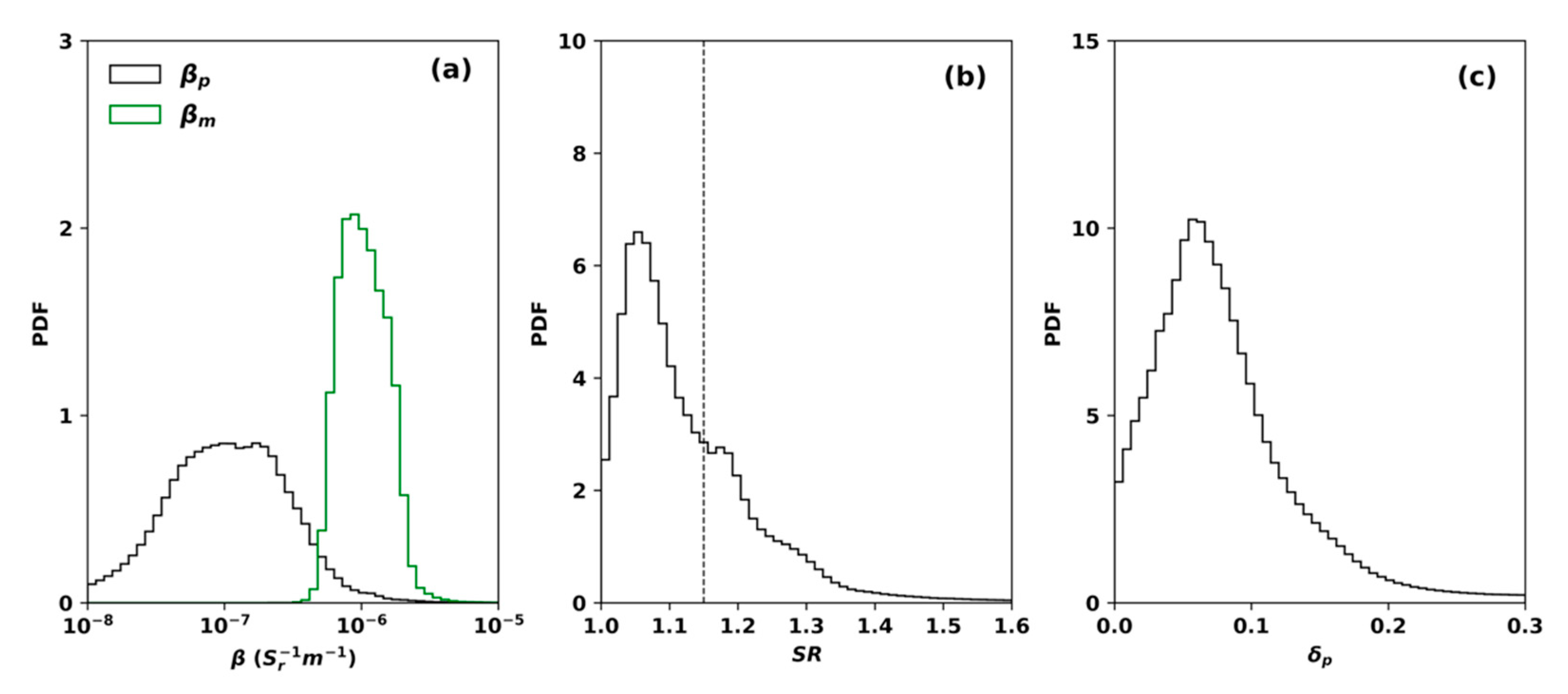
Figure 6 presents the probability distribution function of and , aerosol SR, and between the surface and 8 km. () has an averaged value of 1.6 × (1.2 × ) with a standard deviation of 8.7 × (1.0 × ). In general, is approximately an order of magnitude smaller than at the wavelength of 532 nm. Consistently, SR has an averaged value of 1.13 with a standard deviation of 0.11. The SR distribution shows two peaks at 1.05 and 1.17. From Equation (2), when particulate signals are weak, will be noisy, causing misleading information about aerosol particle shapes. Therefore, we only use of relatively stronger particulate signals for analysis. Considering the two peaks in the SR distribution, we use a threshold value of 1.15 (the dashed line in Figure 5) to separate weak vs. strong particulate signals (referred as ‘weak aerosol layer’ and ‘strong aerosol layer’ correspondingly hereafter) and only include for analysis when SR is above 1.15 through the study. In addition, with negative values or greater than 1 are removed for the analysis. Approximately 28.3% of HSRL pixels have SR above the threshold between the surface and 8 km. has an averaged value of 0.05 with a standard of 0.10.
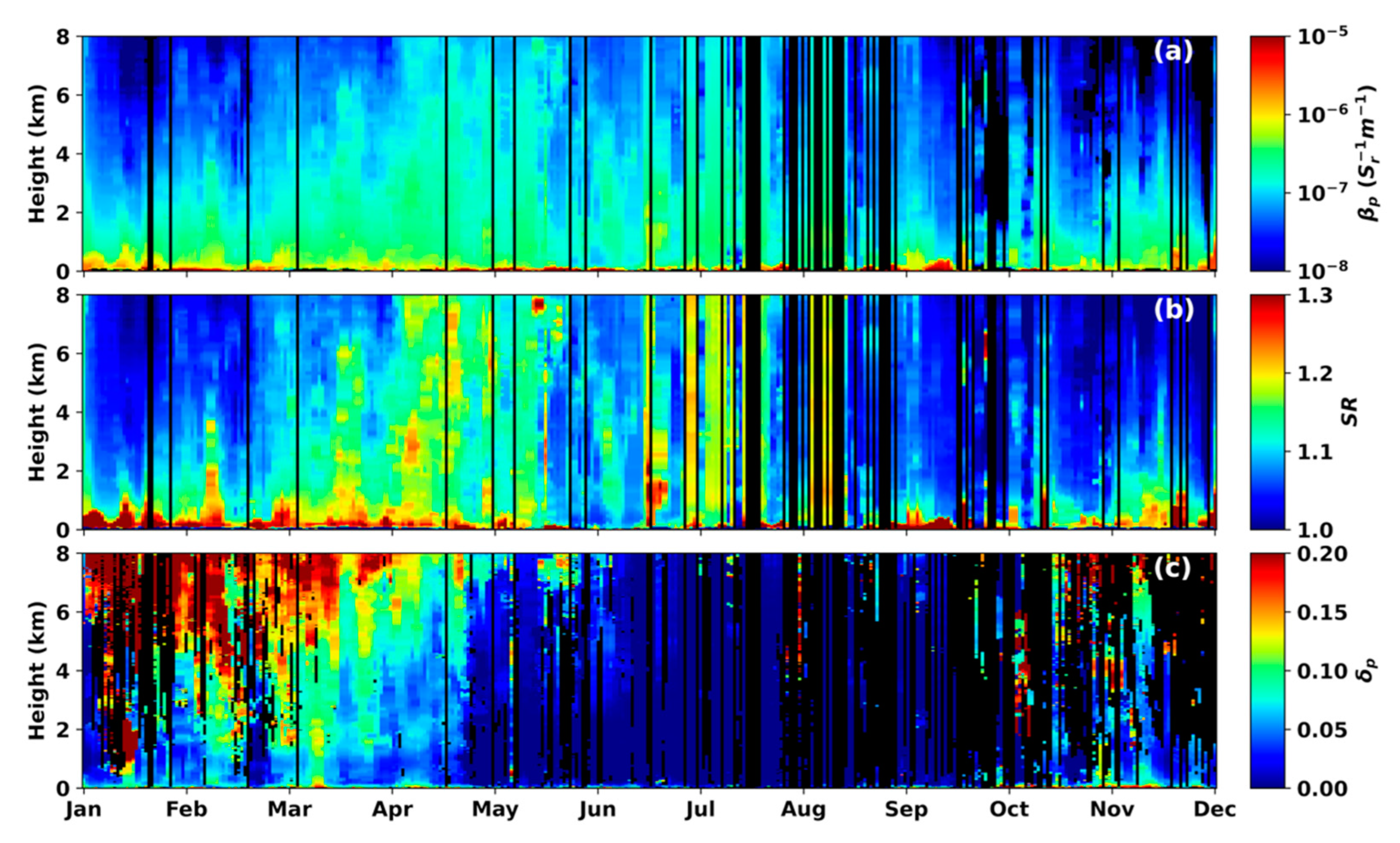
Continuous HSRL observations provide a good opportunity to examine the annual cycle of aerosol vertical distributions. Figure 7 provides daily averaged vertical profiles of , SR, and from the surface to 8 km and their annual cycles. Above 8 km, HSRL signals are much nosier, especially during daytime. We therefore limit our analysis below 8 km. If no cloud-free profiles are found in a given day, the daily-averaged vertical profiles are set to be missing and are shown to be black in the plots. Similarly, if no strong aerosol layers with SR greater than the threshold of 1.15 are found at a given altitude in a day, the daily averaged profiles at the altitude are set to be missing. From Figure 7a,b there is a clear increase of free troposphere aerosol loadings starting in mid-February until May, indicating the prevalence of Arctic Haze in late winter and spring [51]. Interestingly, the Arctic Haze top height also increases from near the surface in mid-February up to 8 km in April and May, as can be seen from Figure 7b. Such variations of Arctic Haze vertical distributions have dramatic impacts on Arctic surface radiative budget and cloud radiative forcing [52]. There are also large aerosol loadings in July and August from the surface up to 8 km with small from Figure 7, which are probably transported marine aerosols from the adjacent Artic Ocean during the summer open-water period [53]. From September to December, free troposphere aerosol loadings are generally low. Figure 7c shows that large are presented above 2 km from January to April and from October to December, indicating the presence of transported mineral dust at the NSA site. Observations of transported dust layers and their impacts on Arctic clouds especially mixed-phase cloud have been investigated by previous studies, e.g., [22,23]. It should be noted that analysis is only applied to strong aerosol layers, therefore, dust embedded in weak aerosol layers are not included in the analysis. Probably because dust particles are mixed with other spherical particles during the long-range transportation, of the Arctic Haze observed in later winter and spring have values generally smaller than 0.1, and are generally small through the whole vertical column from May to September, indicating the dominance of spheric aerosol particles, such as smoke and marine aerosols during this period.
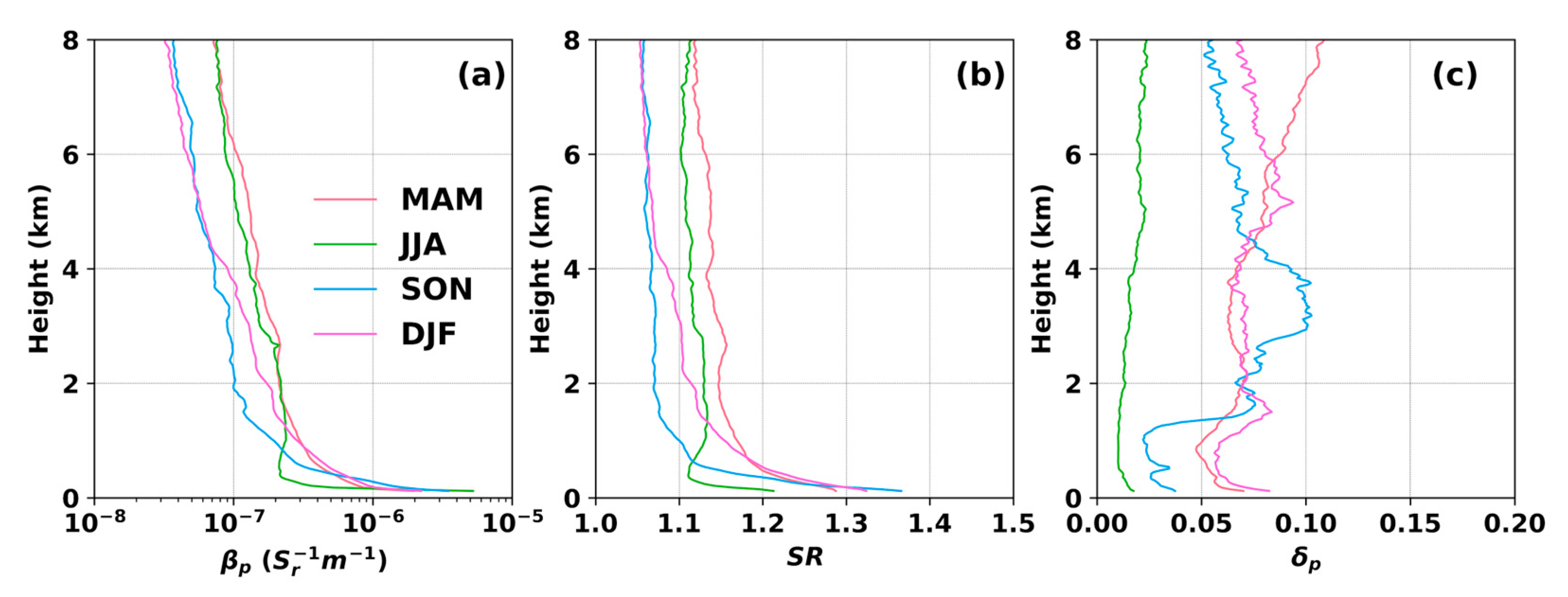
To analyze aerosol variations more quantitatively, Figure 8 shows seasonal mean profiles of , SR, and . From Figure 8a,b, in general both and SR decrease with the altitude. The spring and summer indeed have larger and SR in the free troposphere than the fall and winter seasons. Within the lowest troposphere (e.g., below 1 km), however, summer has the smallest and SR, compared to other seasons. Elevated aerosol layers are occasionally observed above 6 km during the fall season, as shown in both Figure 7a,b and Figure 8a. Figure 8c shows that spring, fall, and winter have larger than the summer season, indicating that mineral dust is frequently presented in strong aerosol layers in these seasons at the NSA site. On the other hand, whether mineral dust is present in weak aerosol layers, is unknown due to the limit of using . The fall profile has larger values in the mid-troposphere between 2 and 4 km, while the winter and spring seasons have larger values at the upper troposphere above 4 km, suggesting mineral dust aerosol layers come from different origins for different seasons.
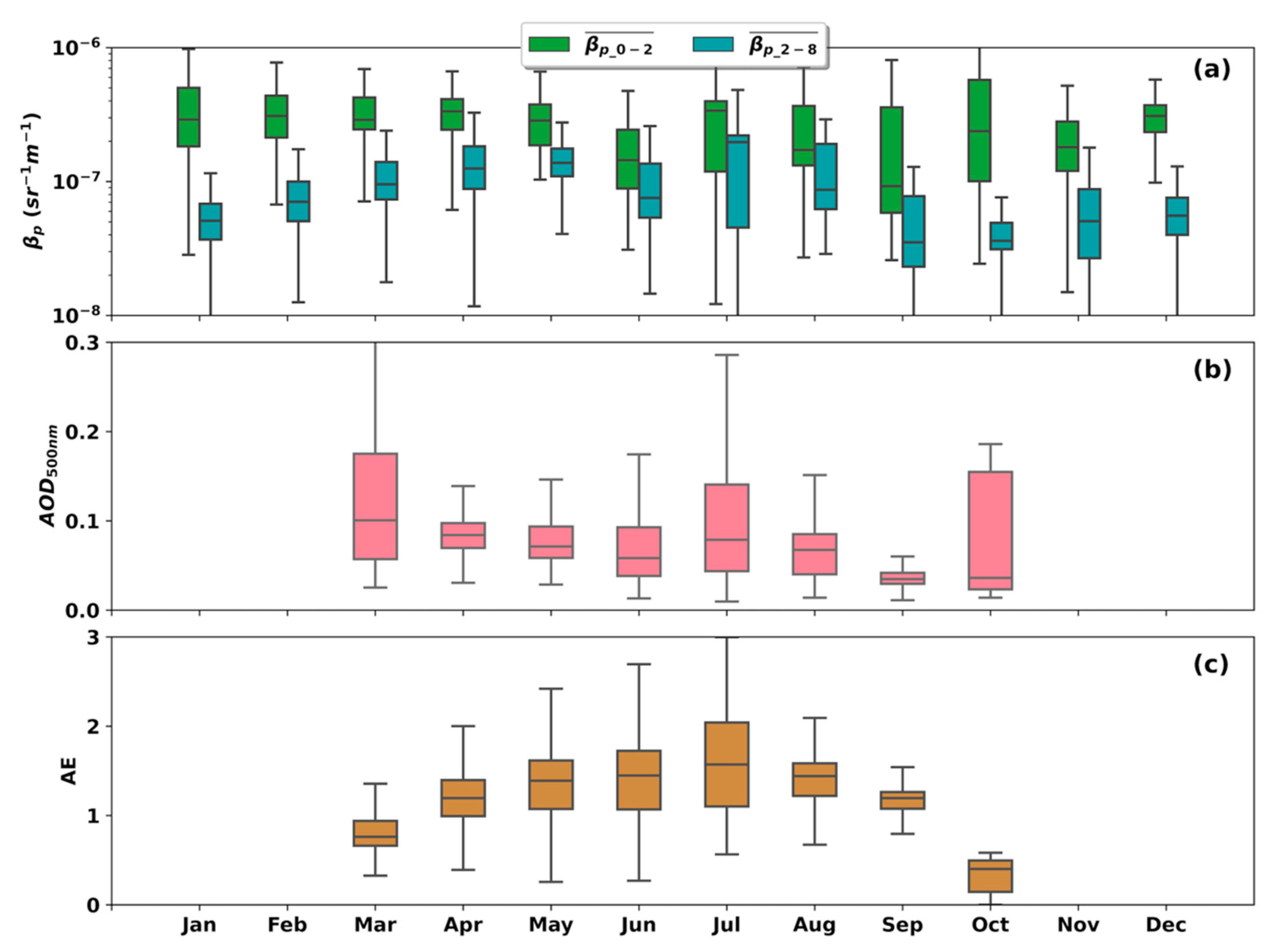
Combined HSRL and passive remote sensing measurements could provide complimentary information on aerosol properties. Figure 9 shows boxplots of monthly distributions of mean between the surface and 2 km () and mean between 2 and 8 km (), MFRSR AOD at the wavelength of 500 nm (AOD500nm), and MFRSR aerosol AE. Considering the challenge to obtain accurate boundary layer height at the NSA site [54], we use a height threshold of 2 km to roughly separate for the lower troposphere and the upper troposphere. From Figure 9a, is smaller in June and September but shows little variations among other months. , on the other hand, shows clear monthly variations with larger values in MAM and JJA and smaller values in SON and DJF, which is consistent with Figure 7 and Figure 8. Figure 9b shows that AOD500nm has larger values in March, July, and October and smaller values in September, a similar monthly variation as , suggesting that low altitude aerosol loadings dominate the AOD at the NSA site. Unfortunately, MFRSR retrievals are not available during the polar night from November to February at the NSA site. Figure 9c shows that AE has a clear monthly variation with larger values in June, July, and August and smaller values in March and October, indicating the dominance of smaller aerosol particles in the summer season and the dominance of large aerosol particles in March and October.
4. Discussion
In this study, analyses using multiple years of HSRL measurements provide an improved understanding of aerosol vertical distributions at the ARM NSA observatory. By effectively separating molecular signals and aerosol particulate signals, HSRL measurements provide unprecedented observations of Arctic aerosol fine structures, as shown in Figure 1. Shibata et al. [36] conducted a similar analysis of Arctic tropospheric aerosol over Ny-Ålesund, Svalbard using two-wavelength elastic scattering lidar at the wavelength of 532 and 1064 nm. In the study, they assumed an extinction-to-backscatter ratio (lidar ratio) of 40 sr to invert lidar signals to get an aerosol backscatter coefficient and a particulate depolarization ratio using the Fernald method [55], which brings an additional uncertainty in Arctic aerosol property analysis. HSRL observed Arctic Haze structures and their annual cycle and the presence of dust particles in strong aerosol layers in the spring, fall, and winter seasons are consistent with previous studies but with higher temporal and vertical resolutions [56,57,58].
The dataset and analyses presented in this study can be readily used to validate model simulations of Arctic aerosol distributions, especially for those with lidar simulators. Climate models have difficulty reproducing seasonal variations of Artic aerosol distributions due to the lack of observational constraints on aerosol wet and dry removal processes [59]. Ground-based and spaceborne lidar observations have been used to validate simulated aerosol concentrations over the Arctic region by comparing lidar-observed with calculated from model outputs together with a lidar simulator [60]. The annual cycle and seasonal variations of presented in this study can be directly used to compare with model simulations. The analyses of aerosol vertical distribution can also be used to improve the understanding of complex cloud-aerosol interactions over the Arctic region [17]. Aerosol layers presented at different altitudes could exert different impacts on Arctic clouds [61]. The vertical structures of Arctic Haze and dust-containing aerosol layers from HSRL measurements provide a good dataset that can be used to study aerosol impact on long-persistent mixed-phase clouds at the NSA site [62,63].
HSRL measurements can also be used to derive particulate extinction coefficient profiles from the measured molecular signals [43]. However, HSRL photon counting noise and imprecise overlap function corrections at the near range could cause large uncertainties in the derived particulate extinction coefficient when the signal-to-noise ratio is small. Eloranta [43] suggested that HSRL provides useful particulate extinction coefficient estimation when the extinction exceeds ~10−4 m−1. Considering that Arctic aerosol loadings are often lower than this threshold and large uncertainties in particulate extinction coefficient estimations could dramatically impact statistical analysis results, we did not include particulate extinction coefficient in our analysis in this study. It is also noted that single-wavelength lidars have their limits and are not able to provide aerosol microphysical property retrievals. Multi-wavelength lidar measurements using three backscatter channels plus two extinction channels could be used to provide retrievals of aerosol microphysical property profiles including aerosol effective radius, total number concentration, and complex refractive index [64,65]. Deployment of advanced multi-wavelength lidar systems at polar regions is needed to further improve the understanding of aerosol processes and their impacts on cloud properties.
A limitation of ground-based remote sensing measurements at a given observatory is that they only cover a small region. There could be large spatial variations of aerosol vertical distributions across the entire Arctic region. Mobile facilities carrying advanced remote sensing instruments could alleviate this limitation. Recently, two advanced lidars, including RL and HSRL, were onboard the drifting Polarstern during the Multidisciplinary drifting Observatory for the Study of Arctic Climate expedition (MOSAiC), providing explicit aerosol vertical distribution measurements over the Central Arctic [59,66]. Spaceborne lidars onboard a polar-orbiting satellite, such as the Lidar In-space Technology Experiment (LITE) and CALIOP, provide aerosol three dimensional distributions on a global scale [67]. In the near future, the first space-borne HSRL will be launched during the Cloud, Aerosol, and Radiation Explorer (EarthCARE) mission, which will provide more reliable atmospheric aerosol distributions over the polar regions [68].
5. Conclusions
Aerosol vertical distributions dramatically impact both aerosol direct and indirect radiative effects. Advanced lidar systems, such as the High Spectra Resolution Lidar (HSRL) and Raman Lidar (RL), can effectively separate atmospheric molecular signals and aerosol particle signals, which provide reliable measurements of aerosol properties over the Arctic regions. We use 6 years of HSRL measurements from the Department of Energy (DOE) Atmospheric Radiation Measurement (ARM) North Slope of Alaska (NSA) atmospheric observatory at Utqiaġvik to analyze Arctic aerosol vertical distributions. We focus our analysis on aerosol particulate backscatter coefficient (), lidar scattering ratio (SR), and aerosol particulate depolarization ratio () profiles. The main findings are listed below.
- (1)
- A case study on 22 March 2016 at the NSA site shows that HSRL is able to observe fine aerosol vertical distributions. Aerosol layers at different altitudes have different origins according to the National Oceanic and Atmospheric Administration (NOAA) HYbrid Single-Particle Lagrangian Integrated Trajectory (HYSPLIT) back trajectory model simulations;
- (2)
- Probability Distribution Functions (PDFs) of , SR, and from 6 years of HSRL data confirm that is generally one order of magnitude smaller than atmospheric molecular scatter (). Considering that is noisy when lidar signals are weak, we use a SR threshold value of 1.15 to separate weak aerosol layers and strong aerosol layers; is only analyzed when SR is above 1.15 through the study;
- (3)
- The annual cycle of aerosol vertical distributions shows that Arctic Haze events are frequently observed in later winter and spring at the NSA site. Top heights of the Arctic Haze increase from near the surface in February to 8 km in April and May. Large aerosol loadings with small are observed in July and August, which could be caused by transported marine aerosols from the adjacent Artic Ocean during the open-water period. In addition, mineral dust is frequently presented in strong aerosol layers in the spring, fall, and winter seasons at the NSA site;
- (4)
- Combined HSRL and multifilter rotating shadowband radiometer (MFRSR) data show that aerosol optical depth (AOD) at the wavelength of 500 nm have similar monthly variations with low altitude aerosol loading. MFRSR derived aerosol Ångström exponent (AE) between the 415 and 870 nm shows larger values in June, July, and August, and smaller values in March and October, indicating the dominance of smaller aerosol particles in the summer season and the dominance of large aerosol particles in March and October.
Author Contributions
Conceptualization, D.Z. and Z.W.; methodology, D.Z.; software, D.Z.; validation, D.Z.; formal analysis, D.Z., Z.W., J.C. and H.X.; investigation, D.Z.; resources, D.Z.; data curation, D.Z.; writing—original draft preparation, D.Z.; writing—review and editing, J.C., H.X. and Z.W.; visualization, D.Z.; supervision, D.Z.; project administration, D.Z.; funding acquisition, J.C. All authors have read and agreed to the published version of the manuscript.
Funding
D.Z. and J.C. were supported by the U.S. Department of Energy (DOE) Atmospheric Radiation Measurement (ARM) Program (grant no. DE-AC05-76RL01830). H.X. and Z.W. were supported by the U.S. DOE Atmospheric System Research (ASR) Program (grant no. DE-SC0020510).
Data Availability Statement
The HSRL, KAZR-ARSCL, SONDE, and MFRSR data used in this study can be freely downloaded from the ARM data archive site: https://www.archive.arm.gov/discovery/ (accessed on 18 August 2022).
Acknowledgments
We thank the personnel responsible for the challenging operations and data collection for the ARM NSA observatories at Utqiaġvik. Data were obtained from the Atmospheric Radiation Measurement (ARM) user facility, a U.S. Department of Energy (DOE) office of science user facility managed by the Biological and Environmental Research (BER) program. The authors also want to thank the anonymous reviewers for their helpful comments in improving the manuscript.
Conflicts of Interest
The authors declare no conflict of interest.
References
- Curry, J.A.; Schramm, J.L.; Rossow, W.B.; Randall, D. Overview of Arctic Cloud and Radiation Characteristics. J. Clim. 1996, 9, 1731–1764. [Google Scholar] [CrossRef]
- Lubin, D.; Vogelmann, A.M. A climatologically significant aerosol longwave indirect effect in the Arctic. Nature 2006, 439, 453–456. [Google Scholar] [CrossRef]
- Wang, Y.; Jiang, J.H.; Su, H.; Choi, Y.; Huang, L.; Guo, J.; Yung, Y.L. Elucidating the Role of Anthropogenic Aerosols in Arctic Sea Ice Variations. J. Clim. 2018, 31, 99–114. [Google Scholar] [CrossRef]
- Polyakov, I.V.; Alekseev, G.V.; Bekryaev, R.V.; Bhatt, U.; Colony, R.; Johnson, M.A.; Karklin, V.P.; Makshtas, A.P.; Walsh, D.; Yulin, A.V. Observationally based assessment of polar amplification of global warming. Geophys. Res. Lett. 2002, 29, 1878. [Google Scholar] [CrossRef]
- Holland, M.M.; Bitz, C.M. Polar amplification of climate change in coupled models. Clim. Dyn. 2003, 21, 221–232. [Google Scholar] [CrossRef]
- Previdi, M.; Smith, K.L.; Polvani, L.M. Arctic amplification of climate change: A review of underlying mechanisms. Environ. Res. Lett. 2021, 16, 093003. [Google Scholar] [CrossRef]
- Schuur, E.A.G.; McGuire, A.D.; Schädel, C.; Grosse, G.; Harden, J.W.; Hayes, D.J.; Hugelius, G.; Koven, C.D.; Kuhry, P.; Lawrence, D.M.; et al. Climate change and the permafrost carbon feedback. Nature 2015, 520, 171–179. [Google Scholar] [CrossRef]
- Screen, J.A.; Deser, C.; Simmonds, I. Local and remote controls on observed Arctic warming. Geophys. Res. Lett. 2012, 39, L10709. [Google Scholar] [CrossRef]
- England, M.R.; Eisenman, I.; Lutsko, N.J.; Wagner, T.J. The recent emergence of Arctic Amplification. Geophys. Res. Lett. 2021, 48, e2021GL094086. [Google Scholar] [CrossRef]
- Schmale, J.; Zieger, P.; Ekman, A.M. Aerosols in current and future Arctic climate. Nat. Clim. Chang. 2021, 11, 95–105. [Google Scholar] [CrossRef]
- Bellouin, N.; Boucher, O.; Haywood, J.; Reddy, M.S. Global estimate of aerosol direct radiative forcing from satellite measurements. Nature 2005, 438, 1138–1141. [Google Scholar] [CrossRef]
- Lohmann, U.; Feichter, J. Global indirect aerosol effects: A review. Atmospheric Chem. Phys. 2005, 5, 715–737. [Google Scholar] [CrossRef]
- Breider, T.J.; Mickley, L.J.; Jacob, D.J.; Ge, C.; Wang, J.; Sulprizio, M.P.; Croft, B.; Ridley, D.A.; McConnell, J.R.; Sharma, S.; et al. Multidecadal Trends in Aerosol Radiative Forcing over the Arctic: Contribution of Changes in Anthropogenic Aerosol to Arctic Warming since 1980. J. Geophys. Res. Atmos. 2017, 122, 3573–3594. [Google Scholar] [CrossRef]
- Garrett, T.J.; Zhao, C.; Dong, X.; Mace, G.G.; Hobbs, P.V. Effects of varying aerosol regimes on low-level Arctic stratus. Geophys. Res. Lett. 2004, 31, L17105. [Google Scholar] [CrossRef]
- Lubin, D.; Vogelmann, A. Observational quantification of a total aerosol indirect effect in the Arctic. Tellus B Chem. Phys. Meteorol. 2010, 62, 181–189. [Google Scholar] [CrossRef]
- Mauritsen, T.; Sedlar, J.; Tjernström, M.; Leck, C.; Martin, M.; Shupe, M.; Sjogren, S.; Sierau, B.; Persson, P.O.G.; Brooks, I.M.; et al. An Arctic CCN-limited cloud-aerosol regime. Atmos. Chem. Phys. 2011, 11, 165–173. [Google Scholar] [CrossRef]
- Morrison, H.; de Boer, G.; Feingold, G.; Harrington, J.; Shupe, M.D.; Sulia, K. Resilience of persistent Arctic mixed-phase clouds. Nat. Geosci. 2012, 5, 11–17. [Google Scholar] [CrossRef]
- Solomon, A.; Feingold, G.; Shupe, M.D. The role of ice nuclei recycling in the maintenance of cloud ice in Arctic mixed-phase stratocumulus. Atmos. Chem. Phys. 2015, 15, 10631–10643. [Google Scholar] [CrossRef]
- Shupe, M.D.; Daniel, J.S.; de Boer, G.; Eloranta, E.W.; Kollias, P.; Long, C.N.; Luke, E.P.; Turner, D.D.; Verlinde, J. A Focus On Mixed-Phase Clouds. Bull. Am. Meteorol. Soc. 2008, 89, 1549–1562. [Google Scholar] [CrossRef]
- Zhao, M.; Wang, Z. Comparison of Arctic clouds between European Center for Medium-Range Weather Forecasts simulations and Atmospheric Radiation Measurement Climate Research Facility long-term observations at the North Slope of Alaska Barrow site. J. Geophys. Res. Earth Surf. 2010, 115, D23202. [Google Scholar] [CrossRef]
- Fan, J.; Ghan, S.; Ovchinnikov, M.; Liu, X.; Rasch, P.J.; Korolev, A. Representation of Arctic mixed-phase clouds and the Wegener-Bergeron-Findeisen process in climate models: Perspectives from a cloud-resolving study. J. Geophys. Res. Earth Surf. 2011, 116, D00T07. [Google Scholar] [CrossRef]
- Zhang, D.; Wang, Z.; Kollias, P.; Vogelmann, A.M.; Yang, K.; Luo, T. Ice particle production in mid-level stratiform mixed-phase clouds observed with collocated A-Train measurements. Atmos. Chem. Phys. 2018, 18, 4317–4327. [Google Scholar] [CrossRef]
- Shi, Y.; Liu, X.; Wu, M.; Zhao, X.; Ke, Z.; Brown, H. Relative importance of high-latitude local and long-range-transported dust for Arctic ice-nucleating particles and impacts on Arctic mixed-phase clouds. Atmos. Chem. Phys. 2022, 22, 2909–2935. [Google Scholar] [CrossRef]
- Sterzinger, L.J.; Sedlar, J.; Guy, H.; Neely, R.R., III; Igel, A.L. Do Arctic mixed-phase clouds sometimes dissipate due to insufficient aerosol? Evidence from comparisons between observations and idealized simulations. Atmos. Chem. Phys. 2022, 22, 8973–8988. [Google Scholar] [CrossRef]
- Lohmann, U.; Hoose, C. Sensitivity studies of different aerosol indirect effects in mixed-phase clouds. Atmos. Chem. Phys. 2009, 9, 8917–8934. [Google Scholar] [CrossRef]
- Wang, Y.; Zheng, X.; Dong, X.; Xi, B.; Wu, P.; Logan, T.; Yung, Y.L. Impacts of long-range transport of aerosols on marine-boundary-layer clouds in the eastern North Atlantic. Atmos. Chem. Phys. 2020, 20, 14741–14755. [Google Scholar] [CrossRef]
- Quinn, P.K.; Bates, T.S.; Schulz, K.; Shaw, G.E. Decadal trends in aerosol chemical composition at Barrow, Alaska: 1976–2008. Atmos. Chem. Phys. 2009, 9, 8883–8888. [Google Scholar] [CrossRef]
- Dall’Osto, M.; Beddows, D.C.S.; Tunved, P.; Harrison, R.M.; Lupi, A.; Vitale, V.; Becagli, S.; Traversi, R.; Park, K.-T.; Yoon, Y.J.; et al. Simultaneous measurements of aerosol size distributions at three sites in the European high Arctic. Atmos. Chem. Phys. 2019, 19, 7377–7395. [Google Scholar] [CrossRef]
- Thomas, M.A.; Devasthale, A.; Tjernström, M.; Ekman, A.M.L. The relation between aerosol vertical distribution and temperature inversions in the arctic in winter and spring. Geophys. Res. Lett. 2019, 46, 2836–2845. [Google Scholar] [CrossRef]
- McFarquhar, G.M.; Ghan, S.; Verlinde, J.; Korolev, A.; Strapp, J.W.; Schmid, B.; Tomlinson, J.M.; Wolde, M.; Brooks, S.D.; Cziczo, D.; et al. Indirect and Semi-Direct Aerosol Campaign: The Impact of Arctic Aerosols on Clouds. Bull. Am. Meteorol. Soc. 2011, 92, 183–201. [Google Scholar] [CrossRef] [Green Version]
- Wendisch, M.; Macke, A.; Ehrlich, A.; Lüpkes, C.; Mech, M.; Chechin, D.; Dethloff, K.; Velasco, C.B.; Bozem, H.; Brückner, M.; et al. The Arctic Cloud Puzzle: Using ACLOUD/PASCAL Multiplatform Observations to Unravel the Role of Clouds and Aerosol Particles in Arctic Amplification. Bull. Am. Meteorol. Soc. 2019, 100, 841–871. [Google Scholar] [CrossRef]
- Kabanov, D.M.; Ritter, C.; Sakerin, S.M. Interannual and seasonal variations in the aerosol optical depth of the atmosphere in two regions of Spitsbergen (2002–2018). Atmos. Meas. Tech. 2020, 13, 5303–5317. [Google Scholar] [CrossRef]
- Kassianov, E.; Pekour, M.; Barnard, J.; Flynn, C.J.; Mei, F.; Berg, L.K. Estimation of Aerosol Columnar Size Distribution from Spectral Extinction Data in Coastal and Maritime Environment. Atmosphere 2021, 12, 1412. [Google Scholar] [CrossRef]
- Winker, D.M.; Pelon, J.; Coakley, J.A., Jr.; Ackerman, S.A.; Charlson, R.J.; Colarco, P.R.; Flamant, P.; Fu, Q.; Hoff, R.; Kittaka, C.; et al. The CALIPSO mission: A global 3D view of aerosols and clouds. Bull. Am. Meteorol. Soc. 2010, 91, 1211–1229. [Google Scholar] [CrossRef]
- Yang, K.; Wang, Z.; Luo, T.; Liu, X.; Wu, M. Upper troposphere dust belt formation processes vary seasonally and spatially in the Northern Hemisphere. Commun. Earth Environ. 2022, 3, 24. [Google Scholar] [CrossRef]
- Shibata, T.; Shiraishi, K.; Shiobara, M.; Iwasaki, S.; Takano, T. Seasonal variations in high arctic free tropospheric aerosols over ny-ålesund, svalbard, observed by ground-based lidar. J. Geophys. Res. Atmos. 2018, 123, 12353–12367. [Google Scholar] [CrossRef]
- Eloranta, E.; Ponsardin, P. A High Spectral Resolution Lidar Designed for Unattended Operation in the Arctic; Optica Publishing Group: Coeur d’Alene, ID, USA, 2001. [Google Scholar]
- Thorsen, T.J.; Fu, Q.; Newsom, R.K.; Turner, D.; Comstock, J. Automated Retrieval of Cloud and Aerosol Properties from the ARM Raman Lidar. Part I: Feature Detection. J. Atmos. Ocean. Technol. 2015, 32, 1977–1998. [Google Scholar] [CrossRef]
- Thorsen, T.; Fu, Q. Automated Retrieval of Cloud and Aerosol Properties from the ARM Raman Lidar. Part II: Extinction. J. Atmos. Ocean. Technol. 2015, 32, 1999–2023. [Google Scholar] [CrossRef]
- Garrett, T.J.; Zhao, C. Increased Arctic cloud longwave emissivity associated with poullution from mid-latitudes. Nature 2006, 440, 787–789. [Google Scholar] [CrossRef]
- Mather, J.H.; Voyles, J.W. The Arm Climate Research Facility: A Review of Structure and Capabilities. Bull. Am. Meteorol. Soc. 2013, 94, 377–392. [Google Scholar] [CrossRef]
- Verlinde, J.; Zak, B.D.; Shupe, M.D.; Ivey, M.D.; Stamnes, K. The ARM North Slope of Alaska (NSA) Sites. Meteorol. Monogr. 2016, 57, 8.1–8.13. [Google Scholar] [CrossRef]
- Eloranta, E. High Spectral Resolution lidar measurements of atmospheric extinction: Progress and challenges. In Proceedings of the 2014 IEEE Aerospace Conference, Big Sky, MT, USA, 1–8 March 2014; pp. 1–6. [Google Scholar] [CrossRef]
- Goldsmith, J. High Spectral Resolution Lidar (HSRL) Instrument Handbook; No. DOE/SC-ARM-TR-157; DOE Office of Science Atmospheric Radiation Measurement (ARM) Program (United States): Albuquerque, NM, USA, 2016. [Google Scholar] [CrossRef]
- Flynn, C.J.; Mendoza, A.; Zheng, Y.; Mathur, S. Novel polarization-sensitive micropulse lidar measurement technique. Opt. Express 2007, 15, 2785–2790. [Google Scholar] [CrossRef]
- Schuster, G.L.; Dubovik, O.; Holben, B.N. Angstrom exponent and bimodal aerosol size distributions. J. Geophys. Res. Earth Surf. 2006, 111, D07207. [Google Scholar] [CrossRef]
- Eloranta, E.W. High Spectral Resolution Lidar. In Lidar: Range-Resolved Optical Remote Sensing of the Atmosphere; Weitkamp, K., Ed.; Springer Series in Optical Sciences; Springer: New York, NY, USA, 2005; pp. 143–163. [Google Scholar]
- Kollias, P.; Clothiaux, E.E.; Ackerman, T.P.; Albrecht, B.A.; Widener, K.B.; Moran, K.P.; Luke, E.; Johnson, K.L.; Bharadwaj, N.; Mead, J.B.; et al. Development and Applications of ARM Millimeter-Wavelength Cloud Radars. Meteorol. Monogr. 2016, 57, 17.1–17.19. [Google Scholar] [CrossRef]
- Shupe, M.D.; Matrosov, S.; Uttal, T. Arctic Mixed-Phase Cloud Properties Derived from Surface-Based Sensors at SHEBA. J. Atmos. Sci. 2006, 63, 697–711. [Google Scholar] [CrossRef]
- Shupe, M.D.; Turner, D.D.; Zwink, A.; Thieman, M.M.; Mlawer, E.J.; Shippert, T. Deriving Arctic Cloud Microphysics at Barrow, Alaska: Algorithms, Results, and Radiative Closure. J. Appl. Meteorol. Climatology 2015, 54, 1675–1689. [Google Scholar] [CrossRef]
- Shaw, G.E. The Arctic Haze Phenomenon. Bull. Am. Meteorol. Soc. 1995, 76, 2403–2414. [Google Scholar] [CrossRef]
- Zhao, C.; Garrett, T.J. Effects of Arctic haze on surface cloud radiative forcing. Geophys. Res. Lett. 2015, 42, 557–564. [Google Scholar] [CrossRef]
- Moffett, C.E.; Barrett, T.E.; Liu, J.; Gunsch, M.J.; Upchurch, L.M.; Quinn, P.K.; Pratt, K.A.; Sheesley, R.J. Long-Term Trends for Marine Sulfur Aerosol in the Alaskan Arctic and Relationships With Temperature. J. Geophys. Res. Atmos. 2020, 125, e2020JD033225. [Google Scholar] [CrossRef]
- Zhang, D.; Comstock, J.; Morris, V. Comparisons of Planetary Boundary Layer Height from Ceilometer with ARM Radiosonde Data. Atmospheric Meas. Tech. 2022, 15, 4735–4749. [Google Scholar] [CrossRef]
- Fernald, F.G. Analysis of atmospheric lidar observations: Some comments. Appl. Opt. 1984, 23, 652–653. [Google Scholar] [CrossRef] [PubMed]
- Ishii, S.; Shibata, T.; Nagai, T.; Mizutani, K.; Itabe, T.; Hirota, M.; Fujimoto, T.; Uchino, O. Arctic haze and clouds observed by lidar during four winter seasons of 1993–1997, at Eureka, Canada. Atmos. Environ. 1999, 33, 2459–2470. [Google Scholar] [CrossRef]
- Quinn, P.K.; Shaw, G.; Andrews, E.; Dutton, E.G.; Ruoho-Airola, T.; Gong, S.L. Arctic haze: Current trends and knowledge gaps. Tellus B: Chem. Phys. Meteorol. 2007, 59, 99–114. [Google Scholar] [CrossRef]
- Luo, T.; Wang, Z.; Zhang, D.; Liu, X.; Wang, Y.; Yuan, R. Global dust distribution from improved thin dust layer detection using A-train satellite lidar observations. Geophys. Res. Lett. 2015, 42, 620–628. [Google Scholar] [CrossRef]
- Textor, C.; Schulz, M.; Guibert, S.; Kinne, S.; Balkanski, Y.; Bauer, S.; Berntsen, T.; Berglen, T.; Boucher, O.; Chin, M.; et al. Analysis and quantification of the diversities of aerosol life cycles within AeroCom Atmos. Chem. Phys. 2006, 6, 1777–1813. [Google Scholar]
- Bourgeois, Q.; Bey, I. Pollution transport efficiency toward the Arctic: Sensitivity to aerosol scavenging and source regions. J. Geophys. Res. Earth Surf. 2011, 116, D08213. [Google Scholar] [CrossRef]
- Engelmann, R.; Ansmann, A.; Ohneiser, K.; Griesche, H.; Radenz, M.; Hofer, J.; Althausen, D.; Dahlke, S.; Maturilli, M.; Veselovskii, I.; et al. Wildfire Smoke, Arctic Haze, and Aerosol Effects on Mixed-Phase and Cirrus Clouds over the North Pole Region during MOSAiC: An Introduction. Atmos. Chem. Phys. 2021, 21, 13397–13423. [Google Scholar] [CrossRef]
- Zhang, D.; Wang, Z.; Heymsfield, A.; Fan, J.; Liu, D.; Zhao, M. Quantifying the impact of dust on heterogeneous ice generation in midlevel supercooled stratiform clouds. Geophys. Res. Lett. 2012, 39, L18805. [Google Scholar] [CrossRef]
- Kalesse, H.; de Boer, G.; Solomon, A.; Oue, M.; Ahlgrimm, M.; Zhang, D.; Shupe, M.D.; Luke, E.; Protat, A. Understanding Rapid Changes in Phase Partitioning between Cloud Liquid and Ice in Stratiform Mixed-Phase Clouds: An Arctic Case Study. Mon. Weather Rev. 2016, 144, 4805–4826. [Google Scholar] [CrossRef]
- Burton, S.P.; Chemyakin, E.; Liu, X.; Knobelspiesse, K.; Stamnes, S.; Sawamura, P.; Moore, R.H.; Hostetler, C.A.; Ferrare, R.A. Information content and sensitivity of the 3β + 2α lidar measurement system for aerosol microphysical retrievals. Atmos. Meas. Tech. 2016, 9, 5555–5574. [Google Scholar] [CrossRef]
- McLean, W.G.K.; Fu, G.; Burton, S.P.; Hasekamp, O.P. Retrieval of aerosol microphysical properties from atmospheric lidar sounding: An investigation using synthetic measurements and data from the ACEPOL campaign. Atmos. Meas. Tech. 2021, 14, 4755–4771. [Google Scholar] [CrossRef]
- Shupe, M.D.; Rex, M.; Blomquist, B.; Persson, P.O.G.; Schmale, J.; Uttal, T.; Althausen, D.; Angot, H.; Archer, S.; Bariteau, L.; et al. Overview of the MOSAiC expedition: Atmosphere. Elementa Sci. Anthr. 2022, 10, 60. [Google Scholar] [CrossRef]
- Winker, D.M.; Tackett, J.L.; Getzewich, B.J.; Liu, Z.; Vaughan, M.A.; Rogers, R.R. The global 3-D distribution of tropospheric aerosols as characterized by CALIOP. Atmos. Chem. Phys. 2013, 13, 3345–3361. [Google Scholar] [CrossRef]
- Groß, S.; Freudenthaler, V.; Wirth, M.; Weinzierl, B. Towards an aerosol classification scheme for future EarthCARE lidar observations and implications for research needs. Atmos. Sci. Lett. 2015, 16, 77–82. [Google Scholar] [CrossRef] [Green Version]
Figure 1.
Geolocation of the DOE ARM NSA atmospheric observatory at Utqiaġvik (red star).

Figure 2.
An example of HSRL measurements on 22 March 2016 at the NSA site. (a) time-height plot of HSRL particulate backscatter coefficient (); (b) scattering ratio (SR); (c) particulate linear depolarization ratio ().
Figure 2.
An example of HSRL measurements on 22 March 2016 at the NSA site. (a) time-height plot of HSRL particulate backscatter coefficient (); (b) scattering ratio (SR); (c) particulate linear depolarization ratio ().

Figure 3.
Vertical profile of (a) and ; (b) SR; (c) at the 15 UTC on 22 March 2016 at the NSA site. is calculated from SONDE measured temperature and pressure profiles. The blue stars in (b) are the starting heights for the three backward trajectories in Figure 4.
Figure 3.
Vertical profile of (a) and ; (b) SR; (c) at the 15 UTC on 22 March 2016 at the NSA site. is calculated from SONDE measured temperature and pressure profiles. The blue stars in (b) are the starting heights for the three backward trajectories in Figure 4.

Figure 4.
HYSPLIT 20 days of backward-trajectories starting at the three altitudes at the NSA site on 22 March 2016, 15:00 UTC.
Figure 4.
HYSPLIT 20 days of backward-trajectories starting at the three altitudes at the NSA site on 22 March 2016, 15:00 UTC.

Figure 5.
Monthly-mean clear sky occurrences of frequency at the NSA site.

Figure 6.
Probability Distribution Function (PDF) of: (a) and ; (b) aerosol SR, the dashed line at the SR value of 1.15 is the threshold above which are analyzed; (c) between the surface and 8 km.
Figure 6.
Probability Distribution Function (PDF) of: (a) and ; (b) aerosol SR, the dashed line at the SR value of 1.15 is the threshold above which are analyzed; (c) between the surface and 8 km.

Figure 7.
The annual cycle of aerosol vertical distributions in terms of multi-year daily-averaged profiles of (a) ; (b) SR; (c) .
Figure 7.
The annual cycle of aerosol vertical distributions in terms of multi-year daily-averaged profiles of (a) ; (b) SR; (c) .

Figure 8.
Seasonal mean profiles of (a) ; (b) SR; (c) . MAM (March-April-May) represents the spring season, JJA (June-July-August) for summer, SON (September-October-November) for fall, and DJF (December-January-February) for winter.
Figure 8.
Seasonal mean profiles of (a) ; (b) SR; (c) . MAM (March-April-May) represents the spring season, JJA (June-July-August) for summer, SON (September-October-November) for fall, and DJF (December-January-February) for winter.

Figure 9.
Monthly distributions of (a) mean between the surface and 2 km () and mean between 2 and 8 km (); (b) MFRSR AOD at the wavelength of 500 nm (AOD500nm); (c) MFRSR derived Aerosol Ångström exponent (AE) between 415 and 870 nm.
Figure 9.
Monthly distributions of (a) mean between the surface and 2 km () and mean between 2 and 8 km (); (b) MFRSR AOD at the wavelength of 500 nm (AOD500nm); (c) MFRSR derived Aerosol Ångström exponent (AE) between 415 and 870 nm.


Table 1.
Main instruments and measurements at the NSA Utqiaġvik site.
| Instruments | Wavelength/Frequency | Temporal/Vertical Resolution | Measured and/or Derived Quantities |
|---|---|---|---|
| HSRL | 532 nm | 30 s/30 m | Lidar backscatter coefficient, scattering ratio, and depolarization ratio [47] |
| KAZR | 35 GHz | 2 s/30 m | Radar reflectivity factor and Doppler velocity [48] |
| MFRSR | 415, 500, 615, 673, 870, and 940 nm | 20 s/column integrated | Aerosol optical depth at 415, 500, 615, 673, and 870 nm; Ångström exponent of 415 and 870 nm |
| SONDE | 2 times per day/~20 m | Atmospheric pressure, temperature, and moisture profiles |
Publisher’s Note: MDPI stays neutral with regard to jurisdictional claims in published maps and institutional affiliations. |
© 2022 by the authors. Licensee MDPI, Basel, Switzerland. This article is an open access article distributed under the terms and conditions of the Creative Commons Attribution (CC BY) license (https://creativecommons.org/licenses/by/4.0/).
Share and Cite
MDPI and ACS Style
Zhang, D.; Comstock, J.; Xie, H.; Wang, Z. Polar Aerosol Vertical Structures and Characteristics Observed with a High Spectral Resolution Lidar at the ARM NSA Observatory. Remote Sens. 2022, 14, 4638. https://doi.org/10.3390/rs14184638
AMA Style
Zhang D, Comstock J, Xie H, Wang Z. Polar Aerosol Vertical Structures and Characteristics Observed with a High Spectral Resolution Lidar at the ARM NSA Observatory. Remote Sensing. 2022; 14(18):4638. https://doi.org/10.3390/rs14184638
Chicago/Turabian StyleZhang, Damao, Jennifer Comstock, Hailing Xie, and Zhien Wang. 2022. "Polar Aerosol Vertical Structures and Characteristics Observed with a High Spectral Resolution Lidar at the ARM NSA Observatory" Remote Sensing 14, no. 18: 4638. https://doi.org/10.3390/rs14184638
Note that from the first issue of 2016, this journal uses article numbers instead of page numbers. See further details here.