WTM: The Site-Wise Empirical Wuhan University Tropospheric Model

Abstract

The tropospheric model is the key model in space geodetic techniques such as Global Navigation Satellite Systems (GNSS) and Very Long Baseline Interferometry (VLBI). In this paper, we established the site-wise empirical Wuhan University Tropospheric Model (WTM) by using 10-year (2011–2020) monthly mean and 5-year (2016–2020) hourly ERA5 reanalysis data, where the Zenith Path Delay (ZPD), mapping function, and horizontal gradient as well as meteorological parameters are provided at 1583 specific space geodetic stations with additionally considering the diurnal and semi-diurnal variations. The mapping function and horizontal gradient from the WTM model were evaluated at 524 globally distributed GNSS stations during the year 2020 and compared with the latest grid-wise (1° × 1°) Global Pressure and Temperature 3 (GPT3) model. The significant improvements of the WTM model to the GPT3 model were found at the stations with terrain relief, and the maximal mapping function and horizontal gradient accuracy improvements reached 12.8 and 14.71 mm. The ZPD and mapping functions from the two models were also validated at 31 Multi-GNSS Experiment (MGEX) stations spanning the year 2020 by BeiDou Navigation Satellite System (BDS) Precise Point Positioning (PPP). The significant vertical coordinate and ZTD difference biases between the PPP schemes adopted by the two models were also found, and the largest biases reached −1.78 and 0.87 mm.

1. Introduction

The Tropospheric Slant Total Delay (STD) is well known as a major error source in space geodetic techniques such as Global Navigation Satellite Systems (GNSS), Very Long Baseline Interferometry (VLBI), and Doppler Orbitography and Radio-positioning Integrated by Satellite (DORIS) [1,2,3]. The high-precision correction of the tropospheric delay error is therefore very important to improving the accuracy of space geodetic parameter estimations [1,2]. In tropospheric correction, the STD at a specific elevation angle $\epsilon$ and azimuth $\alpha$ is usually expressed as the function of Zenith Path Delay (ZPD), mapping function, and horizontal gradient as,

$$STD\left(\epsilon ,\alpha \right)=ZHD·M{F}_h\left(\epsilon \right)+ZWD·M{F}_w\left(\epsilon \right)+M{F}_g\left(\epsilon \right)·\left(G_n·\cos \left(\alpha \right)+G_e·\sin \left(\alpha \right)\right)$$

(1)

where $ZHD$ and $ZWD$ are Zenith Hydrostatic and Wet Delays. $M{F}_h$, $M{F}_w$ and $M{F}_g$ denote hydrostatic, wet and gradient mapping functions. $G_n$ and $G_e$ represent the north-south and east-west gradients. Then the STD is corrected by using the tropospheric models, including the ZPD, mapping function, and horizontal gradient models. The tropospheric models can be divided into two categories, namely discrete epoch-wise products and empirical models [2]. In this study, we will focus on the empirical mapping function and horizontal gradient models.

The widely-used tropospheric mapping function models are based on the continued fraction form as [4,5],

$$MF\left(\epsilon \right)=\frac{1+\frac{a}{1+\frac{b}{1+c}}}{\sin \left(\epsilon \right)+\frac{a}{\sin \left(\epsilon \right)+\frac{b}{\sin \left(\epsilon \right)+c}}}$$

(2)

where $a$, $b$ and $c$ are mapping function coefficients. Niell [6] established the tabular Niell Mapping Function (NMF) with radiosonde data, where the hydrostatic ($a_h$, $b_h$ and $c_h$) and wet ($a_w$, $b_w$ and $c_w$) coefficients as well as the annual amplitudes of the hydrostatic coefficients are listed at five latitudinal zones (15°, 35°, 45°, 60°, and 75°). Böhm et al. [7] refined the $b$ and $c$ coefficients for the determination of Vienna Mapping Function 1 (VMF1) where the $b_h$ coefficient is fixed and the $c_h$ coefficient is the function of latitude and day of year, and the $b_w$ and $c_w$ coefficients are the same as NMF. Böhm et al. [8] developed the Global Mapping Function (GMF) using 3 years (from September 1999 to August 2002) of European Centre for Medium-Range Weather Forecasts (ECMWF) 40 year Re-Analysis (ERA-40) data, where the $b$ and $c$ coefficients are fixed to VMF1 values, and the $a_h$ and $a_w$ coefficients are expressed by the spherical harmonic function of order 9 with considering annual variation. Lagler et al. [9] determined the Global Pressure and Temperature 2 (GPT2) model with 10 years of (2001–2010) monthly mean ECMWF Re-Analysis Interim (ERAI) data, where the b and c coefficients are also identical with VMF1, and the $a_h$ and $a_w$ coefficients at 5° × 5° horizontal grids are fitted by considering the annual and semi-annual variations. Böhm et al. [10] improved the horizontal resolutions of the empirical $a_h$ and $a_w$ coefficients from 5° × 5° to 1° × 1°, deriving the GPT2 wet (GPT2w) model. Landskron and Böhm [2] introduced the latest GPT3 model with 10 years of (2001–2010) monthly mean ERAI data and considering the annual and semi-annual variations, where $b$ and $c$ coefficients are presented by a spherical harmonic function of order 12, and the $a_h$ and $a_w$ coefficients are determined in the horizontal resolutions of 1° × 1°.

The horizontal gradient models provide the north-south ($G_n$) and east-west ($G_e$) horizontal gradient parameters. MacMillan and Ma [11] determined the DAO model by using the reanalysis data from the Data Assimilation Office (DAO) at the National Aeronautics and Space Administration (NASA). Böhm et al. [12] developed the A Priori Gradient (APG) model using the ERA40 data where the global horizontal gradient ($G_n$ and $G_e$) annual averages are provided by the 9-order spherical harmonic function. In the GPT3 model released by Landskron and Böhm [2], the annual averages, annual amplitudes, and semi-annual amplitudes of the hydrostatic ($G_{n_h}$ and $G_{e_h}$) and wet ($G_{n_w}$ and $G_{e_w}$) horizontal gradients are presented with the horizontal resolutions of 1° × 1° [3].

The accuracy of the empirical mapping function and horizontal gradient models mainly depends on the accuracy of the modeling data source and the temporal-spatial resolutions of the models. In the past decades, the modeling data sources and temporal-spatial resolutions have been greatly improved, resulting the best GPT3 model. However, the GPT3 model has a horizontal resolution of 1° × 1° and only considers the annual and semi-annual variations, therefore it poorly performs in regions with complex terrain and cannot capture the potential diurnal variation of the mapping function coefficients and horizontal gradient parameters.

In June 2018, ECMWF released the fifth-generation Re-Analysis (ERA5) [13]. Benefiting from the higher temporal-spatial resolutions (1 h and 0.25° × 0.25°) as well as the more advanced model physics, core dynamics and data assimilation [13], ERA5 has shown superiority to its predecessor ERAI in global meteorological parameter, tropospheric delay and diurnal variation retrieval [14,15], making ERA5 an excellent data source for the determination of the tropospheric models. We dedicate this paper to eradicating the deficiencies in the GPT3 model and will establish the more sophisticated Wuhan University Tropospheric Model (WTM) by using the superior ERA5 reanalysis data, where the empirical ZPD, mapping function, and horizontal gradient as well as the meteorological parameters are presented at specific space geodetic stations with considering the annual and semi-annual variations as well as the diurnal and semi-diurnal variations. We will organize this paper as follows: Section 2 determines the WTM model. Section 3 evaluates the model’s accuracy. Section 4 validates the model in BeiDou Navigation Satellite System (BDS) Precise Point Positioning (PPP) analyses. Section 5 summarizes the conclusions.

2. Determination of WTM

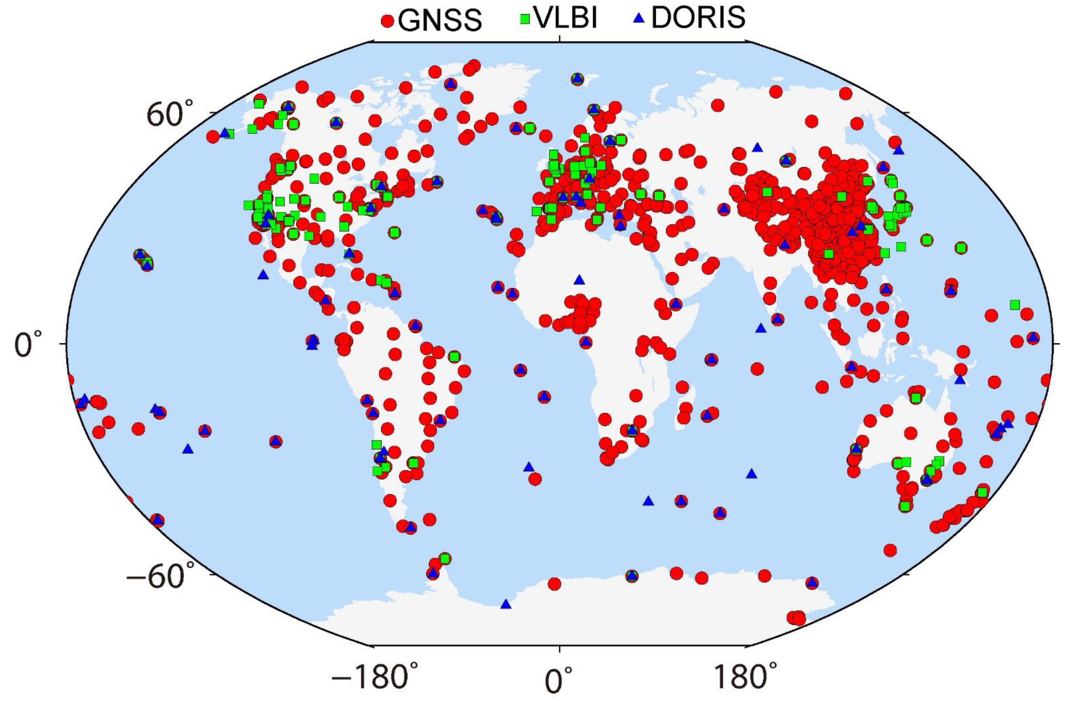
This section determines the WTM model at 1583 space geodetic stations as shown in Figure 1, including 1120 GNSS stations, 256 VLBI stations, and 207 DORIS stations, where the GNSS stations include 697 International GNSS Service (IGS) or European core stations, 269 Crustal Movement Observation Network of China (CMONOC) stations, and 154 National BDS Augmentation Service System (NBASS) stations. The VLBI and DORIS stations are the same as the VMF3 products (https://vmf.geo.tuwien.ac.at (accessed on 19 September 2022)). The WTM model is established through five steps, namely ray-tracing, a-priori coefficient determination, slant path delay modeling, time-variant analysis, and time series fitting.

2.1. Ray-Tracing

In this section, the tropospheric delays and meteorological parameters are calculated with the modified ray-tracing software RADIATE [15,16]. The global ERA5 geopotential, specific humidity and temperature data on 37 pressure levels with 0.25° × 0.25° horizontal resolution were selected for the calculations. The U.S. Standard Atmosphere 1976 (COESA 1976) was used to extend the height converges of the ERA5 reanalysis (about 42 km) to the whole neutral atmosphere (about 84 km) [16]. The ERA5 geopotential and specific humidity data were converted to ellipsoidal height and water vapor pressure according to the equations in Hofmeister [16] and Wallace and Hobbs [17]. The pressure ($P$) and water vapor pressure ($e$) as well as temperature ($T$) in the primary 37 height levels were interpolated to the dense height levels described in Rocken et al. [18] by utilizing the exponential and linear interpolation methods, respectively. The hydrostatic ($n_h$), wet ($n_w$) and total refractive ($n$) indices on the height levels and 0.25° × 0.25° grid points were computed by taking the prepared meteorological parameters as inputs and adopting the following equation as [19]:

$$\left\{\begin{array}{l}{n}_h=1+k_1\frac{P}{T}·{10}^{-6}\\ n_w=1+\left(k_2^{\prime }\frac{e}{T}+k_3\frac{e}{T^2}\right)·{10}^{-6}\\ n=n_h+n_w-1\end{array}\right.$$

(3)

where the $k_1$, $k_2^{\prime }$ and $k_3$ refraction index coefficients take the values of 77.6890 $\mathrm{K}/\mathrm{hPa}$, 22.9742 $\mathrm{K}/\mathrm{hPa}$ and 37.5463 ${\mathrm{K}}^2/\mathrm{hPa}$, respectively [20].

The two-dimensional (2D) Piece-Wise-Linear (2D-PWL) ray-tracing algorithm described by Böhm [21] was used to determine the ray path according to the Snell laws of refraction and the pre-determined refraction index fields and calculate the zenith and slant tropospheric delays by the numerical integration along the zenith direction and ray path as [16]:

$$\left\{\begin{array}{l}ZTD={\displaystyle {\displaystyle \sum }_{i=1}^{k-1}}\left. [\left(n_i^z-1\right)\Delta h_i\right]\\ ZHD={\displaystyle {\displaystyle \sum }_{i=1}^{k-1}}\left. [\left(n_{h,i}^z-1\right)\Delta h_i\right]\\ ZWD={\displaystyle {\displaystyle \sum }_{i=1}^{k-1}}\left. [\left(n_{w,i}^z-1\right)\Delta h_i\right]\\ STD={\displaystyle {\displaystyle \sum }_{i=1}^{k-1}}\left. [\left(n_i-1\right)s_i\right]+g_{bend}\\ SHD={\displaystyle {\displaystyle \sum }_{i=1}^{k-1}}\left. [\left(n_{h,i}-1\right)s_i\right]+g_{bend}\\ SWD={\displaystyle {\displaystyle \sum }_{i=1}^{k-1}}\left. [\left(n_{w,i}-1\right)s_i\right]\\ g_{bend}={\displaystyle {\displaystyle \sum }_{i=1}^{k-1}}\left. [s_i-cos\left({\epsilon }_i-{\epsilon }_k\right)·s_i\right]\end{array}\right.$$

(4)

where $SHD$ and $SWD$ are the Slant Hydrostatic and Wet Delays. $k$ denotes the height level number. $n_i^z$, $n_{h,i}^z$ and $n_{w,i}^z$ stand for the total, hydrostatic and wet refractive index averages between $i$ and $i+1$ height levels in the zenith direction, and $n_i$, $n_{h,i}$ and $n_{w,i}$ represent the corresponding refractive indices along the ray paths. $\mathsf{\Delta }{h}_i$ is the height difference between $i$ and $i+1$ levels, and $s_i$ denotes the ray path length between the two successive height levels. $g_{bend}$ stands for the geometric bend term. ${\epsilon }_i$ is the elevation angle at $i$ height level. ${\epsilon }_k$ represents the final outgoing elevation angle.

The derived meteorological parameters include site-wise pressure ($P_s$), temperature ($T_s$), water vapor pressure ($e_s$) and water vapor weighted mean temperature ($T_m$) where $P_s$, $T_s$ and $e_s$ are retrieved from the pre-determined ERA5 meteorological parameter field by bilinear interpolation and $T_m$ are determined as [14]:

$$T_m=\frac{{{\displaystyle \sum }}_{i=1}^{k-1}\left(e_i/T_i\right)\Delta h_i}{{{\displaystyle \sum }}_{i=1}^{k-1}\left(e_i/T_i^2\right)\Delta h_i}$$

(5)

where $e_i$ and $T_i$ are the water vapor pressure and temperature averages between $i$ and $i+1$ height levels.

The 10-year (2011–2020) monthly mean and 5-year (2016–2020) hourly ERA5 reanalysis data were downloaded from the Copernicus Climate Data Store as the modeling data source of WTM [13]. The tropospheric delays, including $ZHD$, $ZWD$, $SHD$, and $SWD$ as well as the meteorological parameters including $P_s$, $T_s$, $e_s$ and $T_m$ over the 1583 stations shown in Figure 1 were derived by using the prepared ERA5 data and the above-mentioned methods where the SHD and SWD were retrieved at 7 elevation angles (3°, 5°, 7°, 10°, 15°, 30°, and 70°) and 16 azimuths (with an interval of 22.5°).

2.2. A-Priori Coefficient Determination

The determination of mapping function relies on the a-priori $b$ and $c$ coefficients. In this section, we re-determine the a-priori $b$ and $c$ coefficients at specific stations by using the 10-year monthly mean tropospheric delays. The 10-year $a$, $b$ and $c$ coefficients were first calculated by using the rigorous least-squares method [22]. Then the 10-year coefficient time series were fitted as [2]:

$$\begin{array}{c}PAR=A_0+A_1·\cos \left(\frac{\mathrm{doy}}{365.25}2\pi \right)+B_1·\sin \left(\frac{\mathrm{doy}}{365.25}2\pi \right)\\ +A_2·\cos \left(\frac{\mathrm{doy}}{365.25}4\pi \right)+B_2·\sin \left(\frac{\mathrm{doy}}{365.25}4\pi \right)\end{array}$$

(6)

where $PAR$ denotes $a$, $b,$ and $c$ coefficients. $\mathrm{doy}$ represents the day of year. $A_0$ stand for the annual average of the coefficients. $A_1$ and $B_1$ are the annual amplitudes of the coefficients. $A_2$ and $B_2$ are the semi-annual amplitudes. Finally, the a-priori $a$, $b,$ and $c$ coefficient model for the 1583 stations were derived. The mapping function coefficients at JFNG station (B: 30.5156°, L: 114.4910°, H: 71.30 m, Jiufeng, China) are presented in Figure 2 as an example. We can find that the $a_h$, $a_w,$ and $c_h$ coefficients show obvious annual variations.

2.3. Slant Path Delay Modeling

This section carries out the mapping function and horizontal gradient modeling. The 5-year hourly $a$ coefficients at the 1583 stations were first computed by using the 5 year hourly tropospheric delays and the fast method that determines the $a$ coefficient by taking the mapping factor at 3° outgoing elevation angle as input and fixing the b and c coefficients to the pre-determined values as [2,22,23]:

$$a=\frac{1-MF\left({\epsilon }_0\right)·\sin \left({\epsilon }_0\right)}{\frac{MF\left({\epsilon }_0\right)}{\sin \left({\epsilon }_0\right)+\frac{b_0}{\sin \left({\epsilon }_0\right)+c_0}}-\frac{1}{1+\frac{b_0}{1+c_0}}}$$

(7)

where ${\epsilon }_0$ is equal to 3°. $b_0$ and $c_0$ are the pre-determined $b$ and $c$ coefficients.

Then the 5-year horizontal gradients were determined by using the widely-used standard gradient formula as [24,25]:

$$AD\left(\epsilon ,\alpha \right)=\frac{1}{\sin \left(\mathsf{\epsilon }\right)·\tan \left(\epsilon \right)+C}·\left. [G_n\cos \left(\alpha \right)+G_e\sin \left(\alpha \right)\right]$$

(8)

where $AD$ expresses the asymmetric delay. $C$ stands for the gradient constant, and it takes values of 0.0031 and 0.0007 for the hydrostatic and wet asymmetric modeling, respectively [24,25]. Finally, the 5 year hourly mapping function coefficients ($a_h$ and $a_w$) and horizontal gradient ($G_{n_h}$, $G_{e_h}$, $G_{n_w}$ and $G_{e_w}$) for the 1583 stations were determined.

2.4. Time-Variant Analysis

In this section, we systematically analyze the time-variant characteristics of the mapping function coefficients and horizontal gradients for the 1583 stations by taking the 5-year time series as inputs and using the Power Spectral Density (PSD) function [26]. We found that the hydrostatic components ($a_h$, $G_{n_h}$ and $G_{n_e}$) at most stations not only show the prominent annual and semi-annual variations but also include the clear diurnal and semi-diurnal variations. In comparison, the diurnal and semi-diurnal variations of the wet components ($a_w$, $G_{n_w}$ and $G_{n_w}$) are not as significant as the hydrostatic components, and only a few stations show the obvious variations, such as AREG station (B: −16.4654°, L: −71.4929°, H: 2489.30 m, Arequipa, Peru) shown in Figure 3.

2.5. Time Series Fitting

In this section, we fit the 5-year hourly ZPD, mapping function coefficients, and horizontal gradients as well as the meteorological parameters for the 1583 stations by considering the annual, semi-annual, diurnal, and semi-diurnal variations. The fitting formulas are shown as [27]:

$$\{\begin{array}{l}PAR=A_0+{\displaystyle {\displaystyle \sum }_{i=1}^2}\left. [A_i\sin \left(2\pi i\frac{\mathrm{doy}}{365.25}\right)+B_i\cos \left(2\pi i\frac{\mathrm{doy}}{365.25}\right)\right]\\ \hspace{1em}\hspace{1em}\hspace{1em}+{\displaystyle {\displaystyle \sum }_{i=1}^2}\left. [c_i\left(t\right)·\sin \left(2\pi i\frac{\mathrm{hod}}{24}\right)+d_i\left(t\right)·\cos \left(2\pi i\frac{\mathrm{hod}}{24}\right)\right]\\ c_i\left(t\right)=C_i^0+C_i^1\sin \left(2\pi \frac{\mathrm{doy}}{365.25}\right)+C_i^2\cos \left(2\pi \frac{\mathrm{doy}}{365.25}\right)\\ \hspace{1em}\hspace{1em}\hspace{1em}+C_i^3\sin \left(4\pi \frac{\mathrm{doy}}{365.25}\right)+C_i^4\cos \left(4\pi \frac{\mathrm{doy}}{365.25}\right)\left(i=1,2\right)\\ d_i\left(t\right)=D_i^0+D_i^1\sin \left(2\pi \frac{\mathrm{doy}}{365.25}\right)+D_i^2\cos \left(2\pi \frac{\mathrm{doy}}{365.25}\right)\\ \hspace{1em}\hspace{1em}\hspace{1em}+D_i^3\sin \left(4\pi \frac{\mathrm{doy}}{365.25}\right)+D_i^4\cos \left(4\pi \frac{\mathrm{doy}}{365.25}\right)\left(i=1,2\right)\end{array}$$

(9)

where PAR represents the mapping function coefficients, $ZPD$, horizontal gradients, and meteorological parameters. $c_1\left(t\right)$, $d_1\left(t\right)$, $c_2\left(t\right)$ and $d_2\left(t\right)$ stand for the time-dependent coefficients for the diurnal and semi-diurnal variations, expressed by the second and third formulas. $\mathrm{hod}$ denotes hour of day (UTC). $C_i^0$ is the annual average of $c_i\left(t\right)$. $C_i^1$, $C_i^2$, $C_i^3$ and $C_i^4$ are the coefficients for the annual and semi-annual variations of $c_i\left(t\right)$. $D_i^0$ is the annual average of $d_i\left(t\right)$. $D_i^1$, $D_i^2$, $D_i^3$ and $D_i^4$ are the coefficients for the annual and semi-annual variations of $d_i\left(t\right)$. In total, there are 25 coefficients included.

We used the fitting formulas to model the 5-year hourly parameter time series, deriving the site-wise WTM model for the 1583 station, and compared the signatures of the WTM model with the latest GPT3 model in

Table 1. Signatures of the GPT3 model and the newly established WTM model.

Item	GPT3	WTM
Model Type	Grid-wise (1° × 1°)	Site-wise
Data source	1° × 1° monthly mean ERAI from 2001 to 2010	0.25° × 0.25° monthly mean ERA5 from 2011 to 2020 as well as hourly ERA5 from 2016 to 2020
Time variation	Annual and semi-annual variations	Annual and semi-annual as well as diurnal and semi-diurnal variations
Space coverage	Global coverage	1583 global distributed GNSS, VLBI and DORIS stations
Input parameters	Modified Julian date ($mjd$) Geographic latitude ($\phi$, unit: rad) Geographic longitude ($\lambda$, unit: rad) Ellipsoidal height ($h_{ell}$)	Station name Modified Julian date ($mjd$) UTC hour of day $(hod$)
Output parameters	mapping function coefficients ($a_h$ and $a_w$) Horizontal gradient ($G_{n_h}$$,G_{e_h}$$,G_{n_w}$$\mathrm{and}{G}_{e_w}$, unit: m) Pressure ($P$, unit: $\mathrm{hPa}$) Temperature ($T$, unit: $°\mathrm{C}$) Temperature lapse rate ($dT$, unit $:\mathrm{K}/\mathrm{km}$) water vapor weighted mean temperature ($T_m$, unit: $\mathrm{K}$) Water vapor pressure ($e$, unit: $\mathrm{hPa}$) Water vapor decrease factorGeoid undulation ($N$, unit: m)	Zenith hydrostatic delay ($ZHD$, unit: m) Zenith wet delay ($ZWD$, unit: m) mapping function coefficients ($a_h$ and $a_w$) Horizontal gradient ($G_{n_h}$$,G_{e_h}$$,G_{n_w}$$\mathrm{and}{G}_{e_w}$, unit: mm) Pressure ($P$, unit: $\mathrm{hPa}$) Temperature ($T$, unit: $°\mathrm{C}$) water vapor weighted mean temperature ($T_m$, unit: $\mathrm{K}$) Water vapor pressure ($e$, unit: $\mathrm{hPa}$)
A-priori $b$ and $c$ coefficients	12-order spherical harmonic function with considering annual and semi-annual variations	Site-wise presentation with considering annual and semi-annual variations

[2]. We can find the better modeling data source and temporal-spatial expression of the WTM model with respect to the GPT3 model, which may improve the model performance.

To present the superiority of the WTM model clearly, we further took the AREG station as an example and showed its calculated time series as well as the modeled time series with Equations (9) and (6) in Figure 4. We can find that the better performance benefited from the additional consideration of diurnal and semi-diurnal variations, especially for the hydrostatic horizontal gradient parameters ($G_{n_h}$ and $G_{n_e}$).

3. Evaluation of WTM

3.1. Evaluation Strategies

The ZPD and meteorological parameter modeling and evaluation based on the ERA5 reanalysis data have been well presented in the existing literature, such as Li et al. [27] and Mateus et al. [28]. Therefore, this section only evaluates the accuracy of the mapping function and horizontal gradient from the established WTM model and compares them with the latest GPT3 model. The references are the symmetric and asymmetric delays calculated from the 0.25° × 0.25° ERA5 data. The time period is the whole year of 2020, including 8784 epochs (hours during the year 2020). The globally distributed 524 stations, as shown in Figure 5, were selected for the model evaluation. The precision index is Mean Absolute Error (MAE) [1,2,3,29], which can be calculated as:

$$\left\{\begin{array}{l}\left. [\begin{array}{c}MA{E}_{GPT3}^{MF}\left(\epsilon \right)\\ MA{E}_{WTM}^{MF}\left(\epsilon \right)\end{array}\right]=\left|\left. [\begin{array}{c}M{F}_{GPT3}^h\left(\epsilon \right)\\ M{F}_{WTM}^h\left(\epsilon \right)\end{array}\right]·ZH{D}_{ERA5}+\left. [\begin{array}{c}M{F}_{GPT3}^w\left(\epsilon \right)\\ M{F}_{WTM}^w\left(\epsilon \right)\end{array}\right]·ZW{D}_{ERA5}-ST{D}_{ERA5}\left(\epsilon \right)\right|\\ \left. [\begin{array}{c}MA{E}_{GPT3}^{HG}\left(\epsilon ,\alpha \right)\\ MA{E}_{WTM}^{HG}\left(\epsilon ,\alpha \right)\end{array}\right]=\left|\left. [\begin{array}{c}A{D}_{GPT3}^h\left(\epsilon ,\alpha \right)\\ A{D}_{WTM}^h\left(\epsilon ,\alpha \right)\end{array}\right]+\left. [\begin{array}{c}A{D}_{GPT3}^w\left(\epsilon ,\alpha \right)\\ A{D}_{WTM}^w\left(\epsilon ,\alpha \right)\end{array}\right]-A{D}_{ERA5}\left(\epsilon ,\alpha \right)\right|\end{array}\right.$$

(10)

where $MA{E}^{MF}$ and $MA{E}^{HG}$ are the MAEs for mapping function and horizontal gradient, respectively. $ZH{D}_{ERA5}$, $ZW{D}_{ERA5}$, $ST{D}_{ERA5},$ and $A{D}_{ERA5}$ denote the $ZHD$, $ZWD$, symmetric $STD$ and $AD$ retrieved from the hourly ERA5 data. The evaluations are carried out at seven elevation angles (3°, 5°, 7°, 10°, 15°, 30°, and 70°) and 16 azimuths (with interval of 22.5°).

3.2. Model Accuracy Analysis

The MAEs at 16 azimuths and 524 stations in 2020 were averaged at different elevation angles and shown in

Table 2. Model MAE (mm) at different elevation angles.

Components	Models	e = 3°	e = 5°	e = 7°	e = 10°	e = 15°	e = 30°	e = 70°
MF	GPT3	60.64	21.57	10.06	4.11	1.36	0.19	0.03
	WTM	58.34	20.68	9.39	3.77	1.27	0.18	0.03
HG	GPT3	74.66	35.66	20.35	10.73	4.99	1.25	0.15
	WTM	72.99	34.75	19.81	10.44	4.85	1.22	0.15

. We can find that the mapping functions of the WTM model show overall improvements to the GPT3 model, especially at low elevation angles. At 3° and 5° elevation angles, the MAE improvements reach 2.30 and 0.89 mm, respectively. The horizontal gradient improvements also show similar elevation angle dependence where at 3° and 5° elevation angles, the WTM model improvements are 1.67 and 0.91 mm.

In addition to the statistical MAEs, the 5° elevation angle MAE distribution for the 524 stations as well as the global topography are shown in Figure 6, considering the mapping function modeling at 3° elevation angle (Section 2.3). We find that the mapping function MAE distribution for the WTM model generally surpasses the distribution for the GPT3 model, while the improvements are hardly distinguished, except for the stations located in the western part of South America (Figure 6a,b). As a consequence, we further presented the MAE difference distribution between the two mapping functions as well as its histogram in Figure 6c,d. At this point, the MAE differences are clearly presented, and about 78.4% of the stations show the MAE improvements benefitted from the WTM model, with the maximal improvements of 12.8 mm (UNSA station). In contrast to the mapping function MAE distribution, the horizontal gradient MAE distribution shows obvious latitude dependence, and the stations with middle and low latitudes generally have larger MAEs. The horizontal gradient MAE distribution for the WTM model is also superior to the GPT3 model (Figure 6e,f), and the MAE difference distribution can show the superiority more clearly (Figure 6g,h). About 91.4% of stations are profited by the WTM model, and the maximal improvement reaches 14.71 mm (UNSA station).

The UNSA station (B: −24.7274°, L: −65.4076°, H: 1257.80 m, Salta, Argentina) shows the largest MAE improvements both for the mapping function and horizontal gradients, and therefore the MAE time series as well as the surrounding terrain of the UNSA station are further shown in Figure 7. We can find significant improvements in most epochs, both for mapping function and horizontal gradient (Figure 7a,b). The main reason is that the UNSA station is located in an area with large terrain relief (Figure 7c) where the parameter spatial interpolation calculation from the 1° × 1° GPT3 model will introduce a significant loss of accuracy. However, the WTM model is directly modeled at the station location and therefore is free of interpolation and no loss of accuracy.

4. Validation of WTM in BDS PPP

4.1. Data Processing Strategies

In this section, we validate the GPT3 and WTM models by two BDS PPP schemes, namely, using the GPT3 and WTM models, respectively, considering the newly available Full Operational Capability (FOC) of the BDS constellation. The BDS (BDS2 + BDS3) data from 31 globally distributed IGS Multi-GNSS Experiment (MGEX) stations [30] spanning the whole year of 2020 was selected for validation by Positioning And Navigation Data Analyst (PANDA) software [31], and the station distribution was shown in Figure 5. The satellite orbits and clock are fixed to the 5 min GBM products, and the data processing strategies are shown in

Table 3. Data processing strategies for BDS PPP.

Observation
Sampling interval	300 s
Frequency combination	Ionosphere-free combination of B1I and B3I
Elevation cutoff angle	3°
Elevation weighting strategy	$\left\{\begin{array}{l}p=2sin\epsilon , \left(\epsilon \le 30°\right)\\ p=1, (\epsilon >30°)\end{array}\right.$
Error correction
Phase center variations	igs14.atx
Higher-order ionospheric delay	GIM and IGRF13 (Fritsche et al. [32])
Ocean tide loading	FES2014b
A priori tropospheric delay	Scheme 1: ZHD (GPT3 + Saastamoinen [33]); ZWD (GPT3+Askne and Nordius [34]); mapping function (GPT3) Scheme 2: ZHD (WTM); ZWD (WTM); mapping function (WTM)
Parameter estimation
Satellite orbits and clock corrections	Fixed from GBM 5 min products
Mapping function	Scheme 1: Wet GPT3 Scheme 2: Wet WTM
ZWD stochastic model	Piece-wise constant (1 h), random walk between segments $(15 \mathrm{mm}/\sqrt{\mathrm{h}})$
Gradient mapping function	$m{f}_w·\cot \left(e\right)$ (MacMillan [35])
Gradient stochastic model	Piece-wise constant (2 h), random walk between segments $(10 \mathrm{mm}/\sqrt{\mathrm{h}})$
Station coordinates	Daily constant
Receiver clock corrections	White noise
Ambiguities	Fixed

.

4.2. Coordinate Repeatability Analysis

In this section, we compare the coordinate repeatability of the two PPP schemes. The coordinate time series in 2020 for the 31 stations were first extracted from the daily PPP solutions. Then the gross error, phase step terms, periodic terms, and linear trend terms were removed from the time series by using the Hector software [36], deriving the North (N), East (E), and Vertical (U) coordinate residual time series. Finally, the standard deviation of the coordinate residual time series, namely the coordinate repeatability, was calculated and shown in

Table 4. Coordinate repeatability (mm) of the two PPP schemes.

Models	N	E	U
GPT3	2.12	3.28	7.72
WTM	2.12	3.29	7.73

. We can find that the two PPP schemes almost show identical coordinate repeatability. The main reason is that the impacts of different models on PPP estimation are greatly reduced by the elevation weighting strategy and the estimation of the residual Zenith Total Delay (ZTD) parameter [1]. In addition, other error sources, such as multi-path effects and phase center variations, will also suppress the impacts.

In addition to the statistical coordinate repeatability, the distribution of the U coordinate repeatability difference between the two PPP schemes and its histogram are also presented in Figure 8. We can find the insignificant coordinate repeatability differences with a maximal difference of 0.60 mm, again indicating the negligible impacts of different empirical models on the coordinate repeatability.

4.3. Coordinate and ZTD Difference Analysis

The coordinate repeatability generally reflects the standard deviation of the coordinate time series, but cannot represent the coordinate differences. Therefore, in this section, we directly compare the coordinate and ZTD time series estimated from the two PPP schemes and list the statistical U coordinate and ZTD difference bias and Root Mean Square (RMS) in

Table 5. Coordinate and ZTD differences (mm) between the two PPP schemes.

Components	WTM-GPT3
	Min		Max		Mean
	Bias	RMS	Bias	RMS	Bias	RMS
U	−1.78	0.79	1.39	2.95	−0.64	1.36
ZTD	−0.43	0.31	0.87	1.03	0.36	0.67

. We can find the significant U coordinate and ZTD difference biases and RMSs, with maximal biases of −1.78 and 0.87 mm and maximal RMSs of 2.95 and 1.03 mm, indicating the systematic bias and significant difference between the two schemes.

In addition, the U coordinate and ZTD difference bias distribution is also shown in Figure 9. We can find the generally negative and positive biases for the U coordinate and ZTD, respectively, verifying the significant systematic biases between the two PPP schemes and the strong correlation between vertical coordinate and ZTD [37].

Among all the stations, the MAS1 station (B: 27.7637°, L: −15.6333°, H: 197.30 m, Maspalomas, Spain) located in the northwest of Africa shows the largest U coordinate and ZTD biases of −1.78 and 0.87 mm. Therefore, we further present the U coordinate and ZTD difference time series as well as the surrounding terrain distribution of the MAS1 station in Figure 10. We can find the consistently negative and positive biases for the U coordinate and ZTD (Figure 10a,b), respectively, indicating the significantly systematic biases between the two PPP schemes. The main reason is that the MAS1 station is located on a small island (Figure 10c) where the parameter spatial interpolation calculation from the 1° × 1° GPT3 model will cause a significant accuracy loss. Whereas the WTM model is a site-wise empirical model and is interpolation free with no accuracy loss in its usage.

5. Conclusions

Tropospheric delay has significant impacts on space geodetic techniques such as GNSS, VLBI, and DORIS, and is regularly corrected with the tropospheric models, including ZPD, mapping function, and horizontal models. In the past decades, the tropospheric models have been continuously improved on the modeling data source and temporal-spatial resolution, deriving the latest GPT3 model. However, the GPT3 model is still with the limited horizontal resolution of 1° × 1° and ignores the potential diurnal variations, and therefore poorly performs in regions with complex terrain and loses the capability of catching the diurnal variations of the Earth’s atmosphere that may contaminate the high-precision space geodetic data processing and applications, such as earth reference frame realization, crustal deformation monitoring and earth climate and weather change monitoring.

In this paper, we utilized the high temporal-spatial resolution advantages of the newly released ERA5 reanalysis data and initiatively established the comprehensively site-wise WTM model where the ZPD, mapping function, and horizontal gradient as well as meteorological parameters at 1583 globally distributed space geodetic stations are involved with additionally considering the diurnal and semi-diurnal variations. Different from the GPT3 model, the WTM model directly models at the station location and considers the diurnal variations, and therefore can avoid the accuracy loss from spatial interpolation and the insufficient consideration of the atmospheric variations that essentially contribute to the better model accuracy and BDS PPP performance of the WTM model, especially for the stations with terrain relief.

Besides the site-wise empirical model involved in this work, the site-wise discrete mapping function and horizontal gradient products from the reanalysis, operational, and forecast numerical weather models (https://vmf.geo.tuwien.ac.at/ (accessed on 19 September 2022)) are also very important to improving the performance of space geodetic techniques. However, the product time resolution is limited to the resolution of the numerical weather model of 6 h that may restrict the product usage under extreme weather scenarios and contaminate the retrieval of diurnal geophysical signals by using space geodetic techniques. By using the high time resolution advantage of the ERA5 reanalysis data and the GNSS tropospheric product, the site-wise discrete product can be further refined as for the time resolution.

References

- Landskron, D. Modeling Tropospheric Delays for Space Geodetic Techniques. Ph.D. Thesis, Department of Geodesy and Geoinformation, TU Wien, Wien, Austria, 2017. Available online: http://repositum.tuwien.ac.at/obvutwhs/content/titleinfo/2099559 (accessed on 13 September 2022).
- Landskron, D.; Böhm, J. VMF3/GPT3: Refined discrete and empirical troposphere mapping functions. J. Geod. 2018, 92, 349–360. [Google Scholar] [CrossRef] [PubMed]
- Landskron, D.; Böhm, J. Refined discrete and empirical horizontal gradients in VLBI analysis. J. Geod. 2018, 92, 1387–1399. [Google Scholar] [CrossRef] [PubMed] [Green Version]
- Marini, J.W. Correction of satellite tracking data for an arbitrary tropospheric profile. Radio Sci. 1972, 7, 223–231. [Google Scholar] [CrossRef]
- Herring, T.A. Modeling atmospheric delays in the analysis of space geodetic data. In Proceedings of the Refraction of Transatmospheric Signals in Geodesy, The Hague, The Netherlands, 19–22 May 1992; Netherlands Geodetic Commission Publications in Geodesy: Delft, The Netherlands, 1992; Volume 36, pp. 157–164. [Google Scholar]
- Niell, A.E. Global mapping functions for the atmosphere delay at radio wavelengths. J. Geophys. Res. Solid Earth 1996, 101, 3227–3246. [Google Scholar] [CrossRef]
- Böhm, J.; Werl, B.; Schuh, H. Troposphere mapping functions for GPS and very long baseline interferometry from European Centre for Medium-Range Weather Forecasts operational analysis data. J. Geophys. Res. Solid Earth 2006, 111, 1–9. [Google Scholar] [CrossRef]
- Böhm, J.; Niell, A.; Tregoning, P.; Schuh, H. Global Mapping Function (GMF): A new empirical mapping function based on numerical weather model data. Geophys. Res. Lett. 2006, 33, 1–4. [Google Scholar] [CrossRef] [Green Version]
- Lagler, K.; Schindelegger, M.; Böhm, J.; Krásná, H.; Nilsson, T. GPT2: Empirical slant delay model for radio space geodetic techniques. Geophys. Res. Lett. 2013, 40, 1069–1073. [Google Scholar] [CrossRef] [Green Version]
- Böhm, J.; Möller, G.; Schindelegger, M.; Pain, G.; Weber, R. Development of an improved empirical model for slant delays in the troposphere (GPT2w). GPS Solut. 2015, 19, 433–441. [Google Scholar] [CrossRef] [Green Version]
- MacMillan, D.S.; Ma, C. Atmospheric gradients and the VLBI terrestrial and celestial reference frames. Geophys. Res. Lett. 1997, 24, 453–456. [Google Scholar] [CrossRef]
- Böhm, J.; Urquhart, L.; Steigenberger, P.; Heinkelmann, R.; Nafisi, V.; Schuh, H. A priori gradients in the analysis of space geodetic observations. In Reference Frames for Applications in Geosciences; Springer: Berlin/Heidelberg, Germany, 2013; pp. 105–109. [Google Scholar] [CrossRef]
- Hersbach, H.; Bell, B.; Berrisford, P. The ERA5 global reanalysis. Q. J. R. Meteor. Soc. 2020, 146, 1999–2049. [Google Scholar] [CrossRef]
- Zhang, W.; Zhang, H.; Liang, H.; Lou, Y.; Cai, Y.; Cao, Y.; Zhou, Y.; Liu, W. On the suitability of ERA5 in hourly GPS precipitable water vapor retrieval over China. J. Geod. 2019, 93, 1897–1909. [Google Scholar] [CrossRef]
- Zhou, Y.; Lou, Y.; Zhang, W.; Kuang, C.; Liu, W.; Bai, J. Improved performance of ERA5 in global tropospheric delay retrieval. J. Geod. 2020, 94, 103. [Google Scholar] [CrossRef]
- Hofmeister, A. Determination of Path Delays in the Atmosphere for Geodetic VLBI by Means of Ray-Tracing. Ph.D. Thesis, Department of Geodesy and Geoinformation, TU Wien, Wien, Austria, 2016. Available online: http://resolver.obvsg.at/urn:nbn:at:at-ubtuw:1-3444 (accessed on 13 September 2022).
- Wallace, J.M.; Hobbs, P.V. Atmospheric Thermodynamics//Atmospheric Science; Elsevier: Amsterdam, The Netherlands, 2006; pp. 63–111. [Google Scholar]
- Rocken, C.; Sokolovskiy, S.; Johnson, J.M.; Hunt, D. Improved mapping of tropospheric delays. J. Atmos. Ocean. Technol. 2001, 18, 1205–1213. [Google Scholar] [CrossRef]
- Nilsson, T.; Böhm, J.; Wijaya, D.D.; Tresch, A.; Nafisi, V.; Schuh, H. Path delays in the neutral atmosphere. In Atmospheric Effects in Space Geodesy; Böhm, J., Schuh, H., Eds.; Springer Atmospheric Sciences; Springer: Berlin, Germany, 2013; pp. 73–136. ISBN 9783642369315. [Google Scholar] [CrossRef]
- Rüeger, J.M. Refractive index formulae for radio waves. In Proceedings of the FIG XXII International Congress (FIG), Washington, DC, USA, 19–26 April 2002; Available online: https://www.fig.net/resources/proceedings/fig_proceedings/fig_2002/Js28/JS28_rueger.pdf (accessed on 13 September 2022).
- Böhm, J. Troposphärische Laufzeitverzögerungen in der VLBI. Ph.D. Thesis, Institut für Geodäsie und Geophysik, TU Wien, Wien, Austria, 2004. Available online: https://publik.tuwien.ac.at/files/PubDat_119666.pdf (accessed on 13 September 2022).
- Böhm, J.; Schuh, H. Vienna mapping functions in VLBI analyses. Geophys. Res. Lett. 2004, 31, 1–4. [Google Scholar] [CrossRef]
- Zhou, Y.; Lou, Y.; Zhang, W.; Bai, J.; Zhang, Z. An improved tropospheric mapping function modeling method for space geodetic techniques. J. Geod. 2021, 95, 98. [Google Scholar] [CrossRef]
- Chen, G.; Herring, T. Effects of atmospheric azimuthal asymmetry on the analysis of space geodetic data. J. Geophys. Res. Solid Earth 1997, 102, 20489–20502. [Google Scholar] [CrossRef]
- Zhou, Y.; Lou, Y.; Zhang, W.; Wu, P.; Bai, J.; Zhang, Z. Tropospheric Second-Order Horizontal Gradient Modeling for GNSS PPP. Remote Sens. 2022, 14, 4807. [Google Scholar] [CrossRef]
- Zhang, W.; Lou, Y.; Huang, J.; Liu, W. A refined regional empirical pressure and temperature model over China. Adv. Space Res. 2018, 62, 1065–1074. [Google Scholar] [CrossRef]
- Li, T.; Wang, L.; Chen, R.; Fu, W.; Xu, B.; Jiang, P.; Liu, J.; Zhou, H.; Han, Y. Refining the empirical global pressure and temperature model with the ERA5 reanalysis and radiosonde data. J. Geod. 2021, 95, 31. [Google Scholar] [CrossRef]
- Mateus, P.; Mendes, V.B.; Plecha, S.M. HGPT2: An ERA5-based global model to estimate relative humidity. Remote Sens. 2021, 13, 2179. [Google Scholar] [CrossRef]
- Urquhart, L.; Nievinski, F.G.; Santos, M.C. Assessment of troposphere mapping functions using three-dimensional ray-tracing. GPS Solut. 2014, 18, 345–354. [Google Scholar] [CrossRef]
- Montenbruck, O.; Steigenberger, P.; Prange, L.; Deng, Z.; Zhao, Q.; Perosanz, F.; Romero, I.; Noll, C.; Stürze, A.; Weber, G.; et al. The Multi-GNSS Experiment (MGEX) of the International GNSS Service (IGS)–Achievements, prospects and challenges. Adv. Space Res. 2017, 59, 1671–1697. [Google Scholar] [CrossRef]
- Shi, C.; Zhao, Q.; Geng, J.; Lou, Y.; Ge, M.; Liu, J. Recent development of PANDA software in GNSS data processing. In Proceedings of the International Conference on Earth Observation Data Processing and Analysis (ICEODPA), Wuhan, China, 28–30 December 2008; International Society for Optics and Photonics. SPIE: Bellingham, DC, USA, 2008; Volume 7285, p. 72851S. [Google Scholar] [CrossRef]
- Fritsche, M.; Dietrich, R.; Knöfel, C.; Rülke, A.; Vey, S.; Rothacher, M.; Steigenberger, P. Impact of higher-order ionospheric terms on GPS estimates. Geophys. Res. Lett. 2005, 32, 1–5. [Google Scholar] [CrossRef]
- Saastamoinen, J. Atmospheric correction for the troposphere and stratosphere in radio ranging satellites. Use Artif. Satell. Geod. 1972, 15, 247–251. [Google Scholar]
- Askne, J.; Nordius, H. Estimation of tropospheric delay for microwaves from surface weather data. Radio Sci. 1987, 22, 379–386. [Google Scholar] [CrossRef]
- MacMillan, D.S. Atmospheric gradients from very long baseline interferometry observations. Geophys. Res. Lett. 1995, 22, 1041–1044. [Google Scholar] [CrossRef]
- Bos, M.S.; Fernandes, R.M.S.; Williams, S.D.P.; Bastos, L. Fast error analysis of continuous GNSS observations with missing data. J. Geod. 2013, 87, 351–360. [Google Scholar] [CrossRef] [Green Version]
- Tregoning, P.; Dam, T.V. Atmospheric pressure loading corrections applied to GPS data at the observation level. Geophys. Res. Lett. 2005, 32, 1–4. [Google Scholar] [CrossRef]
Figure 1.
Distribution of GNSS (red circles), VLBI (green squares) and DORIS (blue triangles) stations included in WTM model.
Figure 2.
Calculated (black line) and modeled (red line) mapping function coefficients at JFNG station.
Figure 3.
Variation characteristics for the mapping function coefficients and horizontal gradients at the AREG station. The four dash lines from left to right mark the semi-diurnal, diurnal, semi-annual, and annual periods, respectively.
Figure 4.
Calculated time series (black line) as well as modeled time series with Equations (9) (red line) and (6) (green line) for the AREG station. The left two columns show the 5-year time series, and the right two columns are the 10-day zoom in time series.
Figure 5.
Distribution of the selected model evaluation (blue circles) and positioning validation (red squares) stations.
Figure 6.
Distribution for the 5° elevation angle MAE and global topography. (a,b) are the MAE distributions for the mapping functions from the GPT3 and WTM models. (c) denotes the MAE difference distributions between (a) and (b). (d) shows the histogram of (c). (e,f) are the MAE distribution for the horizontal gradients from the GPT3 and WTM models. (g) is the MAE difference distribution between (e) and (f). (h) represents the histogram of (g). (i) shows the global topography distribution.
Figure 7.
Mapping function (a) and horizontal gradient (b) MAE time series as well as surrounding topography (c) of the UNSA station. The red triangle represents the station location. The blue grid denotes the 1° × 1° grid of the GPT3 model.
Figure 8.
Distribution (a) and histogram (b) of the coordinate repeatability difference between the two PPP schemes.
Figure 9.
Bias distribution for U coordinate (a) and ZTD (b) between the two PPP schemes.
Figure 10.
U coordinate (a) and ZTD (b) difference time series and surrounding topography (c) of the MAS1 station. The black lines represent the original time series. The red lines denote the weekly smoothed time series. The red triangle shows the station location. The blue grid stands for the 1° × 1° grid of the GPT3 model.