Article

Study of the Spatiotemporal Variability of Oceanographic Parameters and Their Relationship to Holothuria Species Abundance in a Marine Protected Area of the Mediterranean Using Satellite Imagery

by
Panteleimon Christou
,
Christos Domenikiotis
*,
Nikos Neofitou
and
Dimitris Vafidis
Department of Ichthyology and Aquatic Environment, School of Agricultural Sciences, University of Thessaly, Fytokou Street, 384 45 Volos, Greece
*
Author to whom correspondence should be addressed.
Remote Sens. 2022, 14(23), 5946; https://doi.org/10.3390/rs14235946
Submission received: 10 October 2022 / Revised: 11 November 2022 / Accepted: 18 November 2022 / Published: 24 November 2022
(This article belongs to the Special Issue Remote Sensing for Water Environment Monitoring)

Abstract

:
Marine protected areas (MPAs) are designated to protect marine ecosystems and, among other things, to monitor climate variability, which in turn affects aquatic species. The aim of this study is to examine the contribution of remotely sensed data as an indication of Holothuria abundance, by investigating the spatiotemporal variability of physicochemical parameters. The study area is in the National Marine Park of Alonissos Northern Sporades, which is included in the NATURA 2000 network. Firstly, the abundance of Holothuria species was measured by scuba diving. At the same time, depth profiles of five physicochemical parameters (temperature, salinity, pH, dissolved oxygen and Chl-a) were recorded by CTD (conductivity, temperature, depth), a primary instrument used to determine the essential physical and chemicals properties of seawater column profiles in the coastal zone. The physicochemical variables examined are the most common environmental parameters with the highest impact on growth, reproduction, productivity and survival rate of sea cucumber species, affecting the availability of food sources. Analysis of this data allows us to identify parameters which are essential for their existence. The analysis showed that only temperature and Chlorophyll-a (Chl-a) could be useful for identifying the abundance. These two parameters are readily available from satellite data. Additionally, particulate organic carbon (POC) is essential for Holothuria’s existence. Consequently, a time series of satellite data products from Terra/MODIS sensor were utilized from 2000 to 2020 for sea surface temperature (SST), Chl-a and POC. The monthly temporal trend shows that the abundance could be justified in areas where the Holothuria presence has been established. Monthly spatiotemporal analysis shows that SST, Chl-a and POC availability, could be an indication of the differences in abundance recorded.

1. Introduction

According to the definition given by the International Union for Conservation of Nature (IUCN), as a protected area is defined “a recognized and clearly defined geographical area for where a conservation commitment exists and managed through legal or other effective means, in order to achieve long-term conservation and nature protection, with its related ecosystem services and cultural values” [1]. They are the cornerstone of biodiversity conservation, an essential tool for safeguarding biodiversity from natural disasters, providing global food security and maintaining water quality. The global network of protected areas is estimated to store at least 15% of the global terrestrial carbon, pointing out its significance in relation to climate change [2]. This definition also applies to marine protected areas (MPAs).
Apart from the geographical cover, an MPA includes the airspace above the sea surface, the sea surface itself, its overlying water column, depth and subsoil, flora, fauna, and historical and cultural features of all the enclosed environment. In other words, MPA “is defined as an area designated and effectively managed to protect marine ecosystems”, which contributes to the replenishment of natural resources and to social, economic and cultural enrichment. They are categorized according to the management objectives by the IUCN. The MPAs are recognized by many national governments and organizations as the global standard for biodiversity protection, gradually being incorporated into government legislation [3]. MPAs with the highest level of protection increase the whole fish biomass from 343% to 670% [4]. In this way, an MPA is a well-protected area with no exogenous factors, which makes it an ideal place for study.
The observation and monitoring of the earth from space has today become a very important tool for the study of the natural environment and understanding the complexity of the earth ecosystem. The information gathered by the satellites on a regular basis is of benefit to the study of environmental conditions affecting marine biodiversity. The utilization of this information finds application in various scientific fields, such as oceanography, by monitoring parameters such as POC [5], sea surface temperature [6,7,8] (for understanding the climate change and predicting climate variations), chlorophyll concentration (due to its importance to photosynthesis process) [9,10] and provides better emergency management and disaster recovery. Furthermore, satellite remote sensing contributes to the detection of mechanisms of spatiotemporal variations of POC [11] and adverse environmental phenomena such as eutrophication which plays a key role in environmental biology and the carbon cycle balance [12,13,14,15,16,17].
Marine environment and aquatic biodiversity are threatened by a variety of anthropogenic stressors and human activities such as petroleum oil spills, which can be monitored using satellite remote sensing [18,19,20,21], deteriorating the negative impact on marine species and wildlife. As the biodiversity and the balance of marine ecosystems are threatened by human activities [22,23], satellite monitoring of the coastal front provides valuable information on the structure of pelagic bio-communities, improving their relationship with human societies.
Holothuria (sea cucumber) is an ecological important benthic species, as they are bioindicators of pollution in marine environments due to their ability to collect sediment particles and organic matter [24,25,26]. They are considered to be among the best bioturbators and deposit feeders. Although it is very difficult to gather enough information about the benthic systems through satellite data only, it can still assist the examination of the environmental conditions in a marine environment, which in turn could affect the benthic organisms.
This work is based on the in-situ measurements in a MPA to define the key factors affecting the abundance of Holothurians. Furthermore, it examines the spatial variability of sea surface temperature (SST), Chl-a and particulate organic carbon (POC) based on satellite data for a time span of twenty years and explores how they could be connected to the abundance of Holothuria.

2. Materials and Methods
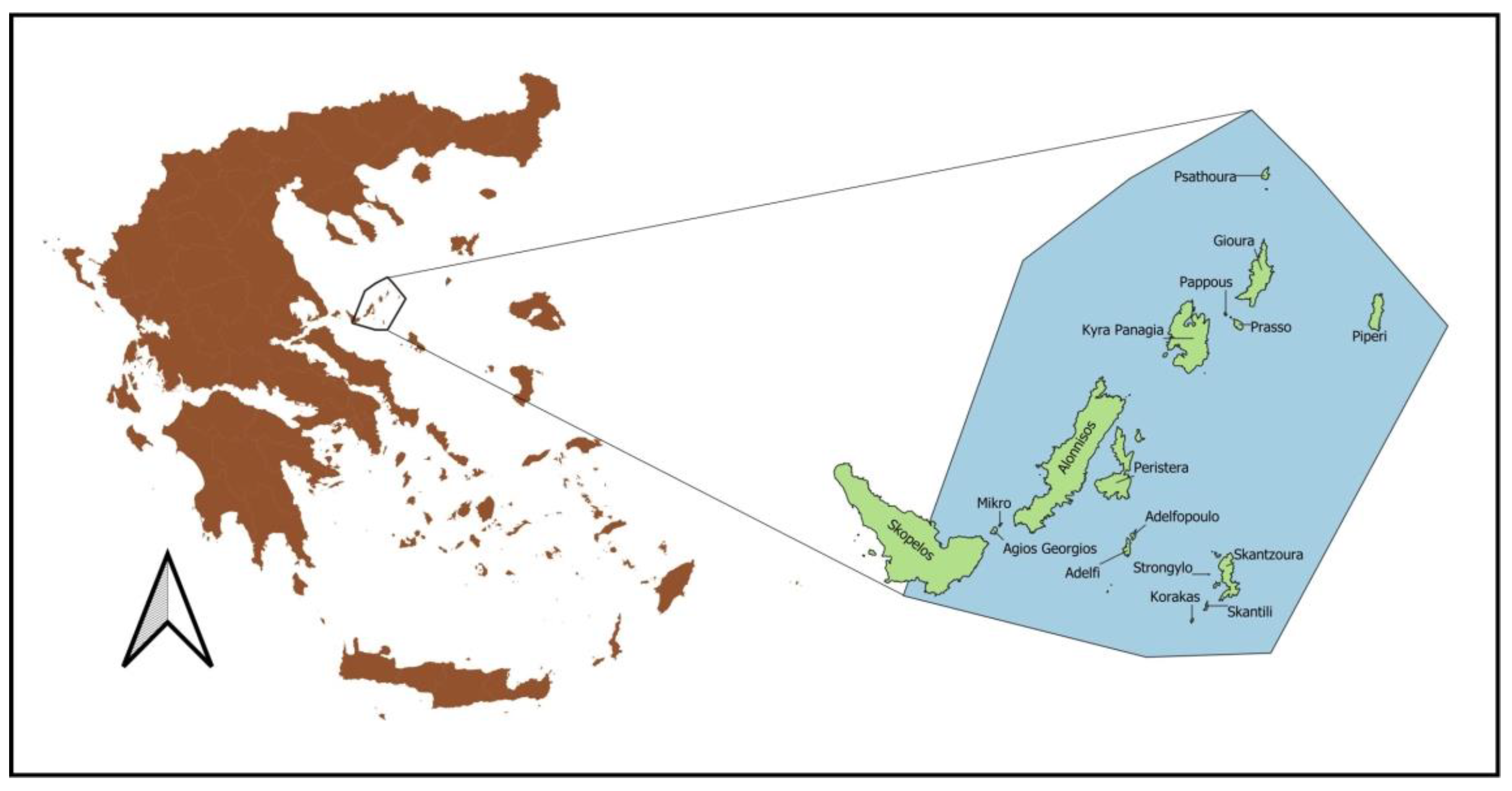
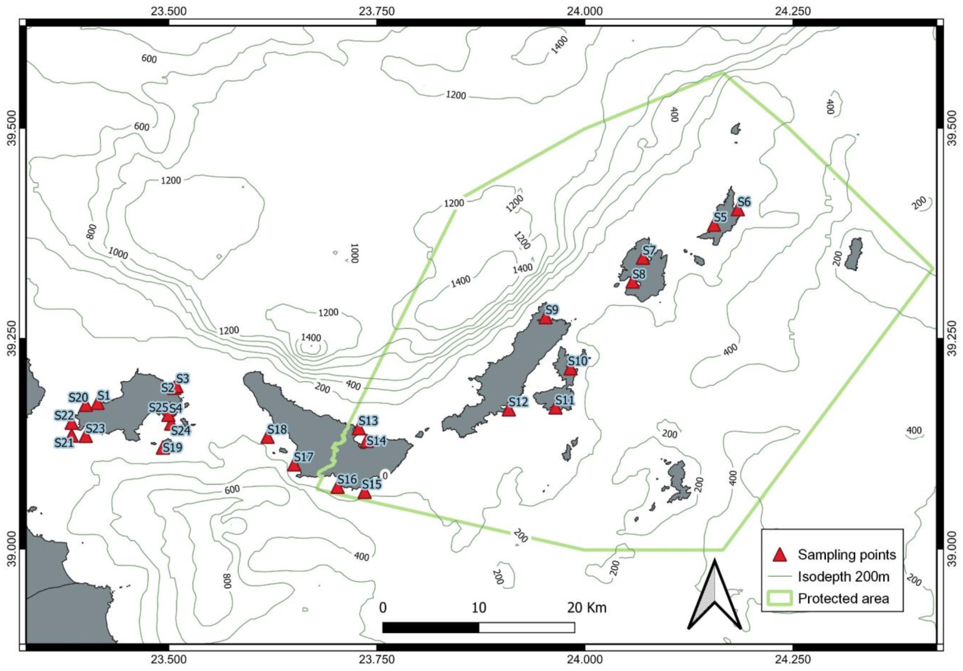
2.1. Study Area

The study area is an MPA included in the Natura 2000 network, belonging, administratively, to the region of Thessaly with Region Code GR1430004, named “National Marine Park of Alonissos—Northern Sporades, Eastern Skopelos” (NMPANS). The National Marine Park of Alonissos and Northern Sporades was the first MPA established in Greece and is currently the largest MPA in Europe, covering a surface area of 2500 km2 with 93.19% being a marine area (European Environmental Agency). The site has been designated as Special Areas of Conservation (SAC) since 2011. The NMPANS includes, besides Alonissos, the uninhabited islands of Kyra Panagia, Pappous, Gioura, Psathoura, Piperi, Peristera and Skantzoura, as well as 22 uninhabited islets and rocky outcrops (Figure 1). It is an ecologically sensitive area of international importance due to its unique natural features and is characterized by an exceptionally unique dynamics in natural and cultural environment [27].
The MPA is a natural habitat according to the Regional Unit of Magnesia and Sporades signed on 31 August 1986. It is considered an ideal place for study as it is geographically isolated, human interventions are minimal and it is a refuge for one of the most endangered marine species, the Mediterranean monk seal Monachus monachus [28]. Ministerial decisions were followed to protect the local natural reserve and in 1992 the area was declared as a National Marine Park. As of 25 May 2022 the National Marine Park of Alonissos Northern Sporades’ main goal is to combine the conservation of biodiversity, the management of climate crisis, the protection of ecosystems and to preserve its natural resources with the rise of socioeconomic growth and cohesion according to the principles of sustainable development and the surveillance of the entire area of the park on a daily basis, recording the environment conditions and controlling the activities in the area [29,30,31]. The climate is Mediterranean with very strong, dry, seasonal north winds called meltemia, which take place mostly in August, decreasing the summer temperatures, providing great visibility, causing turbulence in the sea and prevailing the limestone rocks [32,33].

2.2. In Situ Data

Remote sensing is an essential tool and offers several unique advantages, but also has some limitations. Although the spatial, temporal and spectral resolution of satellite sensors have been significantly improved, the mapping of benthic communities is limited by the penetration of radiation only into the visible region of the electromagnetic spectrum and the de facto spectral resolution, making benthic marine species segregation difficult [34,35].
In the marine environment, access and collection of data is a difficult task. A better study of in situ physical, chemical, and biological properties is often provided using conductivity temperature depth (CTD), achieving a more accurate perception of benthic communities. CTD nowadays offers unique capabilities to the scientific community. It is excessively used to investigate how physicochemical parameters and biological processes are related to the observed distribution and variation of ocean species and benefit ecological study.
Moreover, it provides high-resolution and very accurate data, while it can be used at depths up to several thousand meters. The limitation of CTD sampling is that only a point can be measured each time, and many casts, which are costly and time-consuming, are needed to acquire a broad picture of the marine environment of interest [36]. A series of in situ measurements were carried out inside and close to the study area (Figure 2). Vertical profiles of five physicochemical parameters of the sea water column (temperature, salinity, pH, dissolved oxygen, Chl-a) were considered and included in the analysis, having been measured by CTD at various depths, from the surface to the seafloor, at 21 sampling locations, between 20 and 22 May 2019. The abundance of Holothuria was counted with diving in the sampling points where CTD measurements were taken.

2.3. Satellite Database

Many global processes such as climate change, detection of biodiversity, eutrophication levels and water quality are based on sea surface temperature (SST) variability [37]. The SST is studied with the highest frequency of all other parameters and is one of the most critical and important indicators of physical, chemical and biological processes in the water column [38]. Chl-a is characterized as the “blood” of the plants, being directly involved in photosynthesis and one of the most important metabolic processes in the biosphere [39]. Observing Chl-a concentration provides vital information for studying and estimating water quality and its parameters, which is essential for marine ecosystems [40,41] and is systematically monitored by remotely sensed data [42,43]. Chl-a is used for determining marine primary production related to fisheries [44,45] and water resources management [46]. Particulate organic carbon (POC) is an important matter found in the ocean, contributing significantly to the marine carbon cycle [47,48,49] and playing a key role in the function of aquatic ecosystems [50,51]. It could be a good indicator of fish farming [52,53] and biological productivity in eutrophic [54] and euphotic zones of marine environments [55,56]. The biotic and detritus components of POC could be used as indicators of pollution [57,58,59].
SST, Chl-a and POC data from the moderate resolution imaging spectroradiometer (MODIS) of the Terra satellite were obtained from the official website of National Aeronautics and Space Administration [NASA] and Ocean Color Web (https://oceancolor.gsfc.nasa.gov/cgi/l3, 10 October 2021). These data are managed by the Ocean Biology Processing Group (OBPG) of the Goddard Space Flight Center (GSFC). MODIS combines satisfactory spectral, spatial, temporal and radiometric resolution and, generally, provides high-quality products of geophysical parameters which are produced by applying appropriate algorithms [60]. The time series utilized covered a period from 1 March 2000 to 29 February 2020 on a monthly basis since the launch of the satellite. Both daytime and night-time SSTs were considered in this work. The data at level 3 SMI (standard mapped image) products downloaded in netCDF (network common data form) (https://oceancolor.gsfc.nasa.gov/docs/technical/ocean_level3_smi_products.pdf, 3 November 2021).
All data have a spatial resolution of 4 km. The estimation of SST is based on the wavelength 11 μm and 12 μm used during daytime (from 31 to 32 channels) and night-time 3.9 μm and 4 μm (from 20, 22 and 23 channels). SST values are expressed in degrees Celsius (°C) and Chl-a and POC in mg/m3. A total of 960 Level-3 (SMI) products (240 for SST daytime, 240 for SST night-time, 240 for Chl-a and 240 for POC, each one representing a month for the 20-year period), were used for monthly SST, Chl-a and POC. Data were retrieved for the 128 pixels, enclosed by the polygon corresponding to the study area, excluding any terrestrial section, for all the parameters. The image processing was carried out with the SeaDAS 7.5.3 software. Further analysis and maps were created using the open source QGIS. The polygon that defines the study area was obtained from the official website of Natura 2000 network (Data Access–Natura 2000–Nature–Environment–European Commission (europa.eu, 8 September 2021)).

3. Results

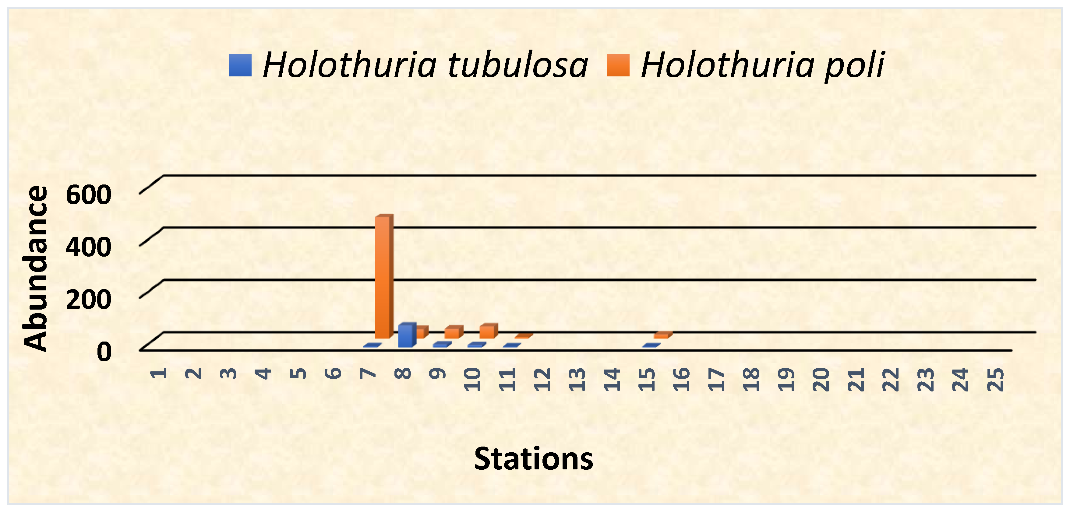
3.1. Species Abundance

The total number of locations sampled was 25, including 12 within the limits of the MPA (Figure 2), to estimate the abundance (number of animals over large areas). Two species of Holothuria were identified during the sampling carried out in the marine park, viz. Holothuria poli and Holothuria tubulosa. In this study, emphasis was given to the 12 sampling stations. Holothuria poli (Delle Chiaje, 1824), also known as the white spot cucumber, are members of the class Holothuroidea and are Mediterranean Sea cucumbers, benthic species, living within a depth range of 0 to 250 m [61]. The species occur in tropical and temperate regions, and are highly commercially important to Asian markets due to increased demand of consumption [62,63,64]. The reproductive cycle begins in July and is completed in September. During October and November there is no reproductive activity [65]. There are no scientific studies on the biology of the species and the available information is limited to its distribution in various areas of the Greek seas.
Evidence of fishery biology exists from the Turkish Aegean coast, where it is intensively fished and where it is probably the most densely populated species as it accounts for about 80% of total fishery production [66]. Holothuria tubulosa (Gmelin, 1788) is considered to be one of the most known Holothuria species and like all Holothuroidea family, it is a common benthic species of the Aegean coast, extending depth-wise from the upper sub-coastal zone, while its bathymetric distribution reaches 100 m depth [67] with a high abundance and distribution in the Atlantic Ocean and Eastern Mediterranean [68].
It lives on mobile substrates (phanerogamous grasslands, sandy, muddy and crumbly bottoms). Biology of these species has been extensively studied in populations of the Adriatic and Western Mediterranean basins, while corresponding information from the Aegean coast is limited [69]. The body size also shows a similar correlation. It is a gonochoristic species, without obvious sexual dimorphism, as only the examination of gonads is used to determine the sex of these organisms with a sex ratio ranging approximately 1:1. The species presented an annual reproductive cycle, with synchronous gonad development which begins in late spring peaking in summer. Its reproductive pattern shows a high correlation with water temperature [70,71]. Spawning occurs at the end of the summer season. More specifically, it begins in July and extends up to September. Between October and January, the species enter the resting phase [72]. In general, a total of 717 individual sea cucumbers were identified, with the most abundant being Holothuria poli (603) and the least Holothuria tubulosa (114) (Figure 3).

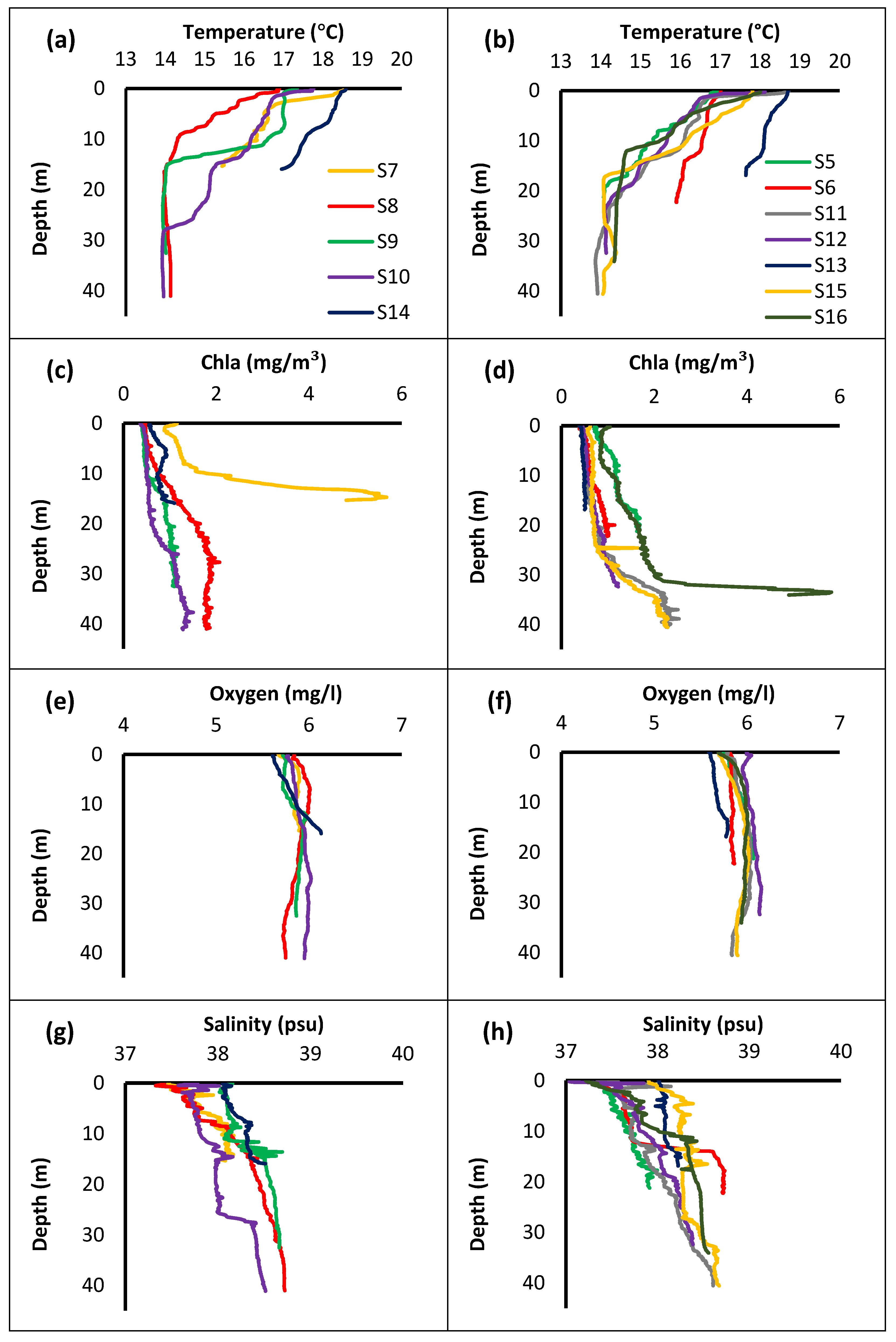
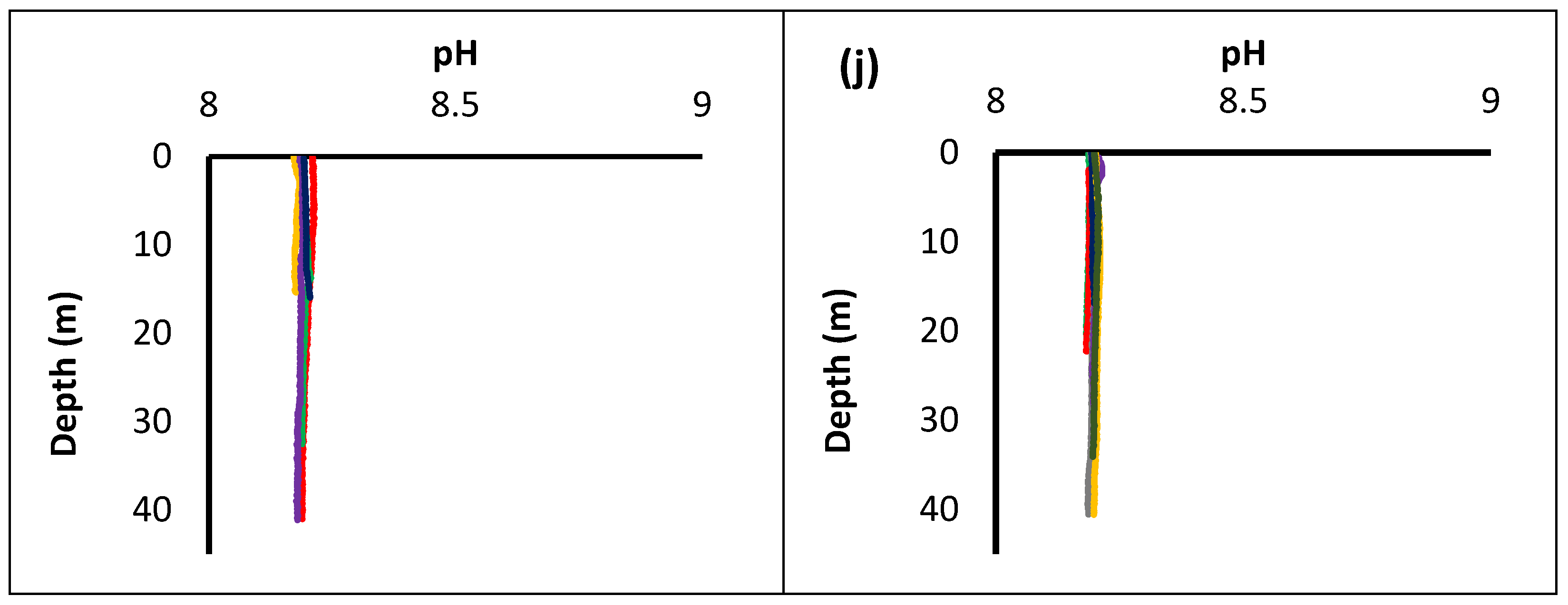
3.2. Physicochemical Parameters

In Figure 3, the values are organized into two groups. From Figure 4a–i the parameters correspond to locations where Holothuria species are found, while from Figure 4b–j where species were not identified. The analysis showed that in stations where sea cucumbers were noticed, temperature changes most rapidly near the surface. The highest peak observed at the surface decreases rapidly up to 10 to 15 m, where in most cases is stabilized. More specifically, at stations S7 and S14, temperature started to decline below 15 m while in other stations the decline started at ~10 m. Chl-a concentration showed a significant increase at station S7 where the most Holothuria were observed. Oxygen concentration showed a slight increase at station S14, compared to other stations. Values of salinity showed the same increased pattern with no major changes at all stations. As for pH, the variation was almost identical at all stations.
In stations where sea cucumbers were absent, the physical parameters showed a variation according to depth. Temperature showed minimum changes at stations S6 and S13 compared to other stations. On the other hand, Chl-a concentration increased rapidly at station S16 below 30 m, in contrast to other stations. Oxygen values remained almost the same at all stations. Salinity concentration increased rapidly over 38.5 psu in station S6, while at station S5 the recorded values of salinity were below 38 psu. At all other stations, there were not recorded any significant changes according to depth at salinity values. As for pH, no change was recorded whatsoever.

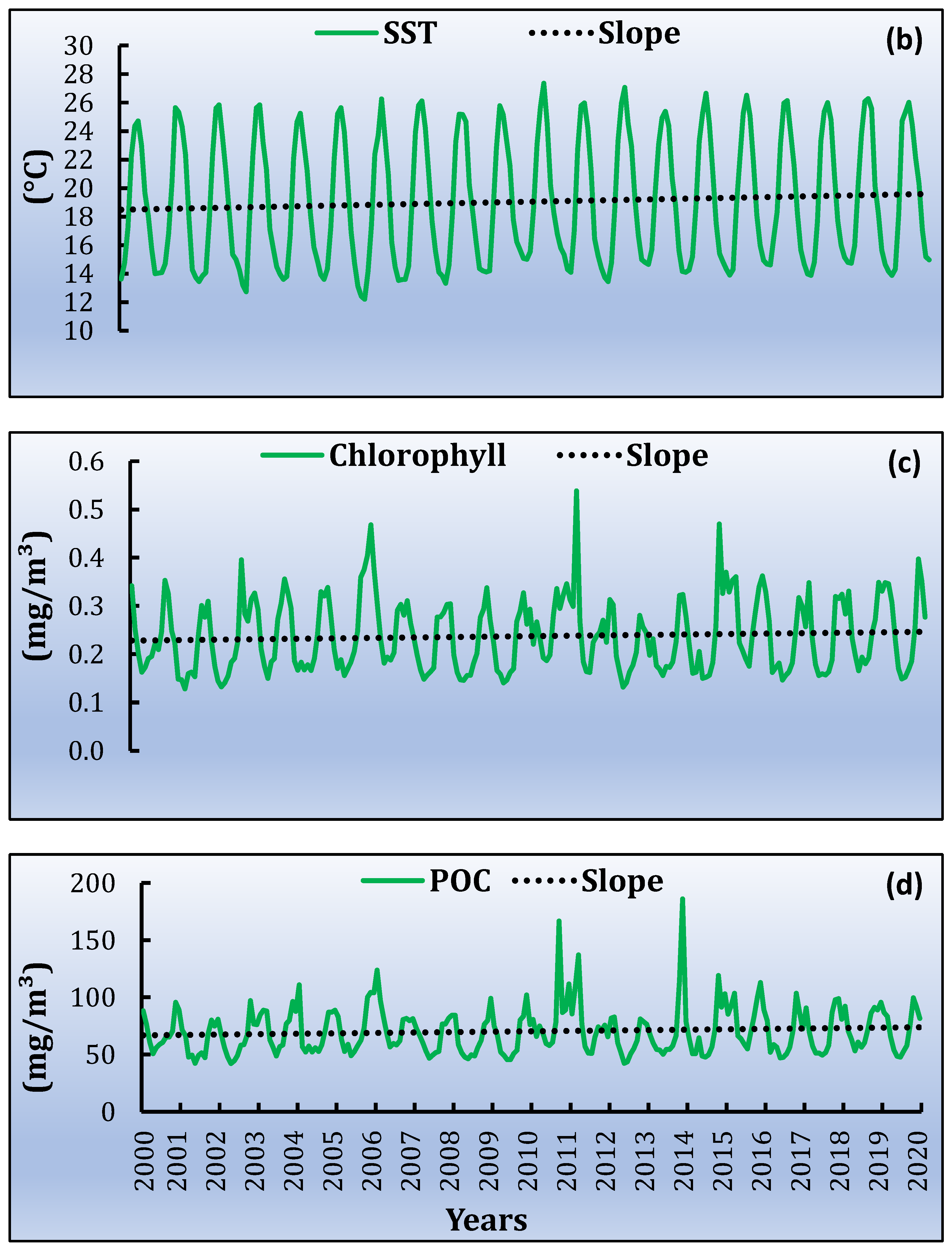
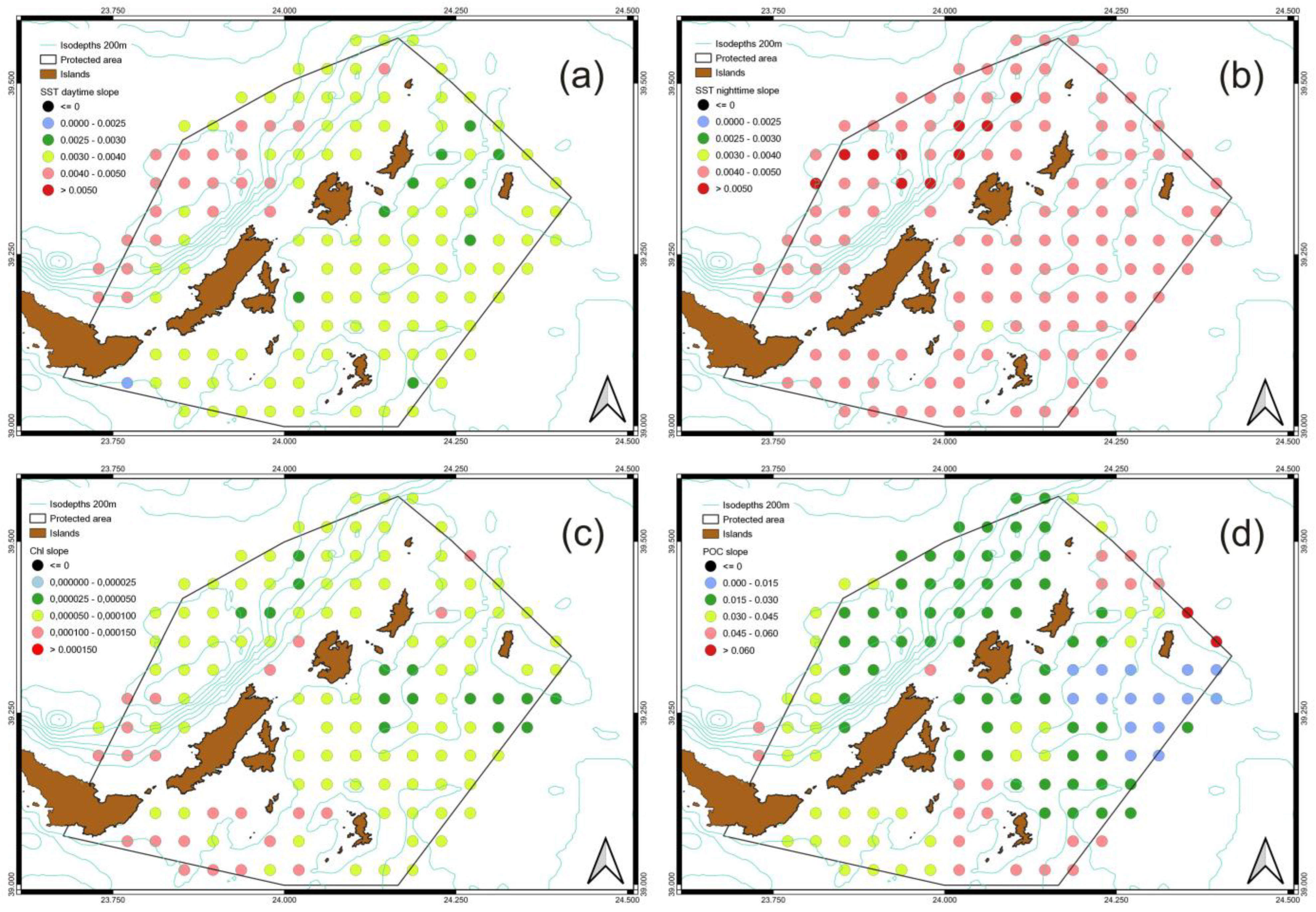
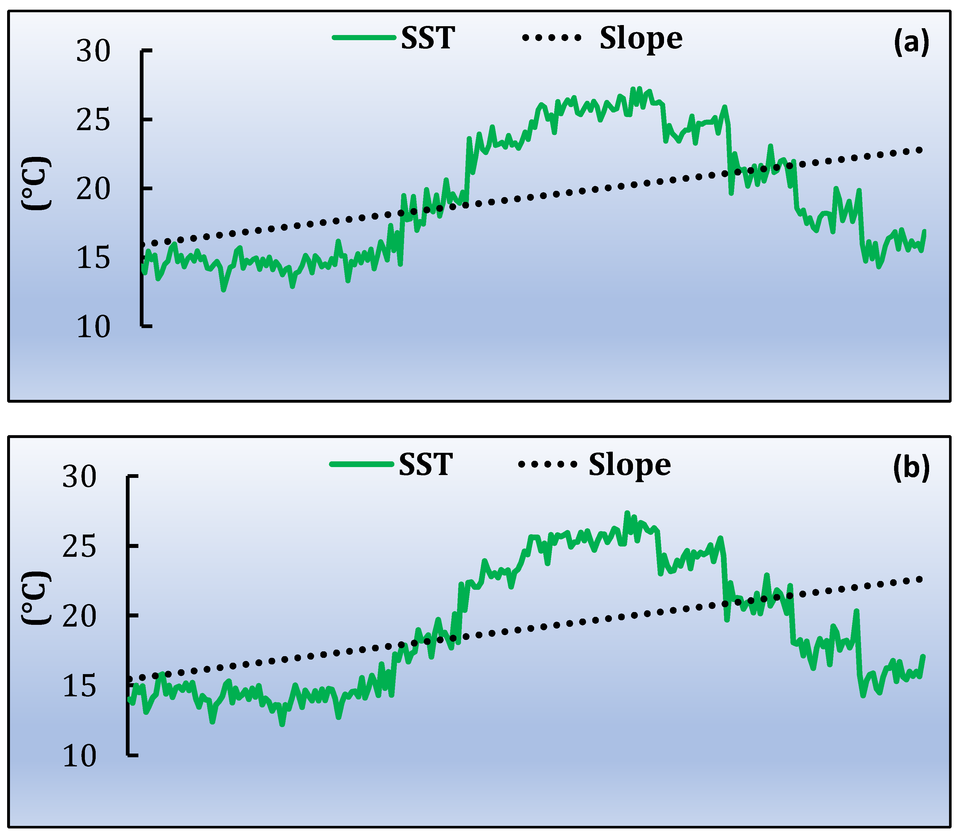
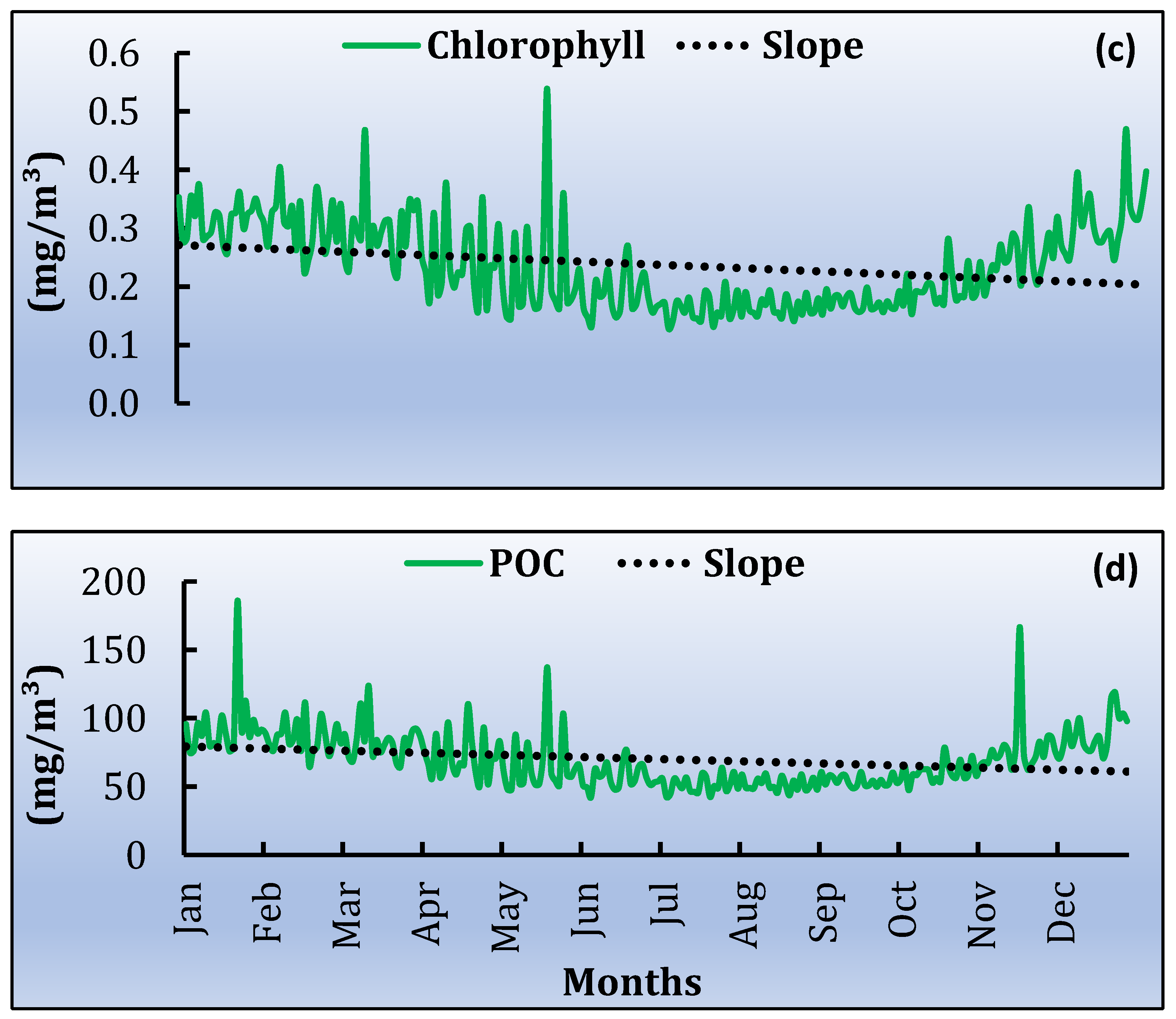
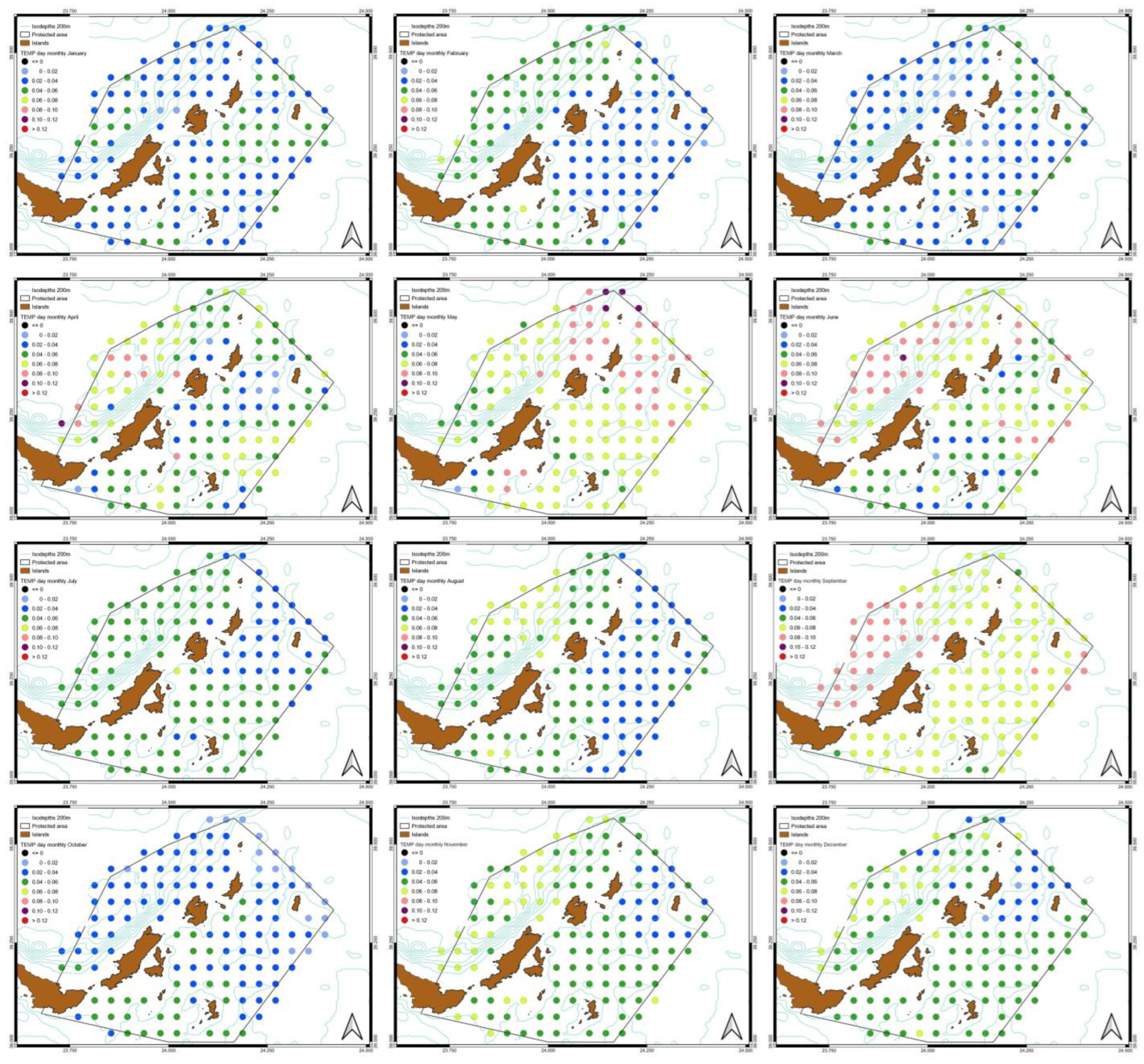
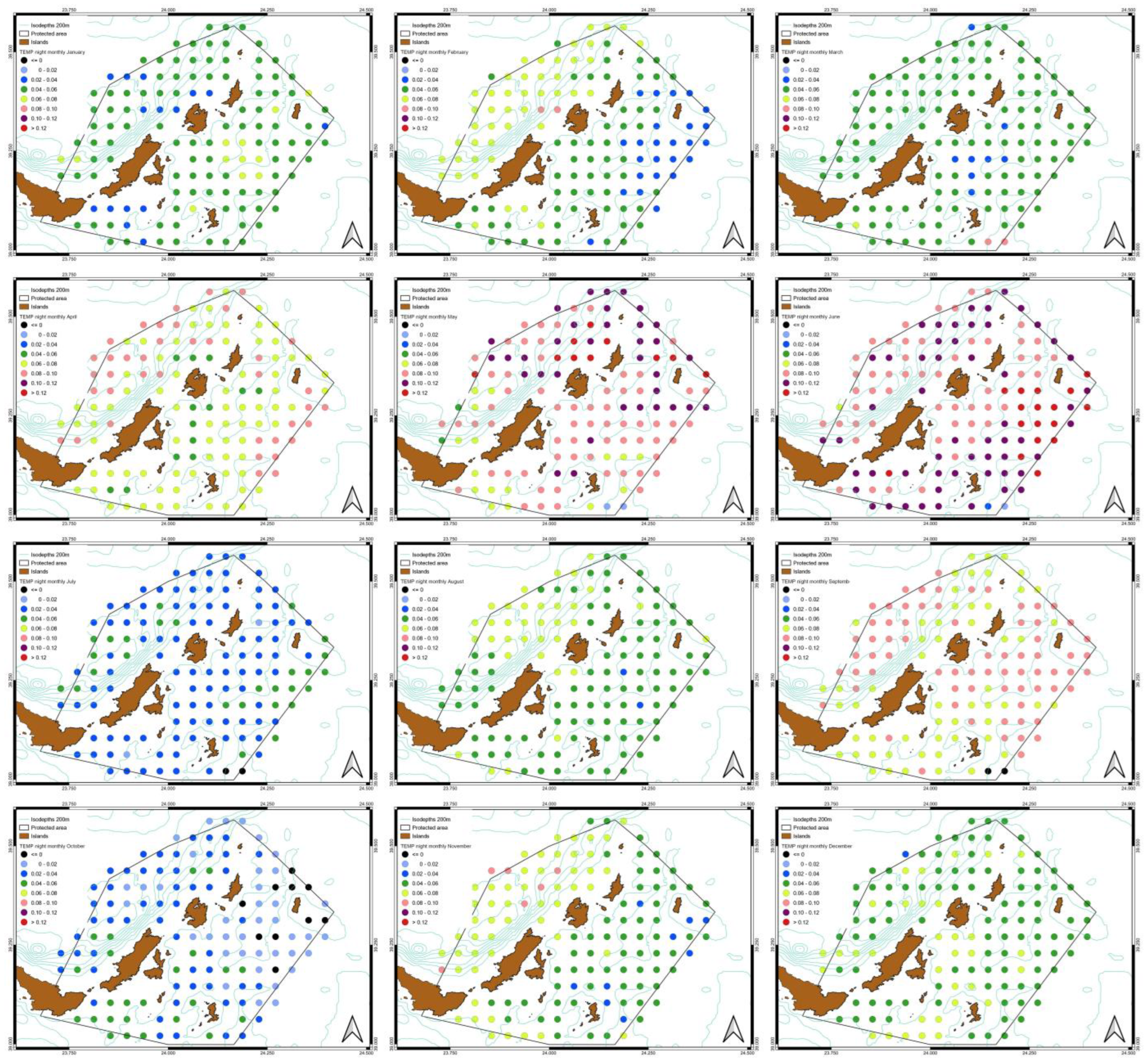
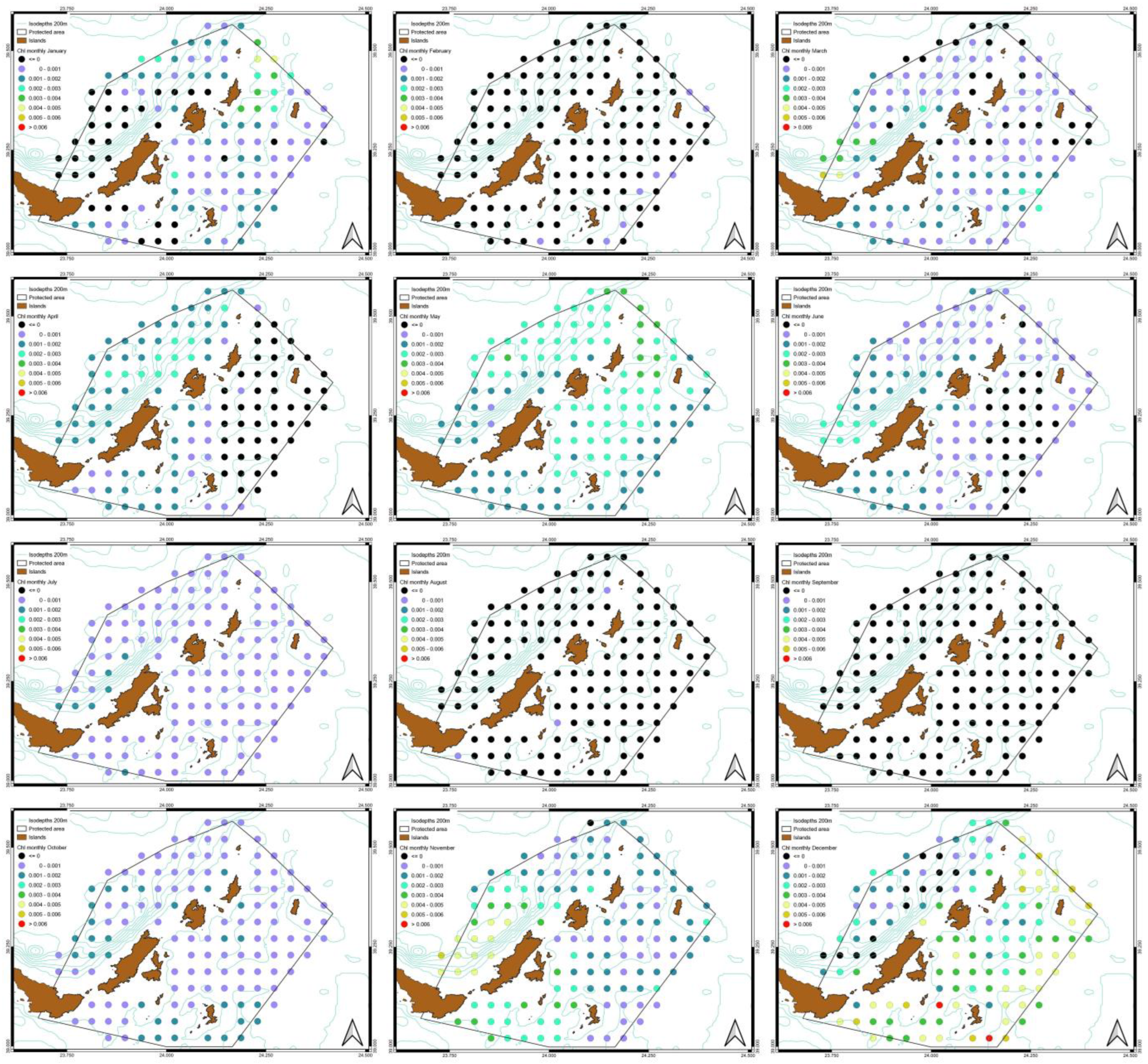
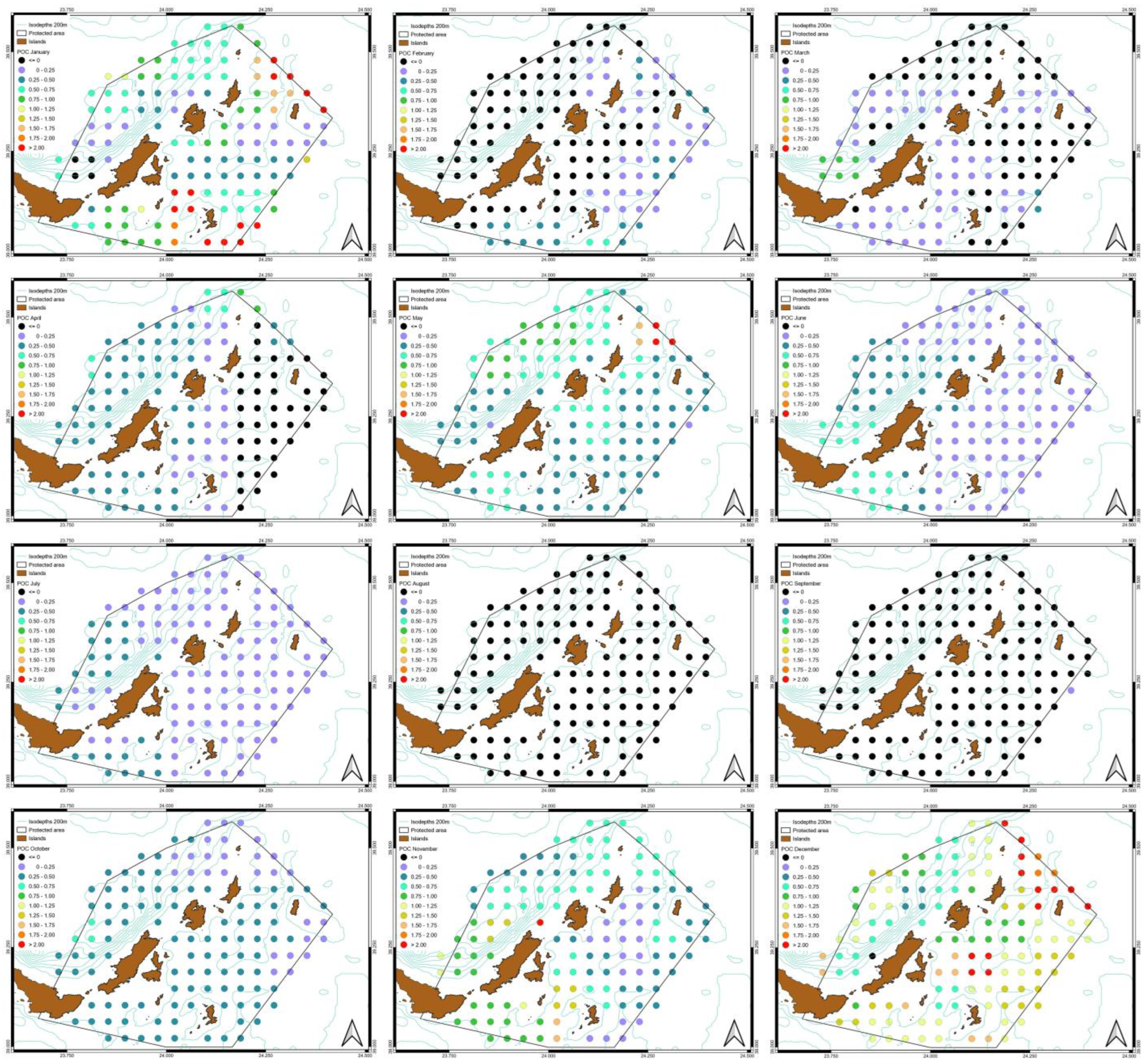
3.3. Spatiotemporal Variati Ons of SST, Chl-a and Particulate Organic Carbon [POC]

Based on the satellite products, the monthly time series was extracted. Firstly, the average values for the study area were estimated. The highest average daytime monthly SST value is observed in August (~28 °C) and the lowest during February (~11 °C). From the night-time dataset, the lowest SST is in March (12.8 °C) and the highest during August (~26.6 °C). In general, during the twenty-year time series, the maximum daytime SST values are mostly observed in August, during the warm period of July and August, while the lowest values are in February and March, for both daytime and night-time (Figure 5a,b). The mean monthly values of Chl-a concentration range between 0.092 mg/m3 and 0.879 mg/m3, during July 2001 and May 2011, respectively (Figure 5c). POC ranged from 42.184 mg/m3 to 186.044 mg/m3, following almost the same monthly pattern as for Chl-a. The highest concentration of POC was recorded in January 2014 and the lowest in June 2002 (Figure 5d).
As a second step, the slopes for the time series are estimated for each pixel of the MPA and for each parameter. The slope was averaged over the entire study area for SST daytime, SST night-time, Chl-a and POC. In all cases a positive trend (Figure 5) is observed. The linear trends, for the whole time series, are 0.029 ± 0.007 °C/year and 0.030 ± 0.007 °C/year during daytime and night-time, respectively (Figure 5a,b). For Chl-a, the linear trend is 0.000076 ± 0.00014 mg/m3/year (Figure 5c) and for POC 0.029 ± 0.038 mg/m3/year (Figure 5d). All the trends provided are statistically significant at the 95% level [p ≤ 0.05]. Table 1 shows the increased min and max values during the twenty years. Figure 6 shows the spatial distribution of the slope for the four parameters. Each dot corresponds to the center of the pixel. The mean SST slope for daytime, of the entire study region, reveals a clear increasing trend in the north-western part of the MPA while the same increasing trend is observed in night-time as well. However, the increasing SST trend is stronger during night-time compared to daytime. Meanwhile, the Chl-a slope distribution shows an increasing trend in the southwest part of the MPA (Figure 6c). POC slope concentration is increased in north-eastern and southern part of the MPA during the whole time series.
The average monthly SST slope during daytime shows that lowest values usually occur during the cold season (winter–autumn), while in warm season (summer–spring) it the highest values of SST slope are observed, especially in the northwest part of the MPA. For the whole time series, the highest increase of the SST slope is observed in the western and north-western part of the MPA. Spatially, Chl-a concentration is increased mainly in the south-western part of the MPA, while there are some regions at the center of the study area where high increases are observed during the whole time series. The POC slope shows its highest peak in the southeastern and north-eastern part of the marine park (Figure 6d).
In Figure 7, the time series for each month are separated. For SST the variation does not exhibit any extreme values between the months for all the years. For Chl-a and POC, the values vary significantly according to the month and among the years. For example, the Chl-a for May is much greater than any other month and for one year exceeds any other month. Only for July, August and September the variations are low compared to the other months for both Chl-a and POC. Although this refers to the averaged values for the whole study area, it implies a considerable variation among months, which should be considered. The study, therefore, carries on examining trends for all parameters on a monthly basis, resulting in Figure 8, Figure 9, Figure 10 and Figure 11. From these Figures, the values of slopes are different from those of the entire time series, for all parameters. For example, the diversification between regions, as shown in Figure 6 and Figure 11, exhibits a different pattern.
The monthly SST slope in night-time shows an overall greater increase compared to daytime during the 20-year study period (Figure 8 and Figure 9). The Chl-a slope shows a difference between the cold and warm season. Specifically, during September, October and February there was a decrease in values in the whole study area, while for the rest of the months there was an increasing trend, especially in the north and northwest areas, with an exception for December, where the highest peak was observed in southeast part of the MPA (Figure 10).
The monthly POC slope shows a negative increase during August and September, while a greater increasing trend is observed especially in December, January, November and May, mostly in the northeast part of the study area. In February, there is a negative increase in the northwest part, in March a negative increase in north and east part, while in April there is a negative increase in the whole east part of the MPA (Figure 11).

4. Discussion

MPAs are ideal places for studying sea cucumbers, as their diversity is higher due to lack of human activity [73]. There are specific species that show more abundance, as they are perfectly adapted to some habitats, preventing other species from living there and enhancing their reproduction rate [74]. Although the maturity of sea cucumbers is affected by environmental conditions, the relationship between multiple oceanographic factors does not cause any impact on the reproduction rate [75]. Multiple factors could play an influential role in the growth and survival of juvenile sea cucumbers. Depth and ocean acidification can decrease the population of Holothuria [76,77]. On the contrary, different types of reefs may constitute an ideal place for their growth [78]. The mass of sea cucumbers is increased by depth [79]. The salinity may be affected by atmospheric evaporation and freshwater influxes, at the same time. The relationships among all these variables may be impacted by other factors as well, as they are not exclusive to each other.
“Increasing air temperature will increase water temperature and deteriorate water quality conditions by accelerating the eutrophication process in water bodies, which in turn could cause environmental and health related issues” [80]. Moreover, the interaction between oceanic variables could have a direct impact on aquatic organisms, e.g., the SST and Chl-a presented an opposite correlation [81]. All these conditions create a complex environment for the planning of sampling and monitoring, especially for benthic species. Thus, it is important for a marine biologist to be able to identify candidate areas for studying, especially in the face of climate change. As the development and spread of species is not an “instantaneous” situation, but the result of a long process, it was chosen to study the trend of oceanic physicochemical parameters extracted from satellite data. This study was organized within and around an MPA, where in situ measurements (CTD and diving) were performed in the water column, important parameters for the existence of sea cucumbers were recognized, and, finally, the use of satellite products over a twenty-year period were examined in terms of the species abundance. This gives us a “superficial” indication of what prevails in the benthic substrate. During the diving process, no Holothuria was recorded for most sampling stations. In a few sampling stations two species were recorded, viz. Holothuria poli and Holothuria tubulosa. The growth rate of Holothuria tubulosa is increased under low water turbulence environments [82] and its population can be developed where organic accumulation is increased [83].
Water temperature plays a fundamental role in the growth of some Holothuria species (the higher the temperature, the greater the growth) rather than their survival [84]. For some other sea cucumber species (Apostichopus japonicus) the high-water temperatures (>20 °C) negatively affect their feeding and growth. At this higher temperature, they enter the aestivating phase, while the ideal temperature for these organisms to be maintained ranges between 14 °C and 15 °C [85]. Spawning (the process where the eggs and sperm are deposited into water) in some Holothuria (Holothuria arguinensis) can be provoked during periods of high temperature while gametogenesis (the process by which germ cells are produced in an organism) occurred in periods of low range of temperature [86]. For other species (e.g., Australostichopus mollis), temperatures higher than 24 °C can be lethal, negatively affecting growth and feeding rates [87]. In the study area, the CTD measurements range between ~17 °C–~19 °C in both cases and below 15 m the values are “stabilized” at ~14 °C. For each station, where Holothuria were found, there is a different degree of temperature reduction (thermocline). Salinity is one of the most important environmental factors with a tremendous impact on sea cucumbers, affecting their feeding, growth, survival and their abundance in general [88,89]. Salinity at 30 and 45 ppt has a negative impact on growth of Holothuria tubulosa, while Holothuria poli presents an increase in growth rate during summer and winter. At a temperature of 15 °C and salinity of 30 and 45 ppt the juveniles entered the aestivation phase and there is a decline in their mass. The highest specific growth and survival rate are obtained at salinity of 38 ppt in winter conditions [15 °C] for both species, while a temperature of 25 °C and a salinity in the range of 38–45 ppt for Holothuria poli and 38 ppt for Holothuria tubulosa during summer are considered as optimum values. A salinity of 25 ppt turns out to be deadly for both species, but such values were not recorded in the sampling area. Holothuria poli juveniles can adapt better in higher salinities than Holothuria tubulosa, increasing its survival rate [90].
Salinity did not increase over 38 pst in S7, where the highest abundance of Holothuria was recorded, as it is the optimal level for these species. For all the sample stations the vertical values of salinity were very similar in the range 38–39 ppt, indicating that there is no negative influence on the abundance. In terms of salinity, the conditions are more favorable for Holothuria poli, but this does not seem to influence significantly in this study area. At the sea surface there are variations of salinity that might be affected by the evaporation, as SST is increased. Therefore, there is no further need for using satellite data related to salinity.
Regarding the SST, as one of the key factors, satellite data is analyzed for the whole time series and for each month individually. On average, the SST trend of each pixel throughout the study area, from daytime and night-time satellite images, shows that the trend maintains its positive sign in the 20-year period, which generally implies an increase of SST. This is in accordance with an SST rise observed in the whole Mediterranean Sea during the last decades [91,92,93,94,95]. For the whole time series, a higher increase is observed in SST values during daytime in the western to northern parts, compared to the rest of the MPA; generally, there is a greater increase during night-time compared to daytime.
Studying the monthly trend of SST, during daytime, the trend of SST shows greater increase especially in May in the Northeast part of the MPA and in June in the western part. On the other hand, during night-time, an increasing trend is observed, except from October, in few areas in the eastern region and in small areas southeast in September. The highest increase is observed during May in the northeast part of the MPA and in June throughout the whole region. The SST slope shows significant seasonal variability. The highest increase for the whole time series, for both daytime and night-time, occurs during September, while the lowest is during October. A possible cause could be the weakening of the summer Etesian winds over the eastern Mediterranean [96,97,98], along with the sea heat capacity. For Holothuria tubulosa, feeding activity is increased during summer temperatures and is more energetic during night-time [99]. The higher increase occurs in night-time during their feeding activity and the higher trend is during May and June. This might be an indication that the feeding activity is moving to the end of spring and beginning of summer.
Sea cucumbers consume a high amount of oxygen, needed during reproduction [100]. Similar studies showed that pH and Chl-a increased due to the presence of sea cucumbers, while it was observed that low levels of dissolved oxygen consumptions were probably caused by the decomposition of organic matter. Furthermore, it was noted that sea cucumbers caused the increase of oxygen during their feeding. Chl-a showed an increase in oligotrophic environments [101]. In the study area, the vertical profile of pH values is similar for all the sampling stations. However, this is not the case for Chl-a, where there are variations. At S7, where most Holothuria species were recorded, Chl-a concentration increased rapidly five times up to 15 m, compared to other stations, where no significant changes were noticed. Below 15 m there is an increase of Chl-a in higher depths [>30 m], but in an area where no Holothuria were found. This can be justified since sea cucumbers need a lot of organic matter for their feeding activity and growth.
For Chl-a concentration, as recorded by the satellite data, there was a slight increase from 2000 to 2020, especially in western and south-western part of the MPA and close to the areas with abundance as well. The average monthly distribution of Chl-a shows high peaks in May reaching, in a case, over 0.5 mg/m3 and for the following months there is a decline. High concentrations are observed from November to April and the lowest value is shown in June. Therefore, during spring and winter periods the trend of concentration of Chl-a is at its highest level. The monthly slope of Chl-a indicates the highest increase mainly during May following with “patches” during June and winter months.
Similar results of another research on Holothuria tubulosa showed the effects of oceanographic parameters. More specifically, for temperature, the best specific growth rate (SGR) was recorded at 25 °C, while the lowest SGR at 30 °C and the negative SGR at 15 °C, because at these specific temperatures, sea cucumbers start to aestivate and hibernate, respectively. As for pH, this was between 7–7.8, which is optimum for breeding. Meanwhile, oxygen values ranged from 7.2 to 8.5 mg/L. Salinity concentration was increased due to evaporation [102]. POC is a food source for aquatic organisms. The POC concentration increases when sea cucumbers are in the state of low metabolic process (aestivation in summer and hibernation in winter period) and decreases in the feeding periods, showing that sea cucumbers successfully absorb nutrients (such as macroalgae), from organic matters in benthic environments, as they constitute important substances for their growth and enhancement [103,104]. The study of average monthly variations showed that the highest peak was observed during January and November with over 180 mg/m3 and 160 mg/m3, respectively, followed by May, while the minimum monthly average value is noticed in June. In areas where the sea cucumbers are recorded, the trend of POC is medium to low. The highest abundance was found on the center and northern part of the Kyra Panagia Island, at the S7 and S8, where POC has not shown a significant increase. In general, POC concentration indicates a noticeably larger increase compared to Chl-a during the twenty-year time, especially in the northeastern and southern part of the MPA during the whole time series. The same pattern is observed in areas close to where Holothuria was found. The monthly slope pattern indicates, in general, an increase during January, April, May and June, close to areas where Holothuria are spotted. This is an indication for POC availability for feeding.

5. Conclusions

Extensive studies of physicochemical parameters could improve our knowledge on marine biodiversity and its dependence on environmental factors. The use of satellite data could contribute significantly to the study of the interaction between oceanographic parameters and the biology of benthic species (Holothuria) in coastal environments. Among the parameters, which are vital to Holothuria, some are already available as products from satellite data (such as SST, Chl-a and POC), providing information about their trend for a long-term period. Examining only the average values for the whole study area and annual variations of the parameters did not show any specific indication about the abundance. Their spatiotemporal variability is of great importance for the environmental biology of the benthic species. In order to identify areas with higher abundance, the study is focused on monthly variations on a pixel basis. Areas where there is an increasing trend in concentration of POC, are places for the development of sea cucumber species. The rise of SST, in the long term, due to climate change, could create a warmer environment and probably negatively affect the activities of sea cucumbers. This analysis could be the basis for comparative studies in the future.

Author Contributions

Conceptualization, C.D. and D.V.; methodology, C.D.; software, C.D.; formal analysis, P.C. and C.D.; investigation, P.C.; resources, D.V.; data curation, P.C. and C.D.; writing—original draft preparation, P.C.; writing—review and editing, P.C. and C.D.; visualization, C.D. and N.N.; supervision, C.D. and D.V.; funding acquisition, D.V. All authors have read and agreed to the published version of the manuscript.

Funding

This research was partially supported by the European Union, in the context of the Operational Program for Maritime and Fisheries 2014–2020 and are co-financed by the European Maritime and Fisheries Fund (EMFF) and the Greek Government (GR). The contribution rates of EMFF and GR to the total public expenditure have been established by applying Article 95 of Regulation (EU) 508/2014 and correspond to 75% EMFF and 25% GR. The project entitled “Exploitation and management of sea cucumber fisheries (Holothuria spp.): processing (food and biotech products) and safeguarding of stocks” with project code MIS 5010720.

Institutional Review Board Statement

Not applicable.

Informed Consent Statement

Not applicable.

Data Availability Statement

The part data presented in this study are available on request from the corresponding author.

Acknowledgments

We would like to express our gratitude to NASA Goddard Space Flight Center, Ocean Ecology Laboratory, Ocean Biology Processing Group; (2018): Sea-viewing Wide Field-of-view Sensor (SeaWiFS) Ocean Color Data, NASA OB. DAAC for providing MODIS data and SeaDAS 7.5.3 software package.

Conflicts of Interest

The authors declare no conflict of interest.

References

  1. Day, J.; Dudley, N.; Hockings, M.; Holmes, G.; Laffoley, D.; Stolton, S.; Wells, S.; Wenzel, L. Guidelines for Applying the IUCN Protected Area Management Categories to Marine Protected Areas, 2nd ed.; World Comission on Protected Areas: Gland, Switzerland, 2019; ISBN 9782831719412. [Google Scholar]
  2. Reuchlin-Hugenholtz, E.; McKenzie, E. Marine Protected Areas: Smart Investments in Ocean Health; Tanzer, J., Ed.; WWF: Gland, Switzerland, 2015; ISBN 9782940529216. [Google Scholar]
  3. Bertzk, B.; Corrigan, C.; Kemsey, J.; Kenney, S.; Ravilious, C.; Besançon, C.; Burgess, N. Protected Planet Report 2012: Tracking Progress Towards Global Targets for Protected Areas; IUCN: Gland, Switzerland, 2012; ISBN 9789280731897. [Google Scholar]
  4. Sala, E.; Giakoumi, S. No-Take Marine Reserves Are the Most Effective Protected Areas in the Ocean. ICES J. Mar. Sci. 2018, 75, 1166–1168. [Google Scholar] [CrossRef] [Green Version]
  5. Wang, F.; Wang, Y.; Chen, Y.; Liu, K. Remote sensing approach for the estimation of particulate organic carbon in coastal waters based on suspended particulate concentration and particle median size. Mar. Pollut. Bull. 2020, 158, 111382. [Google Scholar] [CrossRef] [PubMed]
  6. Jia, C.; Minnett, P.J. High latitude sea surface temperatures derived from MODIS infrared measurements. Remote Sens. Environ. 2020, 251, 112094. [Google Scholar] [CrossRef]
  7. Minnett, P.J.; Alvera-Azcárate, A.; Chin, T.M.; Corlett, G.K.; Gentemann, C.L.; Karagali, I.; Li, X.; Marsouin, A.; Marullo, S.; Maturi, E.; et al. Half a Century of Satellite Remote Sensing of Sea-Surface Temperature. Remote Sens. Environ. 2019, 233, 111366. [Google Scholar] [CrossRef]
  8. Kilpatrick, K.A.; Podestá, G.; Walsh, S.; Williams, E.; Halliwell, V.; Szczodrak, M.; Brown, O.B.; Minnett, P.J.; Evans, R. A decade of sea surface temperature from MODIS. Remote Sens. Environ. 2015, 165, 27–41. [Google Scholar] [CrossRef]
  9. Pahlevan, N.; Smith, B.; Binding, C.; Gurlin, D.; Li, L.; Bresciani, M.; Giardino, C. Hyperspectral retrievals of phytoplankton absorption and chlorophyll-a in inland and nearshore coastal waters. Remote Sens. Environ. 2021, 253, 112200. [Google Scholar] [CrossRef]
  10. Otsuka, A.Y.; Feitosa, F.A.N.; Flores-Montes, M.J.; Silva, A. Dynamics of Chlorophyll a and Oceanographic Parameters in the Coastal Zone: Barra das Jangadas-Pernambuco, Brazil. J. Coast. Res. 2016, 32, 490–499. [Google Scholar] [CrossRef]
  11. Fan, H.; Wang, X.; Zhang, H.; Yu, Z. Spatial and temporal variations of particulate organic carbon in the Yellow-Bohai Sea over 2002–2016. Sci. Rep. 2018, 8, 7971. [Google Scholar] [CrossRef] [Green Version]
  12. Guan, Q.; Feng, L.; Hou, X.; Schurgers, G.; Zheng, Y.; Tang, J. Eutrophication changes in fifty large lakes on the Yangtze Plain of China derived from MERIS and OLCI observations. Remote Sens. Environ. 2020, 246, 111890. [Google Scholar] [CrossRef]
  13. Zhang, L.; Liao, Q.; Gao, R.; Luo, R.; Liu, C.; Zhong, J.; Wang, Z. Spatial variations in diffusive methane fluxes and the role of eutrophication in a subtropical shallow lake. Sci. Total Environ. 2021, 759, 143495. [Google Scholar] [CrossRef]
  14. Henryson, K.; Kätterer, T.; Tidåker, P.; Sundberg, C. Soil N2O emissions, N leaching and marine eutrophication in life cycle assessment—A comparison of modelling approaches. Sci. Total Environ. 2020, 725, 138332. [Google Scholar] [CrossRef] [PubMed]
  15. Fernandez, J.M.; Townsend-Small, A.; Zastepa, A.; Watson, S.B.; Brandes, J.A. Methane and nitrous oxide measured throughout Lake Erie over all seasons indicate highest emissions from the eutrophic Western Basin. J. Great Lakes Res. 2020, 46, 1604–1614. [Google Scholar] [CrossRef]
  16. Chen, Q.; Huang, M.; Tang, X. Eutrophication assessment of seasonal urban lakes in China Yangtze River Basin using Landsat 8-derived Forel-Ule index: A six-year (2013–2018) observation. Sci. Total Environ. 2020, 745, 135392. [Google Scholar] [CrossRef]
  17. Chen, Z.; Huang, P.; Zhang, Z. Interaction between carbon dioxide emissions and eutrophication in a drinking water reservoir: A three-dimensional ecological modeling approach. Sci. Total Environ. 2019, 663, 369–379. [Google Scholar] [CrossRef] [PubMed]
  18. Rajendran, S.; Vethamony, P.; Sadooni, F.N.; Al-kuwari, H.A.; Al-khayat, J.A.; Seegobin, V.O.; Govil, H.; Nasir, S. Detection of Wakashio oil spill off Mauritius using Sentinel-1 and 2 data: Capability of sensors, image transformation methods and. Environ. Pollut. 2021, 274, 116618. [Google Scholar] [CrossRef]
  19. Balogun, A.L.; Yekeen, S.T.; Pradhan, B.; Wan Yusof, K.B. Oil spill trajectory modelling and environmental vulnerability mapping using GNOME model and GIS. Environ. Pollut. 2021, 268, 115812. [Google Scholar] [CrossRef] [PubMed]
  20. Nelson, J.R.; Grubesic, T.H. A spatiotemporal analysis of oil spill severity using a multi-criteria decision framework. Ocean Coast. Manag. 2021, 199, 105410. [Google Scholar] [CrossRef]
  21. Obida, C.B.; Blackburn, G.A.; Whyatt, J.D.; Semple, K.T. Counting the cost of the Niger Delta’s largest oil spills satellite remote sensing reveals extensive environmental damage with 1million people in the impact zone. Sci. Total Environ. 2021, 775, 145854. [Google Scholar] [CrossRef]
  22. Klemas, V. Remote sensing techniques for studying coastal ecosystems: An overview. J. Coast. Res. 2011, 27, 2–17. [Google Scholar] [CrossRef]
  23. Ferreira, M.A.; Andrade, F.; Mendes, R.N.; Paula, J. Use of satellite remote sensing for coastal conservation in the eastern african coast: Advantages and shortcomings. Eur. J. Remote Sens. 2012, 45, 293–304. [Google Scholar] [CrossRef]
  24. Namukose, M.; Msuya, F.E.; Ferse, S.C.A.; Slater, M.J.; Kunzmann, A. Growth performance of the sea cucumber Holothuria scabra and the seaweed Eucheuma denticulatum: Integrated mariculture and effects on sediment organic characteristics. Aquac. Environ. Interactactions 2016, 8, 179–189. [Google Scholar] [CrossRef] [Green Version]
  25. Parra-luna, M.; Martín-pozo, L.; Hidalgo, F.; Zafra-Gómez, A. Common sea urchin (Paracentrotus lividus) and sea cucumber of the genus Holothuria as bioindicators of pollution in the study of chemical contaminants in aquatic media. A revision. Ecol. Indic. 2020, 113, 106185. [Google Scholar] [CrossRef]
  26. Mezali, K.; Soualili, D.L. The Ability of Holothurians to Select Sediment Particles and Organic Matter. SPC Beche Mer Inf. Bull. 2013, 1, 38–43. [Google Scholar]
  27. Kovos, D.; Karagiannis, G. Field study on the “National Marine Park” of Alonissos, Greece. J. Tour. Res. 2018, 19, 243–253. [Google Scholar]
  28. Karamanlidis, A.A.; Androukaki, E.; Adamantopoulou, S.; Chatzispyrou, A.; Johnson, W.M.; Kotomatas, S.; Papadopoulos, A.; Paravas, V.; Paximadis, G.; Pires, R.; et al. Assessing Accidental Entanglement as a Threat to the Mediterranean Monk Seal Monachus Monachus. Endanger. Species Res. 2008, 5, 205–213. [Google Scholar] [CrossRef]
  29. Oikonomou, Z.-S.; Dikou, A. Integrating Conservation and Development at the National Marine Park of Alonissos, Northern Sporades, Greece: Perception and Practice. Environ. Manag. 2008, 42, 847–866. [Google Scholar] [CrossRef]
  30. Konaxis, I. Alonissos Island and the Northern Sporades Marine National Park as a Strategic Socio-Economic Node for The Culture of the Aegean Sea. Am. Res. J. Humanit. Soc. Sci. 2020, 3, 49–53. [Google Scholar]
  31. Trivourea, M.N.; Karamanlidis, A.A.; Tounta, E.; Dendrinos, P.; Kotomatas, S. People and the Mediterranean Monk Seal (Monachus monachus): A Study of the Socioeconomic Impacts of the National Marine Park of Alonissos, Northern Sporades, Greece. Aquat. Mamm. 2011, 37, 305–318. [Google Scholar] [CrossRef] [Green Version]
  32. Androulidakis, Y.S.; Krestenitis, Y.N.; Psarra, S. Coastal upwelling over the North Aegean Sea: Observations and simulations. Cont. Shelf Res. 2017, 149, 32–51. [Google Scholar] [CrossRef]
  33. Poulos, S.E.; Drakopoulos, P.G.; Collins, M.B. Seasonal variability in sea surface oceanographic conditions in the Aegean Sea (Eastern Mediterranean): An overview. J. Mar. Syst. 1997, 13, 225–244. [Google Scholar] [CrossRef]
  34. Al-Wassai, F.A.; Kalyankar, N.V. Major Limitations of Satellite images. J. Glob. Res. Comput. Sci. 2013, 4, 51–59. [Google Scholar]
  35. Gao, J. Bathymetric mapping by means of remote sensing: Methods, accuracy and limitations. Prog. Phys. Geogr. 2009, 33, 103–116. [Google Scholar] [CrossRef]
  36. Lawson, K.; Larson, N.G. CTD. In Encyclopedia of Ocean Sciences; Steele, J.H., Ed.; Sea-Bird Electronics Inc.: Bellevue, DC, USA, 2001; pp. 579–588. ISBN 9780122274305. [Google Scholar]
  37. Fingas, M. Remote Sensing for Marine Management, 2nd ed.; Elsevier: Amsterdam, The Netherlands, 2018; ISBN 9780128050521. [Google Scholar]
  38. Lotfinasabasl, S.; Gunale, V.R.; Khosroshahi, M. Applying geographic information systems and remote sensing for water quality assessment of mangrove forest. Acta Ecol. Sin. 2018, 38, 135–143. [Google Scholar] [CrossRef]
  39. Cai, J.-Q.; Liu, X.-M.; Gao, Z.-J.; Li, L.-L.; Wang, H. Chlorophylls derivatives: Photophysical properties, assemblies, nanostructures and biomedical applications. Mater. Today 2021, 45, 77–92. [Google Scholar] [CrossRef]
  40. Nazeer, M.; Nichol, J.E. Development and application of a remote sensing-based Chlorophyll-a concentration prediction model for complex coastal waters of Hong Kong. J. Hydrol. 2016, 532, 80–89. [Google Scholar] [CrossRef]
  41. Yu, X.; Shen, J. A data-driven approach to simulate the spatiotemporal variations of chlorophyll-a in Chesapeake Bay. Ocean Model. 2021, 159, 101748. [Google Scholar] [CrossRef]
  42. Chawla, I.; Karthikeyan, L.; Mishra, A.K. A review of remote sensing applications for water security: Quantity, quality, and extremes. J. Hydrol. 2020, 585, 124826. [Google Scholar] [CrossRef]
  43. Gholizadeh, M.H.; Melesse, A.M.; Reddi, L. A Comprehensive Review on Water Quality Parameters Estimation Using Remote Sensing Techniques. Sensors 2016, 16, 1298. [Google Scholar] [CrossRef] [Green Version]
  44. Bennion, D.H.; Warner, D.M.; Esselman, P.C.; Hobson, B.; Kieft, B. A comparison of chlorophyll a values obtained from an autonomous underwater vehicle to satellite-based measures for Lake Michigan. J. Great Lakes Res. 2019, 45, 726–734. [Google Scholar] [CrossRef]
  45. Wei, G.F.; Tang, D.L.; Wang, S. Distribution of chlorophyll and harmful algal blooms (HABs): A review on space based studies in the coastal environments of Chinese marginal seas. Adv. Space Res. 2008, 41, 12–19. [Google Scholar] [CrossRef]
  46. Rodríguez-López, L.; Duran-Llacer, I.; González-Rodríguez, L.; Abarca-del-Rio, R.; Cárdenas, R.; Parra, O.; Martínez-Retureta, R.; Urrutia, R. Spectral analysis using LANDSAT images to monitor the chlorophyll-a concentration in Lake Laja in Chile. Ecol. Inform. 2020, 60, 101183. [Google Scholar] [CrossRef]
  47. Flores-cervantes, D.X.; Plata, D.L.; Macfarlane, J.K.; Reddy, C.M.; Gschwend, P.M. Black carbon in marine particulate organic carbon: Inputs and cycling of highly recalcitrant organic carbon in the Gulf of Maine. Mar. Chem. 2009, 113, 172–181. [Google Scholar] [CrossRef]
  48. Kharbush, J.J.; Close, H.G.; Van Mooy, B.A.S.; Arnosti, C.; Smittenberg, R.H.; Le Moigne, F.A.C.; Mollenhauer, G.; Scholz-Böttcher, B.; Obreht, I.; Koch, B.P.; et al. Particulate Organic Carbon Deconstructed: Molecular and Chemical Composition of Particulate Organic Carbon in the Ocean. Front. Mar. Sci. 2020, 7, 518. [Google Scholar] [CrossRef]
  49. McNichol, A.P.; Aluwihare, L.I. The Power of Radiocarbon in Biogeochemical Studies of the Marine Carbon Cycle: Insights from Studies of Dissolved and Particulate Organic Carbon (DOC and POC). Chem. Rev. 2007, 107, 443–466. [Google Scholar] [CrossRef]
  50. Son, B.Y.; Gardner, W.D.; Mishonov, A.V.; Jo, M. Multispectral remote-sensing algorithms for particulate organic carbon (POC): The Gulf of Mexico. Remote Sens. Environ. 2009, 113, 50–61. [Google Scholar] [CrossRef] [Green Version]
  51. Xu, J.; Lei, S.; Bi, S.; Li, Y.; Lyu, H.; Xu, J. Tracking spatio-temporal dynamics of POC sources in eutrophic lakes by remote sensing Tracking spatio-temporal dynamics of POC sources in eutrophic lakes by remote sensing. Water Res. 2019, 168, 115162. [Google Scholar] [CrossRef]
  52. Yakushev, E.V.; Wallhead, P.; Renaud, P.E.; Ilinskaya, A.; Protsenko, E.; Yakubov, S.; Pakhomova, S.; Sweetman, A.K.; Dunlop, K.; Berezina, A.; et al. Understanding the Biogeochemical Impacts of Fish Farms Using a Benthic-Pelagic Model. Water 2020, 12, 2384. [Google Scholar] [CrossRef]
  53. Noroi, G.Á.; Glud, R.N.; Gaard, E.; Simonsen, K. Environmental Impacts of Coastal Fish Farming: Carbon and Nitrogen Budgets for Trout Farming in Kaldbaksfjørour (Faroe Islands). Mar. Ecol. Prog. Ser. 2011, 431, 223–241. [Google Scholar]
  54. Guangjia, J.; Ronghua, M.; Loiselle, S.A.; Duan, H.; Su, W.; Huang, C.; Jie Yang, W.Y. Remote sensing of particulate organic carbon dynamics in a eutrophic lake (Taihu Lake, China). Sci. Total Environ. 2015, 532, 245–254. [Google Scholar] [CrossRef]
  55. Djurhuus, A.; Read, J.F.; Rogers, A.D. The spatial distribution of particulate organic carbon and microorganisms on seamounts of the South West Indian Ridge. Deep Sea Res. Part II 2017, 136, 73–84. [Google Scholar] [CrossRef]
  56. Legendre, L.; Michaud, J. Chlorophyll a to estimate the particulate organic carbon available as food to large zooplankton in the euphotic zone of oceans. J. Plankton Res. 1999, 21, 2067–2083. [Google Scholar] [CrossRef] [Green Version]
  57. Abou Samra, R.M.; El-Gammal, M.; Eissa, R. Oceanographic Factors of Oil Pollution Dispersion Offshore the Nile Delta (Egypt) Using GIS. Environ. Sci. Pollut. Res. 2021, 28, 25830–25843. [Google Scholar] [CrossRef] [PubMed]
  58. Siepak, J. Total Organic Carbon (TOC) as a Sum Parameter of Water Pollution in Selected Polish Rivers (Vistula, Odra, and Warta). Acta Hydrochim. Hydrobiol. 1999, 27, 282–285. [Google Scholar] [CrossRef]
  59. Chaithanya, M.S.; Das, B.; Vidya, R. Assessment of metals pollution and subsequent ecological risk in water, sediments and vegetation from a shallow lake: A case study from Ranipet industrial town, Tamil Nadu, India. Int. J. Environ. Anal. Chem. 2021, 1–18. [Google Scholar] [CrossRef]
  60. Minnett, P.J.; Brown, O.B.; Evans, R.H.; Key, E.L.; Kearns, E.J.; Kilpatrick, K.; Kumar, A.; Maillet, K.A.; Szczodrak, G. Sea-Surface Temperature Measurements from the Moderate-Resolution Imaging Spectroradiometer (MODIS) on Aqua and Terra. Int. Geosci. Remote Sens. Symp. 2004, 7, 4576–4579. [Google Scholar] [CrossRef]
  61. Gmelin World Register of Marine Species (WoRMS). Available online: https://www.marinespecies.org/aphia.php?p=taxdetails&id=125182 (accessed on 9 August 2022).
  62. Rakaj, A.; Fianchini, A.; Boncagni, P.; Scardi, M.; Cataudella, S. Artificial Reproduction of Holothuria Polii: A New Candidate for Aquaculture. Aquaculture 2019, 498, 444–453. [Google Scholar] [CrossRef]
  63. Tolon, M.T.; Engin, S. Gonadal Development of the Holothurian Holothuria Polii (Delle Chiaje, 1823) in Spawning Period at the Aegean Sea (Mediterranean Sea). Ege J. Fish. Aquat. Sci. 2019, 36, 379–385. [Google Scholar] [CrossRef] [Green Version]
  64. Toscano, A.; Cirino, P. First Evidence of Artificial Fission in Two Mediterranean Species of Holothurians: Holothuria Tubulosa and Holothuria Polii. Turk. J. Fish. Aquat. Sci. 2018, 18, 1141–1145. [Google Scholar] [CrossRef] [PubMed]
  65. Slimane-tamacha, F.; Soualili, D.L.; Mezali, K. Reproductive biology of Holothuria (Roweothuria) poli (Holothuroidea: Echinodermata) from Oran Bay, Algeria. SPC Beche Mer Inf. Bull. 2019, 39, 47–53. [Google Scholar]
  66. Gonzalez-Wanguemert, M.; Valente, S.; Aydin, M. Effects of fishery protection on biometry and genetic structure of two target sea cucumber species from the Mediterranean Sea. Hydrobiologia 2015, 743, 65–74. [Google Scholar] [CrossRef] [Green Version]
  67. Simunovic, A.; Grubelic, I. A contribution to the knowledge of the species Holothuria tubulosa GMELIN, 1788 (Holothuria, Echinodermata) in the coastal area of the central eastern Adriatic. Acta Adriat. 1998, 39, 13–23. [Google Scholar]
  68. Neofitou, N.; Lolas, A.; Ballios, I.; Skordas, K.; Tziantziou, L.; Vafidis, D. Contribution of Sea Cucumber Holothuria Tubulosa on Organic Load Reduction from Fish Farming Operation. Aquaculture 2019, 501, 97–103. [Google Scholar] [CrossRef]
  69. Antoniadou, C.; Vafidis, D. Population structure of the traditionally exploited holothurian Holothuria tubulosa in the south Aegean Sea. Cah. Biol. Mar. 2011, 52, 171–175. [Google Scholar]
  70. Kazanidis, G.; Lolas, A.; Vafidis, D. Reproductive cycle of the traditionally exploited sea cucumber Holothuria tubulosa (Holothuroidea: Aspidochirotida) in Pagasitikos Gulf, western Aegean Sea, Greece. Turk. J. Zool. 2014, 38, 306–315. [Google Scholar] [CrossRef]
  71. Kazanidis, G.; Antoniadou, C.; Lolas, A.P.; Neofitou, N.; Vafidis, D.; Chintiroglou, C.; Neofitou, C. Population Dynamics and Reproduction of Holothuria Tubulosa (Holothuroidea: Echinodermata) in the Aegean Sea. J. Mar. Biol. Assoc. UK 2010, 90, 895–901. [Google Scholar] [CrossRef]
  72. Despalatovic, M.; Grubelic, I.; Simunovic, A.; Antolic, B.; Zuljevic, A. Reproductive biology of the holothurian Holothuria tubulosa (Echinodermata) in the Adriatic Sea. Mar. Biol. Assoc. UK 2004, 84, 409–414. [Google Scholar] [CrossRef]
  73. Yuval, B.; Sudai, L.; Ziv, Y. Abundance and Diversity of Holothuroids in Shallow Habitats of the Northern Red Sea. J. Mar. Biol. 2014, 2014, 631309. [Google Scholar] [CrossRef] [Green Version]
  74. Lampe-Ramdoo, K.; Moothien Pillay, R.; Conand, C. An assessment of holothurian diversity, abundance and distribution in the shallow lagoons of Mauritius. SPC Beche Mer Inf. Bull. 2014, 34, 17–24. [Google Scholar]
  75. Arsad, N.A.; Othman, R.; Raehanah, S.; Shaleh, M.; Abdullah, F.C.; Matsumoto, M.M. Effects of physicochemical parameters on the reproductive pattern of sea cucumber Holothuria scabra in Sabah. Songklanakarin J. Sci. Technol. 2020, 42, 109–116. [Google Scholar]
  76. Dissanayake, D.C.T.; Stefansson, G. Abundance and distribution of commercial sea cucumber species in the coastal waters of Sri Lanka. Aquat. Living Resour. 2011, 313, 303–313. [Google Scholar] [CrossRef]
  77. Collard, M.; Eeckhaut, I.; Dehairs, F.; Dubois, P. Acid–Base Physiology Response to Ocean Acidification of Two Ecologically and Economically Important Holothuroids from Contrasting Habitats, Holothuria Scabra and Holothuria Parva. Environ. Sci. Pollut. Res. 2014, 21, 13602–13614. [Google Scholar] [CrossRef]
  78. Herna, C.; Clemente, S.; Tuya, F. Is there a link between the type of habitat and the patterns of abundance of holothurians in shallow rocky reefs? Hydrobiologia 2006, 571, 191–199. [Google Scholar] [CrossRef] [Green Version]
  79. Aydin, M. Density and Biomass of Commercial Sea Cucumber Species Relative to Depth in the Northern Aegean Sea. Thalass. Int. J. Mar. Sci. 2019, 35, 541–550. [Google Scholar] [CrossRef]
  80. Nazari-Sharabian, M.; Ahmad, S.; Moses, K. Climate Change and Eutrophication: A Short Review. Eng. Technol. Appl. Sci. Res. 2018, 8, 3668–3672. [Google Scholar] [CrossRef]
  81. Nurdin, S.; Mustapha, M.A.; Lihan, T. The Relationship between Sea Surface Temperature and Chlorophyll-a Concentration in Fisheries Aggregation Area in the Archipelagic Waters of Spermonde Using Satellite Images. AIP Conf. Proc. 2013, 1571, 466–472. [Google Scholar] [CrossRef]
  82. Bulteel, P.; Jangoux, M.; Coulon, P. Biometry, Bathymetric Distribution, and Reproductive Cycle of the Holothuroid from Mediterranean Seagrass Beds. Mar. Ecol. 1992, 13, 53–62. [Google Scholar] [CrossRef]
  83. Vafeiadou, A.M.; Antoniadou, C.; Vafidis, D.; Fryganiotis, K.; Chintiroglou, C.; Density, K.; Sea, A. Density and Biometry of the Exploited Holothurian Holothuria Tubulosa at the Dodecanese, South Aegean Sea. Rapp. Comm. Int. Mer Medit. 2010, 39, 661. [Google Scholar]
  84. Lavitra, T.; Fohy, N.; Gestin, P.; Rasolofonirina, R.; Eeckhaut, I. Effect of water temperature on the survival and growth of endobenthic Holothuria scabra (Echinodermata: Holothuroidea) juveniles reared in outdoor ponds. SPC Beche Mer Inf. Bull. 2010, 30, 25–28. [Google Scholar]
  85. Yang, H.; Yuan, X.; Zhou, Y.; Mao, Y.; Zhang, T.; Liu, Y. Effects of body size and water temperature on food consumption and growth in the sea cucumber Apostichopus japonicus (Selenka) with special reference to aestivation. Aquac. Res. 2005, 36, 1085–1092. [Google Scholar] [CrossRef]
  86. Marquet, N.; Conand, C.; Power, D.M.; Canário, A.V.M.; González-wangüemert, M. Sea cucumbers, Holothuria arguinensis and H. mammata, from the southern Iberian Peninsula: Variation in reproductive activity between populations from different habitats. Fish. Res. 2017, 191, 120–130. [Google Scholar] [CrossRef]
  87. Zamora, L.N.; Jeffs, A.G. Feeding, metabolism and growth in response to temperature in juveniles of the Australasian sea cucumber, Australostichopus mollis. Aquaculture 2012, 358–359, 92–97. [Google Scholar] [CrossRef]
  88. Lampe, K. Holothurian density, distribution and diversity comparing sites with different degrees of exploitation in the shallow lagoons of Mauritius. SPC Beche Mer Inf. Bull. 2013, 33, 23–29. [Google Scholar]
  89. Seeruttun, R.; Appadoo, C.; Laxminarayana, A.; Codabaccus, B. A Study on the Factors Influencing the Growth and Survival of Juvenile Sea Cucumber, Holothuria atra, under Laboratory Conditions. Univ. Maurit. Res. J. 2008, 14, 1–15. [Google Scholar]
  90. Tolon, T. Effect of salinity on growth and survival of the juvenile sea cucumbers Holothuria tubulosa (Gmelin, 1788) and Holothuria poli (Delle Chiaje, 1923). Fresenius Environ. Bull. 2017, 26, 3930–3935. [Google Scholar]
  91. Darmaraki, S.; Somot, S.; Sevault, F.; Nabat, P.; Cabos Narvaez, W.D.; Cavicchia, L.; Djurdjevic, V.; Li, L.; Sannino, G.; Sein, D.V. Future evolution of Marine Heatwaves in the Mediterranean Sea. Clim. Dyn. 2019, 53, 1371–1392. [Google Scholar] [CrossRef]
  92. Xiong, X.; Salomonson, V.V.; Barnes, W.L.; Guenther, B.; Xie, X.; Sun, J. An overview of terra MODIS reflective solar bands on-orbit calibration. In Proceedings of the 2006 IEEE International Symposium on Geoscience and Remote Sensing, Denver, CO, USA, 31 July–4 August 2006; pp. 1103–1106. [Google Scholar] [CrossRef]
  93. Pisano, A.; Marullo, S.; Artale, V.; Falcini, F.; Yang, C.; Leonelli, F.E.; Santoleri, R.; Nardelli, B.B. New evidence of Mediterranean climate change and variability from Sea Surface Temperature observations. Remote Sens. 2020, 12, 132. [Google Scholar] [CrossRef] [Green Version]
  94. Pastor, F.; Valiente, J.A.; Khodayar, S. A warming Mediterranean: 38 years of increasing sea surface temperature. Remote Sens. 2020, 12, 2687. [Google Scholar] [CrossRef]
  95. Pastor, F.; Valiente, J.A.; Palau, J.L. Sea Surface Temperature in the Mediterranean: Trends and Spatial Patterns (1982–2016). Pure Appl. Geophys. 2018, 175, 4017–4029. [Google Scholar] [CrossRef] [Green Version]
  96. Tyrlis, E.; Lelieveld, J. Climatology and Dynamics of the Summer Etesian Winds over the Eastern Mediterranean. J. Atmos. Sci. 2013, 70, 3374–3396. [Google Scholar] [CrossRef]
  97. Poupkou, A.; Zanis, P.; Nastos, P.; Papanastasiou, D.; Melas, D.; Tourpali, K.; Zerefos, C. Present climate trend analysis of the Etesian winds in the Aegean Sea. Theor. Appl. Climatol. 2011, 106, 459–472. [Google Scholar] [CrossRef]
  98. Anagnostopoulou, C.; Zanis, P.; Katragkou, E.; Tegoulias, I.; Tolika, K. Recent past and future patterns of the Etesian winds based on regional scale climate model simulations. Clim. Dyn. 2014, 42, 1819–1836. [Google Scholar] [CrossRef]
  99. Coulon, P.; Jangoux, M. Feeding rate and sediment reworking by the holothuroid Holothuria tubulosa (Echinodermata) in a Mediterranean seagrass bed off Ischia Island, Italy. Mar. Ecol. Prog. Ser. 1993, 92, 201–204. [Google Scholar] [CrossRef]
  100. Ru, X.; Zhang, L.; Liu, S.; Yang, H. Plasticity of Respiratory Function Accommodates High Oxygen Demand in Breeding Sea Cucumbers. Front. Physiol. 2020, 11, 283. [Google Scholar] [CrossRef] [PubMed] [Green Version]
  101. Emiroğlu, D.; Günay, D. The effect of sea cucumber Holothuria tubulosa G. 1788 on nutrient and organic matter contents of bottom sediment of oligotrophy and hypereutrophic shores. Fresenius Environ. Bull. 2007, 16, 290–294. [Google Scholar]
  102. Günay, D.; Emiroğlu, D.; Tolon, T.; Özden, O.; Saygi, H. Growth and Survival Rate of Juvenile Sea Cucumbers (Holothuria Tubulosa, Gmelin, 1788) at Various Temperatures. Turk. J. Fish. Aquat. Sci. 2015, 15, 533–541. [Google Scholar] [CrossRef]
  103. Gao, Q.F.; Wang, Y.; Dong, S.; Sun, Z.; Wang, F. Absorption of different food sources by sea cucumber Apostichopus japonicus (Selenka) (Echinodermata: Holothuroidea): Evidence from carbon stable isotope. Aquaculture 2011, 319, 272–276. [Google Scholar] [CrossRef]
  104. Ren, Y.; Dong, S.; Wang, F.; Gao, Q.; Tian, X.; Liu, F. Sedimentation and sediment characteristics in sea cucumber Apostichopus japonicus (Selenka) culture ponds. Aquac. Res. 2010, 42, 14–21. [Google Scholar] [CrossRef]
Figure 1. The study area is in the Aegean Sea, Greece and is part of the network of protected areas established by the EU, NATURA 2000 with site code GR1430004. Includes the National Marine Park of Alonissos and Northern Sporades.
Remotesensing 14 05946 g001
Figure 2. Map showing the limits of the marine park and the sampling stations used to measure the abundance of Holothuria species and physicochemical parameters.
Remotesensing 14 05946 g002
Figure 3. Abundance of the Holothuria species as identified in the sampling location. Two Holothuria species were recorded: Holothuria poli and Holothuria tubulosa.
Remotesensing 14 05946 g003
Figure 4. Depth profiles of five physicochemical parameters: temperature (a), Chl-a (c), oxygen (e) salinity (g) and pH (i), concentrations in the stations where sea cucumbers were found and depth profiles of temperature (b), Chl-a (d), oxygen (f), salinity (h) and pH (j), concentrations in the stations where sea cucumbers were absent.
Remotesensing 14 05946 g004aRemotesensing 14 05946 g004b
Figure 5. Variability of satellite products average data from 2000 to 2020 of annual trend and slope for (a) SST daytime, (b) SST night-time, (c) Chl-a and (d) POC.
Remotesensing 14 05946 g005aRemotesensing 14 05946 g005b
Figure 6. Spatial variability of slope from 2000 to 2020 for (a) daytime SST, (b) night-time SST, (c) Chl-a and (d) POC. Each point corresponds to the center of the pixel.
Remotesensing 14 05946 g006
Figure 7. Variability of satellite products monthly average data (2000–2020) for (a) SST daytime, (b) SST night-time, (c) Chl-a concentration and (d) POC concentration.
Remotesensing 14 05946 g007aRemotesensing 14 05946 g007b
Figure 8. Monthly spatial variation of slopes from SST daytime values. All the months show a positive trend.
Remotesensing 14 05946 g008
Figure 9. Monthly spatial variation SST night-time slopes. The dark points indicate an increase of temperature which appears just in a few areas. Generally, the SST increases more than the corresponding daytime temperatures.
Remotesensing 14 05946 g009
Figure 10. Monthly Chl-a slope distribution. Generally, there is an increase apart from August, September and February where there is a decrease.
Remotesensing 14 05946 g010
Figure 11. Monthly spatial variation of POC slopes. The availability of POC increases for most of the year with a characteristic decrease during August and September.
Remotesensing 14 05946 g011
Table 1. Monthly average minimum and maximum slope for physicochemical variables, as extracted by the satellite products, for the whole study area and their corresponding increase during the twenty years.
SST [Daytime]SST [Night-Time]Chl-aPOC
Per Month°CPer Month°CPer MonthMg/m3Per MonthMg/m3
min0.0020.470.00400.960.0000270.00640.00350.8
max0.0051.090.00531.280.0001380.03310.072217
Publisher’s Note: MDPI stays neutral with regard to jurisdictional claims in published maps and institutional affiliations.

