Informativeness of the Long-Term Average Spectral Characteristics of the Bare Soil Surface for the Detection of Soil Cover Degradation with the Neural Network Filtering of Remote Sensing Data

Abstract

The long-term spectral characteristics of the bare soil surface (BSS) in the BLUE, GREEN, RED, NIR, SWIR1, and SWIR2 Landsat spectral bands are poorly studied. Most often, the RED and NIR spectral bands are used to analyze the spatial heterogeneity of the soil cover; in our opinion, it is outmoded and seems unreasonable. The study of multi-temporal spectral characteristics requires the processing of big remote sensing data based on artificial intelligence in the form of convolutional neural networks. The analysis of BSS belongs to the direct methods of analysis of the soil cover. Soil degradation can be detected by ground methods (field reconnaissance surveys), modeling, or digital methods, and based on the remote sensing data (RSD) analysis. Ground methods are laborious, and modeling gives indirect results. RSD analysis can be based on the principles of calculation of vegetation indices (VIs) and on the BSS identification. The calculation of VIs also provides indirect information about the soil cover through the state of vegetation. BSS analysis is a direct method for analyzing soil cover heterogeneity. In this work, the informativeness of the long-term (37 years) average spectral characteristics of the BLUE, GREEN, RED, NIR, SWIR1 and SWIR2 bands of the Landsat 4–8 satellites for detecting areas of soil degradation with recognition of the BSS using deep machine learning methods was estimated. The objects of study are the spectral characteristics of kastanozems (dark chestnut soils) in the south of Russia in the territory of the Morozovsky district of the Rostov region. Soil degradation in this area is mainly caused by erosion. The following methods were used: retrospective monitoring of soil and land cover, deep machine learning using convolutional neural networks, and cartographic analysis. Six new maps of the average long-term spectral brightness of the BSS have been obtained. The information content of the BSS for six spectral bands has been verified on the basis of ground surveys. The informativeness was determined by the percentage of coincidences of degradation facts identified during the RSD analysis, and those determined in the field. It has been established that the spectral bands line up in the following descending order of information content: RED, NIR, GREEN, BLUE, SWIR1, SWIR2. The accuracy of degradation maps by band was determined as: RED—84.6%, NIR—82.9%, GREEN—78.0%, BLUE—78.0%, SWIR1—75.5%, SWIR2—62.2%.

1. Introduction

The informativeness of the multi-temporal spectral characteristics of the bare soil surface (BSS) in various spectral bands is insufficiently studied for the purpose of arable land degradation identification. The analysis of the spectral characteristics of the BSS is one of the direct methods for diagnosing soil cover transformation. Such methods are promising for big remote sensing data (RSD) processing and require the use of artificial intelligence (AI) in the form of convolutional neural networks. It is possible to apply AI and big data to reveal and analyze the multi-temporal spectral characteristics of BSS in various spectral bands. Until now, it has been difficult to compare multi-temporal characteristics without the use of AI and big data.

There are various methods for recognizing degraded areas of the soil cover, which can be grouped according to these main principles: traditional ground/field surveys [1], modeling [2,3,4,5,6] based on the processing of digital elevation models [7,8,9,10,11,12], and climate data [13,14] RSD processing. When processing RSD, both individual images [15,16,17,18,19,20] and multi-time series [17,21] can be used. When indicating soil degradation, both vegetation indices (VIs) [21,22,23,24,25,26] and BSS [27,28,29,30,31,32,33] are used.

Ground methods are very laborious [1]. Modeling methods determine the potential rather than the actual degradation of the soil cover [27]. VIS analysis in the detection of degradation is an indirect method. Due to the laboriousness of ground-based methods and the shortcomings of modeling and indirect methods, the processing of RSD on the spectral characteristics of the BSS are of interest. Identification of the BSS is possible on RSD in the paradigm of the spectral neighborhood of the soil line (SNSL). The SNSL theory itself is presented in a series of papers of 2016–2018 [29,30,31,32,33]. It should be noted that remote sensing is currently big data [34]. Processing of big satellite data is possible both in manual mode (retrospective monitoring of soil and land cover) [35,36,37,38,39] and automated, based on deep machine learning [26,40,41,42,43]. The SNSL theory assumes the possibility of revealing the spatial heterogeneity of the soil cover based on big satellite data, but without the use of indicator botany.

Machine learning is often used to solve computer vision problems; simulating the selection of the desired image or part of the image by a person. Deep neural networks [44] have become a standard approach for solving segmentation problems in autonomous driving [45], medical image diagnostics [46,47], geosensing [48,49], and precision agriculture [50,51]. Similarly, neural networks are also used in the recognition of RSD suitable for calculating the degradation of the soil cover [26].

Big data processing methods are often associated with the procedures of selecting (filtering) the initial information; data mining and map reduction [52,53]. RSD filtering can be implemented based on deep machine learning and computer vision methods [26,40,41,42,43]. RSD fragments selected by neural network filtering or other methods are used to form maps of intra-field heterogeneity of soil and land cover: ExactFarming [54], FarmersEdge [55], Cropio [56], Intterra [57], AGRO-SAT [58], NEXT farming [59], Agronote [60]. Areas of degraded soils are one of the components of the intra-field heterogeneity of the soil cover [21].

In the articles of 2020–2022 [21,26,28,61], the authors present three methods for mapping of intra-field soil cover heterogeneity based on the processing of multi-temporal RSD: the method of averaging the values of the VIs, the method of the frequency filter of the VIs values and the method of calculating the soil line parameters. The first two methods are a kind of indicator of botany methods. The third method uses the spectral brightness of the BSS. The methods are different, but they are based on the processing of a pair of Landsat spectral bands RED and NIR, inherited from the original discovery, a “tasseled cap” [62]. The works of 2021–2022 in the special issue “Remote sensing for cropping systems and bare soils monitoring and optimization” are also based on the processing of the RED and NIR spectral bands [22,23,24,25,63,64]. At the same time, the development of VIs calculation allows using other spectral bands in addition to RED-NIR. So, when calculating of the enhanced vegetation index (EVI), the BLUE band is used [65]. When determining of the leaf area index (LAI), the SWIR band [66,67] or the GREEN band are added to the calculations.

It can be assumed that degraded areas of agricultural lands have specific spectral characteristics of the BSS not only in the RED and NIR bands. In the work of 2022 [61] the mean long-term values of RED and NIR for the period from 1984 to 2021 were used. This turned out to be possible due to the invariance of the characteristics of the spectral equipment of the Landsat 4–8 satellites and the automated neural network recognition of the BSS [61]. In addition to RED and NIR, the same multi-temporal series form the Landsat BLUE, GREEN, SWIR1, and SWIR2 bands. Thus, it is possible to obtain averaged multi-temporal characteristics of six Landsat spectral bands (BLUE, GREEN, RED, NIR, SWIR1 and SWIR2) for the BSS over 37 years and conduct a comparative analysis of their informativeness to detect the distribution of degraded arable land.

The scientific novelty of this study lies in the independent analysis of the multi-temporal spectral characteristics of the BSS in each of the six Landsat bands. The purpose of independent analysis is to establish the possibility/impossibility of mapping of degraded areas of arable land for each band. Also new is the set of methods for constructing maps of long-term average spectral characteristics of BSS. Multi-temporal (37 years) averaging is carried out based on big satellite data, which is selected based on the application of AI in the form of computer vision based on a convolutional neural network.

The scientific novelty of this study consists of three components:

• The informativeness of the BSS multi-temporal (37 years) spectral characteristics in the BLUE, GREEN, RED, NIR, SWIR1, and SWIR2 bands for the purpose of detecting degraded lands is studied separately and independently of each spectral band.
• BSS recognition for each spectral band of each scene of RSD for 37 years was carried out based on AI (computer vision).
• Convolution of big RSD is applied for each Landsat pixel in the form of the long-term average spectral brightness of each spectral band.

The aim of this work is to evaluate the informativeness of the long-term average spectral characteristics of the BLUE, GREEN, RED, NIR, SWIR1 and SWIR2 bands of the Landsat 4–8 satellites for detecting areas of soil degradation with recognition of the BSS using deep machine learning methods in most erosive part of Russia (Rostov region) [38,68,69,70,71,72,73].

2. Materials and Methods

The objects of study are the spectral characteristics of dark chestnut, slightly solonetzic clayey (sand—7%, silt—52%, clay—41%) and heavy loamy (sand—5%, silt—55%, clay—40%) soils on loess-like clays and loams (Haplic Kastanozems) in the south of Russia, in the Morozovsky district of the Rostov region (Figure 1). The absolute height is about 120 m a.s.l. The average annual air temperature is 8.5 °C. The average long-term annual precipitation is 415.6 mm. The climate of the study area is characterized as moderate continental, with mild winters and hot summers, or as hot-summer humid continental (Dfa) according to the Köppen climate classification [74]. The Vysotsky-Ivanov moisture coefficient [75], which defined as the ratio of the annual precipitation to the annual evaporation, is 0.57 (insufficient moisture supply). The hydrothermal coefficient [76] as a climatic indicator of moisture availability of the territory is 0.7–0.8 (arid zone). The sum of active air temperatures (above 10 °C) is 3125 °C. The main crop is winter wheat. Sunflower, corn, and legumes are also cultivated. Clean fallow is used every four years. Irrigation is not applied. Deep machine learning included Landsat scenes 173/028 and 174/027 path/row in the Zernogradsky and Tselinsky districts of the Rostov region (Figure 1). Prediction based on the trained neural network was carried out on the Landsat 173/026 path/row. Rectangular boundaries (frame) were set on the object of study (Figure 1) to search for RSD. The object of study falls into one Landsat path/row—173/026. For the period from 1984 to 2021, 551 Landsat 4–8 scenes were found in the archives (Table S1).

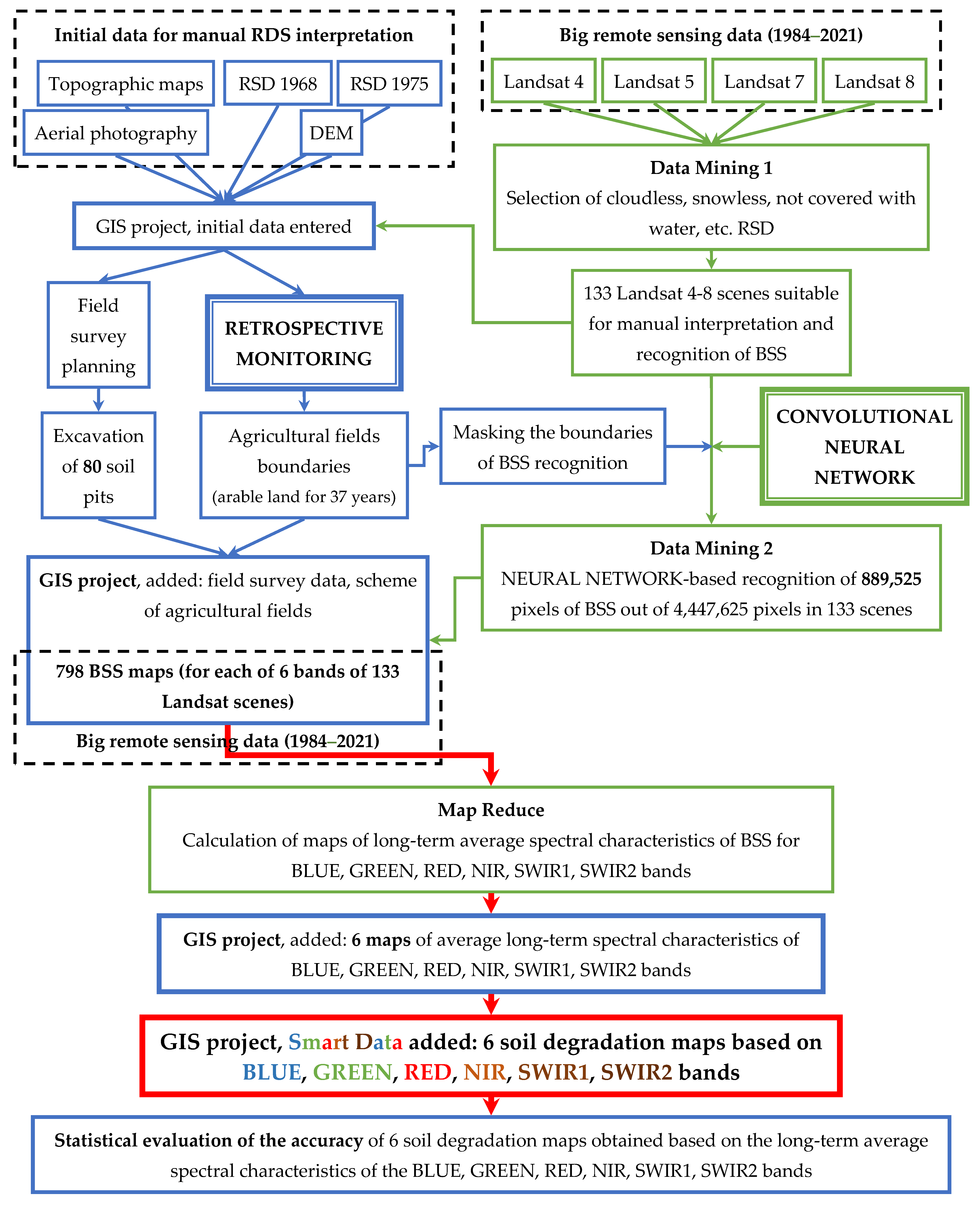
2.1. Flowchart of the Work

This work represents the creation and development of a GIS project for the study area. The flowchart of work is shown on Figure 2. Conventionally, a GIS project is formed in six stages. At the first stage, we do not have any information on the study area, except for the geographical coordinates of the object. All data at this point are in “cloud” storage systems. In the GIS, an extent to search for information is defined. At the second stage, the topographic, space, aerial photographic, and other data from open sources are loaded into the GIS project. The first big data array is formed for the study area. Data mining procedures are used to filter big RSD. At the third stage, as a result of applying the methods of retrospective monitoring of soil and land cover, a convolutional neural network and instructions for organizing a field survey, the GIS project is supplemented with ground data, agricultural field boundaries, and a second array of big RSD (798 BSS maps). The procedure of BSS determining based on a neural network is also an element of data mining.

At the fourth stage, using GIS, the maps of the average long-term characteristics of the BSS in 6 spectral bands are created. The map reduce procedure is carried out; big data convolution. At the fifth stage, based on ground survey data, the maps of long-term average spectral characteristics of BSS are reclassified into maps of soil degradation. From the big data, a smart data was formed. At the sixth stage, statistical methods determine the accuracy of the constructed maps of soil degradation. Thus, the flowchart demonstrates the consistent application of big data processing methods, deep machine learning, and geoinformatics to mapping of soil degradation. The sequential formation of a GIS project in six stages allows the conversion of the big data into smart data through data mining and map reduction procedures using AI.

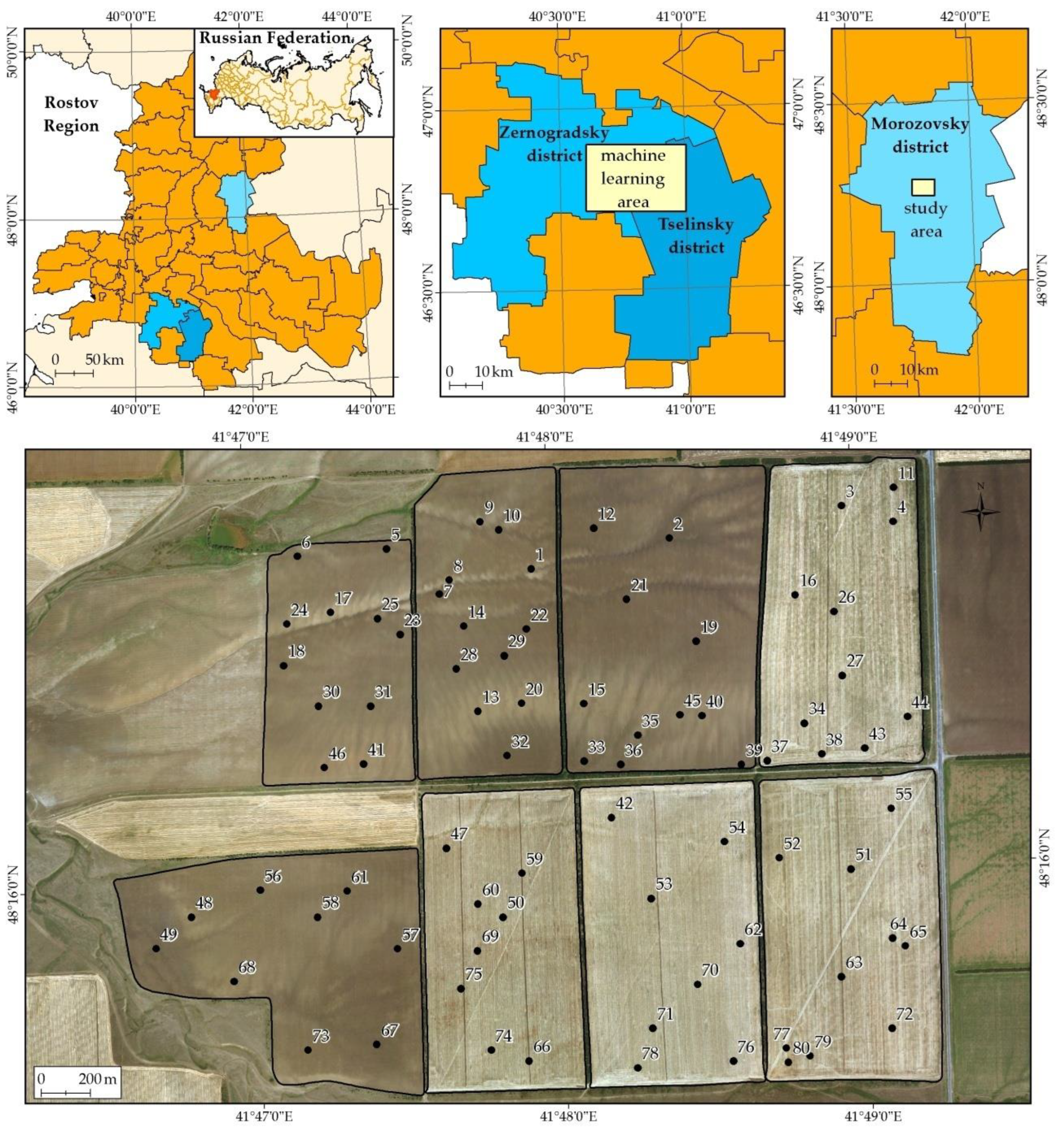
2.2. Retrospective Monitoring of Soil and Land Cover

The method is described in a series of papers of 2013–2020 [35,36,37,38,39]. This method allows the restoration of the change in the boundaries of arable land in the period from the present to 1968. Special detailing of the work is necessary from 1984 to 2021, when there was high dynamics of the areas of arable land in Russia [77]. The method is based on the interpretation of satellite imagery of different spatial resolutions: high spatial resolution (IKONOS, GeoEye-1, WorldView, etc.) [78], medium spatial resolution (Landsat, Sentinel) [79], and archival data from 1968 and 1975 (CORONA) [80]. The accuracy of the method corresponds to the accuracy of traditional mapping at a scale of 1:10,000 [81,82]. The method requires a GIS project of a certain composition and quality.

2.3. GIS Project

A GIS project was created for the study area. It includes the following layers: topographic maps, digital elevation model (DEM) shuttle radar topographic mission (SRTM) 1 arc second [12], remote sensing of high spatial resolution (about 1 m), RSD Landsat 4–8 from 1985 to 2021, and Sentinel-2 space imagery 2016–2021.

All materials used in the work have accurate georeferencing based on large-scale topographic maps. Exact georeferencing was made by local-affine transformations. For aerial photography and the US CORONA mission data, atmospheric correction was not performed. For Landsat and Sentinel, atmospheric correction was carried out using the ATCOR module of the ERDAS imagine software package [83].

When it is possible, the GIS project is supplemented by: ortho-photomaps based on aerial photography, scanned analog space imagery of 1968 with a spatial resolution of 1.8 m (panchromatic, KH-4B satellite, US CORONA mission), scanned analog space imagery of 1975 with a spatial resolution of 6 m (panchromatic, KH-9 satellite, US CORONA mission).

2.4. Deep Machine Learning Flowchart

In the general flowchart of work (Figure 2), a convolutional neural network is used to process big remote sensing data (BRSD); BSS recognition on 133 Landsat 4–8 scenes. Based on the neural network, 798 BSS maps are formed over 37 years. In this case, the convolutional neural network is used to process the acceptance sample, i.e., for processing BRSD that did not participate in deep machine learning. The possibility to apply the results of the neural network (798 BSS maps) for creating of soil degradation maps confirms the correctness of deep machine learning. The acceptance sample is one of the blocks of training the neural network and testing the quality of training (Figure 3). Another block is the processing of the training sample. For training, a dataset is formed from 732 BSS maps (6 bands of 122 Landsat scenes). The dataset is formed by manual determination of the SNSL. Based on the dataset, deep machine learning is carried out. The third block is the test sample. A test sample is formed similarly to the training one, but on a different Landsat path/row. The test sample does not participate in training but is used in the quality control of training.

The training is carried out until the maximum match of the BSS recognition results between the neural network and the test dataset is reached. The trained convolutional neural network is applied in the work, as shown in the general flowchart.

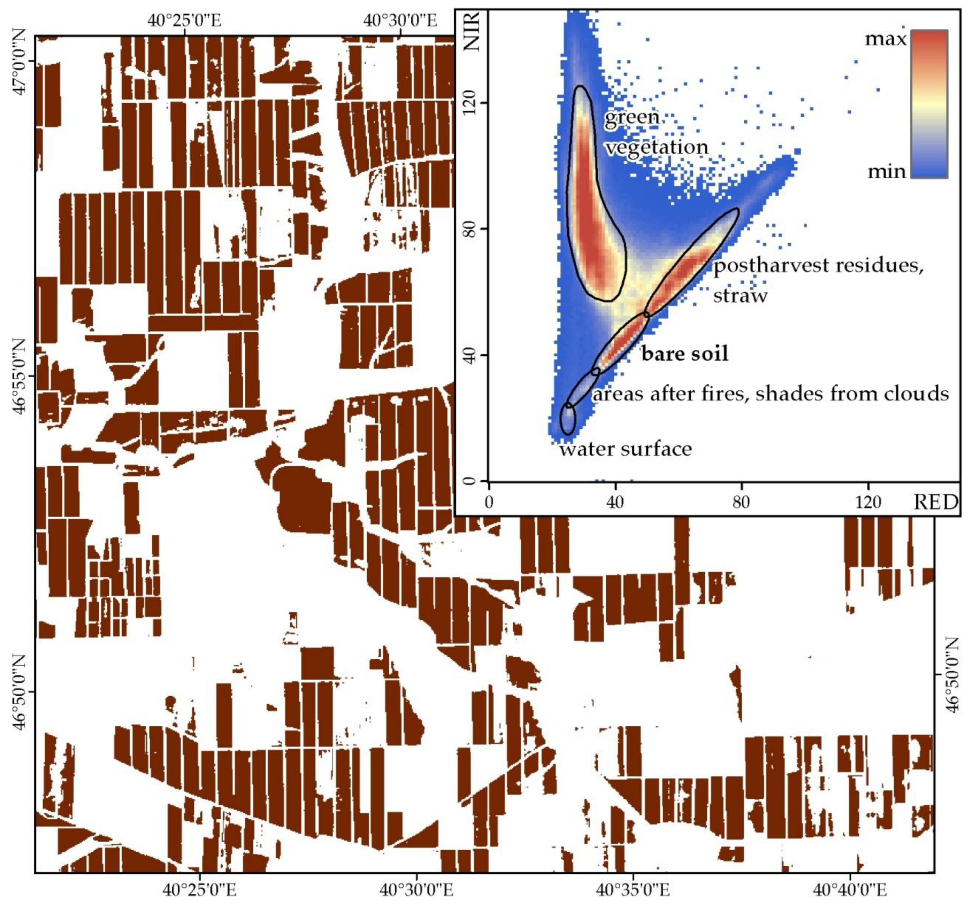
2.5. Identification of BSS on Landsat 4–8 Scenes Based on Deep Machine Learning

The method is described in detail in a 2022 paper [61]. The method consists of training a neural network based on a dataset. The dataset is a series of Landsat scenes from 1984 to 2021, on which bare soil is defined. The BSS on the scenes was highlighted by manually analyzing the RED-NIR (“tasseled cap”) plots of each scene. When selecting, the theory of the spectral neighborhood of the soil line was used. According to this theory, the BSS occupies a specific place on the “tasseled cap” plot (Figure 4).

This area is part of a “tasseled cap” and lies on the soil line [62] between the areas of post harvest residues (straw) and traces of agricultural fires (soot), which are abundant in southern Russia [84]. The location of SNSL only partially coincides with the soil line for VIs of the normalized difference vegetation index (NDVI) type [85]. The trained neural network makes it possible to identify the BSS on any Landsat scenes in similar soil and climatic conditions.

Deep machine learning uses popular neural architecture for image segmentation U-Net [49], the ReLU activation function, batch normalization [86], the Dice Loss function [87], and the Adam optimization algorithm [88].

2.6. Methods for Assessing the Quality of Machine Learning Algorithms

• Test sample. A set of objects not used in learning.
• Acceptance sample. A set of objects not used in development.
• Cross-validation [89,90]. The training sample is divided into N parts and training is performed N times on N-1 parts (without repetitions).

2.7. Calculation of the Average Multi-temporal Spectral Brightness of the BSS in the BLUE, GREEN, RED, NIR, SWIR1 and SWIR2 Bands for Each Landsat Pixel

According to the SNSL technology, the averaged multi-temporal RED-NIR spectral characteristics of the BSS in the form of the average distance of a point with RED-NIR coordinates from the origin of coordinates have information content for constructing soil maps [61]. In this study, the average characteristics of each of the six bands were calculated to identify their informativeness. Only those pixels are considered, where the presence of the BSS is predicted based on the neural network. Thus, “n” is not the total number of Landsat scenes, but the number of Landsat scenes where a pixel is predicted as BSS.

The values of each of the six bands for a pixel are averaged using the formula:

$$BAN{D}_{mean}=\left({\displaystyle \sum }_{i=1}^{n}BAN{D}_i\right)/n$$

Here, BAND—one of the Landsat spectral bands—BLUE, GREEN, RED, NIR, SWIR1 and SWIR2,

BAND_i—band spectral brightness value for the i-th Landsat scene,

i—Landsat scene number in the Landsat scenes database,

n is the total number of Landsat scenes in the Landsat scenes database involved in the calculation of long-term averages,

BAND_mean—average long-term value of the spectral brightness of the band for a pixel,

BAND_mean is calculated for six bands, the result is: BLUE_mean, GREEN_mean, RED_mean, NIR_mean, SWIR1_mean and SWIR2_mean.

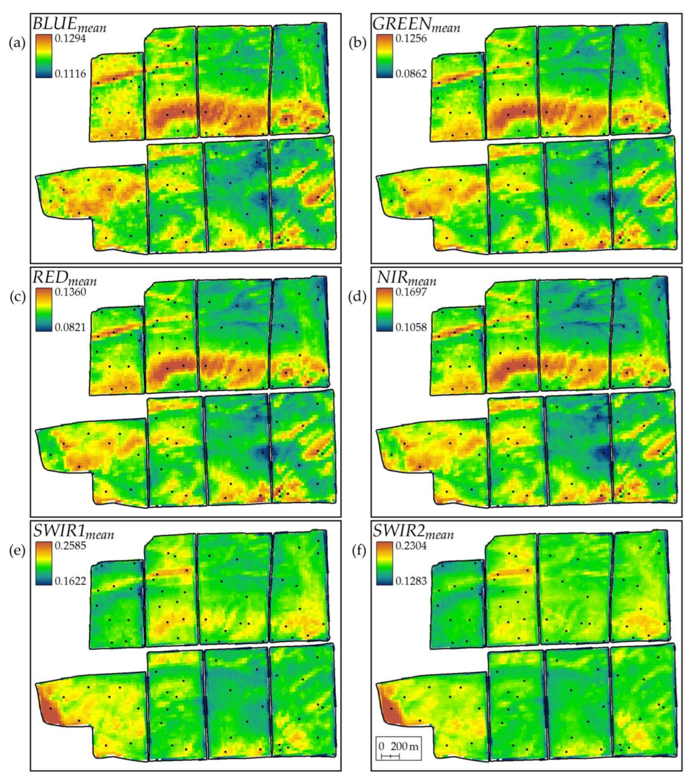
2.8. Mapping of Long-Term Average Spectral Characteristics BLUE_mean, GREEN_mean, RED_mean, NIR_mean, SWIR1_mean and SWIR2_mean for the BSS

The values BLUE_mean, GREEN_mean, RED_mean, NIR_mean, SWIR1_mean and SWIR2_mean were calculated with a spatial resolution of 30 m over the entire study area. Six matrices of values were obtained, which, in raster form, are maps of the distribution of these values.

2.9. Ground Verification

Ground verification was used to check the informativeness and establish the ranges of BLUE_mean, GREEN_mean, RED_mean, NIR_mean, SWIR1_mean and SWIR2_mean values for various soil types/varieties. The soil pits were positioned, and samples were taken by classical methods based on methodological recommendations for field examination [1]. In particular, the soil pits (1.2 m in length, 0.6 m in width) were excavated to a depth of 1 m. Topographic maps and high-resolution RSD were used to determine the locations for ground sampling. On their basis, research routes were determined. At each point with the planned coordinates, a soil pit was excavated. For each soil profile, a description, photographing, and sampling were carried out. The coordinates of the profiles were recorded by a GPS receiver. A soil sample was taken from the top 0–10 cm layer of each profile to measure the organic matter (OM) content. The thickness of the humus horizon was also measured using a tapeline.

The thickness of the humus horizon was understood as the total thickness of the A and AB genetic horizons of the studied soils [91,92,93]. OM content was determined according to Tyurin’s method [94]. A direct analog of Tyurin’s method for determining OM is the Walkley-Black method [95].

Soil type and subtype, as well as the presence of degradation, were determined in the process of describing the soil profiles and using the values of the OM content in the plow horizon and the thickness of the humus horizon. Degradation was understood as a decrease in the thickness of the humus horizon and/or a decrease in the OM content in the plow horizon in relation to the typical soil properties for the study region.

The quality of the interpretation is determined by the percentage of coincidence of degradation definitions in ground surveys, and the calculation of the threshold values of BLUE_mean, GREEN_mean, RED_mean, NIR_mean, SWIR1_mean and SWIR2_mean, characterizing the presence of degradation.

2.10. Cartographic Analysis

Cartographic analysis was performed in AcrGIS [96]. All materials were collected in this GIS. The main method of analysis was the pairwise intersection of different layers of the GIS project. The results of the intersection were recorded in spreadsheets. In electronic tables, the quantitative parameters of the obtained combinations were evaluated, and regression equations were calculated.

3. Results

3.1. GIS Project

A GIS project was assembled for the territory of the Morozovsky district of the Rostov region, including the following layers:

• Topographic maps at a scale of 1:25,000 and 1:50,000;
• Panchromatic aerial photography (2012) with a spatial resolution of 0.6 m (orthophotomap);
• SRTM DEM 1 arc second [12];
• Scanned analogue space imagery of 1968 with a spatial resolution of 1.8 m (panchromatic, KH-4B satellite, US CORONA mission);
• Scanned analogue space imagery of 1975 with a spatial resolution of 6 m (panchromatic, KH-9 satellite, US CORONA mission);
• RSD Landsat 4–8 from 1985 to 2021 (Table S2);
• Space imagery Sentinel-2 of 2016–2021.

3.2. Construction of the Maps of Arable Land Boundaries

Based on the GIS project, the boundaries of arable lands cultivated from 1984 to 2021 were digitized using the method of retrospective monitoring (Figure 1). Eight agricultural fields with a total area of 649 ha have been digitized.

3.3. Ground Surveys

Using classical methods based on layers 1–3 of the GIS project, it was planned to make 80 soil pits (Figure 1). In all soil profiles soil names were determined (meadow chestnut, dark chestnut, dark chestnut slightly eroded, dark chestnut medium eroded, and dark chestnut strongly eroded soils), the thickness of the humus horizon and the OM content in the upper layer of the plow horizon (0–10 cm) were measured. The results of field surveys are presented in

Table 1. Results of ground surveys and BSS long-term average spectral characteristics.

Soil Pit	OM Content, %	Thickness of Humus Horizon, cm	Soil Name *	BLUEmean	GREENmean	NIRmean	REDmean	SWIR1mean	SWIR2mean
1	2.6	31	4	0.12322	0.11048	0.15255	0.11731	0.23055	0.20157
2	3.5	60	1	0.11806	0.09566	0.11650	0.09392	0.19271	0.17115
3	2.7	39	3	0.11921	0.10155	0.13204	0.10375	0.20556	0.18170
4	3.1	53	2	0.11682	0.09614	0.12032	0.09568	0.19569	0.17133
5	2.8	47	2	0.11975	0.09962	0.12763	0.10069	0.19161	0.16462
6	3.0	42	2	0.12075	0.10198	0.13188	0.10298	0.18960	0.16026
7	2.8	36	3	0.11871	0.10083	0.13194	0.10325	0.20385	0.17958
8	2.7	36	3	0.12378	0.10934	0.15006	0.11538	0.22887	0.20096
9	2.3	29	4	0.12429	0.11041	0.15157	0.11735	0.21970	0.18989
10	3.3	47	2	0.11925	0.10174	0.13376	0.10432	0.21079	0.18541
11	3.2	54	1	0.11732	0.09645	0.12112	0.09599	0.19726	0.17455
12	2.8	40	2	0.11910	0.10029	0.12707	0.10206	0.19892	0.17420
13	1.8	27	4	0.12688	0.11854	0.16846	0.13009	0.22646	0.18898
14	3.2	38	3	0.11988	0.10287	0.13276	0.10497	0.19769	0.17123
15	1.8	25	5	0.12706	0.11739	0.16098	0.12738	0.21976	0.18479
16	3.2	56	1	0.11737	0.09626	0.11902	0.09507	0.19256	0.16928
17	1.5	25	5	0.12658	0.11607	0.16174	0.12797	0.21841	0.18214
18	3.1	37	3	0.12025	0.10071	0.12900	0.10273	0.18923	0.16056
19	2.9	39	3	0.11936	0.10165	0.12876	0.10346	0.20496	0.18085
20	1.7	20	5	0.12765	0.11972	0.16917	0.13102	0.22385	0.18655
21	3.4	44	2	0.11875	0.09963	0.12422	0.10046	0.20008	0.17789
22	3.2	42	2	0.11971	0.10322	0.13482	0.10621	0.20838	0.18137
23	3.0	51	2	0.11984	0.10006	0.12688	0.10103	0.18611	0.15863
24	1.9	21	5	0.12527	0.11370	0.15908	0.12406	0.21507	0.18018
25	2.5	37	3	0.12106	0.10280	0.13519	0.10550	0.20142	0.17308
26	3.1	53	2	0.11795	0.09758	0.12395	0.09830	0.20040	0.17803
27	2.1	31	4	0.12343	0.10889	0.14327	0.11466	0.21372	0.18683
28	2.2	35	3	0.12272	0.10734	0.14285	0.11248	0.21182	0.18257
29	2.8	36	3	0.12116	0.10465	0.13770	0.10804	0.20976	0.18295
30	2.2	32	3	0.12146	0.10588	0.14082	0.11151	0.20217	0.17158
31	2.7	41	2	0.12106	0.10501	0.13876	0.11000	0.20324	0.18071
32	3.2	40	2	0.12048	0.10249	0.13196	0.10358	0.20903	0.18603
33	2.8	43	2	0.12120	0.10409	0.13329	0.10659	0.20359	0.17878
34	2.0	23	5	0.12673	0.11711	0.15968	0.12654	0.21991	0.18826
35	2.5	33	3	0.12565	0.11106	0.14683	0.11726	0.21085	0.18223
36	3.0	41	2	0.12055	0.10190	0.12971	0.10170	0.18966	0.16220
37	3.5	52	2	0.12384	0.10233	0.12646	0.10028	0.19003	0.16153
38	3.0	48	2	0.11891	0.10071	0.12953	0.10239	0.20227	0.17828
39	3.0	40	2	0.12139	0.10292	0.13017	0.10173	0.18995	0.16503
40	2.0	25	5	0.12579	0.11447	0.15653	0.12289	0.21564	0.18412
41	2.3	29	4	0.12214	0.10915	0.14799	0.11726	0.20111	0.16700
42	2.7	38	3	0.11907	0.10204	0.13358	0.10527	0.20678	0.18029
43	2.0	22	5	0.12782	0.11830	0.16212	0.12880	0.22545	0.19438
44	2.3	27	4	0.12588	0.11462	0.15761	0.12356	0.21867	0.18481
45	2.0	27	4	0.12543	0.11342	0.15128	0.12130	0.21172	0.18120
46	2.1	25	5	0.12388	0.10975	0.15023	0.11933	0.20418	0.17017
47	3.1	47	2	0.11738	0.10030	0.13191	0.10268	0.19546	0.16632
48	2.1	35	3	0.12313	0.11277	0.15395	0.12115	0.21765	0.18592
49	3.3	53	2	0.12055	0.10150	0.13440	0.10247	0.24074	0.21701
50	2.1	29	4	0.12293	0.10985	0.15179	0.11777	0.21329	0.17967
51	2.3	30	4	0.12460	0.11070	0.14942	0.11729	0.21205	0.18091
52	3.2	46	2	0.11822	0.09909	0.12563	0.10028	0.19229	0.16825
53	3.0	49	2	0.11695	0.09819	0.12518	0.09954	0.19778	0.17147
54	3.5	58	1	0.11527	0.09430	0.11746	0.09472	0.19044	0.16510
55	3.0	42	2	0.11898	0.10097	0.13154	0.10405	0.20315	0.17699
56	2.5	32	3	0.12154	0.10657	0.14102	0.11090	0.21228	0.18359
57	2.5	39	3	0.12060	0.10514	0.13739	0.10873	0.20751	0.17823
58	2.1	26	4	0.12441	0.11099	0.14945	0.11792	0.21410	0.18137
59	2.6	38	3	0.12037	0.10479	0.14125	0.10955	0.20848	0.17821
60	2.3	35	3	0.12129	0.10616	0.14157	0.11068	0.20648	0.17422
61	2.4	39	3	0.12022	0.10556	0.14231	0.10955	0.21603	0.18704
62	3.4	59	1	0.11454	0.09205	0.11157	0.09039	0.18684	0.16652
63	3.3	58	1	0.11693	0.09485	0.11918	0.09421	0.19570	0.17372
64	2.2	30	4	0.12563	0.11249	0.15340	0.12016	0.21781	0.18695
65	3.1	42	2	0.11872	0.10000	0.12723	0.10126	0.19847	0.17298
66	2.0	30	4	0.12388	0.10937	0.15031	0.11647	0.21287	0.17946
67	3.1	44	2	0.11845	0.09909	0.12646	0.09957	0.20740	0.18109
68	2.0	24	5	0.12504	0.11472	0.16003	0.12405	0.22713	0.19562
69	3.3	51	2	0.11925	0.10102	0.13354	0.10466	0.20107	0.17113
70	2.9	45	2	0.11805	0.09958	0.12598	0.10130	0.19548	0.16876
71	2.5	31	4	0.12201	0.10719	0.14240	0.11360	0.20667	0.17784
72	3.3	52	2	0.11688	0.09715	0.12354	0.09731	0.20042	0.17419
73	2.3	32	3	0.12207	0.10702	0.14364	0.11278	0.21713	0.18663
74	2.4	34	3	0.12043	0.10325	0.13968	0.10784	0.20550	0.17455
75	3.1	45	2	0.11815	0.10051	0.13353	0.10397	0.20409	0.17481
76	2.1	22	5	0.12477	0.11389	0.16050	0.12558	0.22699	0.19341
77	1.6	19	5	0.12556	0.11629	0.16574	0.13113	0.21947	0.18349
78	2.4	32	3	0.12321	0.11099	0.15084	0.11861	0.21739	0.18724
79	2.2	24	5	0.12425	0.11186	0.15387	0.12133	0.21454	0.18250
80	3.4	47	2	0.11851	0.10010	0.12998	0.10298	0.19781	0.16864

* Soil names are given in Table 2.

,

Table 2. Classification of ranges of the Landsat bands mean values according to soil varieties.

Soil Number	Soil Name	BLUEmean Range	GREENmean Range	NIRmean Range	REDmean Range
1	Meadow-chestnut	0.114543–0.117373	0.0920461–0.0964505	0.111569–0.121124	0.0903929–0.0959896
2	Dark chestnut	0.117374–0.119842	0.0964506–0.103217	0.121125–0.134816	0.0959897–0.104661
3	Dark chestnut slightly eroded	0.119843–0.123205	0.103218–0.107342	0.134817–0.146825	0.104662–0.112780
4	Dark chestnut medium eroded	0.123206–0.127819	0.107343–0.112491	0.146826–0.153399	0.112781–0.121297
5	Dark chestnut strongly eroded	0.127819–0.127819	0.112492–0.119718	0.153400–0.169174	0.121298–0.131129

and Table S3 and as a GIS layer in *.shp format (Figure 1).

The average OM content for dark chestnut soils in this study is 3.1%, which is in significant agreement with the characteristics of this zonal soil—dark chestnut slightly solonetzic clayey and heavy loamy soils on loess-like clays and loams [91]. This soil variety is characterized by the following values: the thickness of the humus horizon is 40–60 cm and the content of OM is 3–4% [92]. The threshold values of the OM content and the thickness of the humus horizon (2.7% and 40 cm), as characteristics of degradation, were also determined during the field survey based on the typical characteristics of soil types and subtypes in the study area.

3.4. Construction of BSS Masks

The dataset for the neural network was compiled based on 244 Landsat scenes for two path/row—173/028 and 174/027 [61]. For each Landsat scene, a mask of the BSS was built on the principles of SLNS [29,30,31,32,33] (Figure 4). A total of 567,127,808 learning elements were used, of which 112,632,627 are BSS. Half of the dataset (122 Landsat scenes 173/028) was used as a training sample with cross-validation. The second half of the Landsat scenes (174/027) was used as a test sample. The total IoU estimate (the intersection over union between the predicted and the corresponding manually constructed bare soil masks) of the proposed model on the validation set is 0.79.

The territory of the study region was used as an acceptance sample. On 551 Landsat 173/026 scenes, based on deep machine learning, the BSS was observed, 133 Landsat scenes from 1 April 1985 to 30 November 2021 were selected for calculations. The BSS was predicted 889,525 times and 133 BSS masks were created.

3.5. Maps of Long-Term Average Spectral Characteristics BLUE_mean, GREEN_mean, RED_mean, NIR_mean, SWIR1_mean and SWIR2_mean for BSS

Using the BSS masks for 133 Landsat scenes for each of the 6 spectral bands, the calculation of the long-term average values of the spectral brightness for the period from 1985 to 2021 was carried out. The calculation results are shown in Figure 5. To facilitate visual analysis, the maps are presented in the uniform palette, but based on each band’s own histogram.

3.6. Additions to the GIS Project

The following layers were added to the GIS project:

8.

Layer of ground survey results;

8.1

The content of OM in a layer of 0–10 cm;

8.2

Thickness of the humus horizon;

8.3

Names of soil varieties;

9.

Maps of long-term average spectral characteristics BLUE_mean, GREEN_mean, RED_mean, NIR_mean, SWIR1_mean and SWIR2_mean for BSS.

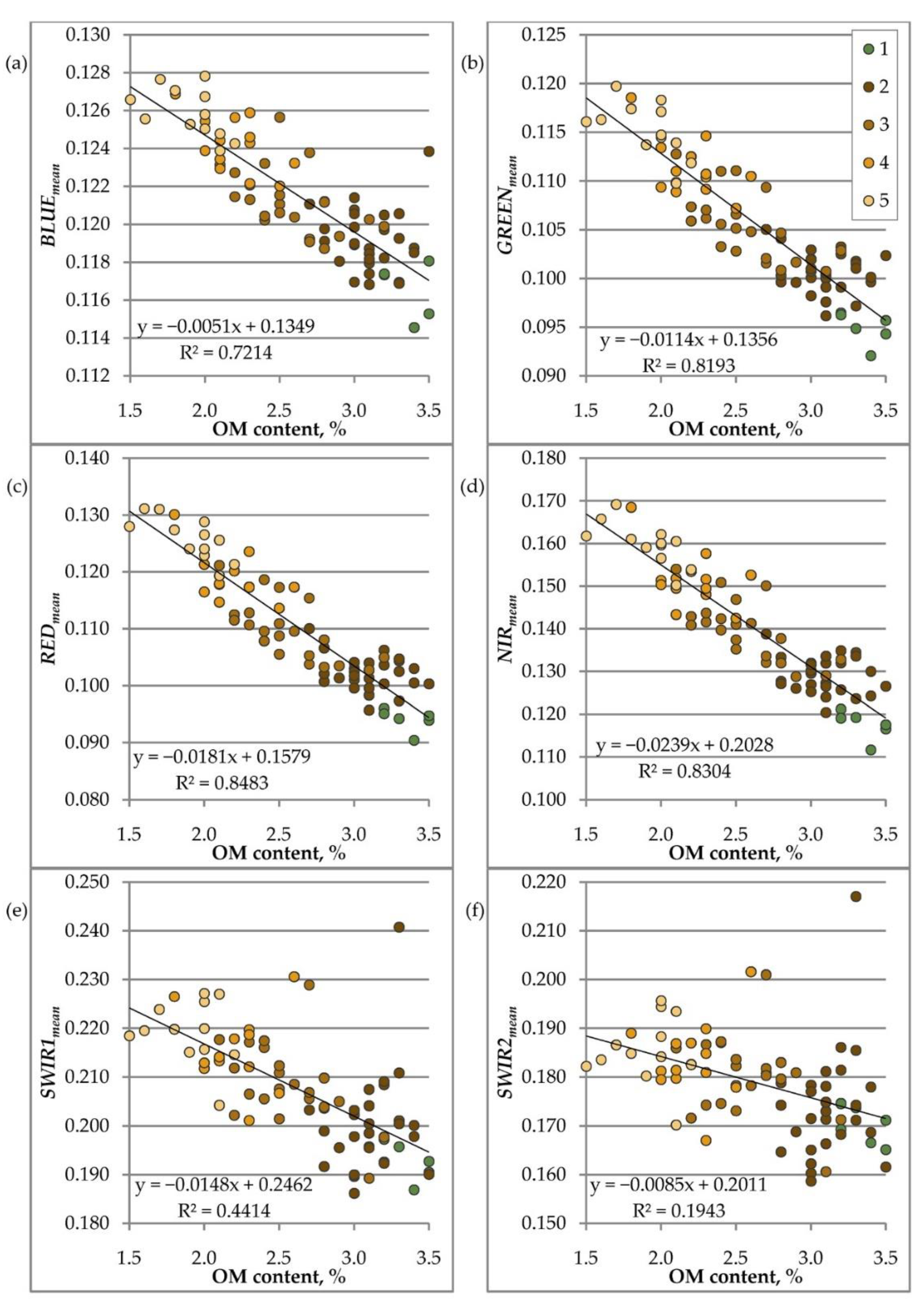
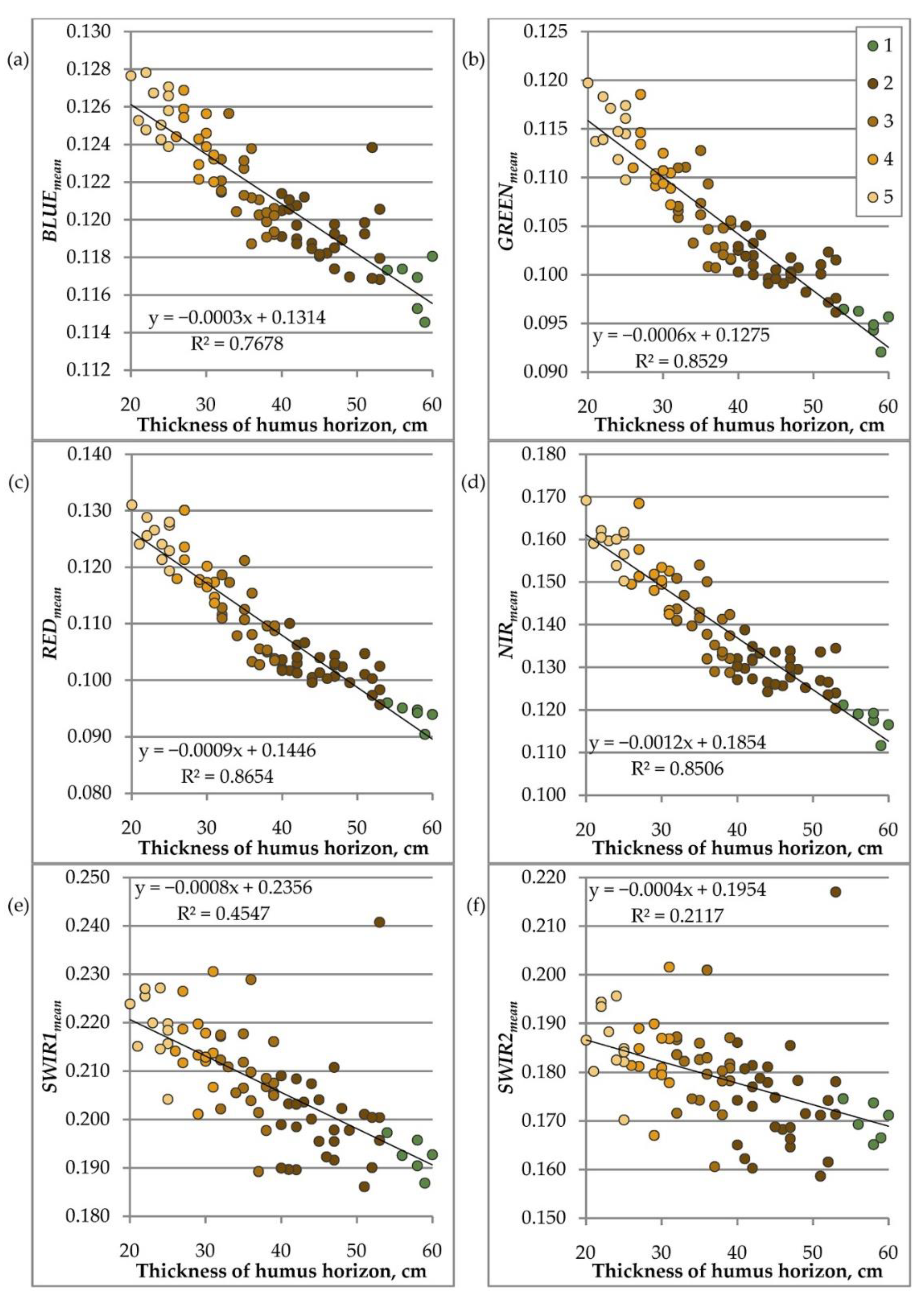
3.7. The Intersection of the Results of Ground Surveys and Maps of Average Long-Term Spectral Characteristics of the BSS

GIS project layers 8.1 and 8.2 were intersected with 6 maps of mean long-term spectral characteristics. The results are presented in Table 1 and Table S2. A graphical representation of the dependences of the long-term average spectral brightness of 6 Landsat bands on the OM content in the 0–10 cm layer and the thickness of the humus horizon is shown on the graphs (Figure 6 and Figure 7). The graphs also show the results of the regression analysis.

The quality of the regression model decreases in the following sequence of spectral bands: RED_mean, NIR_mean, GREEN_mean, BLUE_mean, SWIR1_mean, and SWIR2_mean. The high values of the R² coefficient (0.721–0.848) make it possible to interpret the maps of the long-term average spectral characteristics RED_mean, NIR_mean, GREEN_mean, and BLUE_mean as maps of the OM content in the plow horizon. The low values of R² (0.194–0.441) SWIR1_mean and SWIR2_mean show that these bands cannot be used for mapping the OM content. Similarly, the R² values characterize the possibility of constructing maps of the thickness of the humus horizon using RED_mean, NIR_mean, GREEN_mean, and BLUE_mean and the impossibility of constructing maps using SWIR1_mean and SWIR2_mean.

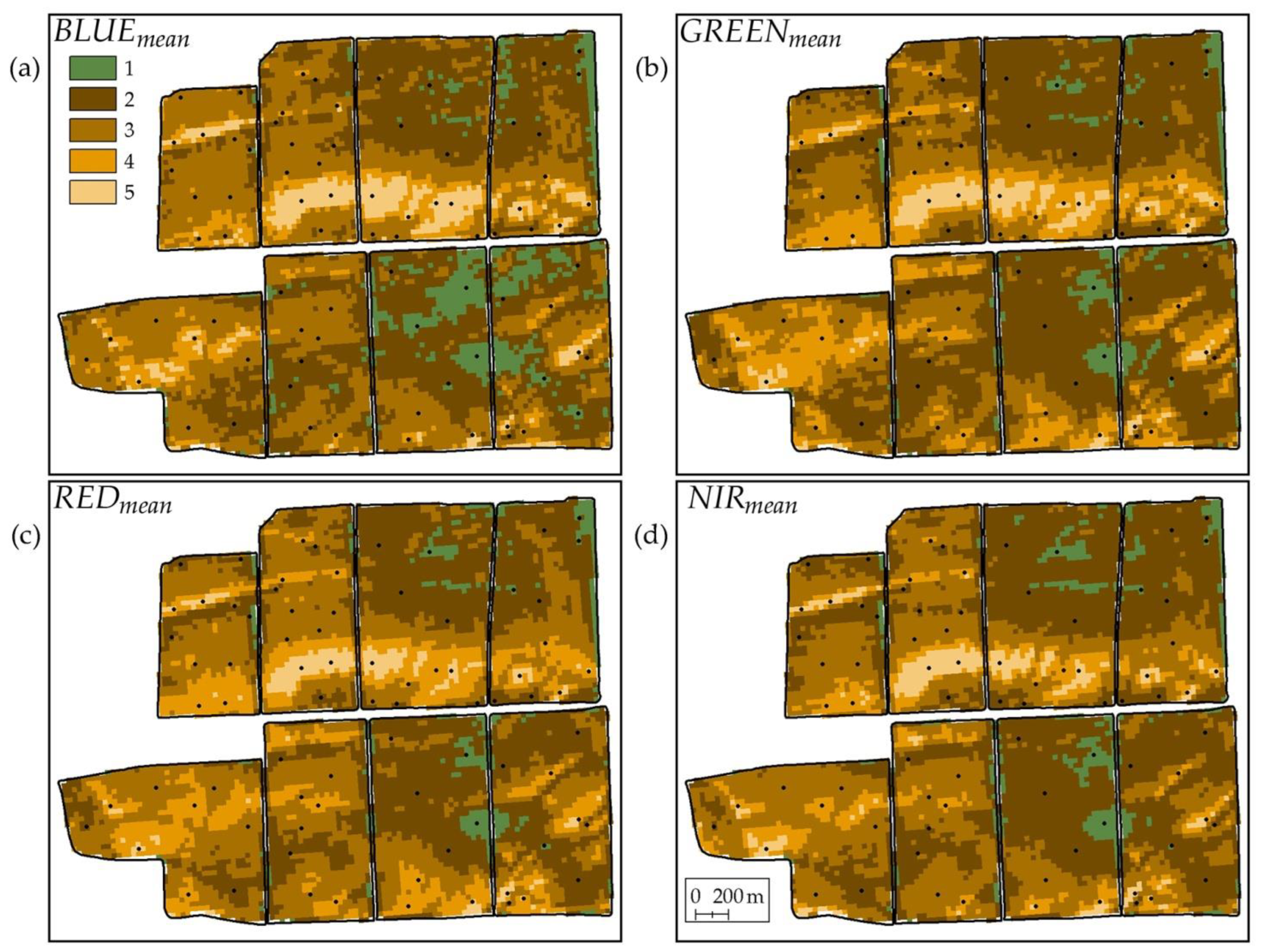
3.8. Soil Interpretation of Maps of BSS Long-Term Average Spectral Characteristics

During ground surveys, 5 soil varieties were described for 80 soil profiles: meadow-chestnut, dark chestnut, dark chestnut slightly eroded, dark chestnut medium eroded, and dark chestnut strongly eroded soils.

For each of 80 profiles, the RED_mean, NIR_mean, GREEN_mean, BLUE_mean, SWIR1_mean, and SWIR2_mean values were obtained. Analysis of variance (ANOVA) and a post hoc analysis of the significance of differences in the spectral characteristics of soil varieties in each spectral band were carried out (Tables S4–S10). For the RED, NIR, and GREEN bands, all five soil varieties differ significantly in long-term average spectral characteristics. For the BLUE band, strongly and moderately eroded soils are spectrally indistinguishable. For the SWIR1 band, 3 out of 10 possible pairs of soils are spectrally indistinguishable. For the SWIR2 band, 8 out of 10 possible soil pairs are spectrally indistinguishable. For the SWIR1 and SWIR2 bands, none of the five soil varieties can be statistically significantly separated from the remaining 4 soil varieties. Based on the statistical analysis performed, it can be assumed that soil maps can be constructed based on the long-term average spectral values for the RED, NIR, GREEN, and BLUE bands. SWIR1 and SWIR2 bands are not suitable for soil interpretation.

Based on the soil types/names for 80 profiles, the ranges of long-term average brightness values were empirically selected for each of the four (RED, NIR, GREEN, and BLUE) Landsat bands for each soil variety (Table 2). Soil interpretations of mean long-term spectral brightnesses for four bands are presented on Figure 8 and added as layer 10 in the form of four soil maps in the GIS project.

The accuracy of the soil maps can be estimated by the number of soil profiles correctly interpreted by spectral characteristics (

Table 3. Type I and II errors for soil varieties identification.

Soil Name	Total Number of Soil Pits in the Corresponding Interval of Mean Band Values	Properly Defined Soil Varieties		Type I Errors (False Positive)		Type II Errors (False Negative)
		(Soil Pits Number)	%	(Soil Pits Number)	%	(Soil Pits Number)	%
BLUE band
1. Meadow-chestnut	8	5	62.5	3	37.5	1	12.5
2. Dark chestnut	22	17	77.3	5	22.7	10	45.5
3. Dark chestnut slightly eroded	25	15	60.0	10	40.0	5	20.0
4. Dark chestnut medium eroded	10	6	60.0	4	40.0	7	70.0
5. Dark chestnut strongly eroded	15	10	66.7	5	33.3	2	13.3
GREEN band
1. Meadow-chestnut	7	6	85.7	1	14.3	0	0.0
2. Dark chestnut	32	25	78.1	7	21.9	3	9.4
3. Dark chestnut slightly eroded	13	10	76.9	3	23.1	11	84.6
4. Dark chestnut medium eroded	16	10	62.5	6	37.5	3	18.8
5. Dark chestnut strongly eroded	12	10	83.3	2	16.7	2	16.7
RED band
1. Meadow-chestnut	7	6	85.7	1	14.3	0	0.0
2. Dark chestnut	28	24	85.7	4	14.3	4	14.3
3. Dark chestnut slightly eroded	16	13	81.3	3	18.8	8	50.0
4. Dark chestnut medium eroded	16	11	68.8	5	31.3	2	12.5
5. Dark chestnut strongly eroded	13	11	84.6	2	15.4	1	7.7
NIR band
1. Meadow-chestnut	7	6	85.7	1	14.3	0	0.0
2. Dark chestnut	32	26	81.3	6	18.8	2	6.3
3. Dark chestnut slightly eroded	15	12	80.0	3	20.0	9	60.0
4. Dark chestnut medium eroded	12	9	75.0	3	25.0	4	33.3
5. Dark chestnut strongly eroded	14	11	78.6	3	21.4	1	7.1

). For the RED band, 81.3% of soil profiles were correctly determined; for the NIR band—80.0%; for the GREEN band—76.2; and for the BLUE band—66.3%.

The accuracy of the thematic interpretation of the long-term average spectral characteristics of the four Landsat bands calculated from big satellite data can be analyzed in terms of information theory. It is possible to set the values of errors of the I and II type for five soil varieties. According to information theory, we have type I errors—false positive and type II errors—false negative. False positive errors in this study mean that another soil variety fell within the range of spectral characteristics (Table 2) for one soil variety. False negative errors mean that the soil variety did not fall within the range of spectral values selected for it. Errors of the I and II types for the spectral bands for soil varieties are summarized in Table 3. It follows from the table that both false positive and false negative errors differ for different soils and bands. False positive errors range from 14.3% to 40.0%, false negative—from 0% to 84.6%. The maximum contribution to the errors is made by slightly eroded and moderately eroded dark chestnut soils, which have similar spectral characteristics. Overall, according to the soil maps of the ranges of long-term average spectral characteristics for four bands, out of 80 sections from 53 to 65 profiles fell into their legend classes (ranges of values) (Table 3). Thus, the overall accuracy of the four soil maps ranges from 66.3% to 81.3%.

The results of the ANOVA showed that the classification of the long-term average spectral characteristics of the four Landsat bands by soil varieties is statistically significant, both by the OM content and the thickness of the humus horizon (Tables S11–S12).

A post hoc analysis of the means according to the Tukey test (Tables S13–S16) showed that by the OM content in the 0–10 cm layer, meadow-chestnut and dark chestnut soils, as well as slightly and moderately eroded dark chestnut soils, do not differ from each other for the BLUE, NIR and GREEN bands. For the RED band, only meadow chestnut and dark chestnut soils do not differ in OM content.

According to the Tukey criterion (Tables S17–S20), all soil varieties of the constructed soil maps differ by the thickness of the humus horizon, for the RED, NIR, GREEN bands. For the BLUE band, slightly and moderately eroded soils do not differ by the thickness of the humus horizon.

Most soil varieties in soil maps created using four bands (RED, NIR, GREEN, and BLUE) long-term average values, differ statistically significantly from each other by thickness of the humus horizon, and OM content in the 0–10 cm layer.

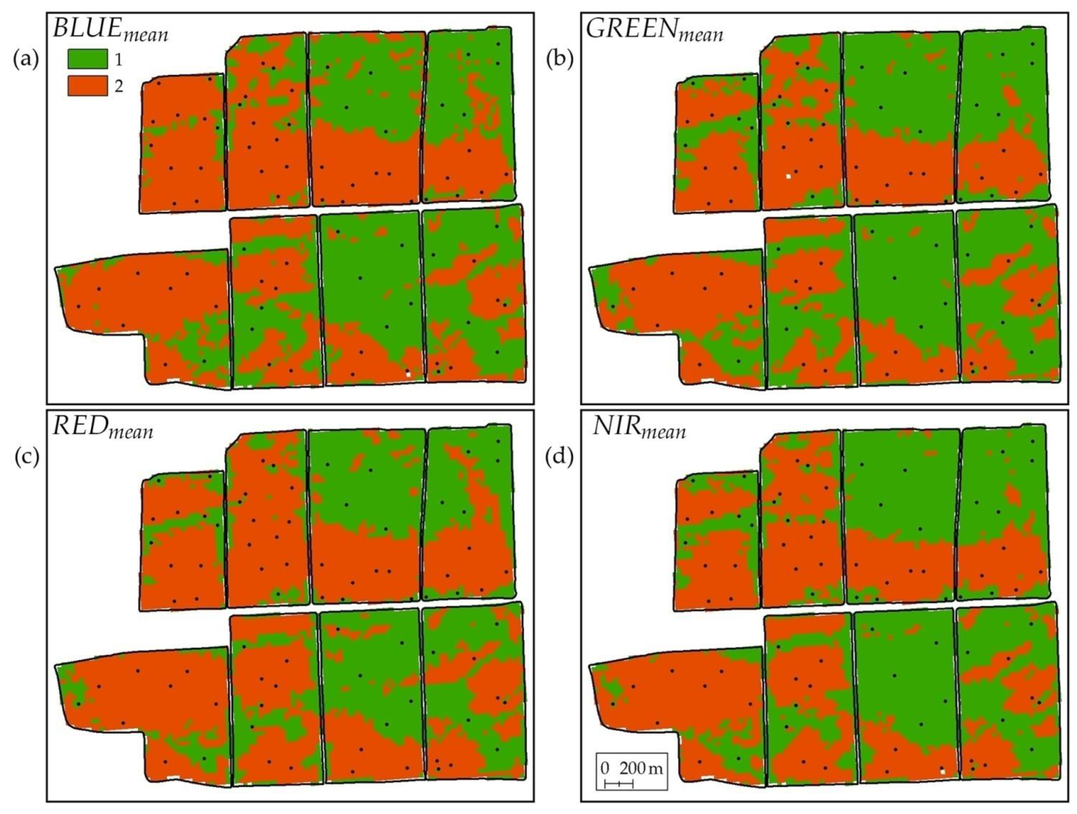
3.9. Construction and Ground Verification of Degradation Distribution Maps

Three of the five soil varieties identified during the field study are classified as degraded soils, i.e., soils slightly, moderately and strongly eroded. Degraded soils differ from the dark chestnut soils of this region by a smaller thickness of the humus horizon and a lower content of OM in the upper layer of 0–10 cm. For dark chestnut soils, the thickness of the humus horizon should be 40–60 cm with the OM content in the layer of 0–10 cm from 3% to 4% [97,98]. Meadow-chestnut soils have a greater thickness of the humus horizon and a higher content of OM. Therefore, a decrease in the thickness of the humus horizon of less than 40 cm or a decrease in the OM content of less than 3% can be interpreted as a soil degradation. In this work, the threshold of OM content for determining degradation was 2.7%. Out of 80 soil profiles, 46 belong to degraded soils and 34 to non-degraded soils.

Four degradation distribution maps (Figure 9) were created by grouping degraded and non-degraded soil differences of maps of soil interpretation of multi-temporal spectral characteristics. The spectral ranges are given in

Table 4. Classification of ranges of the Landsat bands mean values according to soil degradation.

Band	Non-Degraded Soils	Degraded Soils
BLUE	0.114543–0.119842	0.119843–0.127819
GREEN	0.0920461–0.103217	0.103218–0.119718
NIR	0.111569–0.134816	0.134817–0.169174
RED	0.0903929–0.104661	0.104662–0.131129
SWIR1	0.186105–0.204092	0.204093–0.240738
SWIR2	0.158627–0.178033	0.178034–0.217006

. As a result of the intersection of the layer of soil profiles (layers 8.1 and 8.2) with maps of the distribution of degradation,

Table 5. Type I and II errors for soil degradation identification.

Band	Degraded Soils Based on BANDmean Value (Soil Pits Number)	Non-Degraded Soils Based on BANDmean Value (Soil Pits Number)	Type I Errors (False Positive)		Type II Errors (False Negative)		Total Error, %
			(Soil Pits Number)	%	(Soil Pits Number)	%
BLUE	30	50	7	14.0	4	8.0	22.0
GREEN	39	41	2	4.9	7	17.1	22.0
NIR	39	41	1	2.4	6	14.6	17.1
RED	35	45	3	6.7	4	8.9	15.6
SWIR1	35	45	5	11.1	6	13.3	24.4
SWIR2	35	45	8	17.8	9	20.0	37.8

was obtained. The false negative errors of degradation maps vary from one spectral band to another from 8% to 17%. False positive errors range from 2.4% to 14%. The overall degradation prediction accuracy ranges from 78.0% to 84.4%. The accuracy of soil degradation maps was determined as the percentage of soil profiles that fell outside their degradation class according to spectral classification, out of the total number of soil profiles that fell into the spectral brightness range determined as the area of soil degradation.

ANOVA showed that although the soil differences for the SWIR1 and SWIR2 bands are indistinguishable, the spectral brightnesses for degraded and non-degraded soils differ significantly (Table S21). Therefore, it is possible to construct maps of soil degradation bypassing the stage of constructing maps of soil interpretation of spectral characteristics. Soil degradation maps constructed for the SWIR1 and SWIR2 bands are shown in Figure 10. The ranges of spectral values for the SWIR1 and SWIR2 bands are given in Table 4. The degradation prediction accuracy was 75.5% and 62.2%. The results of the ANOVA showed that the classification of the long-term average spectral characteristics of the six Landsat bands for soil degradation is statistically significant both by OM content and the thickness of the humus horizon (Tables S22 and S23).

4. Discussion

4.1. Analysis of the Soil Interpretation of the Maps of the Long-Term Average Spectral Characteristics BLUE_mean, GREEN_mean, RED_mean, NIR_mean, SWIR1_mean, and SWIR2_mean for the BSS

Six Landsat spectral bands showed different informativeness for the construction of soil and soil degradation maps. In descending order of informativeness for soil mapping, the bands are arranged in the following order: RED, NIR, GREEN, BLUE, SWIR1, SWIR2. The first four bands can be used to construct soil maps with an accuracy from 81.3% (RED) to 66.3% (BLUE). The last two bands cannot be used to construct soil maps. The RED and NIR bands are close in information content (80.0%). Using the same 4 bands, it is possible to create binary degradation maps with even higher accuracy from 84.4% (RED) to 78.0% (BLUE). This confirms the correctness of the choice of RED-NIR bands, which are used to calculate VIs, for constructing soil maps based on the analysis of the BSS [61]. On the other hand, to create degradation maps with an accuracy of at least 78.0%, possible to use any of the 4 bands: RED, NIR, GREEN, BLUE. That is, the presence of an infrared band is not strictly necessary for the construction of soil degradation maps, the visible range is sufficient. Moreover, with an accuracy of 75.5% and 62.2%, soil degradation maps can also be constructed using the SWIR1 and SWIR2 bands.

It should be assumed that the spectral reflectivity of the soil increases with a decrease of OM content almost identically in four of the six Landsat bands, what can be clearly seen in the graphs of Figure 6. Soil varieties significantly differ in the content of OM in the soil layer of 0–10 cm, which makes possible the soil mapping. The relatively low accuracy of the soil interpretation of the map of mean long-term values for the BLUE band can be explained by the small range of values for this band (Table 2). The long-term average spectral values for the RED band vary from 0.090 spectral units to 0.131. While for the BLUE band, the range is from 0.114 to 0.127. With the same spectral discretization of the Landsat bands, the BLUE band simply has fewer possible values, which makes it difficult to set the spectral ranges for soil mapping. Perhaps this explains the relatively low accuracy of soil interpretation for 5 soil varieties (66.3%). To create a binary map of soil degradation, the spectral range of the BLUE band is quite sufficient to achieve an accuracy of 78.0%.

The situation is more complicated for bands SWIR1 and SWIR2. The content of OM affects the spectral brightness of both bands, but the relationship is much weaker—R² = 0.19–0.44. It was noted that in the floodplain positions, the reflectivity in the bands SWIR1 and SWIR2 increases even with an increased content of OM (point 49, Figure 1). According to a post hoc analysis in the SWIR1 and SWIR2 bands, only non-degraded soils can be distinguished from highly degraded ones (Tables S9 and S10). Thus, if it is necessary, to detect strong degradation, could be used the SWIR1 and SWIR2 bands. But for soil mapping, the information content of these bands is insufficient.

The RED band has the maximum information content in soil mapping.

4.2. Analysis of the I and II Type Errors of Degradation Maps Constructed by Reclassifying Maps of Soil Interpretations of Multi-Temporal Spectral Characteristics

4.2.1. BLUE Band

False negative errors were noted 4 times. In all cases, the OM content was 2.7–2.9% which is close to the degradation detection threshold of 2.7%. Degradation was determined only by the thickness of the humus horizon—36–39 cm. False positive error occurred in 7 cases with OM content of 2.7–3.2% and a thickness of the humus horizon of 40–53 cm. Errors of the first and second type confirm the relatively low correlation between the long-term average brightness characteristics of the band and the OM content—R² = 0.72. But it should be noted that errors occur at the degradation threshold of 2.7% OM content, which is explained by the small spectral range of the BLUE band values. There are not enough values to accurately determine the spectral threshold for detecting degradation.

The BLUE band gives the maximum number of errors of the first type—a false positive.

4.2.2. GREEN Band

False negative errors were noted 7 times. In 6 cases, the OM content was higher or equal to 2.7%. Degradation was recorded only by a decrease in the thickness of the humus horizon below 40 cm. False positive errors occurred 2 times. In both cases, the OM content was at the degradation detection threshold. The presence of errors of the I and II type is due to the complexity of setting the spectral threshold to determine soil degradation. Despite the higher correlation between the long-term average brightness values of the GREEN band (R² = 0.81) compared to the BLUE band, the total error of both maps is 22%.

When soil degradation is detected by the GREEN band, the degradation area is underestimated. The band gives the maximum number of errors of the II type false negatives. Difficulties are noted with the determination of the brightness threshold for determining degradation.

For the GREEN band, there is a single point that refers to degraded soils by both parameters (thickness of humus-accumulative horizon and OM content) but is not detected by brightness as degradation. In other bands, this phenomenon is not observed. An explanation for this was not found in this work.

4.2.3. RED Band

False negatives were recorded 4 times. In all cases, the OM content is above or equal to the degradation threshold. In all cases, degradation was determined only by the thickness of the humus horizon—36–39 cm. False positive errors were recorded 2 times. The RED band analysis achieved the maximum accuracy of soil cover degradation detection of 84.6%.

4.2.4. NIR Band

False negative errors were marked 6 times. In all cases, the OM content exceeded or was equal to the threshold of 2.7%. Degradation was determined only by the thickness of the humus horizon—38–39 cm. Degradation can be detected very accurately using the NIR band, since an error of the II type occurs when ground-based measurements are close to the threshold values. A false positive error also occurs at a point with near-threshold values—2.7% OM and 41 cm thickness of the humus horizon.

The NIR band has the lowest false positive error—1 case.

Note that there are 3 points (soil profiles), which give an error of the II type (false negative) for all 4 bands. These points are in transit landscape positions and belong to weakly eroded soils. The thickness of the humus horizon in these soils is below 40 cm, but the OM content is above 2.7%. The OM content in these soils is supported by sediment delivery from higher landscape positions. It can be assumed that the soils are eroded and sediment-accumulated, which ensures a relatively high content of OM at a relatively low thickness of the humus horizon. Obviously, it is these landscape positions that will determine the upper threshold of accuracy of the proposed mapping method based on long-term average spectral characteristics.

The minimum errors in the creation of degradation maps were achieved when analyzing the RED band.

4.3. Analysis of the I and II Type Errors of Degradation Maps Constructed by Direct Classification of Multi-Temporal Spectral Characteristics

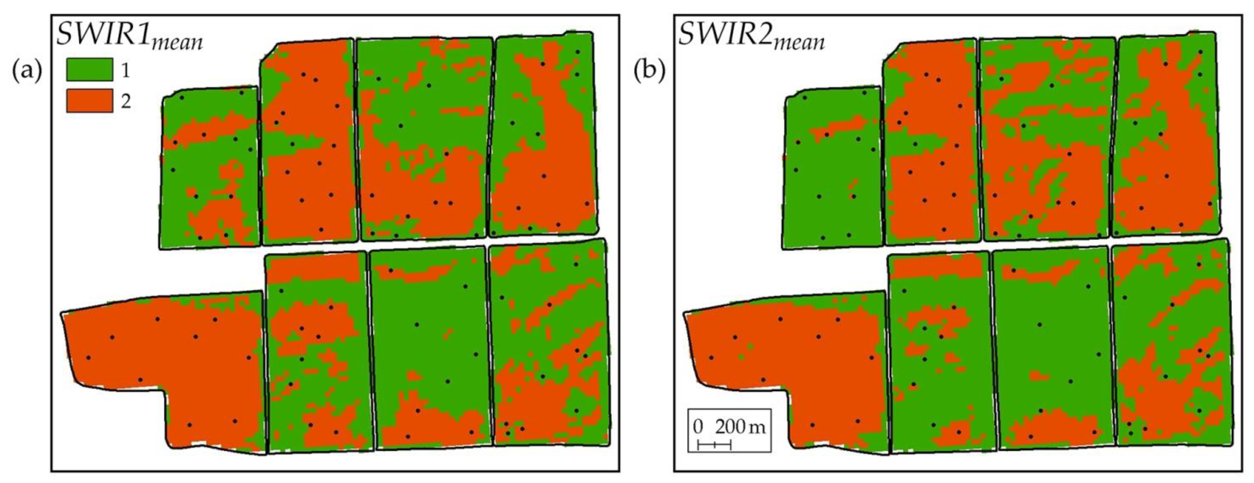
For the RED, NIR, GREEN, and BLUE bands, soil cover degradation maps were built based on previously constructed soil maps. For SWIR1 and SWIR2 bands, degradation maps were constructed by direct division of the band spectral range into two classes. The errors of these groups of maps differ from each other.

4.3.1. SWIR1 Band

False negative errors for the band occurred 6 times. Of the 6 times, 3 times points were missed, where soil degradation was recorded both by the OM content and the thickness of the humus horizon. For false positive errors, all 5 cases refer to non-degraded soils by both parameters. Twice with a false positive error, the OM content is 3.3%, which is not typical for the first 4 spectral bands.

4.3.2. SWIR2 Band

False negative errors were marked 9 times. Soil profiles where degradation by ground methods was recorded both by OM content and thickness were skipped five times. False positive errors were recorded 7 times. As for the SWIR1 band, in all cases these are non-degraded soils by both parameters.

The main difference between the degradation maps for the SWIR1 and SWIR2 bands and the RED, NIR, GREEN and BLUE bands is that the errors of both types are not close to the specified degradation thresholds. That is, a false positive error can occur when the thickness of the humus horizon is 53 cm, and the OM content is 3.3%. The errors for the SWIR1 and SWIR2 bands look illogical in terms of the effect of degradation on the spectral brightness. The errors for these two bands are not the same as those for the RED, NIR, GREEN, and BLUE bands. No additional factors affecting the spectral values of the SWIR1 and SWIR2 bands were identified in this study.

4.4. Physical Interpretation of Work Technology

This study was based on the assumption that the brightness characteristics of the soil cover are related to the OM content in the topsoil layers. It was assumed that in each satellite image, the spectral characteristics of the soil moisture and the agrotechnical/tillage methods of its processing affect the spectral characteristics of the soil. During long-term observations, it was assumed that most of the RSD pixels would go through different stages of wetting and different agrotechnical treatments. As a result, dozens of spectral states of a pixel will be accumulated over 35 years, in which the influence of different soil humidity of each date of acquisition of the satellite image will be mutually leveled. That is, the number of wet states of a pixel is offset by the number of dry states. As a result, long-term average data will reflect more inert factors affecting soil reflectivity. Similarly, agrotechnical methods will have to undergo mutual compensation, since in principle these methods are the same for all fields during the crop rotation. For 35 years, several crop rotations had to change.

This hypothesis was tested when constructing a soil map based on the principles of the spectral neighborhood of the soil line [61]. Indeed, in the RED-NIR spectral space, the BSS occupies a specific place in the form of an ellipse of possible values over decades [32]. With an increase in humidity, the image of the soil darkened, and the spectral reflectivity decreased. With a decrease in humidity, the opposite process was observed. Of the three independent factors affecting the spectral reflectivity (OM content, humidity, agricultural practices), only the OM content was long-term stable.

When analyzing the RED and NIR bands independently, these assumptions were confirmed. Indeed, the average long-term characteristics of the bands for the BSS have a high correlation with the OM content in the 0–10 cm layer. The assumptions about the predominant effect of the OM content on the spectral reflectivity for the BLUE and GREEN bands were also confirmed. In fact, all four (RED, NIR, GREEN, BLUE) Landsat bands behave in the same way in terms of OM content, moisture level and farming practices. The brightness of the soil in these bands decreases with an increase in the OM content, an increase in moisture, and loosening of the plow horizon. It can be assumed, that when loosening (plowing, harrowing, disking) the arable horizon, the soil comes to the surface in a wetter state. With a decrease in the OM content, in moisture, and the formation of a dry soil crust, the reflectivity of the BSS increases.

It was also confirmed that data for 35 years allow, due to big data, to mutually compensate the influence of humidity and agricultural practices. The OM content in the upper arable horizons becomes a main factor affecting the spectral reflectivity.

For bands SWIR1 and SWIR2 the situation is somewhat different. It can be argued that the SWIR1 and SWIR2 bands are influenced by factors not related to OM content, moisture and agricultural practices. The available ground data did not allow to establish these factors. It was only noted that in several landscape positions (floodplain terraces) in the SWIR1 and SWIR2 bands, the spectral brightness increases with an increase of the OM content. This effect sharply distinguishes the SWIR1 and SWIR2 bands from the RED, NIR, GREEN, BLUE bands.

Of course, moisture and OM content are not the only factors affecting the reflectivity of soils. Parent material and soil texture have a great influence. But within the study area, the soils are formed on a single parent rock and have the same type of granulometric composition, which makes it possible to exclude their impact. Increased reflectivity is also an indicator of non-compliance with the rules of soil use, which leads to an increase in losses due to erosion and, as a result, a decrease in the content of OM [99].

This is the physical interpretation of the work; the need for interpretation is substantiated in [100]. As a physical interpretation, regression models of calculated parameters and field measurements were used [101,102].

4.5. Perspective RSD and Direction of Work

The work [61] showed the possibility of constructing soil degradation maps based on the average long-term characteristics of the RED-NIR bands. This study shows that, in practice, a soil degradation map can be built using the average long-term characteristics of any of the 5 spectral bands (RED, NIR, GREEN, BLUE, SWIR1) with an accuracy of at least 75.0%. It is important that it is enough to use only the bands of the visible range, without the analysis of infrared bands. There are more options for RSD in the visible range than Landsat analogues.

But the previous and current work is based on BSS recognition using all 6 bands—RED, NIR, GREEN, BLUE, SWIR1 and SWIR2. We have not studied the issue of reducing the number of spectral bands when training a neural network to recognize BSS with acceptable accuracy. In the future, this issue needs to be studied in more detail. If a smaller number of spectral bands are sufficient for BSS recognition, then this can expand the number of RSD sources for constructing soil degradation maps based on big satellite data.

The second question that remains open is to what extent the reduction in the time range of satellite imagery used affects the accuracy of soil degradation mapping. At this stage of the work, the maximum time series of the same type of RSD with the same spatial and spectral calibration were used—Landsat 4–8 data for 37 years. This issue is more relevant since the Sentinel 2A,B archive is being formed. The temporal coverage of this archive cannot surpass the Landsat archive, since Landsat has been operating since 1984, and Sentinel only since 2015. The survey frequency of Sentinel is several times higher than the Landsat; that is, the time is foreseeable when the Landsat and Sentinel archives will equalize by the number of images per unit of the earth’s surface. Simultaneous operation of Landsat 8 and 9 can only postpone this moment a little. It is necessary to investigate the accuracy of soil degradation detection with the same number of RSD, but in different time ranges.

The third direction is the inclusion of Sentinel 2A,B data into the overall technology of work. That is, establishing the possibility of joint processing of Landsat and Sentinel data. Sentinel 2A,B has a spectral calibration similar to Landsat 4–8. “Tasseled cap” graphs in the RED-NIR spectral space are almost identical at close acquisition dates. It can be assumed that a neural network trained on Landsat 4–8 scenes will be able to recognize the BSS on Sentinel 2A,B tiles.

4.6. Perspectives for a Multiband Approach to Detecting Soil Degradation

On the topic “Remote sensing for cropping systems and bare soils monitoring and optimization”, seven papers have been published so far [22,23,24,25,61,62,63]. The analysis of RSD in all works is based on the spectral bands RED and NIR. Even in the article mentioning hyperspectral characteristics [23], the resulting formula uses 3 VIs based on the same RED and NIR bands. Precision farming commercial structures also calculate indices based on RED and NIR: ExactFarming [54], FarmersEdge [55], Cropio [56], Intterra [57], AGRO-SAT [58], NEXT farming [59], Agronote [60], OneSoil [103]. In the works of the authors of 2020–2022, 3 methods for constructing maps have been developed [21,26,28,61]. One of the methods is based on the analysis of the BSS, and not since VIs, but this method also uses the RED and NIR bands.

In general, it can be stated that only two of the six Landsat bands are widely used for monitoring the state of the soil cover. The remaining bands are used less frequently and as corrections for the influence of the atmosphere or the earth’s surface. So, when calculating EVI, the BLUE band is used [65]. When calculating LAI [66,67], the SWIR or the GREEN band is added to the calculations. A direct relationship between the spectral bands and the heterogeneity of the soil cover is not established.

Based on the results of this study, it is possible to propose a wider use of Landsat spectral bands for soil mapping, soil degradation detection and soil cover monitoring. Spectral characteristics in the form of big data for the BSS can significantly expand the spectral ranges currently used.

5. Conclusions

The informativeness of each of the six Landsat bands was evaluated for the purpose of constructing soil degradation maps. During this work, it was possible to achieve the following results:

• A method for processing big satellite data based on AI has been proposed and implemented, which makes it possible to obtain hundreds (798 maps over 37 years) of BSS spectral maps in 6 Landsat 4–8 spectral bands.
• A method was proposed and implemented for BRSD convolution into 6 maps of average long-term (37 years) spectral characteristics of the BSS for 6 Landsat bands.
• A series of informativeness of 6 Landsat bands for detecting degraded lands was used (the series is given in descending order of information content): RED, NIR, GREEN, BLUE, SWIR1 and SWIR2. The information content is taken to be the possible accuracy of mapping soil degradation.
• The achievable accuracy of soil degradation mapping has been established based on the independent application of the average long-term characteristics of the BSS of 6 Landsat spectral bands: RED—84.6%, NIR—82.9%, GREEN—78.0%, BLUE—78.0%, SWIR1—75.5%, SWIR2—62.2%.
• It has been established that errors of the I and II type in the construction of degradation maps based on the RED, NIR, GREEN, BLUE bands are close to the threshold values of the land-based classification of degraded soils. Errors of the I and II type for bands SWIR1 and SWIR2 are non-systematic.

During this work, it was possible to achieve the following practical significance, which has scientific novelty:

• Degradation maps with high accuracy can be created based on BRSD, with a neural network determination of BSS based on any of the 4 bands: RED, NIR, GREEN, BLUE.
• A degradation map with low accuracy can be built based on BRSD, with a neural network determination of BSS based on the SWIR1 band.
• The SWIR2 band cannot be recommended for building degradation maps, despite the possible accuracy of 62.2%.

On the one hand, the result of the study makes it possible to clearly limit the spectral range of RSD for mapping soil degradation by four bands (RED, NIR, GREEN, BLUE). On the other hand, the possibilities of mapping soil degradation are expanding, as in addition to traditional RED and NIR bands, GREEN and BLUE bands can be widely used. The high informativeness of the RED band makes it possible, in the presence of multi-temporal series of only this band, to compile degradation maps without involving the rest of the spectral bands. According to our information, the RED band is present in most RSD. The studies have confirmed that the maps built earlier on the multi-temporal series of the spectral characteristics of the BSS based on the RED and NIR bands are highly accurate and can be used.

The application of the method is proposed to be extended to the entire zone of distribution of chestnut soils. Work is underway to create a soil degradation map of all arable land in the Morozovsky district (more than 100,000 ha). The use of neural networks allows the method to be widely used, because neural networks allow to determine the BSS on hundreds and thousands of RSD scenes. The analysis of RSD archives shows that for the zone of distribution of chestnut soils, more than 100 (from 122 to 133 in our study) RSD scenes using one Landsat path/row can be used for calculations. When the Landsat scenes overlap, the number of RSD suitable for calculations will double. Consequently, big satellite data are available for the entire area.

The training of the neural network was carried out on the territory of the distribution of chernozems. A neural network was applied for chestnut soils. We assume that the experience of mapping soil degradation can be extended beyond the distribution of chestnut soils to the chernozems area. In this case, the method can be applied throughout the south of Russia and beyond (northern Kazakhstan, the great plains of the USA).

References

1. All-Union Instruction on Soil Surveys and the Compilation of Large-Scale Soil Land Use Maps; Ischenko, T.A. (Ed.) Kolos: Moscow, Russia, 1973. (In Russian) [Google Scholar]
2. Farifteh, J.; Van Der Meer, F.; Atzberger, C.; Carranza, E.J.M. Quantitative analysis of salt-affected soil reflectance spectra: A comparison of two adaptive methods (PLSR and ANN). Remote Sens. Environ. 2007, 110, 59–78. [Google Scholar] [CrossRef]
3. Higginbottom, T.P.; Symeonakis, E. Assessing land degradation and desertification using vegetation index data: Current frameworks and future directions. Remote Sens. 2014, 6, 9552–9575. [Google Scholar] [CrossRef] [Green Version]
4. Ibrahim, Y.Z.; Balzter, H.; Kaduk, J.; Tucker, C.J. Land degradation assessment using residual trend analysis of GIMMS NDVI3g, soil moisture and rainfall in sub-Saharan west Africa from 1982 to 2012. Remote Sens. 2015, 7, 5471–5494. [Google Scholar] [CrossRef] [Green Version]
5. Mendonça-Santos, M.D.L.; Dart, R.O.; Santos, H.G.; Coelho, M.R.; Berbara, R.L.L.; Lumbreras, J.F. Digital soil mapping of topsoil organic carbon content of Rio de Janeiro state, Brazil. In Digital Soil Mapping; Boettinger, J.L., Howell, D.W., Moore, A.C., Hartemink, A.E., Kienast-Brown, S., Eds.; Springer: New York, NY, USA, 2010; pp. 255–266. [Google Scholar] [CrossRef] [Green Version]
6. Lozbenev, N.; Komissarov, M.; Zhidkin, A.; Gusarov, A.; Fomicheva, D. Comparative assessment of digital and conventional soil mapping: A case study of the Southern Cis-Ural region, Russia. Soil Syst. 2022, 6, 14. [Google Scholar] [CrossRef]
7. Glazunov, G.P.; Gendugov, V.M. A full-scale model of wind erosion and its verification. Eurasian Soil Sci. 2003, 36, 216–226. [Google Scholar]
8. Larionov, G.A.; Dobrovol’skaya, N.G.; Krasnov, S.F.; Liu, B.Y. The new equation for the relief factor in statistical models of water erosion. Eurasian Soil Sci. 2003, 36, 1105–1113. [Google Scholar]
9. Maltsev, K.A.; Yermolaev, O.P. Potential soil loss from erosion on arable lands in the European part of Russia. Eurasian Soil Sci. 2019, 52, 1588–1597. [Google Scholar] [CrossRef]
10. Sukhanovskii, Y.P. Rainfall erosion model. Eurasian Soil Sci. 2010, 43, 1036–1046. [Google Scholar] [CrossRef]
11. Shary, P.A.; Sharaya, L.S.; Mitusov, A.V. Fundamental quantitative methods of land surface analysis. Geoderma 2002, 107, 1–32. [Google Scholar] [CrossRef]
12. SRTM. Available online: http://srtm.csi.cgiar.org (accessed on 21 September 2022).
13. Romanenkov, V.; Smith, J.; Smith, P.; Sirotenko, O.D.; Rukhovitch, D.I.; Romanenko, I.A. Soil organic carbon dynamics of croplands in European Russia: Estimates from the “model of humus balance”. Reg. Environ. Chang. 2007, 7, 93–104. [Google Scholar] [CrossRef]
14. Rukhovich, D.I.; Koroleva, P.V.; Vilchevskaya, E.V.; Romanenkov, V.; Kolesnikova, L.G. Constructing a spatially-resolved database for modelling soil organic carbon stocks of croplands in European Russia. Reg. Environ. Chang. 2007, 7, 51–61. [Google Scholar] [CrossRef]
15. Xu, H.; Hu, X.; Guan, H.; Zhang, B.; Wang, M.; Chen, S.; Chen, M. A remote sensing based method to detect soil erosion in forests. Remote. Sens. 2019, 11, 513. [Google Scholar] [CrossRef] [Green Version]
16. Phinzi, K.; Ngetar, N.S. Mapping soil erosion in a quaternary catchment in Eastern Cape using geographic information system and remote sensing. S. Afr. J. Geomat. 2017, 6, 11. [Google Scholar] [CrossRef] [Green Version]
17. Eckert, S.; Hüsler, F.; Liniger, H.; Hodel, E. Trend analysis of MODIS NDVI time series for detecting land degradation and regeneration in Mongolia. J. Arid. Environ. 2015, 113, 16–28. [Google Scholar] [CrossRef]
18. Ayalew, D.A.; Deumlich, D.; Šarapatka, B.; Doktor, D. Quantifying the sensitivity of NDVI-Based C factor estimation and potential soil erosion prediction using Spaceborne earth observation data. Remote Sens. 2020, 12, 1136. [Google Scholar] [CrossRef] [Green Version]
19. De Carvalho, D.F.; Durigon, V.L.; Antunes, M.A.H.; De Almeida, W.S.; Oliveira, P.T.S. Predicting soil erosion using Rusle and NDVI time series from TM Landsat 5. Pesqui. Agropecuária Bras. 2014, 49, 215–224. [Google Scholar] [CrossRef] [Green Version]
20. Yengoh, G.T.; Dent, D.; Olsson, L.; Tengberg, A.E.; Tucker, C.J. Limits to the use of NDVI in land degradation assessment. In Use of the Normalized Difference Vegetation Index (NDVI) to Assess Land Degradation at Multiple Scales; Springer Briefs in Environmental Science; Springer: Cham, Switzerland, 2015; pp. 27–30. [Google Scholar] [CrossRef]
21. Khitrov, N.B.; Rukhovich, D.I.; Koroleva, P.V.; Kalinina, N.V.; Trubnikov, A.V.; Petukhov, D.A.; Kulyanitsa, A.L. A study of the responsiveness of crops to fertilizers by zones of stable intra-field heterogeneity based on big satellite data analysis. Arch. Agron. Soil Sci. 2020, 66, 1963–1975. [Google Scholar] [CrossRef]
22. Zhang, Y.; Walker, J.P.; Pauwels, V.R.N.; Sadeh, Y. Assimilation of wheat and soil states into the APSIM-wheat crop model: A case study. Remote Sens. 2022, 14, 65. [Google Scholar] [CrossRef]
23. Qi, G.; Chang, C.; Yang, W.; Gao, P.; Zhao, G. Soil salinity inversion in coastal corn planting areas by the satellite-UAV-ground integration approach. Remote Sens. 2021, 13, 3100. [Google Scholar] [CrossRef]
24. Romano, E.; Bergonzoli, S.; Pecorella, I.; Bisaglia, C.; De Vita, P. Methodology for the definition of durum wheat yield homogeneous zones by using satellite spectral indices. Remote Sens. 2021, 13, 2036. [Google Scholar] [CrossRef]
25. Iwahashi, Y.; Ye, R.; Kobayashi, S.; Yagura, K.; Hor, S.; Soben, K.; Homma, K. Quantification of changes in rice production for 2003–2019 with MODIS LAI data in Pursat Province, Cambodia. Remote Sens. 2021, 13, 1971. [Google Scholar] [CrossRef]
26. Rukhovich, D.I.; Koroleva, P.V.; Rukhovich, D.D.; Kalinina, N.V. The use of deep machine learning for the automated selection of remote sensing data for the determination of areas of arable land degradation processes distribution. Remote Sens. 2021, 13, 155. [Google Scholar] [CrossRef]
27. Kulyanitsa, A.L.; Rukhovich, D.I.; Koroleva, P.V.; Vilchevskaya, E.V.; Kalinina, N.V. Analysis of the informativity of big satellite precision-farming data processing for correcting large-scale soil maps. Eurasian Soil Sci. 2020, 53, 1709–1725. [Google Scholar] [CrossRef]
28. Rukhovich, D.I.; Koroleva, P.V.; Kalinina, N.V.; Vilchevskaya, E.V.; Suleiman, G.A.; Chernousenko, G.I. Detecting degraded arable land on the basis of remote sensing big data analysis. Eurasian Soil Sci. 2021, 54, 161–175. [Google Scholar] [CrossRef]
29. Rukhovich, D.I.; Rukhovich, A.D.; Rukhovich, D.D.; Simakova, M.S.; Kulyanitsa, A.L.; Bryzzhev, A.V.; Koroleva, P.V. The informativeness of coefficients a and b of the soil line for the analysis of remote sensing materials. Eurasian Soil Sci. 2016, 49, 831–845. [Google Scholar] [CrossRef]
30. Rukhovich, D.I.; Rukhovich, A.D.; Rukhovich, D.D.; Simakova, M.S.; Kulyanitsa, A.L.; Bryzzhev, A.V.; Koroleva, P.V. Maps of averaged spectral deviations from soil lines and their comparison with traditional soil maps. Eurasian Soil Sci. 2016, 49, 739–756. [Google Scholar] [CrossRef]
31. Kulyanitsa, A.L.; Rukhovich, A.D.; Rukhovich, D.D.; Koroleva, P.V.; Rukhovich, D.I.; Simakova, M.S. The Application of the piecewise linear approximation to the spectral neighborhood of soil line for the analysis of the quality of normalization of remote sensing materials. Eurasian Soil Sci. 2017, 50, 387–396. [Google Scholar] [CrossRef]
32. Koroleva, P.V.; Rukhovich, D.I.; Rukhovich, A.D.; Rukhovich, D.D.; Kulyanitsa, A.L.; Trubnikov, A.V.; Kalinina, N.V.; Simakova, M.S. Location of bare soil surface and soil line on the RED–NIR spectral plane. Eurasian Soil Sci. 2017, 50, 1375–1385. [Google Scholar] [CrossRef]
33. Koroleva, P.V.; Rukhovich, D.I.; Rukhovich, A.D.; Rukhovich, D.D.; Kulyanitsa, A.L.; Trubnikov, A.V.; Kalinina, N.V.; Simakova, M.S. Characterization of soil types and subtypes in N-dimensional space of multitemporal (empirical) soil line. Eurasian Soil Sci. 2018, 51, 1021–1033. [Google Scholar] [CrossRef]
34. Farm Management. Satellite Big Data: How It Is Changing the Face of Precision Farming. Available online: http://www.farmmanagement.pro/satellite-big-data-how-it-is-changing-the-face-of-precision-farming/ (accessed on 21 September 2022).
35. Koroleva, P.V.; Rukhovich, D.I.; Shapovalov, D.A.; Suleiman, G.A.; Dolinina, E.A. Retrospective monitoring of soil waterlogging on arable land of Tambov oblast in 2018–1968. Eurasian Soil Sci. 2019, 52, 834–852. [Google Scholar] [CrossRef]
36. Rukhovich, D.I.; Simakova, M.S.; Kulyanitsa, A.L.; Bryzzhev, A.V.; Koroleva, P.V.; Kalinina, N.V.; Chernousenko, G.I.; Vil’chevskaya, E.V.; Dolinina, E.A. The influence of soil salinization on land use changes in Azov district of Rostov oblast. Eurasian Soil Sci. 2017, 50, 276–295. [Google Scholar] [CrossRef]
37. Rukhovich, D.I.; Simakova, M.S.; Kulyanitsa, A.L.; Bryzzhev, A.V.; Koroleva, P.V.; Kalinina, N.V.; Chernousenko, G.I.; Vil’chevskaya, E.V.; Dolinina, E.A.; Rukhovich, S.V. Methodology for comparing soil maps of different dates with the aim to reveal and describe changes in the soil cover (by the example of soil salinization monitoring). Eurasian Soil Sci. 2016, 49, 145–162. [Google Scholar] [CrossRef]
38. Rukhovich, D.I.; Simakova, M.S.; Kulyanitsa, A.L.; Bryzzhev, A.V.; Koroleva, P.V.; Kalinina, N.V.; Vil’chveskaya, E.V.; Dolinina, E.A.; Rukhovich, S.V. Retrospective analysis of changes in land uses on vertic soils of closed mesodepressions on the Azov plain. Eurasian Soil Sci. 2015, 48, 1050–1075. [Google Scholar] [CrossRef]
39. Rukhovich, D.I.; Simakova, M.S.; Kulyanitsa, A.L.; Bryzzhev, A.V.; Koroleva, P.V.; Kalinina, N.V.; Vil’chevskaya, E.V.; Dolinina, E.A.; Rukhovich, S.V. Impact of shelterbelts on the fragmentation of erosional networks and local soil waterlogging. Eurasian Soil Sci. 2014, 47, 1086–1099. [Google Scholar] [CrossRef]
40. Zi, Y.; Xie, F.; Jiang, Z. A cloud detection method for Landsat 8 images based on PCANet. Remote Sens. 2018, 10, 877. [Google Scholar] [CrossRef] [Green Version]
41. Zeng, X.; Yang, J.; Deng, X.; An, W.; Li, J. Cloud detection of remote sensing images on Landsat-8 by deep learning. In Proceedings of the Tenth International Conference on Digital Image Processing (ICDIP 2018), Shanghai, China, 9 August 2018; p. 108064Y. [Google Scholar] [CrossRef]
42. Mateo-Garcia, G.; Gómez-Chova, L. Convolutional neural networks for cloud screening: Transfer learning from Landsat-8 to Proba-V. In Proceedings of the 2018 IEEE International Geoscience and Remote Sensing Symposium, Valencia, Spain, 22–27 July 2018; pp. 2103–2106. [Google Scholar] [CrossRef]
43. Shao, Z.; Pan, Y.; Diao, C.; Cai, J. Cloud detection in remote sensing images based on multiscale features-convolutional neural network. IEEE Trans. Geosci. Remote Sens. 2019, 57, 4062–4076. [Google Scholar] [CrossRef]
44. Goodfellow, I.; Bengio, Y.; Courville, A. Deep learning; MIT Press: Cambridge, MA, USA, 2016. [Google Scholar]
45. Porzi, L.; Bulò, S.R.; Colovic, A.; Kontschieder, P. Seamless scene segmentation. In 2019 IEEE/CVF Conference on Computer Vision and Pattern Recognition (CVPR); IEEE: New York, NY, USA, 2019; pp. 8269–8278. [Google Scholar]
46. Ronneberger, O.; Fischer, P.; Brox, T. U-net: Convolutional networks for biomedical image segmentation. In International Conference on Medical Image Computing and Computer-Assisted Intervention; Springer: Cham, Switzerland, 2015; pp. 234–241. [Google Scholar]
47. Zhou, Z.; Rahman Siddiquee, M.M.; Tajbakhsh, N.; Liang, J. UNet++: A nested U-Net architecture for medical image segmentation. In Deep Learning in Medical Image Analysis and Multimodal Learning for Clinical Decision Support; Stoyanov, D., Taylor, Z., Carneiro, G., Syeda-Mahmood, T., Martel, A., Tavares, J.M.R.S., Bradley, A., Papa, J.P., Belagiannis, V., Nascimento, J.C., et al., Eds.; DLMIA: 2018, ML-CDS 2018, Lecture Notes in Computer Science; Springer: Cham, Switzerland, 2018; Volume 11045, pp. 3–11. [Google Scholar] [CrossRef] [Green Version]
48. Liu, Y.; Zhu, Q.; Cao, F.; Chen, J.; Lu, G. High-resolution remote sensing image segmentation framework based on attention mechanism and adaptive weighting. ISPRS Int. J. Geo-Inf. 2021, 10, 241. [Google Scholar] [CrossRef]
49. Zhang, J.; Zhu, H.; Wang, P.; Ling, X. ATT squeeze U-Net: A lightweight network for forest fire detection and recognition. IEEE Access 2021, 9, 10858–10870. [Google Scholar] [CrossRef]
50. Sa, I.; Popović, M.; Khanna, R.; Chen, Z.; Lottes, P.; Liebisch, F.; Nieto, J.; Stachniss, C.; Walter, A.; Siegwart, R. WeedMap: A large-scale semantic weed mapping framework using aerial multispectral imaging and deep neural network for precision farming. Remote Sens. 2018, 10, 1423. [Google Scholar] [CrossRef] [Green Version]
51. Lottes, P.; Behley, J.; Milioto, A.; Stachniss, C. Fully convolutional networks with sequential information for robust crop and weed detection in precision farming. IEEE Robot. Autom. Lett. 2018, 3, 2870–2877. [Google Scholar] [CrossRef] [Green Version]
52. Openshaw, S. Geographical data mining: Key design issues. In Proceedings of the 4th International Conference on GeoComputation, Fredericksburg, VA, USA, 25–28 July 1999; Available online: http://www.geocomputation.org/1999/051/gc_051.htm (accessed on 21 September 2022).
53. Hastie, T.J.; Tibshirani, R.; Friedman, J.H. The Elements of Statistical Learning: Data Mining, Inference, and Prediction, 2nd ed.; Springer Series in Statistics; Springer: New York, NY, USA, 2008; p. 763. [Google Scholar]
54. ExactFarming. Available online: https://www.exactfarming.com/ru/ (accessed on 21 September 2022).
55. Farmers Edge. Available online: https://www.farmersedge.ca/ru/ (accessed on 21 September 2022).
56. Cropio. Available online: https://about.cropio.com/ru/ (accessed on 21 September 2022).
57. Intterra. Available online: https://intterra.ru/ru (accessed on 21 September 2022).
58. AGRO-SAT Consulting GmbH. Available online: http://agro-sat.de/ (accessed on 21 September 2022).
59. NEXT Farming: Smarte Lösungen für Landwirte. Available online: https://www.nextfarming.de/ (accessed on 21 September 2022).
60. Agronote. Available online: https://www.avgust.com/newspaper/topics/detail.php?ID=6860 (accessed on 21 September 2022).
61. Rukhovich, D.I.; Koroleva, P.V.; Rukhovich, D.D.; Rukhovich, A.D. Recognition of the bare soil using deep machine learning methods to create maps of arable soil degradation based on the analysis of multi-temporal remote sensing data. Remote Sens. 2022, 14, 2224. [Google Scholar] [CrossRef]
62. Kauth, R.J.; Thomas, G.S. The tasseled cap—A graphic description of the spectral-temporal development of agricultural crops as seen by LANDSAT. In Proceedings of the Symposium on machine processing of remotely sensed data, West Lafayette, IN, USA, 29 June–1 July 1976; (A77-15051 04-43). Institute of Electrical and Electronics Engineers, Inc.: New York, NY, USA, 1976; pp. 4B-41–4B-51. [Google Scholar]
63. Bajocco, S.; Ginaldi, F.; Savian, F.; Morelli, D.; Scaglione, M.; Fanchini, D.; Raparelli, E.; Bregaglio, S.U.M. On the use of NDVI to estimate LAI in field crops: Implementing a conversion equation library. Remote Sens. 2022, 14, 3554. [Google Scholar] [CrossRef]
64. Dubbini, M.; Palumbo, N.; De Giglio, M.; Zucca, F.; Barbarella, M.; Tornato, A. Sentinel-2 data and unmanned aerial system products to support crop and bare soil monitoring: Methodology based on a statistical comparison between remote sensing data with identical spectral bands. Remote Sens. 2022, 14, 1028. [Google Scholar] [CrossRef]
65. Landsat Enhanced Vegetation Index. Available online: https://www.usgs.gov/landsat-missions/landsat-enhanced-vegetation-index (accessed on 21 September 2022).
66. Lee, K.-S.; Cohen, W.B.; Kennedy, R.E.; Maiersperger, T.K.; Gower, S.T. Hyperspectral versus multispectral data for estimating leaf area index in four different biomes. Remote Sens. Environ. 2004, 91, 508–520. [Google Scholar] [CrossRef]
67. Darvishzadeh, R.; Atzberger, C.; Skidmore, A.K.; Abkar, A.A. Leaf Area Index derivation from hyperspectral vegetation indices and the red edge position. Int. J. Remote Sens. 2009, 30, 6199–6218. [Google Scholar] [CrossRef]
68. Bezuglova, O.S.; Nazarenko, O.G.; Ilyinskaya, I.N. Land degradation dynamics in Rostov oblast. Arid Ecosyst. 2020, 10, 93–97. [Google Scholar] [CrossRef]
69. Gaevaya, E.A.; Bezuglova, O.S.; Ilinskaya, I.N.; Taradin, S.A.; Nezhinskaya, E.N.; Mishchenko, A.V. The experience in the implementation of adaptive-landscape systems of agriculture in Rostov Oblast. IOP Conf. Ser. Earth Environ. Sci. 2021, 629, 012030. [Google Scholar] [CrossRef]
70. Golosov, V.N.; Collins, A.L.; Dobrovolskaya, N.G.; Bazhenova, O.I.; Ryzhov, Y.V.; Sidorchuk, A.Y. Soil loss on the arable lands of the forest-steppe and steppe zones of European Russia and Siberia during the period of intensive agriculture. Geoderma 2021, 381, 114678. [Google Scholar] [CrossRef]
71. Gusarov, A.V. Land-use/-cover changes and their effect on soil erosion and river suspended sediment load in different landscape zones of European Russia during 1970–2017. Water 2021, 13, 1631. [Google Scholar] [CrossRef]
72. Litvin, L.F.; Kiryukhina, Z.P.; Krasnov, S.F.; Dobrovol’skaya, N.G. Dynamics of agricultural soil erosion in European Russia. Eurasian Soil Sci. 2017, 50, 1343–1352. [Google Scholar] [CrossRef]
73. State Soil-Erosion Map of Russia (Asian Part), Scale 1:2,500,000; Dokuchaev, V.V. (Ed.) Soil Institute: Moscow, Russia, 2004; 12 sheets. [Google Scholar]
74. Beck, H.E.; Zimmermann, N.E.; McVicar, T.R.; Vergopolan, N.; Berg, A.; Wood, E.F. Present and future Köppen-Geiger climate classification maps at 1–km resolution. Sci. Data 2018, 5, 180–214. [Google Scholar] [CrossRef] [PubMed] [Green Version]
75. Vysotskii, G.N. Izbrannye Trudy (Selected Works); Sel’khozgiz: Moscow, Russia, 1960; 435p. [Google Scholar]
76. Selyaninov, G.T. Methods of agricultural climatology. Agric. Meteorol. 1930, 22, 4–20. [Google Scholar]
77. Unified Interdepartmental Information and Statistical System. State Statistics. Available online: https://fedstat.ru/indicator/31328 (accessed on 21 September 2022).
78. Rukhovich, D.I.; Koroleva, P.V.; Vilchevskaya, E.V.; Kalinina, N.V. Digital thematic cartography as a change in the available primary sources and ways of using them. In Digital Soil Mapping: Theoretical and Experimental Studies; Ivanov, A.L., Sorokina, N.P., Savin, I.Y., Eds.; Dokuchaev Soil Science Institute: Moscow, Russia, 2012; pp. 58–86. [Google Scholar]
79. EarthExplorer. Available online: http://earthexplorer.usgs.gov (accessed on 21 September 2022).
80. USGS EROS Archive-Declassified Data-Declassified Satellite Imagery-1. Available online: https://www.usgs.gov/centers/eros/science/usgs-eros-archive-declassified-data-declassified-satellite-imagery-1?qt-science_center_objects=0#qt-science_center_objects (accessed on 21 September 2022).
81. Bryzzhev, A.V.; Rukhovich, D.I.; Koroleva, P.V.; Kalinina, N.V.; Vilchevskaya, E.V.; Dolinina, E.A.; Rukhovich, S.V. Organization of retrospective monitoring of the soil cover of Rostov oblast. Eurasian Soil Sci. 2015, 48, 1029–1049. [Google Scholar] [CrossRef]
82. Shapovalov, D.A.; Koroleva, P.V.; Kalinina, N.V.; Rukhovich, D.I.; Suleiman, G.A.; Dolinina, E.A. Differences in inventories of waterlogged territories in soil surveys of different years and in land management documents. Eurasian Soil Sci. 2020, 53, 294–309. [Google Scholar] [CrossRef]
83. Erdas Imagine. Available online: https://www.hexagongeospatial.com/products/power-portfolio/erdas-imagine (accessed on 21 September 2022).
84. McCarty, J.L.; Ellicott, E.A.; Romanenkov, V.; Rukhovitch, D.; Koroleva, P. Multi-year black carbon emissions from cropland burning in the Russian Federation. Atmos. Environ. 2012, 63, 223–238. [Google Scholar] [CrossRef]
85. Rouse, J.W.; Haas, R.H.; Schell, J.A.; Deering, D.W. Monitoring vegetation systems in the great plains with ERTS. In Proceedings of the Third ERTS Symposium, Washington, DC, USA, 10–14 December 1973; Scientific and Technical Information Office: Washington, DC, USA; NASA: Washington, DC, USA, 1974; Volume 1, pp. 309–317. [Google Scholar]
86. Ioffe, S.; Szegedy, C. Batch normalization: Accelerating deep network training by reducing internal covariate shift. arXiv 2015, arXiv:1502.03167v3. [Google Scholar]
87. Jadon, S. A survey of loss functions for semantic segmentation. In Proceedings of the 2020 IEEE Conference on Computational Intelligence in Bioinformatics and Computational Biology (CIBCB), Santiago, Chile, 27–29 October 2020; pp. 1–7. [Google Scholar] [CrossRef]
88. Kingma, D.P.; Ba, J. Adam: A method for stochastic optimization. arXiv 2014, arXiv:1412.6980. Available online: https://arxiv.org/abs/1412.6980 (accessed on 21 September 2022).
89. Kohavi, R. A study of cross-validation and bootstrap for accuracy estimation and model selection. In Proceedings of the 14th international joint conference on Artificial intelligence-Volume 2 (IJCAI’95), Montreal, QC, Canada, 20–25 August 1995; pp. 1137–1143. [Google Scholar]
90. Mullin, M.; Sukthankar, R. Complete cross-validation for nearest neighbor classifiers. In Proceedings of the Seventeenth International Conference on Machine Learning (ICML ’00), Stanford, CA, USA, 29 June–2 July 2000; pp. 639–646. [Google Scholar]
91. Unified State Register of Soil Resources of Russia. Available online: http://egrpr.soil.msu.ru/index.php (accessed on 21 September 2022).
92. Soil Map of the Collective Farm Rodina, Morozovsky District, Rostov Region, Scale 1:25000; VISKHAGI Southern Branch: Novocherkassk, Union of Soviet Socialist Republics, 1975.
93. Arnold, R.; Blume, H.P.; Bockheim, J.; Boyadgiev, T.; Bridges, E.; Brinkman, R.; Broll, G.; Bronger, A.; Constantini, E.; Creutzberg, D.; et al. World Reference Base for Soil Resources: IUSS Working Group WRB. FAO; Food and Agriculture Organization of the United Nations Rome: Rome, Italy, 1998. [Google Scholar]
94. State Standard of the USSR 26213-91. Soils. Methods for Determination of Organic Matter. 1993. Available online: http://docs.cntd.ru/document/1200023481 (accessed on 21 September 2022).
95. Walkley, A.J.; Black, I.A. Estimation of soil organic carbon by the chromic acid titration method. Soil Sci. 1934, 37, 29–38. [Google Scholar] [CrossRef]
96. ArcGIS. Available online: https://www.esri.com/ru-ru/arcgis/about-arcgis/overview (accessed on 21 September 2022).
97. Classification and Diagnostics of Soils of the USSR (Russian Translations Series, 42); Egorov, V.V. (Ed.) U.S. Department of Agriculture: Washington, DC, USA; National Science Foundation: Washington, DC, USA, 1986.
98. National Soil Atlas of the Russian Federation. Available online: https://soil-db.ru/soilatlas/razdel-3-pochvy-rossiyskoy-federacii/kashtanovye-i-temno-kashtanovye-pochvy-kashtanovye-i-temno-kashtanovye-micelyarno-karbonatnye-pochvy (accessed on 21 September 2022).
99. Vieira, A.S.; do Valle Junior, R.F.; Rodrigues, V.S.; da Silva Quinaia, T.L.; Mendes, R.G.; Valera, C.A.; Fernandes, L.F.S.; Pacheco, F.A.L. Estimating water erosion from the brightness index of orbital images: A framework for the prognosis of degraded pastures. Sci. Total Environ. 2021, 776, 146019. [Google Scholar] [CrossRef]
100. Yuan, Q.; Shen, H.; Li, T.; Li, Z.; Li, S.; Jiang, Y.; Xu, H.; Tan, W.; Yang, Q.; Wang, J.; et al. Deep learning in environmental remote sensing: Achievements and challenges. Remote Sens. Environ. 2020, 241, 111716. [Google Scholar] [CrossRef]
101. Cook, K.L. An evaluation of the effectiveness of low-cost UAVs and structure from motion for geomorphic change detection. Geomorphology 2017, 278, 195–208. [Google Scholar] [CrossRef]
102. Rahmati, O.; Tahmasebipour, N.; Haghizadeh, A.; Pourghasemi, H.R.; Feizizadeh, B. Evaluation of different machine learning models for predicting and mapping the susceptibility of gully erosion. Geomorphology 2017, 298, 118–137. [Google Scholar] [CrossRef]
103. OneSoil. Available online: https://onesoil.ai/en (accessed on 21 September 2022).
Figure 1. Location of machine learning and study area; fields of acceptance sample and points/numbers of soil pit locations displayed on high resolution RSD.
Remotesensing 15 00124 g001
Figure 2. Research flowchart.
Remotesensing 15 00124 g002
Figure 3. Deep machine learning flowchart.
Remotesensing 15 00124 g003
Figure 4. BSS mask and density of the RED-NIR distribution for Landsat scene of June 2007.
Remotesensing 15 00124 g004
Figure 5. BANDmean values distributions.
Remotesensing 15 00124 g005
Figure 6. Correlation of BANDmean values and the OM content (soils are: 1—meadow-chestnut, 2—dark chestnut, 3—dark chestnut slightly eroded, 4—dark chestnut medium eroded, 5—dark chestnut strongly eroded).
Remotesensing 15 00124 g006
Figure 7. Correlation of BANDmean values and the thickness of the humus horizon (soils are: 1—meadow-chestnut, 2—dark chestnut, 3—dark chestnut slightly eroded, 4—dark chestnut medium eroded, 5—dark chestnut strongly eroded).
Remotesensing 15 00124 g007
Figure 8. Soil maps based on classification of BANDmean values (soils are: 1—meadow-chestnut, 2—dark chestnut, 3—dark chestnut slightly eroded, 4—dark chestnut medium eroded, 5—dark chestnut strongly eroded).
Remotesensing 15 00124 g008
Figure 9. Degradation distribution maps constructed by reclassifying maps of soil interpretations of multi-temporal spectral characteristics: 1—non-degraded soils, 2—degraded soils.
Remotesensing 15 00124 g009
Figure 10. Degradation distribution maps constructed by direct classification of multi-temporal spectral characteristics: 1—non-degraded soils, 2—degraded soils.
Remotesensing 15 00124 g010