

Rapid Spaceborne Mapping of Wildfire Retardant Drops for Active Wildfire Management


Pacific Northwest National Laboratory, Earth Systems Predictability & Resiliency Group, Richland, WA 99352, USA
*
Author to whom correspondence should be addressed.
Remote Sens. 2023, 15(2), 342; https://doi.org/10.3390/rs15020342
Submission received: 21 October 2022
/
Revised: 3 December 2022
/
Accepted: 15 December 2022
/
Published: 6 January 2023
(This article belongs to the Section Earth Observation for Emergency Management)
Abstract
:Aerial application of fire retardant is a critical tool for managing wildland fire spread. Retardant applications are carefully planned to maximize fire line effectiveness, improve firefighter safety, protect high-value resources and assets, and limit environmental impact. However, topography, wind, visibility, and aircraft orientation can lead to differences between planned drop locations and the actual placement of the retardant. Information on the precise placement and areal extent of the dropped retardant can provide wildland fire managers with key information to (1) adaptively manage event resources, (2) assess the effectiveness of retardant slowing or stopping fire spread, (3) document location in relation to ecologically sensitive areas; and perform or validate cost-accounting for drop services. This study uses Sentinel-2 satellite data and commonly used machine learning classifiers to test an automated approach for detecting and mapping retardant application. We show that a multiclass model (retardant, burned, unburned, and cloud artifact classes) outperforms a single-class retardant model and that image differencing (post-application minus pre-application) outperforms single-image models. Compared to the random forest and support vector machine, the gradient boosting model performed the best with an overall accuracy of 0.88 and an F1 Score of 0.76 for fire retardant, though results were comparable for all three models. Our approach maps the full areal extent of the dropped retardant within minutes of image availability, rather than linear representations currently mapped by aerial GPS surveys. The development of this capability allows for the rapid assessment of retardant effectiveness and documentation of placement in relation to sensitive environments.

1. Introduction
With the increase in large and complex wildland fires, there has been a concomitant increase in firefighting infrastructure, including tactical aerial platforms. Aerial application of fire retardant is a critical tool for managing wildland fires and is carefully planned to maximize the effectiveness of each drop [1,2] while protecting the safety of flight and ground crews and minimizing environmental effects. However, visibility, wind, and turbulence can lead to differences between planned drop locations and the dispersal and final placement of the retardant. Additionally, aircraft flight operations and topography can greatly influence the coverage of the drop footprint [3]. Knowing the precise location of the retardant on the landscape is critical in determining the application’s efficacy and documenting the retardant footprint in relation to riparian areas and firefighter locations [3,4,5,6]. Fire retardant placement is commonly mapped as a linear feature via aerial GPS surveys that take place as soon as possible, but often days after the drop. Several studies have used airborne data from infrared cameras to map fire retardants to determine the effect of retardants on fire spread [3,7,8]. Notably, these studies use methods to manually delineate the footprint of the retardant drop (rather than just a centerline), noting that drop dimension is an important factor in the effect of the retardant on fire spread [3]. The ability to carefully track and document drop locations to determine the cost-effectiveness of applications is a data management and resource challenge [2]. The US Forest Service study, Aerial Firefighting Use and Effectiveness (AFUE) presents approaches and metrics to systematically document and assess the utilization and contribution of aerial firefighting methods for wildland fire control [6]. One key finding from this work was that mapping completeness depended on the available personnel and aerial resources, including airspace allocation, with most other aviation operations taking priority; this is especially evident when there was substantial fire activity across large regions.
Satellite remote sensing contributes significantly to wildland fire management for fuel condition assessment, early fire detection, monitoring active burn area and fire front progression, smoke quantification, and post-fire assessments [9,10,11,12,13,14,15]. These data are used to interpret fire activity or as input data to algorithms and models, both physical and statistical (i.e., machine learning). Many recent studies show the value and effectiveness of using machine learning techniques to assess active wildfire events [16]. Jain et al. (2020) identified 300 relevant publications applying machine learning to fire management challenges, including fuel characterization, fire detection and mapping, fire behavior and prediction, fire management, and fire effects [17]. There have been limited attempts to use spaceborne sensors or machine learning applications to map and assess fire retardant placement [12], with no reference in existing review papers focused on wildfire mapping via remote sensing [13,16,18]. However, the Forest Service AFUE report highlighted a need and opportunity to use machine learning for understanding retardant drops. The report stated the need for “machine learning algorithms to facilitate the process of designing new performance metrics through advanced statistical analysis of factors such as fuels, topography, multispectral imagery, and next-generation fire danger indices.” This study takes the first step in addressing the use of spaceborne imagery to enable rapid and remote fire retardant mapping to improve active wildfire management and document applications on past fire events.
2. Materials and Methods
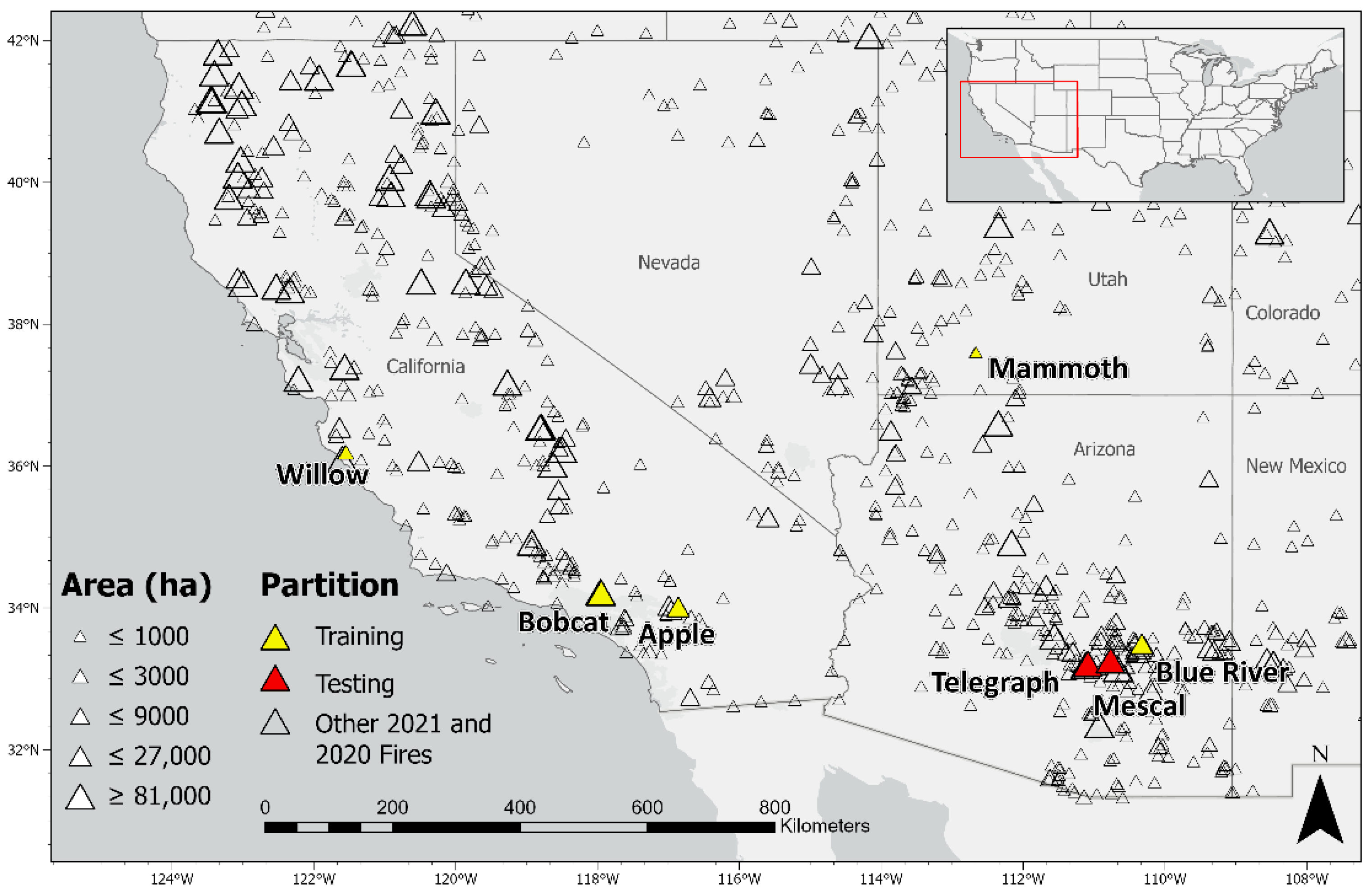
We focused on seven fires in the southwestern U.S. that occurred during the 2020 and 2021 fire seasons (Figure 1; Table 1). These same fires were analyzed as part of active wildfire mapping research [19]. The study sites, located in California, Arizona, and Utah, are characterized by hot and dry conditions with five of the sites dominated by scrub/shrub and the other two by conifer cover types.
This study relied on data from the European Space Agency’s Sentinel-2 multispectral sensor constellation. Sentinel-2 measures reflected energy in optical wavelengths from blue to short-wave infrared at 10-m to 60-m GSD [20]. The short-wave infrared (SWIR) bands are especially informative for active fire mapping as the energy in this wavelength can penetrate through moderate smoke; however, cloud cover may obscure all or portions of a fire. The Sentinel-2 constellation provides a 5-day revisit time at mid-latitudes, making it practical to utilize pre-application/post-application image differencing. Image differencing lowers the signal from unchanged surfaces while the signal from the features of interest (i.e., burn scar, retardant, etc.) is elevated. For long-duration fires, there is an opportunity for several image collections during the event.
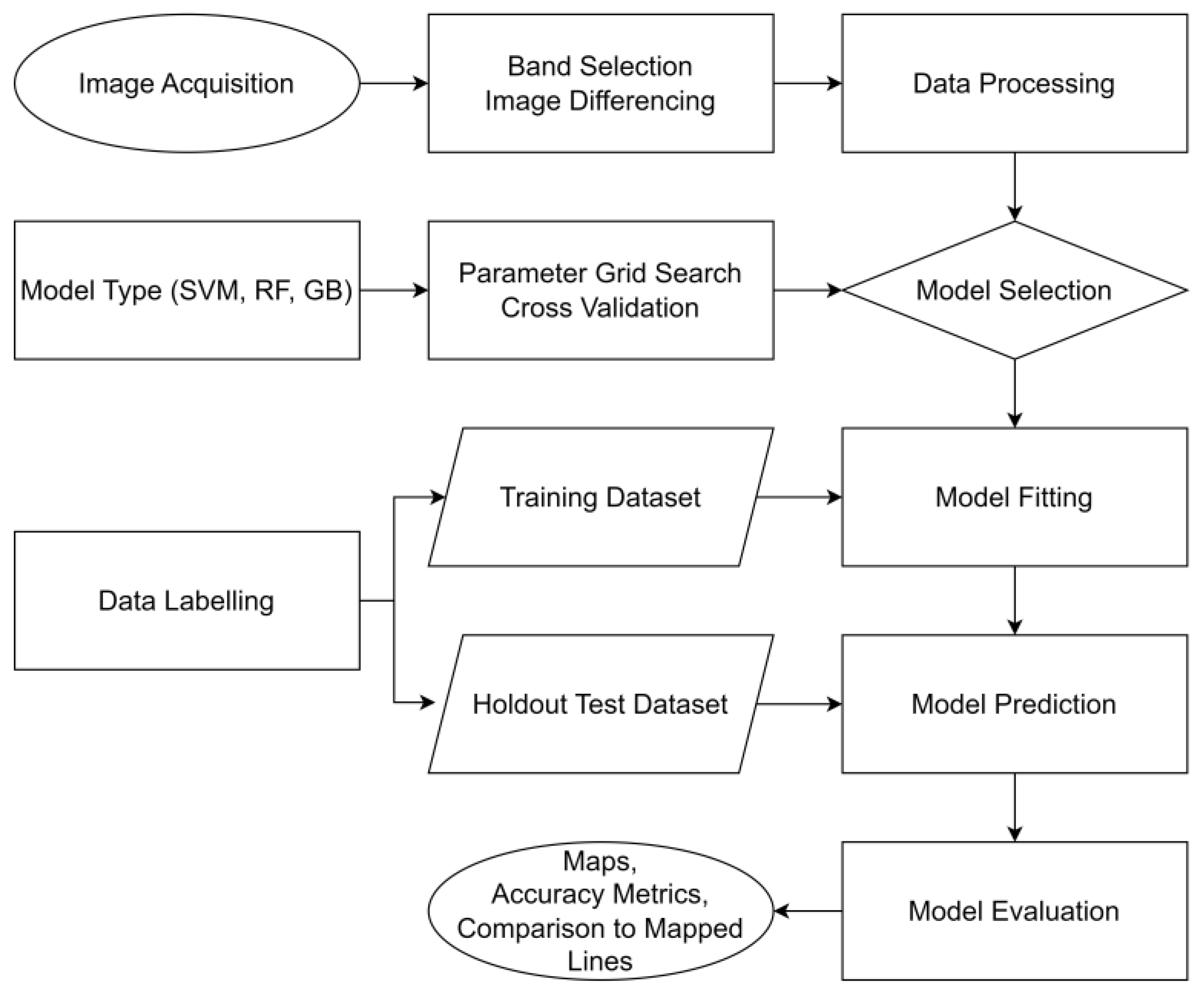
We used a supervised classification approach to discriminate the fire retardant from other image features. Three commonly-used machine learning classification models were trained for this application: random forest (RF), gradient boosting (GB), and support vector machine (SVM). The workflow implemented for these models is presented in Figure 2. These methods were selected because they are relatively mature in remote sensing [21] and have shown effectiveness for multispectral classification of land cover, fire, and other disturbance processes [22]. The random forest approach is commonly found to perform the best in terms of accuracy and processing efficiency [23,24], and is one of the most commonly applied methods in the domain of wildfire applications [17]. Additionally, these three models provide a baseline for testing against other machine-learning model architectures in the future.
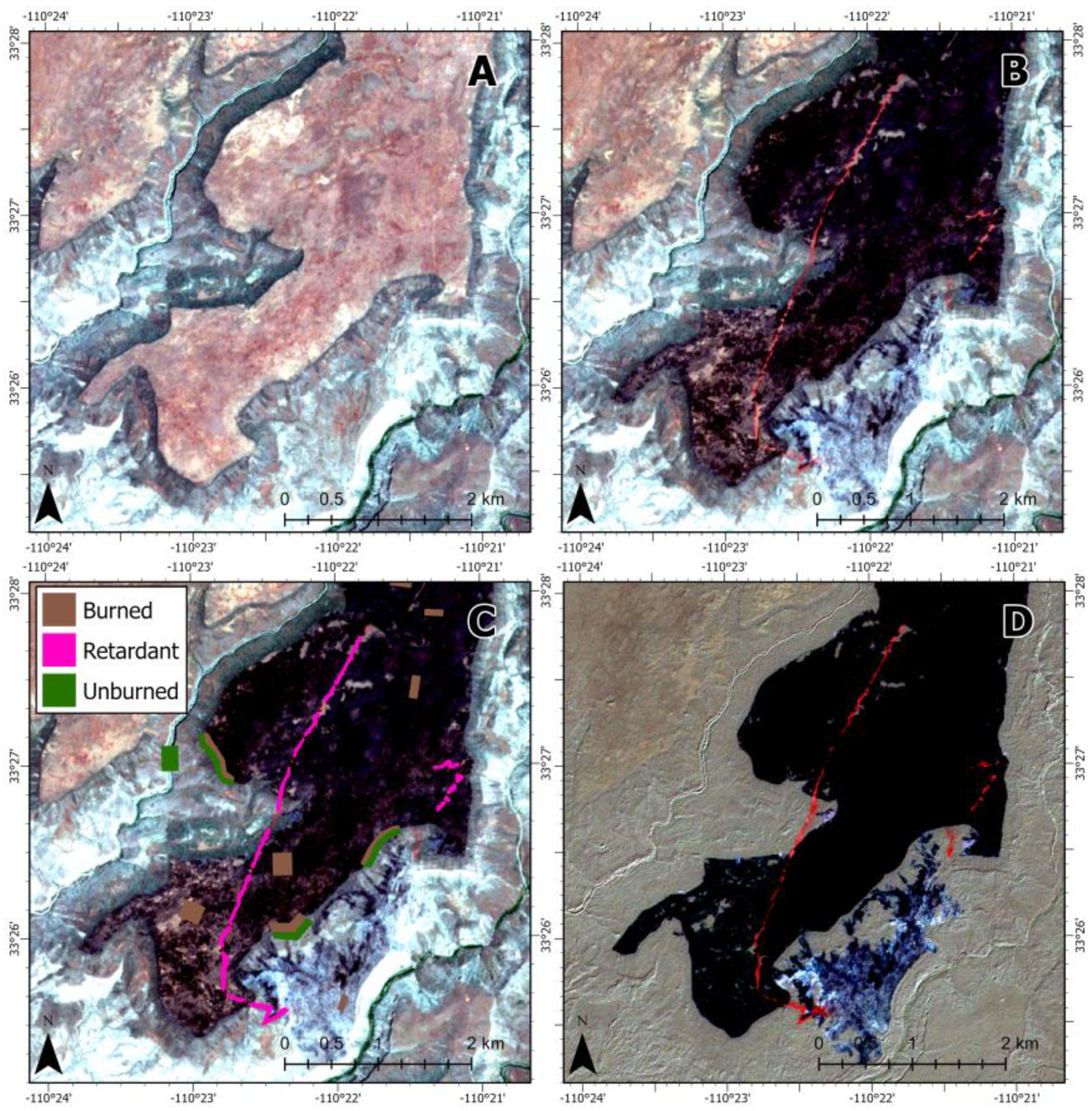
We trained and tested both single-class and multiclass classification approaches separately for post-application imagery (Figure 3B) and pre- and post-application difference images (Figure 3A,B,D). We collected training samples via visual interpretation of the imagery (Figure 3C). Training labels for the single-class model included presence/absence of fire retardant. The multiclass model included training labels for the following seven classes: retardant, burned, unburned, post-application cloud, pre-application cloud, post-application cloud shadow, and pre-application cloud shadow. For model selection, we employed a leave-one-group-out (LOGO) spatial cross-validation and a parameter grid search where each fire event was considered as a group in the spatial cross-validation. This emulates a real-world scenario wherein a model trained on past events is used to predict a current event (i.e., the left-out group). The parameter grid search tested all combinations of selected parameters to determine those that achieved the highest accuracy for the model. The model was then fit on data from all training sites and tested on a holdout test set. We produced the models in Python with the scikit-learn library (see Supplementary Material, Script S1: Model Training and Testing) as a per-pixel classification.
We assessed model performance using several common metrics including training and testing accuracy, precision, recall, and F1 score. Accuracy () represents the ratio of correctly predicted pixels to the total labeled pixels (Equation (1)).
where:
= number of true positive pixels
= number of false positive pixels
= number of false negative (missed) pixels
= number of true negative pixels
The precision () is the ratio of correctly predicted occurrences of a phenomenon (i.e., the presence of retardant in the pixel) to the total number of retardant pixels (Equation (2)).
The recall () is the ratio of correctly predicted retardant pixels to all the labeled retardant pixels (Equation (3)).
The F1 score is the weighted average of the precision and recall values, considering both types of errors, false positives and false negatives (Equation (4)).
3. Results
To assess model performance, we calculated the overall accuracy (Equation (1)), precision (Equation (2)), recall (Equation (3)), and F1 score (Equation (4)) using the test datasets for the Telegraph and Mescal fires in Arizona (Table 2). We report the overall accuracy for the best model in the parameter grid search fit to the training data (Table 3). To illustrate the error distribution between classes in the best model, a multiclass confusion matrix is included in the Supplementary Material (Table S1).
All three models had comparable accuracy metrics; however, the multiclass classification and difference imagery models consistently had the highest accuracies. Between SVM, RF, and GB, the GB model had the highest F1 score for fire retardant (0.76), though RF had a similar performance (0.74). Figure 4 presents the GB model predictions on the held-out test dataset. For comparison, the aerial GPS surveys for these fires are provided (dashed lines) in Figure 4A,C,E. The model predictions shown in Figure 4B (Telegraph, AZ) covers all field-surveyed retardant. Figure 4D (Telegraph, AZ) reveals retardant that was applied but was not captured in the aerial survey. In Figure 4E (Mescal, AZ), the model captures the most apparent retardant but also includes some inconsistent patches along droplines and some isolated false positives.
4. Discussion
The pre- and post-application difference images provide the best discrimination of retardant coverage. Overall accuracies and F1 scores from these images exceed those from post-application images for each model and class matrix. A better measure of success in mapping retardant locations might be gleaned by looking at the recall metric, which measures the ability to correctly classify targets that occupy a minor fraction of the overall image (e.g., retardant on the landscape). The recall values from the difference images are 2–10× higher than those from post-application images, indicating that the post-application-only image classifications are missing many pixels of retardant that could be mapped effectively via the difference images. The study area, which includes sites with iron oxide-rich surficial geology and soils, may represent increased confusion in the post-application-only images due to the iron oxide additive found in the fire retardant. After retardant application, the difference images show a stronger presence of iron oxide at drop sites, and a difference near zero in the background.
While most fires occur during warm and dry seasons, cloud cover is still an issue. At the time of model development, Sentinel-2 Level 1C data did not include a cloud mask, and cloud shadows were troublesome for the model. The application of modern cloud and cloud shadow masking algorithms would provide the ability to remove these areas from the model and reduce the potential for confusion between classes. This study did not develop or apply a cloud/cloud shadow mask; rather, we created labels for pre-application and post-application instances of clouds and shadows. An effective cloud and cloud shadow mask should improve the technique’s overall accuracy. Additionally, a map of the retardant area would be more informative if the classes (or masked areas) were represented as “unknown” or “cloud obscured”.
The model accuracy differences for the most effective combination of classes and images were relatively small, as measured by the F1 score (SVM, RF, and GB scored 0.70, 0.74, and 0.76, respectively). Considering the small differences between the model scores, additional criteria might be considered when deciding which classification to use. The main difference between RF and GB lies in how the decision trees are built. Unlike RF, the decision trees in GB are built additively (i.e., each decision tree is built one after another); thus, it is slower to train and suffers from potential overfitting. The SVM model is computationally expensive in relation to the RF and GB and, therefore, may be considered less attractive for the task of classifying many pixels over a large area. In light of these issues, the RF model may be preferred.
The results of this analysis are promising, though the classification models we tested generally underpredict the presence of retardant. This is evidenced by the precision and recall numbers for the best-performing model (0.999 and 0.615, respectively). The precision value, or producer accuracy, illustrates that the retardant identified by the model is very likely to be present (i.e., 99% likely). The recall value, or user accuracy, implies that the total number of retardant pixels mapped may be underpredicted by 38.5%. The underprediction is likely the result of a lower signal from the edges of the retardant line, where the retardant is diffuse enough to be confused with the background.
We developed and tested an approach to detect fire retardant using Sentinel-2 Level 1C data from the European Space Agency. The methods developed here could also be applied to other high-resolution multispectral sensors, including Landsat 8, Landsat 9, and WorldView-3, which have similar spectral bands (including SWIR bands). If this approach were to be employed operationally, an increased number of sensors would improve observation cadence and utility in wildfire management. Most spaceborne optical sensors lack a SWIR band which, for this application, ranked highest in band importance; thus, sensors without SWIR may struggle to achieve the same accuracy presented here (see Supplementary Material for test results on band importance Table S2). However, the combination of higher spatial resolution commercial sensors and more complex machine learning models may offer a solution that makes up for the lack of a SWIR band. For example, deep learning architectures like multilayer perceptron (MLP), long short-term memory (LSTM), and 2D or 3D convolutional neural networks (CNNs) may provide comparable results with less ideal spectral data. CNN-based models use pixel convolutions to implicitly learn textures, shapes, and edges of objects in imagery [24] which could be valuable in discriminating the retardant.
Five of the seven study sites over the southwest US are characterized by scrub/shrub cover types. Though retardant drops are likely more effective in these non-forested fuel types [25], models should be tested and updated over a wider geographic region, including more variable cover types.
Future studies would benefit from ground truth that includes detail on the aerial application rate of retardant (i.e., gallons per drop length) and concentration rate of ground-applied fire retardant (i.e., mass per unit area). With these types of data, new models could be developed to quantify the application rate of retardant, rather than just the drop footprint.
5. Conclusions
The aim of this short technical communication is to introduce the concept of using spaceborne optical data to rapidly and automatically detect and map wildfire retardant drop locations. We trained and tested a single-class and multiclass classifier using three commonly used machine learning models on two image sets (post-application only and pre-event and post-application difference imagery) across seven study sites. This study provides a baseline fire retardant detection capability to build from, including testing of different machine learning architectures, training/testing in more diverse cover types, and integrating additional sensors. All three models performed comparatively well, with the GB classification model achieving the highest accuracy and F1 score. The image differencing approach was highly effective in increasing the accuracy of the retardant classification. We show that the automated detection of recently dropped retardant is viable and improves the mapping product from an approximate centerline to a polygon area. This concept has the potential to improve active wildfire management by providing fire managers with more timely information on drop location, extent, and effectiveness, in addition to increasing safety by minimizing the need for aerial survey crews in an already busy and complex airspace. Further, the post-fire documentation of retardant placement near ecologically sensitive areas, and the potential to validate the cost of retardant drop services, can help improve process transparency.
Supplementary Materials
The supporting information can be downloaded at https://www.mdpi.com/article/10.3390/rs15020342/s1, Table S1: Confusion Matrix; Table S2: Model Feature Importances; Table S3: Scene ID; Script S1: Model Training and Testing; Script S2: Model Prediction.
Author Contributions
Discovery, J.D.T.; conceptualization J.D.T. and A.M.C.; methodology J.D.T. and T.M.S.; software T.M.S.; results analysis T.M.S. and J.T; writing-original draft preparation, J.D.T.; writing-review and editing, J.D.T., T.M.S. and A.M.C.; project administration, A.M.C.; funding acquisition, A.M.C. All authors have read and agreed to the published version of the manuscript.
Funding
This work was supported by the United States Department of Defense Joint Artificial Intelligence Center and the United States Department of Energy’s Office of Artificial Intelligence Technology Office (DOE-AITO) (contract no. HC1085017988), and the United States Department of Energy’s Office of Cybersecurity, Energy Security, and Emergency Response (DOE-CESER) (agreement no. M620000064).
Data Availability Statement
Data is contained within the Supplementary Materials.
Acknowledgments
The authors would like to thank Lee Miller for his careful review and suggestions, the anonymous reviewers for their time and insights, and Rick Stratton at the United States Forest Service for validating the interest in the application.
Conflicts of Interest
The authors declare no conflict of interest. The funders had no role in the design of the study; in the collection, analyses, or interpretation of data; in the writing of the manuscript; or in the decision to publish the results.
References
- Stonesifer, C.S.; Calkin, D.E.; Thompson, M.P.; Belval, E.J. Is This Flight Necessary? The Aviation Use Summary (AUS): A Framework for Strategic, Risk-Informed Aviation Decision Support. Forests 2021, 12, 1078. [Google Scholar] [CrossRef]
- Calkin, D.E.; Stonesifer, C.S.; Thompson, M.P.; McHugh, C.W. Large airtanker use and outcomes in suppressing wildland fires in the United States. Int. J. Wildland Fire 2014, 23, 259–271. [Google Scholar] [CrossRef]
- Plucinski, M.P.; Pastor, E. Criteria and methodology for evaluating aerial wildfire suppression. Int. J. Wildland Fire 2013, 22, 1144–1154. [Google Scholar] [CrossRef]
- Giménez, A.; Pastor, E.; Zárate, L.G.; Planas, E.; Arnaldos, J. Long-term forest fire retardants: A review of quality, effectiveness, application and environmental considerations. Int. J. Wildland Fire 2004, 13, 1–15. [Google Scholar] [CrossRef]
- USDA. Nationwide Aerial Application of Fire Retardant on National Forest System Lands; USFS, Ed.; USDA: Washington, DC, USA, 2020.
- USDA. Aerial Firefighting Use and Effectiveness (AFUE) Report; USFS, Ed.; USDA: Washington, DC, USA, 2020.
- Pérez, Y.; Pastor, E.; Planas, E.; Plucinski, M.; Gould, J. Computing forest fires aerial suppression effectiveness by IR monitoring. Fire Saf. J. 2011, 46, 2–8. [Google Scholar] [CrossRef]
- Pastor, E.; Planas, E. Infrared imagery on wildfire research. Some examples of sound capabilities and applications. In Proceedings of the IEEE 2012 3rd International Conference on Image Processing Theory, Tools and Applications (IPTA), Istanbul, Turkey, 15–18 October 2012. [Google Scholar]
- Jazebi, S.; de Leon, F.; Nelson, A. Review of wildfire management techniques—Part I: Causes, prevention, detection, suppression, and data analytics. IEEE Trans. Power Deliv. 2019, 35, 430–439. [Google Scholar] [CrossRef]
- Szpakowski, D.M.; Jensen, J.L. A review of the applications of remote sensing in fire ecology. Remote Sens. 2019, 11, 2638. [Google Scholar] [CrossRef] [Green Version]
- Barmpoutis, P.; Papaioannou, P.; Dimitropoulos, K.; Grammalidis, N. A review on early forest fire detection systems using optical remote sensing. Sensors 2020, 20, 6442. [Google Scholar] [CrossRef] [PubMed]
- Ambrosia, V.; Zajkowski, T.; Quayle, B. Near-Real-Time Earth Observation Data Supporting Wildfire Management. In Proceedings of the 2013 AGU Fall Meeting, San Francisco, CA, USA, 9–13 December 2013. [Google Scholar]
- Allison, R.S.; Johnston, J.M.; Craig, G.; Jennings, S. Airborne optical and thermal remote sensing for wildfire detection and monitoring. Sensors 2016, 16, 1310. [Google Scholar] [CrossRef] [PubMed] [Green Version]
- Wu, Y.; Arapi, A.; Huang, J.; Gross, B.; Moshary, F. Intra-continental wildfire smoke transport and impact on local air quality observed by ground-based and satellite remote sensing in New York City. Atmos. Environ. 2018, 187, 266–281. [Google Scholar] [CrossRef]
- Serra-Burriel, F.; Delicado, P.; Prata, A.T.; Cucchietti, F.M. Estimating heterogeneous wildfire effects using synthetic controls and satellite remote sensing. Remote Sens. Environ. 2021, 265, 112649. [Google Scholar] [CrossRef]
- Chuvieco, E.; Aguado, I.; Salas, J.; García, M.; Yebra, M.; Oliva, P. Satellite remote sensing contributions to wildland fire science and management. Curr. For. Rep. 2020, 6, 81–96. [Google Scholar] [CrossRef]
- Jain, P.; Coogan, S.C.P.; Subramanian, S.G.; Crowley, M.; Taylor, S.W.; Flannigan, M.D. A review of machine learning applications in wildfire science and management. Environ. Rev. 2020, 28, 478–505. [Google Scholar] [CrossRef]
- Lentile, L.B.; Holden, Z.A.; Smith, A.M.S.; Falkowski, M.J.; Hudak, A.T.; Morgan, P.; Lewis, S.A.; Gessler, P.E.; Benson, N.C. Remote sensing techniques to assess active fire characteristics and post-fire effects. Int. J. Wildland Fire 2006, 15, 319–345. [Google Scholar] [CrossRef]
- Coleman, A. Rapid Analytics for Disaster Response—Wildfire (RADR-Fire). In Proceedings of the Tactical Fire Remote Sensing Advisory Committee Meeting, Online, 11–13 May 2021. [Google Scholar]
- Drusch, M.; Del Bello, U.; Carlier, S.; Colin, O.; Fernandez, V.; Gascon, F.; Hoersch, B.; Isola, C.; Laberinti, P.; Martimort, P.; et al. Sentinel-2: ESA’s optical high-resolution mission for GMES operational services. Remote Sens. Environ. 2012, 120, 25–36. [Google Scholar] [CrossRef]
- Maxwell, A.E.; Warner, T.A.; Fang, F. Implementation of machine-learning classification in remote sensing: An applied review. Int. J. Remote Sens. 2018, 39, 2784–2817. [Google Scholar] [CrossRef] [Green Version]
- Sheykhmousa, M.; Mahdianpari, M.; Ghanbari, H.; Mohammadimanesh, F.; Ghamisi, P.; Homayouni, S. Support vector machine versus random forest for remote sensing image classification: A meta-analysis and systematic review. IEEE J. Sel. Top. Appl. Earth Obs. Remote Sens. 2020, 13, 6308–6325. [Google Scholar] [CrossRef]
- Hultquist, C.; Chen, G.; Zhao, K. A comparison of Gaussian process regression, random forests and support vector regression for burn severity assessment in diseased forests. Remote Sens. Lett. 2014, 5, 723–732. [Google Scholar] [CrossRef]
- Saltiel, T.M.; Dennison, P.E.; Campbell, M.J.; Thompson, T.R.; Hambrecht, K.R. Tradeoffs between UAS spatial resolution and accuracy for deep learning semantic segmentation applied to wetland vegetation species mapping. Remote Sens. 2022, 14, 2703. [Google Scholar] [CrossRef]
- Lawrence, R.L.; Moran, C.J. The AmericaView classification methods accuracy comparison project: A rigorous approach for model selection. Remote Sens. Environ. 2015, 170, 115–120. [Google Scholar] [CrossRef]
Figure 1.
Study sites for the machine learning model (filled symbols) with all fires ≥ 40 ha in size from 2020 and 2021 (open symbols). The symbols are scaled to the final burn area.
Figure 1.
Study sites for the machine learning model (filled symbols) with all fires ≥ 40 ha in size from 2020 and 2021 (open symbols). The symbols are scaled to the final burn area.

Figure 2.
The model workflow implemented in this study (SVM = support vector machine; RF = random forest; GB = gradient boosting).
Figure 2.
The model workflow implemented in this study (SVM = support vector machine; RF = random forest; GB = gradient boosting).

Figure 3.
Sentinel-2 true-color imagery from the Blue River (Arizona, 2020) fire: (A) pre-application; (B) post-application; (C) post-application with reference labels; (D) difference image post-application minus pre-application.
Figure 3.
Sentinel-2 true-color imagery from the Blue River (Arizona, 2020) fire: (A) pre-application; (B) post-application; (C) post-application with reference labels; (D) difference image post-application minus pre-application.

Figure 4.
Gradient boosting model predictions on the held-out test dataset. Dashed lines show aerial GPS surveys (left panel images). (A) Telegraph, AZ post-application true-color imagery; (B) model prediction for (A); (C) Telegraph, AZ post-application true-color imagery; (D) model prediction for (C); (E) Mescal, AZ post-application true-color imagery; (F) model prediction for (E).


Table 1.
Fire incident and imagery details. Scene ID’s can be found in Supplemental Material, Table S3: Scene ID.
Table 1.
Fire incident and imagery details. Scene ID’s can be found in Supplemental Material, Table S3: Scene ID.
| Incident Name | Year | Fire Start | Fire End | Pre-Image | Post-Image | Location | Size (ha) |
|---|---|---|---|---|---|---|---|
| Apple | 2020 | Jul 31 | Nov 16 | Jul 27 | Aug 08 | Cherry Valley, CA | 13,526 |
| Blue River | 2020 | Jun 05 | Jun 18 | May 29 | Jun 08 | 15 mi NE of San Carlos, AZ | 11,352 |
| Bobcat | 2020 | Sep 06 | Oct 19 | Aug 01 | Sep 20 | Azusa, CA | 46,861 |
| Mammoth | 2021 | Jun 05 | Jun 20 | Jun 01 | Jun 11 | Mammoth Creek, UT | 287 |
| Mescal | 2021 | Jun 01 | Jun 18 | Jun 03 | Jun 13 | Globe, AZ | 29,239 |
| Willow | 2021 | Jun 17 | Jul 11 | Jun 13 | Jun 23 | Arroyo Seco, CA | 1164 |
| Telegraph | 2021 | Jun 04 | Jul 08 | Jun 03 | Jun 13 | Superior, AZ | 73,150 |
Table 2.
Model testing results with different data scenarios: binary, multiclass, post-application, and pre- and post-application difference images (* denotes the best model).
Table 2.
Model testing results with different data scenarios: binary, multiclass, post-application, and pre- and post-application difference images (* denotes the best model).
| Model | Classification | Imagery | Train Overall Accuracy | Test Overall Accuracy | Test Retardant Precision | Test Retardant Recall | Test Retardant F1 Score |
|---|---|---|---|---|---|---|---|
| RF | Single-class | Difference | 0.928 | 0.949 | 0.998 | 0.544 | 0.705 |
| RF | Single-class | Post-application | 0.935 | 0.916 | 0.996 | 0.253 | 0.404 |
| RF | Multiclass | Difference | 0.809 | 0.873 | 0.997 | 0.589 | 0.74 |
| RF | Multiclass | Post-application | 0.815 | 0.822 | 0.997 | 0.245 | 0.393 |
| SVM | Single-class | Difference | 0.933 | 0.938 | 0.978 | 0.46 | 0.626 |
| SVM | Single-class | Post-application | 0.945 | 0.898 | 0.993 | 0.091 | 0.167 |
| SVM | Multiclass | Difference | 0.812 | 0.912 | 0.99 | 0.549 | 0.706 |
| SVM | Multiclass | Post-application | 0.837 | 0.813 | 0.992 | 0.091 | 0.167 |
| GB | Single-class | Difference | 0.936 | 0.947 | 0.999 | 0.531 | 0.693 |
| GB | Single-class | Post-application | 0.942 | 0.893 | 0.998 | 0.051 | 0.097 |
| GB | Multiclass | Difference | 0.814 | 0.881 | 0.999 | 0.615 | * 0.761 |
| GB | Multiclass | Post-application | 0.825 | 0.8 | 0.998 | 0.052 | 0.1 |
Table 3.
Individual class accuracy metrics of the best model (GB, Multiclass, Difference) on the test data set.
Table 3.
Individual class accuracy metrics of the best model (GB, Multiclass, Difference) on the test data set.
| Class | Precision | Recall | F1 Score |
|---|---|---|---|
| Retardant | 0.999 | 0.615 | 0.761 |
| Burned | 0.803 | 0.999 | 0.890 |
| Unburned | 0.920 | 0.997 | 0.957 |
| Cloud post-application | 0.883 | 0.875 | 0.879 |
| Cloud pre-application | 0.714 | 0.583 | 0.642 |
| Shadow post-application | 0.605 | 0.330 | 0.427 |
| Shadow pre-application | 0.960 | 0.855 | 0.904 |
Disclaimer/Publisher’s Note: The statements, opinions and data contained in all publications are solely those of the individual author(s) and contributor(s) and not of MDPI and/or the editor(s). MDPI and/or the editor(s) disclaim responsibility for any injury to people or property resulting from any ideas, methods, instructions or products referred to in the content. |
© 2023 by the authors. Licensee MDPI, Basel, Switzerland. This article is an open access article distributed under the terms and conditions of the Creative Commons Attribution (CC BY) license (https://creativecommons.org/licenses/by/4.0/).
Share and Cite
MDPI and ACS Style
Tagestad, J.D.; Saltiel, T.M.; Coleman, A.M. Rapid Spaceborne Mapping of Wildfire Retardant Drops for Active Wildfire Management. Remote Sens. 2023, 15, 342. https://doi.org/10.3390/rs15020342
AMA Style
Tagestad JD, Saltiel TM, Coleman AM. Rapid Spaceborne Mapping of Wildfire Retardant Drops for Active Wildfire Management. Remote Sensing. 2023; 15(2):342. https://doi.org/10.3390/rs15020342
Chicago/Turabian StyleTagestad, Jerry D., Troy M. Saltiel, and André M. Coleman. 2023. "Rapid Spaceborne Mapping of Wildfire Retardant Drops for Active Wildfire Management" Remote Sensing 15, no. 2: 342. https://doi.org/10.3390/rs15020342
Note that from the first issue of 2016, this journal uses article numbers instead of page numbers. See further details here.