

Compression of GNSS Data with the Aim of Speeding up Communication to Autonomous Vehicles

1
Computer Science Department, Holon Institute of Technology, Holon 5810201, Israel
2
Computer Science Department, Bar-Ilan University, Ramat-Gan 5290002, Israel
*
Author to whom correspondence should be addressed.
Remote Sens. 2023, 15(8), 2165; https://doi.org/10.3390/rs15082165
Submission received: 6 March 2023
/
Revised: 1 April 2023
/
Accepted: 13 April 2023
/
Published: 19 April 2023
(This article belongs to the Special Issue Advanced Technologies for Position and Navigation under GNSS Signal Challenging or Denied Environments II)
Abstract
:Autonomous vehicles contain many sensors, enabling them to drive by themselves. Autonomous vehicles need to communicate with other vehicles (V2V) wirelessly and with infrastructures (V2I) like satellites with diverse connections as well, to implement safety, reliability, and efficiency. Information transfer from remote communication appliances is a critical task and should be accomplished quickly, in real time and with maximum reliability. A message that arrives late, arrives with errors, or does not arrive at all can create an unsafe situation. This study aims at employing data compression to efficiently transmit GNSS information to an autonomous vehicle or other infrastructure such as a satellite with maximum accuracy and efficiency. We developed a method for compressing NMEA data. Furthermore, our results were better than other ones in current studies, while supporting error tolerance and data omission.
1. Introduction
Autonomous vehicles [1,2] are able to control a full car system in collaboration with human interaction. Sometimes, the vehicle’s control and computer system can also take full control when the driver cannot handle them, as in falling asleep behind the steering wheel, experiencing an emergency medical situation, or undergoing a vehicle emergency due to a flat tire or a mechanical problem. One of the challenges today is gaining public trust in the concept of autonomous driving [3].
Today, technology giants and automakers have been working toward full automation with the goal of selling cars that can drive safely and efficiently with an emphasis on reducing GNSS errors [4]. In our former paper, we explained the correlation between compression and errors [5].
Ideally, essential information passes in a fraction of a second and without delays and losses. Unfortunately, navigation software is often slow in delivering initial results, or, when there are no satellite signals, the navigation software works well because it receives wrong data. The compression and decompression methods presented in this investigation endeavor to improve this situation.
We review in this paper some relevant aspects of the suggested system—autonomous vehicles, Data Compression, GNSS devices and the NMEA Standard [6]. We deal with several compression methods, some of them known; however, we made an effort to produce a new (hybrid) method that is based on known methods and algorithms.
During our research, we noticed that adjacent frames of GNSS data are frequently very similar; accordingly, we looked for a compression method that efficiently works with differences to prepare the data for an entropy encoder like Huffman coding. We analyzed several compression methods, eliminating ones like JPEG2000 [7] because, not making use of the comparison of frames, they were unsuitable for our method as a preprocessing step.
The aim of this work is not to correct errors but to suggest a time-saving method to transmit information with no less reliability than raw information transmission. If the original information is invalid, our algorithm will filter out the errors before the compression process begins, as can be seen in Figure A3 in Appendix A.
Many kinds of data like video, audio, images, and many other information files are usually compressed. Therefore, it is very important to have good and fast compression and decompression methods for many applications in autonomous vehicles.
The method presented below is very similar to the well-known H.264. It is a relatively simple standard that plays an important role in many consumer electronics applications, including VCDs, DVDs, video phones, portable media players, video conferencing, video recording, e-learning, etc. It is mainly employed when there is a need to find solutions of relatively high quality, low transmission rate and good compression ratios [8,9]. H.264 takes advantage of the frequent similarity of adjacent frames. GNSS systems usually produce information that also has this attribute of similarity between adjacent blocks; thus, we have adapted the concept of H.264.
During this research, an algorithm that is a cornerstone and foundation in computer science, Huffman coding, was used as part of the compression process. Using this algorithm, we have achieved particularly high durability and survivability compared to other existing methods. In this study we investigate and show different methods for compressing GNSS data in vehicles to a good level of about 12% with the critical attribute of error correction.
The rest of this paper is organized as follows: Section 2 gives a background of autonomous vehicles, data compression, GNSS, and the NMEA standard. Section 3 reviews literature and related works on GNSS data compression. Section 4 explains how and why we employ H.264-like compression. Section 6 describes the testbed for our experiments. Section 7 presents the results while Section 8 concludes and discusses the implications of this research and future investigations.
2. Background
2.1. Autonomous Vehicles
By using autonomous vehicles, we endeavor to reduce human errors (currently responsible for more than 90% of accidents), but there are also machine errors [10].
One of the causes of safety failure is a delay in information transfer between V2V autonomous vehicles or between autonomous vehicles and infrastructures such as the GNSS (V2I). Unlike traditional vehicles, autonomous vehicles transmit a considerable amount of information over a network. Therefore, it is essential to take care of data compression to reduce the amount of information that needs to be sent and, as a result, increase the speed of information transmission.
2.2. Data Compression
Data compression is usually used to save storage and to reduce data transmission, thereby speeding up transmission of data from one endpoint to another. We can compress not only text but also images, audio, and video files. Several techniques of data compression, such as Huffman Code, Shannon Fano Code, and Lempel Ziv are designed to ensure that the size of the compressed file is smaller than the original [13,14].
As in many contemporary applications, we will make use of the Huffman Codes [15] because they can easily recover from errors and faults.
The Huffman Codes were invented in 1952 by a student who studied with Prof. Fano from MIT. At the time, the Shannon-Fano Codes were the best available method for data compression. While Huffman was thinking about doing research, however, he came up with an algorithm called “Symbol Coding Method”, “Prefix Coding” or “Huffman Coding”. This compression technique offers encoding symbols such as text characters without data loss [16].
The Huffman Codes are an algorithm that belongs to a group called prefix codes. This algorithm provides good data compression and stores the items in a minimum number of bits when their frequency is high—according to the probabilities at which each item appears. This method is based on assigning a variable-length code to each item according to its frequency, so that a frequent item will be represented by a small number of bits whereas an infrequent item will be represented by a longer code.
Huffman’s coding has a legendary and important status in the field of computer science and engineering, for its simplicity and applicability make it an idyllic example in algorithm courses. Moreover, it is one of the most common techniques used for data compression [17].
2.3. Global Navigation Satellite System
The Global Navigation Satellite System (GNSS) makes use of satellites in space around the Earth. The idea began in the 1970s among the U.S. military as Americans sought a way to overcome the difficulties of previous navigation systems in use. GNSS began to be extensively used in the 1990s [18].
The principle of the GNSS is sending the location of the transmitter to the receiver in space (satellite) and next retrieving information from the receiver to the transmitter on Earth [19]. GNSS transmitters require access to open skies; otherwise, interference or loss of GNSS signals can occur. This type of communication experiences failures in areas where construction is very high or in areas of forests or mountains. GNSS tracking is applied in a variety of fields, including animals, car travel, hiking, and even sports [20,21,22].
The GNSS device is essential to autonomous vehicles in need of high availability and accuracy. A vehicle can plot a pre-known or pre-programmed route autonomously without any human control [23]. Therefore, it is very important that an autonomous vehicle is able to receive and send its location promptly to the mobile network and/or satellite communication. A major advantage of using GNSS is that the data do not depend on previously received information and therefore localization errors do not accumulate over time.
One of the GNSS’s essential attributes is its accuracy, which depends on the environment in which the GNSS transmitter is located and the number of satellites it reads at any given time, alongside the location of the transmitter and the environment in which it is located: for example, in an urban environment, underground parking, a forest, or an open space.
2.4. NMEA Standard
The NMEA (National Marine Electronics Association) standard, also known as Standard 0183, was introduced in 1983 as a standard for data communication between ships. The NMEA protocol uses ASCII codes, and the data transfer is slow at 4800 bytes per second. However, it is still widely used and is perfectly suited to situations where one end, such as a GNSS device, needs to be connected to another end, such as a satellite [24,25].
The default transmission rate of the NMEA GNSS standard is 4.8 kb/s. It uses 8 bits for the data of ASCII characters and 1 stop bit. More than a few years later, the NMEA2000 protocol, much more advanced than the previous one, was invented. The new protocol allows multiple units to transmit and receive data simultaneously; its cables are less sensitive to noise (with wired connections) and its information transfer is superior to that of NMEA0183.Furthermore, it allows data transfer rates up to 250 kb/s (about 50 times faster) [6].
The use of NMEA in ships is very significant and important because in the sea we do not have signs, and one of the options to navigate at sea in the modern world is through GNSS, in contrast with other transportation such as vehicles that can navigate the roads thanks to road signs and directions.
Most systems that provide real-time placement ensure that the data are in NMEA form. These data include, among others, PVT: Position, Velocity and Time [26]. Most often we will see standard NMEA sentences in any GNSS devices commercial production [27]. It is also possible to define unique, proprietary sentences for a particular purpose instead of existing ones. For example, a Garmin sentence would start with PGRM [28]. We discuss standard sentences below, and all the sentences have something in common.
Each NMEA sentence is represented by ASCII codes, starting with a $ sign and a prefix of “GP”, which defines GNSS receivers. Three letters mark this type of sentence [29].
For example, most popular types:
- GPGGA—fix information
- GPGSV—detailed satellite data
- GPRMC—recommended minimum data for GNSS.
- GPGSA—overall satellite data
Each NMEA sentence type can contain no more than 80 characters of plain text, with data items separated by commas. In each type of data, a checksum is included for the sentences. These begin with ‘*’ and two HEX digits representing the XOR action of all characters between the ‘$’ (not including) and up to ‘*’. A test amount is not required for all the sentences.
In autonomous vehicles and vehicles in general, NMEA sentences are used in the following formats: GPGGA, GPGSV, GPGSA, GPRMC [30].
3. GNSS Data Compression Review and Related Work
Today, the processors are very powerful and can process data and RAM rapidly. Nevertheless, a busy communication channel can be challenging. The busier the communication channel and the more information passes through it, the more information can be delayed. The transmission time is significantly greater than the processing time, which is negligible in the transmission time [31]. That is why previous investigations have assessed the amount of information transferred and not the processing times [32], A procedure we follow later in the results section.
Among several recent studies and articles about GNSS data compression, one that was recently carried out examined the compression of GNSS data in maritime usage by ships and vessels. To the best of our knowledge, there is no study of data compression originating from GNSS in combination with autonomous vehicles. This work reports on the ability to compress data at a very high efficiency’ obtaining a compression ratio of about 4% of the raw information [33]. However, naval vessels generally avoid turns due to their dimensions and usually perform only prearranged turns in very wide areas. Commonly, ships do not navigate many turns or U-turns, unlike vehicles, but rather go in straight lines [34]. Therefore, the changes in the GNSS information are typically small and yield a much better compression ratio.
A recently published paper explored and proposed GNSS data compression in IOT components and trajectory reconstruction. Unlike in our data, the authors of this paper consider several different trajectory typologies. They compress this data employing a combination of their suggested technique with a lossless compression method, trying as a lossless method the well-known methods—Huffman, LZ77 and LZW. Nonetheless, they came to a similar conclusion that combining the Huffman codes with another method indeed gives better results than just compressing the data using Huffman codes [35].
The subject of GNSS data compression has already previously been studied; however, the studies are from different directions with usually dissimilar approaches, unlike our research.
Some of the studies that have been done on the subject compress completely different information [36]. One proposed compression algorithm [37] requires accompanying hardware and other supporting equipment such as a server that performs data analysis, compression and transmission. Working with a server cannot be practical for our research because it works in a real time environment.
An algorithm more similar to our work is suggested in [38]. It analyzes NMEA data compression using some combinations with LZ77 and Huffman coding. The compression results in this paper are an output of about 30% of the original information. Furthermore, the writers have taken out some of the information so that all the records will have the same fields and the compression ratio will be enhanced. Even with these features, this paper achieved significantly inferior results because the differences method, such as H.264, which can substantially improve the performance, is not employed. In our research, we made use of H.264 and as a result were able to get much better results of about 13%.
The goal of compression is to efficiently reduce the amount of information transmitted by GNSS. Raw data transmitted by GNSS is very expensive, costing thousands of dollars per day and millions of dollars per year for only about 4000 vehicles that use it [39].
Today every vehicle (even non-autonomous) has built-in GNSS components [40], but the topic becomes very significant when we talk about GNSS in autonomous vehicles [41]. The amount of information that these vehicles transmit will be significantly bigger. One of the components constantly changed and transmitted across bandwidths is the location data of the vehicle.
This research presents a method for compressing GNSS data as a difference between location and time. An additional example can be found in [42], which shows that GNSS information contains many commas between the parameters. Commas are information repeated over and over again within the message [It undoubtedly takes up bandwidth and therefore needs to be more efficiently compressed (e.g., Huffman code).
In the algorithm discussed above, compressed information is transferred most of the time, but occasionally full information is transferred to avoid retaining errors over time.
4. Employing H.264-Like Compression
The main objectives of the H.264/AVC standardization efforts were improving the compression performance, providing “network-friendly” video representation, and compressing the information more efficiently than in previous standards, such as H.263 [43].
H.264/AVC represents advances in standard video encoding technology, improving encoding efficiency and flexibility for use in a wide range of networks and applications [43,44].
H.264 provides about 50%-bit rate savings for equal perceptual quality compared to the performance of previous standards, such as H.263 [45,46].
H.264 makes use of three frames (I- FRAMES, P-FRAMES and B- FRAMES) to improve error resilience, avoid failures in video streaming, and improve the efficiency of compression and the compressed stream [46,47,48].
Compression can be improved by further modifications, such as by using differences between time and location data and compressing the commas by using the Huffman Code. Moreover, vehicles often get stuck in traffic jams; the more vehicles, the bigger the traffic jams will be [49]. The average speed today in big cities can be even under 30 km/h, as in New York [50] or Tel Aviv (around 15 km/h).
Beyond the traffic jams, the vehicles idle at traffic lights or stop for various purposes. On all these occasions, the vehicle sends information about its location using the method described in [42] but with several changes.
In autonomous vehicles, several types of connections help vehicles to receive information from the environment (other AVs) and vice versa, as with vehicle-to-vehicle (V2V), vehicle-to-infrastructure (V2I), and vehicle-to-everything (V2X) [51].
H.264 takes advantage of the property that adjacent video frames are usually very similar. Therefore, the values of the adjacent blocks’ differences will be zero or close to zero. The more zeros we obtain, the better the Huffman coding efficiency. The information that GNSS generates also usually has this feature of similarity between adjacent blocks, so we adapted the idea of H.264 and achieved an effective and efficient preprocessing step.
We analyzed the GNSS data compression and decompression, which can affect the total time and resources used by the GNSS. The differences between the consequent NMEA sentences will be compressed in the way that H.264 handles consequent frames with small differences.
5. Methodology
This investigation was performed with several compression and optimization tools and methods, which we describe below, explaining their advantages and disadvantages. We furthermore explain why some of the methods achieved better results than others we tried but rejected. Our tool for compression and decompression was written by us in C#, along with another tool written by us, which aims at comparing results and checking them visually. Examples of output files from the C# tool are shown in Figure A1, Figure A2, Figure A3, Figure A4 and Figure A5. The visual tool is explained in more detail below in Section 7.
Accordingly, the algorithm for encoding a raw GNSS data file is (Algorithm 1):
| Algorithm 1: Compression GNSS data |
| Input: Raw GNSS data Output: compressed binary data
(V=invalid data).
|
Correspondingly, the algorithm for decoding data file is (Algorithm 2):
| Algorithm 2: Decompression GNSS data |
| Input: compressed binary data Output: Decompressed GNSS data
|
6. Experiments
Data was collected by traveling on many roads in several vehicles with the same receiver (smartphone). First, for data collection, the following NMEA LOGGER application was utilized during the trips [52].
This application allowed us to record NMEA data in raw form and transfer the data file to a computer for analysis and further analysis. The application is intended for use on smartphones using the Android operating system from Google Play. In our research, the NMEA LOGGER application version 2.3.35 was used on a Samsung S20 ULTRA device (Samsung Seoul, South Korea) running the Android operating system. Aiming at analyzing information and collecting data, we incorporated urban and intercity routes and interspersed long and short ranges.
This application can create a large log file with all the GNSS data and sub-protocols. We did not need some of the data for this study, so we filtered it for only the relevant data. Nowadays, a filtering method before analyzing results or performing actions is prevalent in many applications, as in [53].
Several short and long samples have been extracted and are shown in the tables that appear in the Results section. The shortest trip was about 50 km in 20 min, and the longest was about 4.5 h and 300 km, which included driving on a highway and standing in urban traffic jams.
In Figure A1 in Appendix A, we see many information lines not relevant to the content that we want to compress. For us it is a sort of noise that we have filtered out.
The content of the desirable protocols has been extracted. The extracted protocols are:
- GPGGA
- GPGSV
- GPGSA
- GPRMC
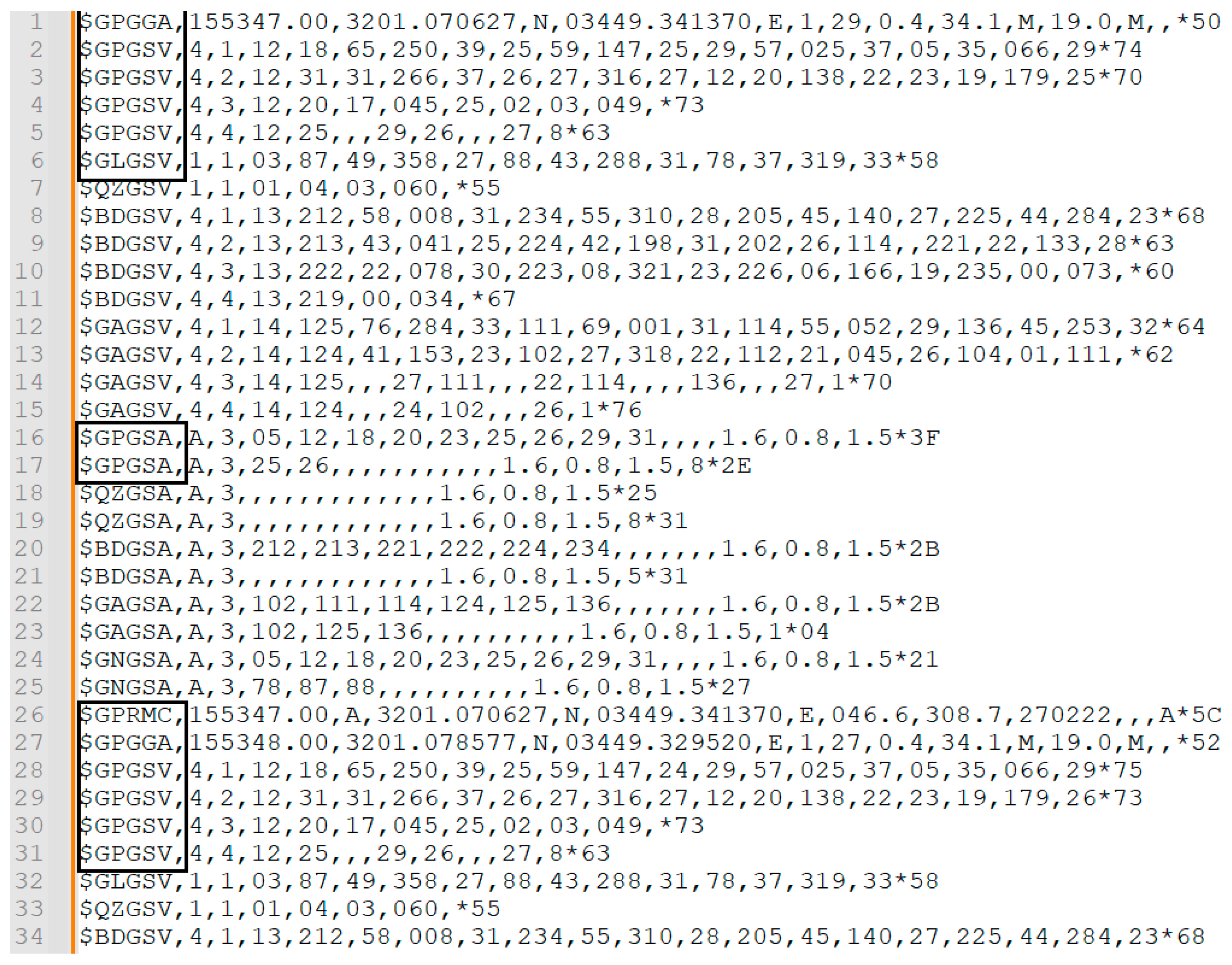
The contents of the desired protocols are extracted. After the filtering out of this noise, a new text file was built and through it, repeating patterns within each line of each protocol were examined. An example of a filtered file can be seen in Figure A2 in Appendix A, which includes only the four protocols mentioned above.
For example, one of the methods tried in the research was calculating differences between rows’ values in each block. This shows very good compression data, but it is very difficult to recover information, so we rejected this method.
Sometimes the vehicle sends or receives incorrect satellite information, which can happen for many reasons. For example, the vehicle enters an underground parking lot or tunnel, or a momentary malfunction occurs in the reception of GNSS satellites [54,55,56]. During the first step, it was decided to remove incorrect information.
In Figure A3 in Appendix A, we see noises in both the GPGSA and GPRMC protocols, which are incorrect data. These noises cause an omission of most of the information block that includes additional protocols, as seen, for example, in the GPRMC protocol when its third value is the V value, which means the information is incorrect. Also, incorrect information can be detected in the GPGSA protocol when the third parameter is 1 (Mode: 1 = Fix not available).
If there is incorrect information for any reason, the algorithm will delete most of the block with the incorrect information, as exemplified in Figure A3 in Appendix A.
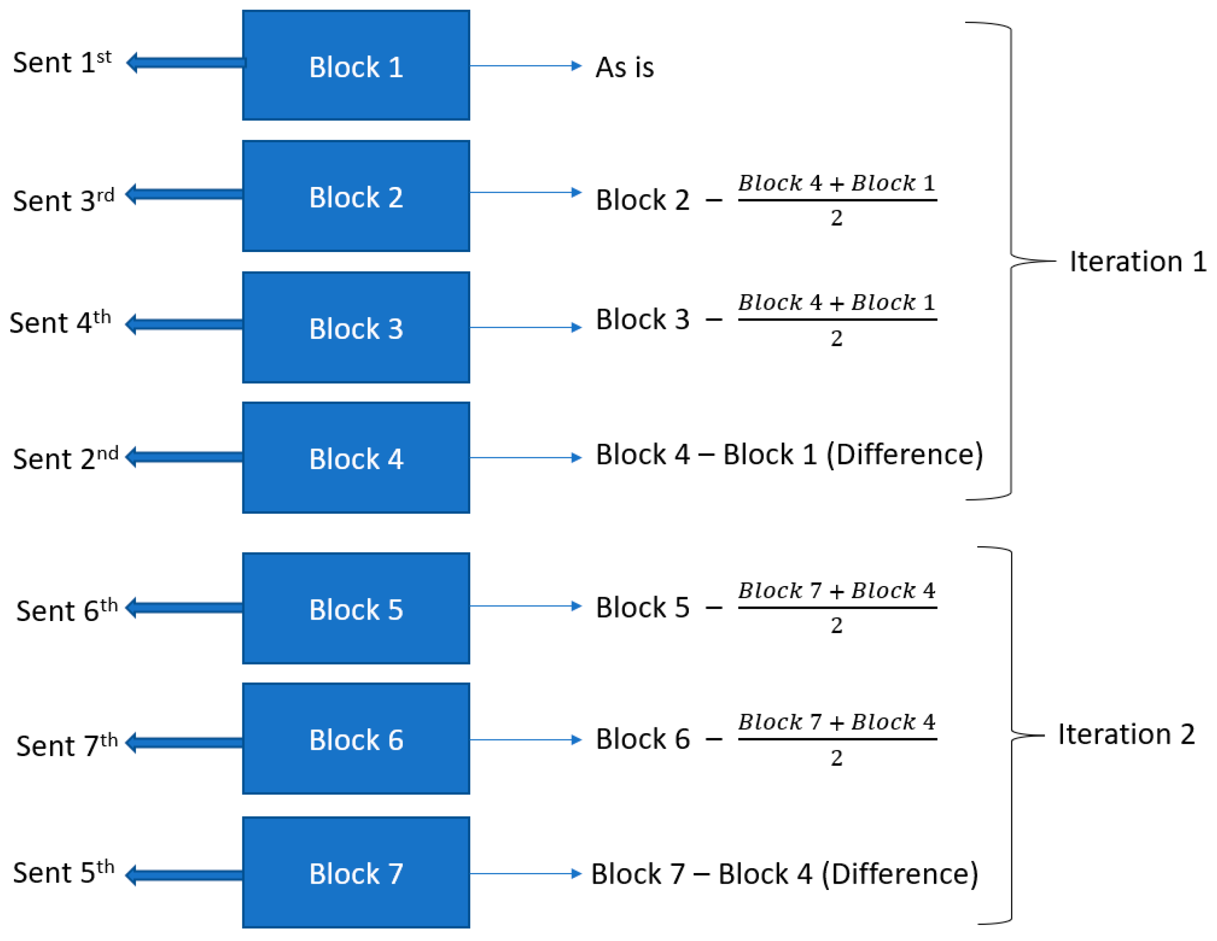
We suggest calculating differences between the rows with the same protocol like it is done in the H.264 method. For example, in each block there are k rows where:
- 5 ≤ k ≤ 13.
- GPGGA is a 1-line message.
- GPGSV is 1–9 lines of messages.
- GPGSA is 2-lines of messages.
- GPRMC is a 1-line message.
The example in Figure 1 demonstrates how it works:
One of the difficulties was with GPGSV. The challenge emerges when in certain blocks in the GPGSV protocol, we have a certain number of lines, and then after a few iterations, a block appears with the GPGSV protocol with a different number of lines (more lines or less).
Figure A4 in Appendix A shows a case with a different number of GPGSV lines. In iteration 4 (line 22–29), the GPGSV lines are not the same as the GPGSV lines of iteration 1 (line 1–7).
Since the H.264-like algorithm employs differences between iterations, it is important for us to have the same number of rows in each iteration to calculate a difference from another line or a difference from the average.
Monitoring and testing made it possible to see that the changes are made infrequently, so it was decided to split the file. That is, as soon as an iteration is received in which the number of lines in the GPGSV protocol differs from the previous number of lines, the file is closed, and a new file initialized with a number of lines in the latest GPGSV, and so on.
In the process of building a binary file, another problem was detected. When a computer writes a file, the size of the file will be rounded to a multiple of 8 bits because computers work with bytes. This caused a problem in the decoding stage as the decoding came out wrong due to the added bits at the end of the file.
As a result, it was decided to add another byte at the end of the binary file, in which it is indicated how many zeros that were added as padding must be removed from the previous byte.
An issue that should be handled occurs when there are lines from different iterations with different fields. Figure A5 in Appendix A shows such a case, where there is a value between the commas, and the algorithm needs to make a difference from a row from an upper block where there is no value between the commas (NULL) or vice versa. For such cases we used a special pattern, seen in Figure 2.
When a difference from the average must be calculated (as the B-frame in H.264), for example:
It would be helpful if the rows had matching fields or no values in the same fields (which are also matching), but sometimes, as shown above, in certain lines between commas contain a value compared to the average where there is no value between commas (or vice versa).
An example of this is:
- AVG EXAMPLE → (4 + 1)/2
- 1,2,3 = 1
- 1,2,3,4 = 4
- 1,2,3, EOL,4 = avg
- Or vice versa
- AVG EXAMPLE → (4 + 1)/2
- 1,2,3,4 = 1
- 1,2,3 = 4
- 1,2,3 = avg
It is possible to stop counting after and saving all the information after index 3 (4 + null) because iteration 1 (iterative) exists all the time and can be easily restored/decoded.
Similarly, when we calculate the average (AVG), for example, , there may be no values between commas in block 4 in a certain protocol compared to block 1 (or vice versa).
An example for such a case:
- AVG → (4 + 1)/2 (4 on the left, 1 on the right)
- 3,6,9, , = 1
- 1,2,3,4 = 4
- 2,4,6,#4 (complete to the left side of 4)
- Or vice versa:
- AVG → (4 + 1)/2 (4 on the left, 1 on the right)
- 3,6,9,5, = 1
- 1,2,3, , = 4
- 2,4,6, -#5 (minus means the number after # put on the right side of 1)
When a row in which we want to make a difference or a difference from the average, it is shorter (or longer) than a row from another block, respectively. That is, a certain row has more fields (or fewer) than a corresponding row.
An example of such a case:
- AVG → (4 + 1)/2
- 3,6,9 = 1
- 1,2,3,4,5,6,7 = 4
- 2,4,6, EOL,4,5,6,7 (once we see EOL we put all the info after EOL to left side of 4)
Another example is vice versa but a little bit different:
- AVG → (4 + 1)/2 (4 on the left, 1 on the right)
- 3,6,9,1,2,4 = 1
- 1,2,3,4 = 4
- 2,4,6
We stopped calculating after (9 + 3)/2 and we do not need to save all the information after index 4 (2 + null) because we have iteration 1 (it appears iteratively) all the time and it can be simply recovered/decoded.
After performing the actions mentioned above, we get a difference file, saving only around 28% in space. At this point, we achieve a file with many repeating zeroes, which allows us to use Huffman coding more efficiently and thus attain a better compression ratio later.
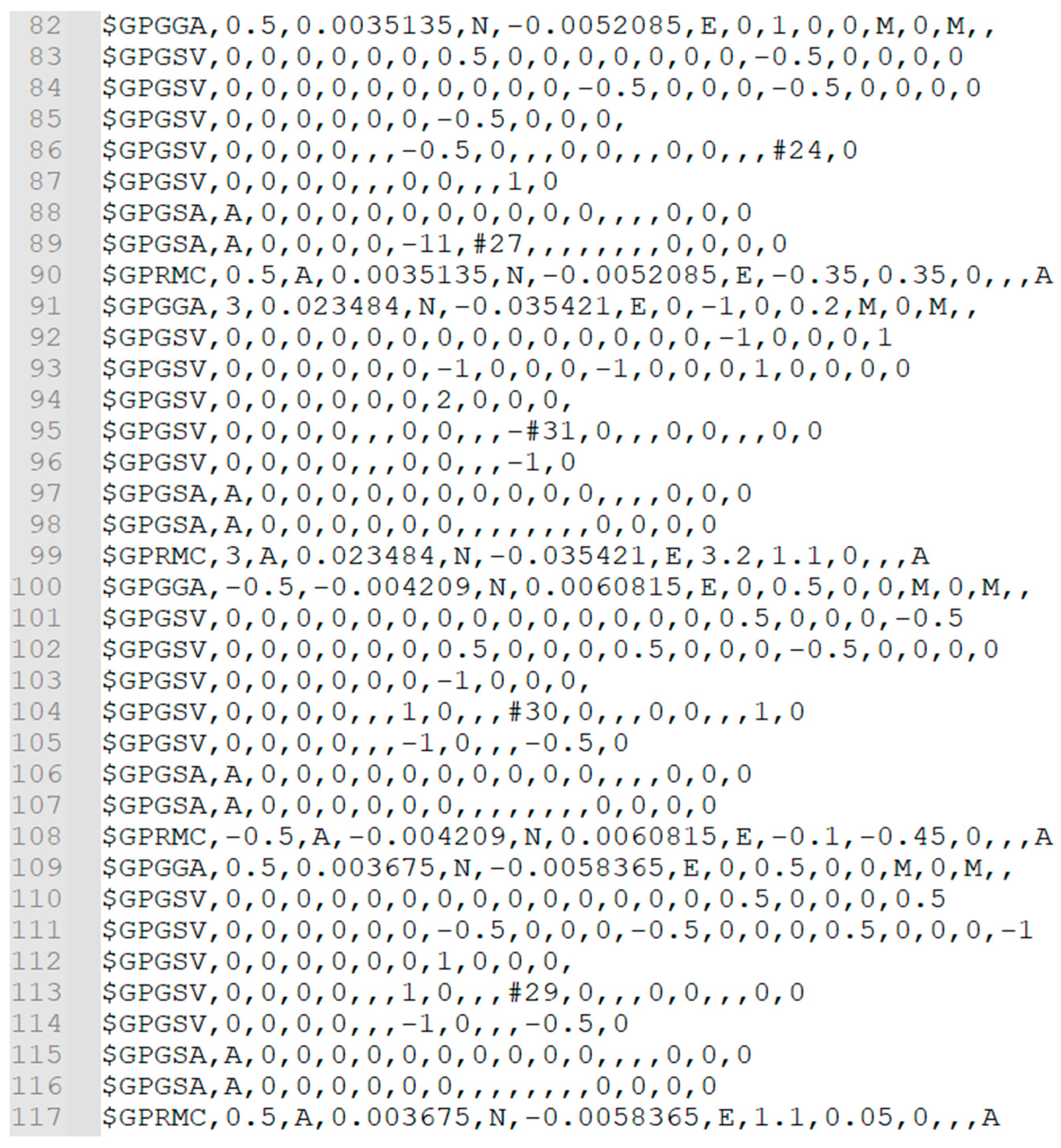
An example of the different file is shown in Figure A6 in Appendix A.
- After receiving the different file in Figure A6 in Appendix A, the algorithm prepares a file that contains very long prefixes that usually repeat in various files. Our algorithm maps each of these prefixes with a distinct symbol.
- The algorithm takes the output file from step 1 and executes a mapping file, creating a Huffman encoding for the file from step 1.
A simulation program was built for compression and decompression in C#. This tool tests and calculates different compression, coding, and decoding methods.
A diagram illustrating the compression is in Figure 3.
We developed simulation software to implement the suggestions of this work. The interface of the simulation program is shown in Figure 4.
This simulator is given a raw GNSS data file. The course of action is:
- For encoding:
- Load text file (GNSS logs).
- Create a difference file based on the H.264-like algorithm.
- For first run:
- Generate prefix configuration file.
- From a mapping file.
- Produce Huffman configuration file.
- Execute Huffman coding algorithm (creates .bin file)
- For decoding:
- e.
- Load Huffman coding file (the .bin file)
- f.
- Decode bin file using Huffman algorithm.
- g.
- Execute reversed difference file based on the H.264-like algorithm.
7. Results
This compression method contains three steps:
- The difference method is based on H.264.
- Mapping.
- Huffman coding.
One of the significant advantages of this compression method (compared to zip compression) is that ours has error resilience because of the Huffman Codes [5].
ZIP does not have this attribute of error resilience, and it is almost impossible to recover damaged files. In addition, if the files using ZIP were sent in parts and one part were not received, then the information could not be recovered at all [57].
In each message transmission using the method proposed in this paper, we send a first packet that is always original and without any changes. Therefore, because of this feature, we recover the subsequent packets.
If some of the packages are lost, because of the Huffman property of synchronization, we would recover the rest of the information at a relatively high speed. In addition, the first packet is transmitted at a certain frequency each time the number of messages in the GPGSV protocol changes.
Therefore, when there is a change in the GPGSV protocol, the existing file is closed, and a new file is opened in a renewed procedure, and thus we create additional error resilience to information loss due to the repeatability of the first package.
This durability does not exist in the Zip compression method (not in real time). If some of the information does not arrive or goes wrong in transmission, ZIP will not be able even partially to restore the information. The suggested method of compression has been evaluated by several benchmark tests employing real GNSS information obtained from the GNSS of real vehicles. We tried Zip as it is, as well as Diff’ the method employing the concept of H.264 described above. The output of Diff was sent to Huffman, Zip, and a mapping of repeated strings before doing the Zip.
We have marked in bold in the following tables the method we propose in this study, the winning method among all those tested and reviewed. The results of the first benchmark are detailed in Table 1 (GNSS data file and compression results).
In the next results, we will be able to see a slight improvement with larger files, but at a certain stage, the improvement is not significant, and the results remain about the same numbers.
We see that after calculating and using the difference method (Diff file), which is a preprocessing stage, we get a reduction of 28%. The significant gain is not just the gain of 28% but the number of zeros we get after the differences. These help us to compress the information more efficiently using the Huffman code and achieving better significant compression percentages.
After using the difference method, which is a preprocessor for Huffman coding, we will get a significantly better compression ratio (compared to the original file), of about 87%.Nevertheless, if we want to improve and compete with ZIP, first we perform the difference method, which preprocesses for Huffman, and then directly apply ZIP compression and thus get a better compression percentage of about 91.3% compared to about 90% by directly using ZIP on an original file
Furthermore, it is possible to compress even better after performing the difference method, then using the mapping method, and then Zip; the result is significantly better—93.4%.
Naturally, we must take into account that the world is not perfect and sometimes successes come at the expense of something else. The high compression rates we get here, which are better than with Zip, come at the expense of not being able to recover if the file or parts of it are damaged during transmitting or building (survivability).
We also tried some larger files, and the results were a little bit better. The results of the larger files can be found in Table 2 (GNSS data file and compression results).
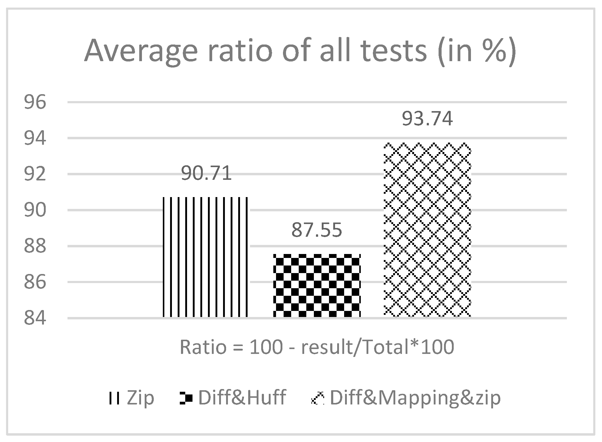
Figure 5 compares the average percentages of size that have been saved by each of the methods. It can be concluded that Diff&Mapping&Zip gives the best compression, but there is no error resilience in this method, whereas Diff&Huffman, even with somewhat lower results, has the feature of automatic error resilience.
Another option that has been tested is performing ZIP compression and then running compression using our algorithm. This option was ruled out because after doing ZIP, a file that is mostly random will be created, and random files cannot be compressed [58].
Huffman coding is a very popular method used by many applications such as MP3 and JPEG. At the same time, another method can be used—that of Shannon Fano [59], but its compression is inferior to Huffman coding [60]. Therefore, we preferred Huffman codes.
In the table in Appendix B, we see how many bits we save per symbol by using Huffman codes. However, we save even more because the compression method presented here has several stages, so in the preliminary stage we have already converted a sequence of repeating characters (prefixes) into one symbol and have already made some reduction in the data size.
To evaluate the efficiency of the proposed method, we calculate Shannon Entropy. Shannon Entropy Formula is where is the probability of getting the value . More explanation of the Shannon Entropy formula can be found in [61].
It can be seen in the detailed spreadsheet in Appendix B that Shannon’s entropy gives a result of 5.548, which is indeed optimal. This entropy is very close to the result obtained in this work by using Huffman coding 5.581. The results are shown in Figure 6.
The slight increment occurs because the Huffman algorithm rounds off the number of bits for each codeword and therefore a very close entropy is obtained by the Huffman algorithm, even if not optimal.
8. Conclusions
Several compression methods as well as a combination of different compression methods and their results have been presented. Compression using only Zip is about a saving of 90%. This is undoubtedly a substantial compression ratio, but unfortunately with quite a few shortcomings as noted in this work.
It is possible to compress with a full method as suggested in this research and obtain a reduction of over 87% of all the raw information. Considering the good error resilience because of Huffman and sometimes sending raw information, it can be concluded that there is an evident trade-off here with a cost of about 3% compared to ZIP.
A better compression ratio can be obtained by combining part of the method developed in this paper and then performing compression by ZIP. This algorithm outperforms the two previous and obtains a data reduction of about 94% (3% better than ZIP and 6% better than the Huffman-based method which we suggested here). Nevertheless, it should be noted that in the combined method, there is no good error resilience because Huffman Coding is not used.
Our choice and recommendation are to use the difference method together with Huffman rather than a pure ZIP method or other combinations that we mentioned above. We prefer the difference method together with Huffman because the other methods do not provide error resilience, even though they can slightly improve the compression ratio.
It should also be noted that during the coding, we used static and not dynamic coding tables. This feature has pros and cons. It is common to have a static and known table in advance, because this is efficient and saves the need to update and transfer the compression tables. Everyone has the known tables and there is no need that the transferred information to include new tables each time. Yet, a custom table can generate a shorter average code-word. Therefore, we chose to use static tables as customary in most compression methods such as JPEG, TIFF, MP3 and more.
We believe that using the methods presented in this paper can significantly improve the efficiency and speed of information transfer. This is particularly important nowadays since there is no use of NMEA data compression in GNSSes and not enough research and work has been done on this subject. Therefore, further attention should be given to NMEA raw data that is currently transmitted uncompressed. In a future study, we suggest checking how to improve the compression and reach optimal results by using alternative codes for Huffman’s. Other methods that can be used without rounding the bits up like Arithmetic Coding should be considered. Also, a possibility of adding error resilience and/or error checking like checksum to the more efficient zip methods presented here (Diff&Mapping&Zip) can be considered.
The Huffman code synchronizes after an error with almost 100% probability. That is, after several wrong code words, the Huffman algorithm automatically comes back to itself and starts reading real code words. In contrast, arithmetic coding does not synchronize after an error and all the data that is read and decoded after the error is wrong. The proposal to work with arithmetic coding improves the compression percentages, but it comes at the cost of no synchronization after an error, so a mechanism for synchronization after errors such as a checksum may possibly be considered.
We also suggest considering in advance the possibility of not transmitting unchanged information in relation to the previous information (for example, if the vehicle is stopped at traffic lights or in a traffic jam).
Author Contributions
Conceptualization, Y.W. and A.R.; methodology, A.R.; software, A.R.; validation, A.R.; formal analysis, A.R. and Y.W.; investigation, A.R.; resources, A.R.; data curation, A.R.; writing—original draft preparation, A.R.; writing—review and editing, A.R. and Y.W.; supervision, Y.W.; project administration, A.R. and Y.W.; All authors have read and agreed to the published version of the manuscript.
Funding
This research received no external funding.
Data Availability Statement
Not applicable.
Acknowledgments
We are very grateful to all those who contributed to the success of this research. First and foremost, we would like to thank Eduard Yakubov and Eugen Mandrescu for all their support and encouragement throughout the process of research. Also, we would like to express our gratitude to Radel Ben-Av, who provided valuable information, insights and assistance with his extensive experience in the field. In addition, many thanks to my good friend Alrajoub Eyas for his contribution in supporting the development of tools that were very important to the success of this research, and we are grateful for his intense and dedicated help.
Conflicts of Interest
The authors declare no conflict of interest.
Appendix A
Figure A1.
Untouched file from NMEA Logger before filtering.

Figure A2.
File after filtering.

Figure A3.
Example of incorrect information in a database.

Figure A4.
Case with different number of GPGSV lines.

Figure A5.
Different fields in the same type of line.

Figure A6.
Difference file (Diff file).

Appendix B
This spreadsheet is a static conversion table for each symbol. This table also shows the occurrence frequency of each symbol and its Huffman coding. We can see in addition in this table how much per-symbol space we were able to save and an entropy calculation in relation to the per-character average.
Average bits per symbol is 5.5814.
Entropy is 5.5481.

Table A1.
Fixed character encoding and decoding map used in this study.
| Symbols | Frequency | Huffman Coding | Num of Bits | Space Savings (Bits) | Saved Bits | Freq × Num of Bits | Entropy |
|---|---|---|---|---|---|---|---|
| 0 | 193,868 | 010 | 3 | 193,868 × 8 − 193,868 × 3 = 969,340 | 969,340 | 581,604 | 0.3401972807 |
| % | 128,388 | 1011 | 4 | 128,388 × 8 − 128,388 × 4 = 513,552 | 513,552 | 513,552 | 0.2663735204 |
| - | 97,393 | 0110 | 4 | 97,393 × 8 − 97,393 × 4 = 389,572 | 389,572 | 389,572 | 0.2229590946 |
| 1 | 91,188 | 0010 | 4 | 91,188 × 8 − 91,188 × 4 = 364,752 | 364,752 | 364,752 | 0.2134148223 |
| , | 82,150 | 11110 | 5 | 82,150 × 8 − 82,150 × 5 = 246,450 | 246,450 | 410,750 | 0.1989196096 |
| ¦ | 81,703 | 11101 | 5 | 81,703 × 8 − 81,703 × 5 = 245,109 | 245,109 | 408,515 | 0.1981833350 |
| © | 74,786 | 11010 | 5 | 74,786 × 8 − 74,786 × 5 = 224,358 | 224,358 | 373,930 | 0.1865413311 |
| 2 | 61,997 | 10011 | 5 | 61,997 × 8 − 61,997 × 5 = 185,991 | 185,991 | 309,985 | 0.1636685171 |
| 5 | 52,276 | 10000 | 5 | 52,276 × 8 − 52,276 × 5 = 156,828 | 156,828 | 261,380 | 0.1449276078 |
| 3 | 49,158 | 01110 | 5 | 49,158 × 8 − 49,158 × 5 = 147,474 | 147,474 | 245,790 | 0.1386305132 |
| y | 41,594 | 111110 | 6 | 41,594 × 8 − 41,594 × 6 = 83,188 | 83,188 | 249,564 | 0.1226949237 |
| < | 38,094 | 111000 | 6 | 38,094 × 8 − 38,094 × 6 = 76,188 | 76,188 | 228,564 | 0.1149702278 |
| I | 35,174 | 110010 | 6 | 35,174 × 8 − 35,174 × 6 = 70,348 | 70,348 | 211,044 | 0.1083353318 |
| F | 35,146 | 110001 | 6 | 35,146 × 8 − 35,146 × 6 = 70,292 | 70,292 | 210,876 | 0.1082708225 |
| > | 31,515 | 101001 | 6 | 31,515 × 8 − 31,515 × 6 = 63,030 | 63,030 | 189,090 | 0.0997533134 |
| 4 | 29,563 | 100101 | 6 | 29,563 × 8 − 29,563 × 6 = 59,126 | 59,126 | 177,378 | 0.0950422933 |
| r | 27,118 | 100010 | 6 | 27,118 × 8 − 27,118 × 6 = 54,236 | 54,236 | 162,708 | 0.0889993603 |
| § | 26,345 | 011111 | 6 | 26,345 × 8 − 26,345 × 6 = 52,690 | 52,690 | 158,070 | 0.0870539414 |
| 6 | 25,197 | 011110 | 6 | 25,197 × 8 − 25,197 × 6 = 50,394 | 50,394 | 151,182 | 0.0841320976 |
| ^ | 24,585 | 001111 | 6 | 24,585 × 8 − 24,585 × 6 = 49,170 | 49,170 | 147,510 | 0.0825579785 |
| # | 24,135 | 001101 | 6 | 24,135 × 8 − 24,135 × 6 = 48,270 | 48,270 | 144,810 | 0.0813930080 |
| ¤ | 23,174 | 001100 | 6 | 23,174 × 8 − 23,174 × 6 = 46,348 | 46,348 | 139,044 | 0.0788831806 |
| 9 | 22,641 | 000110 | 6 | 22,641 × 8 − 22,641 × 6 = 45,282 | 45,282 | 135,846 | 0.0774778937 |
| 7 | 22,606 | 000101 | 6 | 22,606 × 8 − 22,606 × 6 = 45,212 | 45,212 | 135,636 | 0.0773852757 |
| } | 22,419 | 000011 | 6 | 22,419 × 8 − 22,419 × 6 = 44,838 | 44,838 | 134,514 | 0.0768897164 |
| * | 22,347 | 000010 | 6 | 22,347 × 8 − 22,347 × 6 = 44,694 | 44,694 | 134,082 | 0.0766985905 |
| @ | 22,144 | 000001 | 6 | 22,144 × 8 − 22,144 × 6 = 44,288 | 44,288 | 132,864 | 0.0761587499 |
| 8 | 21,345 | 1111111 | 7 | 21,345 × 8 − 21,345 × 7 = 21,345 | 21,345 | 149,415 | 0.0740197954 |
| v | 19,685 | 1110010 | 7 | 19,685 × 8 − 19,685 × 7 = 19,685 | 19,685 | 137,795 | 0.0695006163 |
| t | 18,883 | 1101110 | 7 | 18,883 × 8 − 18,883 × 7 = 18,883 | 18,883 | 132,181 | 0.0672788481 |
| ú | 18,839 | 1101101 | 7 | 18,839 × 8 − 18,839 × 7 = 18,839 | 18,839 | 131,873 | 0.0671562004 |
| x | 18,544 | 1101100 | 7 | 18,544 × 8 − 18,544 × 7 = 18,544 | 18,544 | 129,808 | 0.0663318331 |
| ( | 17,649 | 1100110 | 7 | 17,649 × 8 − 17,649 × 7 = 17,649 | 17,649 | 123,543 | 0.0638082439 |
| ‘ | 16,978 | 1100000 | 7 | 16,978 × 8 − 16,978 × 7 = 16,978 | 16,978 | 118,846 | 0.0618932344 |
| ô | 16,539 | 1010110 | 7 | 16,539 × 8 − 16,539 × 7 = 16,539 | 16,539 | 115,773 | 0.0606292513 |
| ¿ | 15,878 | 1010101 | 7 | 15,878 × 8 − 158,78 × 7 = 15,878 | 15,878 | 111,146 | 0.0587089325 |
| ¾ | 15,584 | 1010001 | 7 | 15,584 × 8 − 15,584 × 7 = 15,584 | 15,584 | 109,088 | 0.0578479990 |
| X | 15,133 | 1010000 | 7 | 15,133 × 8 − 15,133 × 7 = 15,133 | 15,133 | 105,931 | 0.0565189165 |
| Â | 14,659 | 1001001 | 7 | 14,659 × 8 − 14,659 × 7 = 14,659 | 14,659 | 102,613 | 0.0551107992 |
| E | 14,002 | 1000111 | 7 | 14,002 × 8 − 14,002 × 7 = 14,002 | 14,002 | 98,014 | 0.0531392767 |
| | | 11,595 | 0001111 | 7 | 11,595 × 8 − 11,595 × 7 = 11,595 | 11,595 | 81,165 | 0.0457024780 |
| u | 11,549 | 0001110 | 7 | 11,549 × 8 − 11,549 × 7 = 11,549 | 11,549 | 80,843 | 0.0455568088 |
| ± | 11,140 | 0001000 | 7 | 11,140 × 8 − 11,140 × 7 = 11,140 | 11,140 | 77,980 | 0.0442552980 |
| z | 10,792 | 0000000 | 7 | 10,792 × 8 − 10,792 × 7 = 10,792 | 10,792 | 75,544 | 0.0431387351 |
| / | 10,575 | 11111101 | 8 | 10,575 × 8 − 10,575 × 8 = 0 | 0 | 84,600 | 0.0424380946 |
| ¥ | 10,471 | 11111100 | 8 | 10,471 × 8 − 10,471 × 8 = 0 | 0 | 83,768 | 0.0421010826 |
| . | 9949 | 11100110 | 8 | 9949 × 8 − 9949 × 8 = 0 | 0 | 79,592 | 0.0403972615 |
| û | 9833 | 11011111 | 8 | 9833 × 8 − 9833 × 8 = 0 | 0 | 78,664 | 0.0400157852 |
| ä | 9040 | 11001111 | 8 | 9040 × 8 − 9040 × 8 = 0 | 0 | 72,320 | 0.0373787946 |
| ) | 8945 | 11001110 | 8 | 8945 × 8 − 8945 × 8 = 0 | 0 | 71,560 | 0.0370593545 |
| é | 8514 | 11000011 | 8 | 8514 × 8 − 8514 × 8 = 0 | 0 | 68,112 | 0.0356001401 |
| _ | 8466 | 11000010 | 8 | 8466 × 8 − 8466 × 8 = 0 | 0 | 67,728 | 0.0354365961 |
| s | 8130 | 10101001 | 8 | 8130 × 8 − 8130 × 8 = 0 | 0 | 65,040 | 0.0342858027 |
| ½ | 7315 | 10010001 | 8 | 7315 × 8 − 7315 × 8 = 0 | 0 | 58,520 | 0.0314487129 |
| Š | 6900 | 10001101 | 8 | 6900 × 8 − 6900 × 8 = 0 | 0 | 55,200 | 0.0299774250 |
| U | 5907 | 00111000 | 8 | 5907 × 8 − 5907 × 8 = 0 | 0 | 47,256 | 0.0263758905 |
| ~ | 5459 | 00000011 | 8 | 5459 × 8 − 5459 × 8 = 0 | 0 | 43,672 | 0.0247097701 |
| î | 5024 | 111001110 | 9 | 5024 × 8 − 5024 × 9 = −5024 | −5024 | 45,216 | 0.0230646747 |
| « | 4314 | 101011111 | 9 | 4314 × 8 − 4314 × 9 = −4314 | −4314 | 38,826 | 0.0203154453 |
| þ | 4142 | 101011110 | 9 | 4142 × 8 − 4142 × 9 = −4142 | −4142 | 37,278 | 0.0196363053 |
| œ | 4106 | 101011101 | 9 | 4106 × 8 − 4106 × 9 = −4106 | −4106 | 36,954 | 0.0194934655 |
| ï | 3857 | 101010001 | 9 | 3857 × 8 − 3857 × 9 = −3857 | −3857 | 34,713 | 0.0184986608 |
| + | 3636 | 100100000 | 9 | 3636 × 8 − 3636 × 9 = −3636 | −3636 | 32,724 | 0.0176052864 |
| w | 3229 | 001110111 | 9 | 3229 × 8 − 3229 × 9 = −3229 | −3229 | 29,061 | 0.0159322230 |
| ç | 3089 | 001110110 | 9 | 3089 × 8 − 3089 × 9 = −3089 | −3089 | 27,801 | 0.0153477517 |
| ¬ | 3062 | 001110101 | 9 | 3062 × 8 − 3062 × 9 = −3062 | −3062 | 27,558 | 0.0152344723 |
| p | 3024 | 001110011 | 9 | 3024 × 8 − 3024 × 9 = −3024 | −3024 | 27,216 | 0.0150747286 |
| q | 2818 | 000100110 | 9 | 2818 × 8 − 2818 × 9 = −2818 | −2818 | 25,362 | 0.0142021730 |
| ñ | 2796 | 000100100 | 9 | 2796 × 8 − 2796 × 9 = −2796 | −2796 | 25,164 | 0.0141083110 |
| ê | 2665 | 000000100 | 9 | 2665 × 8 − 2665 × 9 = −2665 | −2665 | 23,985 | 0.0135465855 |
| D | 2600 | 1110011111 | 10 | 2600 × 8 − 2600 × 10 = −5200 | −5200 | 26,000 | 0.0132660257 |
| ö | 2583 | 1110011110 | 10 | 2583 × 8 − 2583 × 10 = −5166 | −5166 | 25,830 | 0.0131924417 |
| K | 2344 | 1101111010 | 10 | 2344 × 8 − 2344 × 10 = −4688 | −4688 | 23,440 | 0.0121484651 |
| Á | 2310 | 1101111001 | 10 | 2310 × 8 − 2310 × 10 = −4620 | −4620 | 23,100 | 0.0119984550 |
| ¶ | 2160 | 1101111000 | 10 | 2160 × 8 − 2160 × 10 = −4320 | −4320 | 21,600 | 0.0113319272 |
| m | 2002 | 1010111000 | 10 | 2002 × 8 − 2002 × 10 = −4004 | −4004 | 20,020 | 0.0106210870 |
| f | 1867 | 1010100000 | 10 | 1867 × 8 − 1867 × 10 = −3734 | −3734 | 18,670 | 0.0100060762 |
| õ | 1840 | 1001000011 | 10 | 1840 × 8 − 1840 × 10 = −3680 | −3680 | 18,400 | 0.0098821815 |
| Q | 1665 | 1000110001 | 10 | 1665 × 8 − 1665 × 10 = −3330 | −3330 | 16,650 | 0.0090714919 |
| o | 1531 | 0011101001 | 10 | 1531 × 8 − 1531 × 10 = −3062 | −3062 | 15,310 | 0.0084411465 |
| ð | 1528 | 0011101000 | 10 | 1528 × 8 − 1528 × 10 = −3056 | −3056 | 15,280 | 0.0084269329 |
| e | 1509 | 0011100101 | 10 | 1509 × 8 − 1509 × 10 = −3018 | −3018 | 15,090 | 0.0083368070 |
| Ì | 1469 | 0011100100 | 10 | 1469 × 8 − 1469 × 10 = −2938 | −2938 | 14,690 | 0.0081464584 |
| ø | 1428 | 0001001110 | 10 | 1428 × 8 − 1428 × 10 = −2856 | −2856 | 14,280 | 0.0079504731 |
| ® | 1415 | 0001001011 | 10 | 1415 × 8 − 1415 × 10 = −2830 | −2830 | 14,150 | 0.0078881418 |
| J | 1365 | 0000001011 | 10 | 1365 × 8 − 1365 × 10 = −2730 | −2730 | 13,650 | 0.0076475342 |
| n | 1330 | 11011110111 | 11 | 1330 × 8 − 1330 × 11 = −3990 | −3990 | 14,630 | 0.0074782658 |
| i | 1040 | 10101110011 | 11 | 1040 × 8 − 1040 × 11 = −3120 | −3120 | 11,440 | 0.0060462641 |
| k | 1019 | 10101000011 | 11 | 1019 × 8 − 1019 × 11 = −3057 | −3057 | 11,209 | 0.0059403145 |
| l | 929 | 10010000101 | 11 | 929 × 8 − 929 × 11 = −2787 | −2787 | 10,219 | 0.0054823489 |
| j | 906 | 10010000100 | 11 | 906 × 8 − 906 × 11 = −2718 | −2718 | 9966 | 0.0053642520 |
| Ž | 898 | 10001100111 | 11 | 898 × 8 − 898 × 11 = −2694 | −2694 | 9878 | 0.0053230692 |
| Œ | 895 | 10001100110 | 11 | 895 × 8 − 895 × 11 = −2685 | −2685 | 9845 | 0.0053076114 |
| ? | 893 | 10001100101 | 11 | 893 × 8 − 893 × 11 = −2679 | −2679 | 9823 | 0.0052973018 |
| N | 884 | 10001100100 | 11 | 884 × 8 − 884 × 11 = −2652 | −2652 | 9724 | 0.0052508657 |
| í | 812 | 10001100000 | 11 | 812 × 8 − 812 × 11 = −2436 | −2436 | 8932 | 0.0048767525 |
| Space | 724 | 00010011110 | 11 | 724 × 8 − 724 × 11 = −2172 | −2172 | 7964 | 0.0044127160 |
| a | 709 | 00010010101 | 11 | 709 × 8 − 709 × 11 = −2127 | −2127 | 7799 | 0.0043328166 |
| g | 679 | 00000010101 | 11 | 679 × 8 − 679 × 11 = −2037 | −2037 | 7469 | 0.0041722735 |
| µ | 659 | 00000010100 | 11 | 659 × 8 − 659 × 11 = −1977 | −1977 | 7249 | 0.0040646756 |
| ß | 616 | 110111101101 | 12 | 616 × 8 − 616 × 12 = −2464 | −2464 | 7392 | 0.0038317250 |
| ÿ | 607 | 110111101100 | 12 | 607 × 8 − 607 × 12 = −2428 | −2428 | 7284 | 0.0037826782 |
| T | 520 | 101011100101 | 12 | 520 × 8 − 520 × 12 = −2080 | −2080 | 6240 | 0.0033029709 |
| ü | 495 | 101010000101 | 12 | 495 × 8 − 495 × 12 = −1980 | −1980 | 5940 | 0.0031631097 |
| M | 444 | 101010000100 | 12 | 444 × 8 − 444 × 12 = −1776 | −1776 | 5328 | 0.0028746957 |
| ó | 402 | 100011000010 | 12 | 402 × 8 − 402 × 12 = −1608 | −1608 | 4824 | 0.0026337800 |
| b | 352 | 000100111110 | 12 | 352 × 8 − 352 × 12 = −1408 | −1408 | 4224 | 0.0023424939 |
| L | 345 | 000100101001 | 12 | 345 × 8 − 345 × 12 = −1380 | −1380 | 4140 | 0.0023012906 |
| O | 345 | 000100101000 | 12 | 345 × 8 − 345 × 12 = −1380 | −1380 | 4140 | 0.0023012906 |
| Z | 293 | 1010111001001 | 13 | 293 × 8 − 293 × 13 = −1465 | −1465 | 3809 | 0.0019915935 |
| æ | 223 | 1010111001000 | 13 | 223 × 8 − 223 × 13 = −1115 | −1115 | 2899 | 0.0015630521 |
| c | 221 | 1000110000111 | 13 | 221 × 8 − 221 × 13 = −1105 | −1105 | 2873 | 0.0015505795 |
| Y | 219 | 1000110000110 | 13 | 219 × 8 − 219 × 13 = −1095 | −1095 | 2847 | 0.0015380928 |
| ë | 186 | 0001001111110 | 13 | 186 × 8 − 186 × 13 = −930 | −930 | 2418 | 0.0013299109 |
| ù | 92 | 00010011111110 | 14 | 92 × 8 − 92 × 14 = −552 | −552 | 1288 | 0.0007080876 |
| £ | 62 | 000100111111111 | 15 | 62 × 8 − 62 × 15 = −434 | −434 | 930 | 0.0004961866 |
| € | 32 | 0001001111111101 | 16 | 32 × 8 − 32 × 16 = −256 | −256 | 512 | 0.0002725284 |
| Í | 1 | 0001001111111100 | 16 | 1 × 8 − 1 × 16 = −8 | −8 | 16 | 0.0000112073 |
| Total freq: 1,858,212 | Saved bits: 4,494,225 | 10,371,471 | Entropy: 5.5481 |
References
- Raviteja, T.; Vedaraj, I.R. An Introduction of autonomous vehicles and A brief survey. J. Crit. Rev. 2020, 7, 13. [Google Scholar]
- Wiseman, Y. Autonomous Vehicles. In Encyclopedia of Information Science and Technology, 5th ed.; IGI Global: Hershey, PA, USA, 2020; Volume 1, Chapter 1; pp. 1–11. [Google Scholar]
- Parekh, D.; Poddar, N.; Rajpurkar, A.; Chahal, M.; Kumar, N.; Joshi, G.P.; Cho, W. A review on autonomous vehicles: Progress, methods and challenges. Electronics 2022, 11, 2162. [Google Scholar] [CrossRef]
- Cosgun, A.; Ma, L.; Chiu, J.; Huang, J.; Demir, M.; Anon, A.M.; Lian, T.; Tafish, H.; Al-Stouhi, S. Towards full automated drive in urban environments: A demonstration in GoMentum Station, California. In Proceedings of the 2017 IEEE Intelligent Vehicles Symposium (IV), Los Angeles, CA, USA, 11–14 June 2017; IEEE: Piscataway, NJ, USA, 2017. [Google Scholar]
- Klein, S.T.; Wiseman, Y. Parallel Huffman Decoding with Applications to JPEG Files. Comput. J. 2003, 46, 487–497. [Google Scholar] [CrossRef]
- Krile, S.; Kezić, D.; Dimc, F. NMEA Communication Standard for Shipboard Data Architecture. NAŠE MORE Znan. Časopis More Pomor. 2013, 60, 68–81. [Google Scholar]
- Marcellin, M.W.; Gormish, M.J.; Bilgin, A.; Boliek, M.P. An overview of JPEG-2000. In Proceedings of the DCC 2000. Data Compression Conference, Snowbird, UT, USA, 28–30 March 2000; IEEE: Piscataway, NJ, USA, 2000. [Google Scholar]
- Nurrohman, A.; Abdurohman, M. High performance streaming based on H264 and real time messaging protocol (RTMP). In Proceedings of the 2018 6th International Conference on Information and Communication Technology (ICoICT), Bandung, Indonesia, 3–5 May 2018; IEEE: Piscataway, NJ, USA, 2018. [Google Scholar]
- Chen, J.W.; Kao, C.Y.; Lin, Y.L. Introduction to H. 264 advanced video coding. In Proceedings of the 2006 Asia and South Pacific Design Automation Conference, Yokohama, Japan, 24–27 January 2006. [Google Scholar]
- Taeihagh, A.; Lim, H.S.M. Governing autonomous vehicles: Emerging responses for safety, liability, privacy, cybersecurity, and industry risks. Transp. Rev. 2019, 39, 103–128. [Google Scholar] [CrossRef]
- Hacohen, S.; Medina, O. Autonomous Vehicle, Sensing and Communication Survey; Ariel University: Ariel, Israel, 2020. [Google Scholar]
- UK Government. The Key Principles of Vehicle Cyber Security for Connected and Automated Vehicles; Centre for Connected and Autonomous Vehicles, Department for Transport Guidance: London, UK, 2017.
- Fitriya, L.A.; Purboyo, T.W.; Prasasti, A.L. A Review of Data Compression Techniques. Int. J. Appl. Eng. Res. 2017, 12, 19. [Google Scholar]
- Svanberg, J.; Palmkvist, K. Lightweight Real-Time Lossless Software Compression of Trace Data. Master’s Thesis, Department of Electrical Engineering, Linköping University, Linköping, Sweden, 2021. [Google Scholar]
- Huffman, D.A. A Method for the Construction of Minimum-Redundancy Codes. Proc. IRE 1952, 40, 1098–1101. [Google Scholar] [CrossRef]
- Alistair, M. Huffman Coding. ACM Comput. Surv. 2019, 52, 4. [Google Scholar]
- Hashemian, R. Memory efficient and high-speed search Huffman coding. IEEE Trans. Commun. 1995, 43, 2576–2581. [Google Scholar] [CrossRef]
- Shen, L.; Stopher, P.R. Review of GPS Travel Survey and GPS Data-Processing Methods. Transp. Rev. 2014, 34, 316–334. [Google Scholar] [CrossRef]
- Abulude, F.; Akinnusotu, A.; Adeyemi, A. Global Positioning System and Its Wide Applications. Wilolud J. 2015, 9, 22–30. [Google Scholar]
- Curry, A. The internet of Animals. Nature 2018, 562, 322–326. [Google Scholar] [CrossRef] [PubMed]
- Martin, B. Technology to the Rescue. In Survival or Extinction? Springer: Berlin/Heidelberg, Germany, 2019; pp. 319–330. [Google Scholar]
- Buchheit, M.; Al Haddad, H.; Simpson, B.M.; Palazzi, D.; Bourdon, P.C.; Di Salvo, V.; Mendez-Villanueva, A. Monitoring Accelerations with GPS in Football: Time to Slow Down? Int. J. Sports Physiol. Perform. 2014, 9, 442–445. [Google Scholar] [CrossRef]
- Rahiman, W.; Zainal, Z. An Overview of Development GPS Navigation for Autonomous Car. In Proceedings of the 2013 IEEE 8th Conference on Industrial Electronics and Applications (ICIEA), Melbourne, Australia, 19–21 June 2013; IEEE: Piscataway, NJ, USA, 2013; pp. 1112–1118. [Google Scholar]
- Mathiesen, T.T. GPS, NMEA, WGS-84, GIS and VB.NET. Available online: http://www.tma.dk/gps/ (accessed on 16 July 2008).
- Langley, R. Nmea 0183: A gps receiver. GPS World 1995, 6, 54–57. [Google Scholar]
- Si, H.; Aung, Z.M. Position Data Acquisition from NMEA Protocol of Global Positioning System. Int. J. Comput. Electr. Eng. 2011, 3, 353–357. [Google Scholar] [CrossRef]
- Lever, R.; Hinze, A.; Buchanan, G. Compressing gps data on mobile devices. In On the Move to Meaningful Internet Systems 2006: OTM 2006 Workshops: OTM Confederated International Workshops and Posters, AWeSOMe, CAMS, COMINF, IS, KSinBIT, MIOS-CIAO, MONET, OnToContent, ORM, PerSys, OTM Academy Doc-Toral Consortium, RDDS, SWWS, and SeBGIS 2006, Montpellier, France, 29 October–3 November 2006; Proceedings, Part II; Springer: Berlin/Heidelberg, Germany, 2006. [Google Scholar]
- DePriest, D. NMEA Data. Available online: https://web.fe.up.pt/~ee95080/NMEA%20data.pdf (accessed on 16 August 2021).
- Novatel, H. GNSS Logs. 2022. Available online: https://docs.novatel.com/OEM7/Content/Logs/Core_Logs.htm (accessed on 16 August 2021).
- Rahnamai, K.; Gorman, K.; Gray, A.; Arabshahi, P. Formations of Autonomous Vehicles Using Global Positioning Systems (GPS). In Proceedings of the 2005 IEEE Aerospace Conference, Big Sky, Montana, 5–12 March 2005; IEEE: Piscataway, NJ, USA, 2005. [Google Scholar]
- Ulku, E.E.; Bekmezci, I. Multi token based location sharing for multi UAV systems. Int. J. Comput. Electr. Eng. 2016, 8, 197. [Google Scholar] [CrossRef]
- Kakad, S.; Sarode, P.; Bakal, J.W. A survey on query response time optimization approaches for reliable data communication in wireless sensor network. Int. J. Wirel. Commun. Netw. Technol. 2012, 1, 31–36. [Google Scholar]
- Jurdana, I.; Lopac, N.; Wakabayashi, N.; Liu, H. Shipboard Data Compression Method for Sustainable Real-Time Maritime Communication in Remote Voyage Monitoring of Autonomous Ships. Sustainability 2021, 13, 8264. [Google Scholar] [CrossRef]
- Kabir, M.; Kang, M.J.; Wu, X.; Hamidi, M. Study on U-turn behavior of vessels in narrow waterways based on AIS data. Ocean Eng. 2022, 246, 110608. [Google Scholar] [CrossRef]
- Correia, S.D.; Perez, R.; Matos-Carvalho, J.; Leithardt, V.R.Q. μJSON, a Lightweight Compression Scheme for Embedded GNSS Data Transmission on IoT Nodes. In Proceedings of the 2022 5th Conference on Cloud and Internet of Things (CIoT), Marrakech, Morocco, 28–30 March 2022; IEEE: Piscataway, NJ, USA, 2022. [Google Scholar]
- Zhou, F.; Zhao, L.; Li, L.; Hu, Y.; Jiang, X.; Yu, J.; Liang, G. GNSS Signal Acquisition Algorithm Based on Two-Stage Compression of Code-Frequency Domain. Appl. Sci. 2022, 12, 6255. [Google Scholar] [CrossRef]
- Ansari, B.; Kaushik, V.; Biswas, S.K. Raw GNSS Data Compression using Compressive Sensing for Reflectometry Applications. In Proceedings of the 2020 XXXIIIrd General Assembly and Scientific Symposium of the International Union of Radio Science, Rome, Italy, 29 August–5 September 2020; IEEE: Piscataway, NJ, USA, 2020. [Google Scholar]
- Perez, R.; Leithardt, V.R.Q.; Correia, S.D. Lossless Compression Scheme for Efficient GNSS Data Transmission on IoT Devices. In Proceedings of the 2021 International Conference on Electrical, Computer and Energy Technologies (ICECET), Cape Town, South Africa, 9–10 December 2021; IEEE: Piscataway, NJ, USA, 2021. [Google Scholar]
- Muckell, J.; Hwang, J.H.; Patil, V.; Lawson, C.T.; Ping, F.; Ravi, S.S. SQUISH: An online approach for GPS trajectory compression. In Proceedings of the 2nd International Conference on Computing for Geospatial Research & Applications, Washington, DC, USA, 23–25 May 2011. [Google Scholar]
- Sichitiu, M.L.; Kihl, M. Inter-vehicle communication systems: A survey. IEEE Commun. Surv. Tutor. 2008, 10, 88–105. [Google Scholar] [CrossRef]
- Hussein, H.H.; Radwan, M.H.; El-Kader, S.M.A. Proposed localization scenario for autonomous vehicles in GPS denied environment. In Proceedings of the International Conference on Advanced Intelligent Systems and Informatics 2020, Cairo, Egypt, 19–21 October 2020; Springer: Berlin/Heidelberg, Germany, 2021. [Google Scholar]
- Gakstatter, E. What Exactly Is GPS NMEA Data? 4 February 2015. Available online: https://www.gpsworld.com/what-exactly-is-gps-nmea-data/ (accessed on 30 December 2021).
- Kwon, S.K.; Tamhankar, A.; Rao, K.R. Overview of H. 264/MPEG-4 part 10. J. Vis. Commun. Image Represent. 2006, 17, 186–216. [Google Scholar] [CrossRef]
- Lin, Y.; Han Hsu, H. General architecture for MPEG-2/H. 263/H. 264/AVC to H. 264/AVC intra frame transcoding. J. Signal Process. Syst. 2011, 65, 89–103. [Google Scholar] [CrossRef]
- Wiegand, T.; Sullivan, G.J.; Bjontegaard, G.; Luthra, A. Overview of the H.264/AVC Video Coding Standard. IEEE Trans. Circuits Syst. Video Technol. 2003, 13, 560–576. [Google Scholar] [CrossRef]
- Sullivan, G.J.; Wiegand, T. Video compression-from concepts to the H. 264/AVC standard. Proc. IEEE 2005, 93, 18–31. [Google Scholar] [CrossRef]
- Vijayanagar, K.R. I, P, and B-frames—Differences and Use Cases Made Easy. 14 December 2020. Available online: https://ottverse.com/i-p-b-frames-idr-keyframes-differences-usecases/ (accessed on 19 August 2022).
- Romero, A. IBM Watson Media. 13 April 2021. Available online: https://blog.video.ibm.com/streaming-video-tips/keyframes-interframe-video-compression/ (accessed on 28 August 2022).
- Wang, W.X.; Guo, R.J.; Yu, J. Research on road traffic congestion index based on comprehensive parame-ters: Taking Dalian city as an example. Adv. Mech. Eng. 2018, 10, 1687814018781482. [Google Scholar]
- Plitt, A.; Ricciulli, V. New York City’s Streets are ‘More Congested than Ever’: Report. 8 August 2019. Available online: https://ny.curbed.com/2019/8/15/20807470/nyc-streets-dot-mobility-report-congestion (accessed on 15 August 2019).
- Arena, F.; Pau, G.; Severino, A. A Review on IEEE 802.11p for Intelligent Transportation Systems. J. Sens. Actuator Netw. 2020, 9, 22. [Google Scholar] [CrossRef]
- Available online: https://play.google.com/store/apps/details?id=com.peterhohsy.nmeatools&hl=en&gl=US&pli=1 (accessed on 18 September 2022).
- Guo, Y.; Li, W.; Yang, G.; Jiao, Z.; Yan, J. Combining Dilution of Precision and Kalman Filtering for UWB Positioning in a Narrow Space. Remote Sens. 2022, 14, 5409. [Google Scholar] [CrossRef]
- Jiang, S.; Wang, W.; Peng, P. A Single-Site Vehicle Positioning Method in the Rectangular Tunnel Environment. Remote Sens. 2023, 15, 527. [Google Scholar] [CrossRef]
- Cui, Y.; Ge, S.S. Autonomous vehicle positioning with gps in urban canyon environments. IEEE Trans. Robot. Autom. 2003, 19, 15–25. [Google Scholar] [CrossRef]
- Aggarwal, A.K. GPS-based localization of autonomous vehicles. In Autonomous Driving and Advanced Driver-Assistance Systems (ADAS); CRC Press: Boca Raton, FL, USA, 2021; pp. 437–448. [Google Scholar]
- Park, B.; Savoldi, A.; Gubian, P.; Park, J.; Lee, S.H.; Lee, S. Recovery of Damaged Compressed Files for Digital Forensic Purposes. IEEE Comput. Soc. 2008, 2008, 365–372. [Google Scholar]
- Guha, T.; Ward, R.K. Image similarity using sparse representation and compression distance. IEEE Trans. Multimed. 2014, 16, 980–987. [Google Scholar] [CrossRef]
- Fano, R.M. The Transmission of Information, Research Laboratory of Electronics; Technical Report 65; MIT: Cambridge, MA, USA, 1949; Volume 9, Issue 22. [Google Scholar]
- Vaidya, M.; Walia, E.S.; Gupta, A. Data compression using Shannon-fano algorithm implemented by VHDL. In Proceedings of the 2014 International Conference on Advances in Engineering & Technology Research (ICAETR-2014), Unnao, India, 1–2 August 2014; IEEE: Piscataway, NJ, USA, 2014. [Google Scholar]
- Shannon, C.E. A Mathematical Theory of Communication. Bell Syst. Tech. J. 1948, 27, 379–423. [Google Scholar] [CrossRef]
Figure 1.
Example of using H.264 concept.

Figure 2.
Handling different fields.

Figure 3.
The compression algorithm.

Figure 4.
The simulation program.

Figure 5.
Average ratio between compression methods (percentages).

Figure 6.
Calculation of entropy and average bit per symbols.

Table 1.
Comparison between different compression methods–source file is 286 KB.
| Name and Pure Size of File: | Compression Method and Ratio. | ||||
|---|---|---|---|---|---|
| Test 1 = 286 KB (Total) | Zip | Diff | Diff&Huff | Diff&Zip | Diff&Mapping&Zip |
| 28 KB 90.21% | 207 KB 27.62% | 37 KB 87.1% | 25 KB 91.26% | 19 KB 93.36% | |
Table 2.
Comparison between different compression methods–source files are 556 KB–9158 KB.
| Name and Pure Size of File: | Compression Method and Ratio. | ||||
|---|---|---|---|---|---|
| Test 2 = 556 KB (Total) | Zip | Diff | Diff&Huff | Diff&Zip | Diff&Mapping&Zip |
| 53 KB 90.47% | 401 KB 22.30% | 70 KB 87.4% | 45 KB 93.91% | 34 KB 93.88% | |
| Test 3 = 929 KB (Total) | 87 KB 90.64% | 671 KB 27.8% | 118 KB 87.3% | 75 KB 91.93% | 57 KB 93.86% |
| Test 4 = 9158 KB (Total) | 861 KB 91.5% | 6231 KB 31.96% | 1061 KB 88.41% | 730 KB 92.03% | 563 KB 93.85% |
Disclaimer/Publisher’s Note: The statements, opinions and data contained in all publications are solely those of the individual author(s) and contributor(s) and not of MDPI and/or the editor(s). MDPI and/or the editor(s) disclaim responsibility for any injury to people or property resulting from any ideas, methods, instructions or products referred to in the content. |
© 2023 by the authors. Licensee MDPI, Basel, Switzerland. This article is an open access article distributed under the terms and conditions of the Creative Commons Attribution (CC BY) license (https://creativecommons.org/licenses/by/4.0/).
Share and Cite
MDPI and ACS Style
Rakhmanov, A.; Wiseman, Y. Compression of GNSS Data with the Aim of Speeding up Communication to Autonomous Vehicles. Remote Sens. 2023, 15, 2165. https://doi.org/10.3390/rs15082165
AMA Style
Rakhmanov A, Wiseman Y. Compression of GNSS Data with the Aim of Speeding up Communication to Autonomous Vehicles. Remote Sensing. 2023; 15(8):2165. https://doi.org/10.3390/rs15082165
Chicago/Turabian StyleRakhmanov, Amnon, and Yair Wiseman. 2023. "Compression of GNSS Data with the Aim of Speeding up Communication to Autonomous Vehicles" Remote Sensing 15, no. 8: 2165. https://doi.org/10.3390/rs15082165
Note that from the first issue of 2016, this journal uses article numbers instead of page numbers. See further details here.