Article

High-Throughput Plot-Level Quantitative Phenotyping Using Convolutional Neural Networks on Very High-Resolution Satellite Images

1
Department of Mathematical and Computer Sciences, La Trobe University, Melbourne, VIC 3086, Australia
2
Leverhulme Centre for Demographic Science, University of Oxford, Oxford OX1 1JD, UK
3
Australian Grain Technologies (AGT), Roseworthy, SA 5371, Australia
4
International Maize and Wheat Improvement Center (CIMMYT), Texcoco 56237, MX, Mexico
5
Centre for Crop Systems Analysis, Department of Plant Sciences, Wageningen University & Research, 6700 AK Wageningen, The Netherlands
6
Division of Plant Science, Research School of Biology, Australian National University, Acton, ACT 2601, Australia
*
Author to whom correspondence should be addressed.
Remote Sens. 2024, 16(2), 282; https://doi.org/10.3390/rs16020282
Submission received: 8 December 2023 / Revised: 20 December 2023 / Accepted: 21 December 2023 / Published: 10 January 2024
(This article belongs to the Special Issue Advances in the Applications of Machine Learning and Remote Sensing)

Abstract

:
To ensure global food security, crop breeders conduct extensive trials across various locations to discover new crop varieties that grow more robustly, have higher yields, and are resilient to local stress factors. These trials consist of thousands of plots, each containing a unique crop variety monitored at intervals during the growing season, requiring considerable manual effort. In this study, we combined satellite imagery and deep learning techniques to automatically collect plot-level phenotypes from plant breeding trials in South Australia and Sonora, Mexico. We implemented two novel methods, utilising state-of-the-art computer vision architectures, to predict plot-level phenotypes: flowering, canopy cover, greenness, height, biomass, and normalised difference vegetation index (NDVI). The first approach uses a classification model to predict for just the centred plot. The second approach predicts per-pixel and then aggregates predictions to determine a value per-plot. Using a modified ResNet18 model to predict the centred plot was found to be the most effective method. These results highlight the exciting potential for improving crop trials with remote sensing and machine learning.

Graphical Abstract

1. Introduction

Grave food insecurity concerns caused by a growing human population [1] and disruption from climate change [2] have led to significant interest in improving the yield and resilience of staple crops. Methods of genetic analysis have advanced greatly in recent years, but this is only one piece of the crop breeding puzzle. Crop genetics must also be linked to real physiological improvements, which in turn require extensive in-field data collection efforts [3]. Currently, the scale of such data collection is severely limited by the high labor costs associated with operating measurement apparatuses [4]. A promising alternative is remote sensing, which can non-destructively provide data on a range of physiological and agronomic traits throughout the growth cycle. This approach offers significant economy of scale for large field experiments and breeding programs [5,6].
Most crop breeding programs focus on accumulating genes of major effect [7] through targeted insertion of alleles into existing lines. Successful insertion of these alleles improves both grain quantity and end-use quality parameters [8]. Breeding programs from organisations such as the International Maize and Wheat Improvement Center (CIMMYT) and Australian Grain Technologies (AGT) have made steady genetic gains with the available resources by maintaining this focus [9]. However, there are labour-intensive and expertise-dependent phenotypic traits that are not economically viable to measure everywhere [4,10] but could still improve breeding programs were they to become available at low cost. An example of this would be designing crosses based on trait combinations and/or haplotypes shown to be adaptive to target environments. Coupling satellite imagery with machine learning to automatically measure such traits cheaply and at scale could make such experiments viable, but so far this has been a largely unrealised goal.
Remote sensing has long been used to predict plant phenology, albeit at a very coarse resolution where each pixel covers an area wider than a large field (>1 km per pixel) [11,12,13]. Such tasks are framed using the relationship between average reflectances and some aggregated value within the pixel; e.g., crop yield [14,15] or soil moisture [16,17]. As finer-resolution images became available, smaller targets have become resolvable. There now exist works which resolved counties at hundreds of metres per pixel [18], fields at tens of metres per pixel [19], and individual trees at <1 m per pixel [20,21]. Operating at a sub-metre pixel resolution has created new opportunities for detecting and describing crops, fields, and farm infrastructure with unprecedented precision [22,23,24]. In particular for this work, the plots used in crop trials are visually distinct in these highest-resolution satellite images. Previously, the precision necessary for resolving individual plots was only possible with UAV images, but UAVs are not always legally or physically able to fly and collect images. Satellite images are rapidly becoming a viable alternative to UAV images [6]. Despite being susceptible to atmospheric effects, satellite images have the benefit of global availability and much easier automation.
Parallel to this improvement in satellite image resolution, computer vision algorithms have been developed to identify complex spatial structures within RGB images using convolutional neural networks (CNNs) [25,26,27]. CNNs have been successfully applied in diverse areas such as ground-level plant identification and segmentation [28,29,30], medical imaging [31,32,33], pedestrian/athlete tracking [34,35,36], and game playing [37,38]. Following this, other agricultural remote sensing works found that spatial CNNs are more accurate than traditional machine learning models when each pixel is labelled [23,39,40]. Encouraged by this trend, we predicted canopy traits using spatial CNNs for small plots (approximately 2– 5 m 2 ) to investigate the viability of the plot-level phenotyping of canopy traits multiple times per season from satellite images.
Although there are existing works which applied CNNs to agricultural tasks, these tasks were typically formulated as predicting a value that does not change over time. A prominent example is crop classification. A common approach to crop classification is using a sequence of images as input, so that the model is able to learn features related to the growth of crops [41,42,43]. This is made possible by temporally reliable data sources of freely available satellite images such as Landsat-7/8 [44] and Sentinel-2 [45]. Unfortunately, the resolution of these images is too low for plot-level analysis (30 m and 10 m per pixel, respectively). It is practically difficult to obtain a sequence of images with uniform temporal spacing for very high-resolution images (<1 m). As a result, works that require fine-resolution images generally predict from a single image at a time [23,46]. We faced the same issue with our data, and therefore we predicted traits in each image independently using spatial 2D CNNs.
Another vital task is yield prediction. Whereas crop classification is typically utilises prediction for each pixel, yield prediction usually uses county-level labels [14,15,47,48,49]. These county-level labels encourage researchers to pose the problem as a purely sequential modelling problem, ignoring spatial information. This is achieved by averaging the colour information (often normalised difference vegetation index (NDVI)) over all pixels in a county, and then training a model to predict the final yield based on the changes in averaged colour [50]. This pixel aggregation is called superpixel [51] or object-based image analysis (OBIA) [52]. Our labels are also area-based (within much finer plot regions), so we used the superpixel method as a baseline. Unlike yield prediction, we predicted once per image, rather than once per sequence. This is because crop canopy traits change throughout the growing season. County-level regions are very large, including many thousands of pixels. In contrast, the regions we investigated are much smaller, with plots being 1.5 m × 3.8 m in size. It is therefore possible for spatial CNNs to operate on an entire region of interest (a plot), as well as relevant context (neighbouring plots), which may improve prediction results over superpixel methods [23,39,40]. While there have been pixel-level yield predictions [53,54], there have been no applications of spatial CNNs to area-based labels, large or small.
In this work, we propose two novel methods for using spatial CNNs on small plots and compare them to the superpixel method. The first is our centred method, where we apply a spatial CNN only to an image patch centred on a plot. The second is our per-pixel method, where we create per-pixel labels from our per-plot labels, train a segmentation CNN in a per-pixel fashion, and then aggregate the predictions to create per-plot predictions.
To our knowledge, no prior work has attempted to predict time-varying crop canopy phenotype traits at such fine scales directly from satellite images using deep learning. Unlike the popular tasks of crop classification and yield prediction, crop canopy phenotype trait values change throughout the growing season and require independent images with sub-metre pixel resolution to be reliably observed. The most similar existing method is that of Gonzalo-Martin et al. [55]. During training, they used a simple CNN to make per-pixel classification predictions. During evaluation, the process was optimised by clustering regions of the image together into superpixels using simple linear iterative clustering (SLIC) [56] and applying the CNN once per superpixel. This is similar to our centred method, but only performed for evaluation time and over a larger area.
In terms of analysing small plots, other similar works focused on trying to predict yield directly, rather than canopy phenotype traits. Sankaran et al. [6] worked on plot-level assessments using a superpixel approach to characterise each plot. Their primary focus was to align UAV and satellite imagery to find correlations between various vegetation indices, but they also compared lasso and random forest for predicting final yield using both types of images. They found that using UAV images resulted in a significantly higher accuracy than satellite images but noted the added technical challenges of obtaining UAV images. Sagan et al. [57] worked on plot-level yield prediction using very high-resolution satellite images and a ResNet18 [27] CNN architecture. They found that their approach of using a spatial CNN gave more accurate predictions than the superpixel alternatives. The authors clipped and rescaled the plots from 28 × 28 to 224 × 224 to feed the spatial image data into their CNN model, intentionally removing all contextual pixels for each prediction. In contrast, our approach preserves contextual pixels, as they may provide useful features to help the model correct for atmospheric effects and otherwise improve predictions.
There have been some works using UAV images instead of satellite images for high-throughput quantitative phenotyping. Chapman et al. [5] used visual and thermal cameras on a UAV to image small plots, to measure canopy temperature and plant height, and used these to predict relative transpiration index, crop lodging, and ground cover. Tattaris et al. [58] used UAV imagery and simple thresholding of spectral bands to automatically identify plot boundaries and correlated the average spectral data in each plot directly with biomass and yield. They also used satellite imagery but did not describe the process for choosing pixels for each plot. Both of these works discarded UAV image pixels between the plots, as well as “mixed” pixels which touched the plot boundaries. Unfortunately, satellite imagery does not yet have a fine enough resolution to enable this (some plots consist entirely of “mixed” pixels).
The objective of this study was to create and compare novel and superpixel methods for predicting the phenotype of small plots during crop breeding trials. To do this, we used ground-measured data from field trials of canola and wheat crops from two sites across the globe, aligned to very high-resolution satellite images. Canola was grown in South Australia by AGT using 5.75 m 2 plots, which could be resolved individually from the satellite images. From these data, we obtained reliable results for predicting canopy cover, greenness, flowering, and height. The second site was run by CIMMYT in Sonora, Mexico. At this site, wheat was grown in plots as small as 2.5 m 2 , at the limit of resolvability. In some cases, not even a single whole pixel lay entirely within the plot boundaries. We obtained positive results from these data for biomass and NDVI. However, the results were less reliable at this limit of resolvability.

2. Materials and Methods

2.1. Data

2.1.1. Image Sources
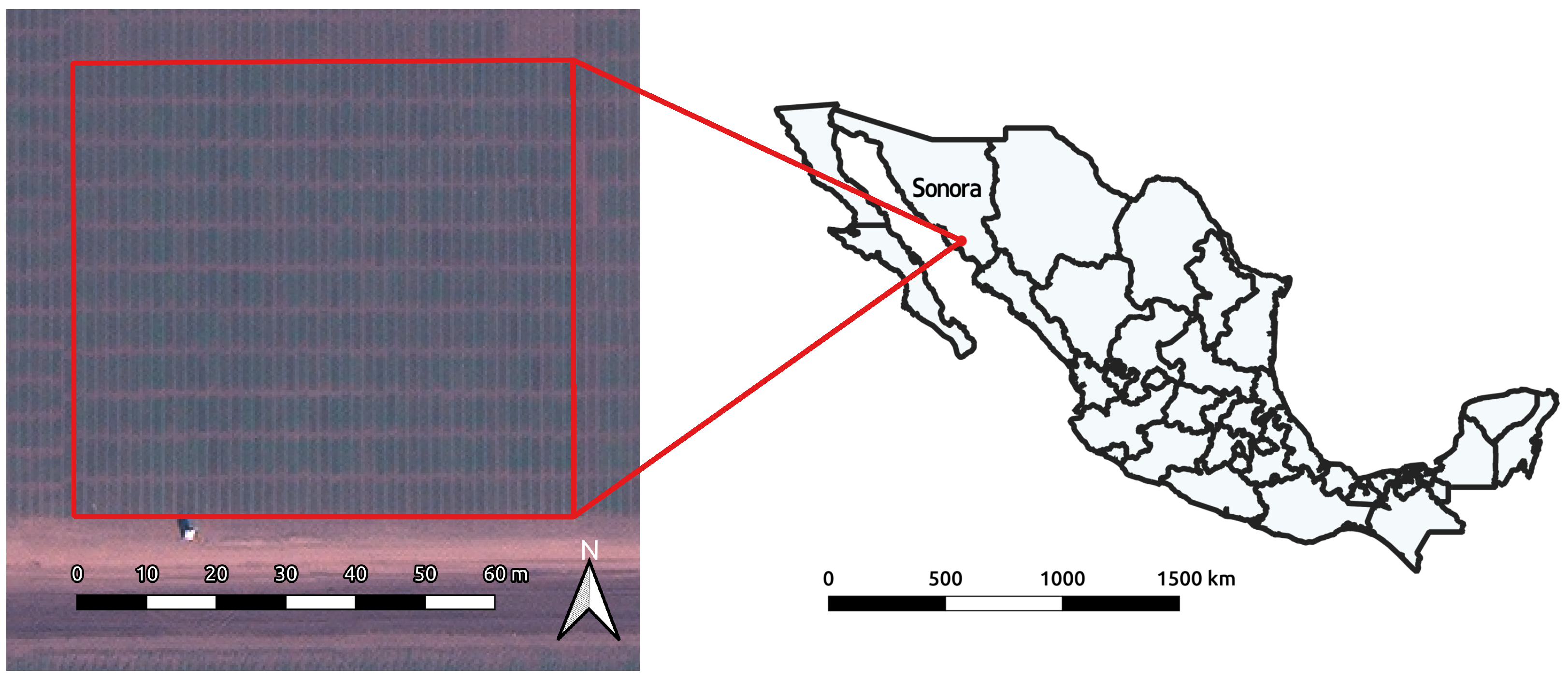
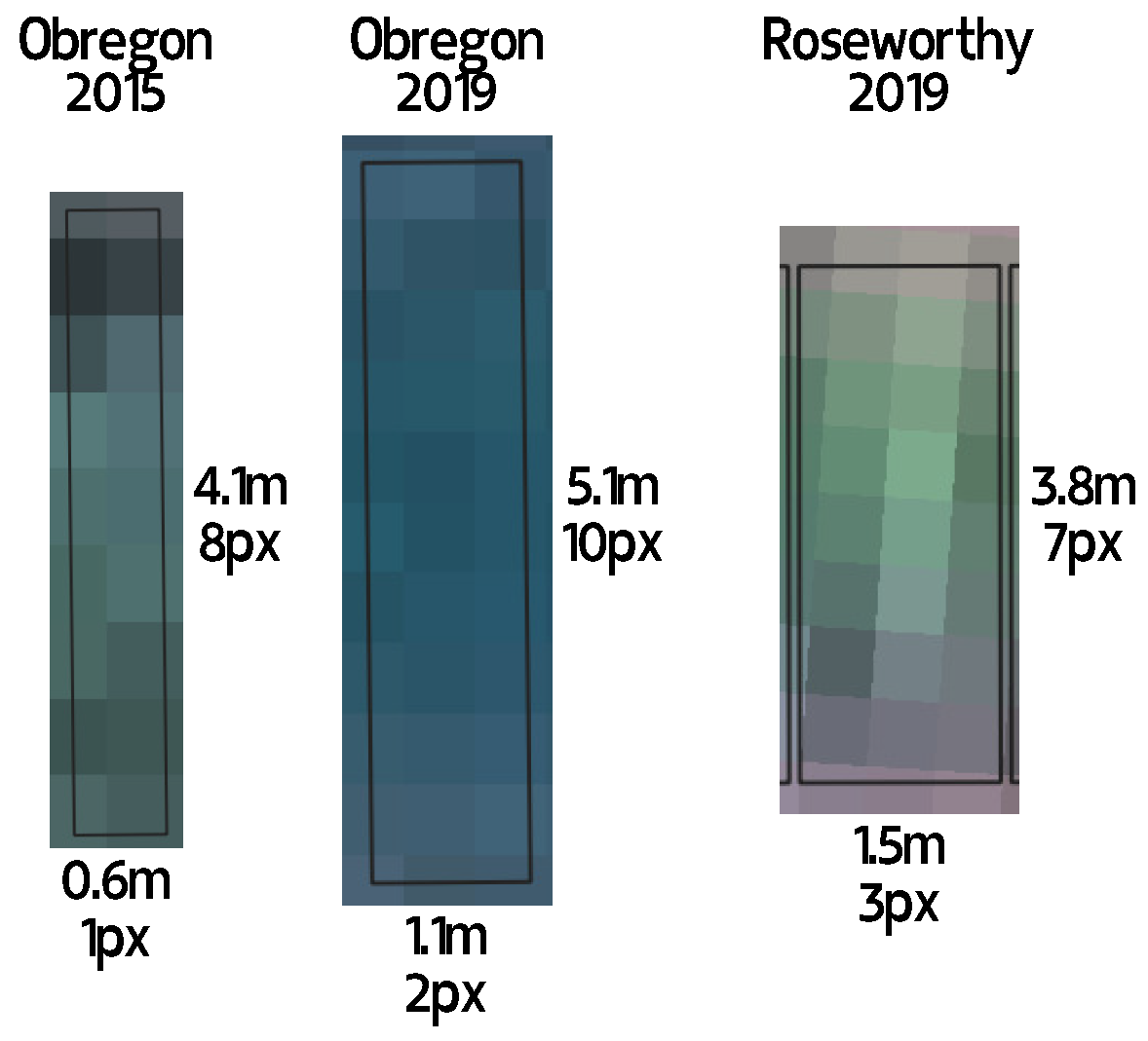
Our image data consisted of 14 images from two separate trial sites on different continents. The images were from the KOMPSAT-3a (K3a), GeoEye-1 (GE1), WorldView-2 (WV2), and WorldView-3 (WV3) satellites. These satellites have panchromatic resolutions of 55 cm, 41 cm, 46 cm, and 31 cm, respectively. The WV2 and WV3 satellites have 8 spectral bands, but the GE1 and K3a satellites only have 4 (red, green, blue, and near infrared). Thus, we only used these four bands from all of our satellite images.

2.1.2. Roseworthy

The Roseworthy site (34.5°S, 138.7°E) is located near the South Australian town of Roseworthy (see Figure 1). This site is in a representative grain-growing region of Australia’s southern wheat belt, representing a long-term stable environment where breeding trials have been carried out for over 100 years. In 2019, Australian Grain Technologies (AGT) performed standard crop trials with 1464 canola lines at their Roseworthy site. Each plot covered approximately 5.75 m 2 , and the total area was 14 , 700 m 2 . During this trial, they measured several traits at multiple time points during the season: canopy cover, greenness, flowering, and height.
Canopy cover is the percentage of soil surface covered by plant foliage and is a measurement of establishment and early vigour. Greenness is a broad estimation of general vigour. Flowering is the percentage of blooming buds on each stem. Seven UAV mosaics were obtained from a DJI Phantom 4 Pro throughout the season. Canopy cover, greenness, and flowering were measured via image analysis by Hiphen; a business specialising in agricultural image analysis. Height is a coarse measurement of overall plant growth and was measured in the field using a ruler.
To assemble our Roseworthy dataset, AGT generously provided their 2019 crop trial measurements, and we purchased five very high-resolution satellite images taken during the same time period. These consisted of one GE1 image, two WV2 images, and two WV3 images. Altogether, we had 1464 plots × 5 images = 7320 data points for each canola trait. The plots’ spatial boundaries were not initially recorded by AGT, but the individual plots were visibly distinct in the satellite images. So, we drew a uniform grid of all plot boundaries onto the satellite images to match the pixels to the recorded ground measurements.

2.1.3. Obregón

The Obregón site (27.4°N, 109.9°W) is located in Sonora, Mexico near the town of Ciudad Obregón (see Figure 2). This site is in the Northwestern grain growing region of Mexico, chosen by CIMMYT as a key region for global wheat breeding. The data for the Obregón site were split into two trials covering different areas, with different plot sizes. In 2015, the trial area was 6180 m 2 , and each plot was 2.48 m 2 . In 2019, the trial area was 4610 m 2 and each plot was 5.72 m 2 .
For over 50 years, the International Maize and Wheat Improvement Center (CIMMYT) has performed crop trials on wheat, collecting various data from hundreds of thousands of plots. CIMMYT generously provided their measurements during their 2015–2016, 2016–2017 and 2019–2020 crop trials for our research. For each growing season during this period, they measured above-ground biomass and ground NDVI multiple times. In-season biomass tracks crop growth rate and consequently determines a plot’s radiation use efficiency (RUE) and photosynthetic efficiency. The in-season above-ground biomass was measured through cutting, drying, and weighing a 50 cm quadrat sample of plants. Ground NDVI is a simple measure of general plant growth and is strongly associated with canopy size, greenness, and pre-anthesis biomass. It was measured with a Greenseeker NDVI portable sensor. More details can be found in CIMMYT’s published data collection protocols [59].
NDVI, being a vegetation index, can be directly calculated from a satellite image, but this is not the same NDVI that is measured at ground level using hand-held devices. These measurements are taken at different times, using different bandwidth sensors, covering different physical areas, and under different lighting/atmospheric effects. Predicting the ground NDVI from the satellite colour bands is useful as an estimate of consistency between ground and satellite sources. Assuming a reliable mapping can be found, NDVI predictions can be fed into existing models that relate ground NDVI to other ground properties, such as canopy cover or greenness.
We purchased nineteen very high-resolution satellite images taken during CIMMYT’s 2015–2016, 2016–2017, and 2019–2020 crop trials. Four of these images were from the Deimos-2 and KOMPSAT-2 satellites. Since these have a panchromatic resolution of 1 m, the images did not have a high enough resolution to distinguish between plots in the trials. Additionally, we were unable to adequately align the images for the 2016–2017 crop trial. This left us with three images for the 2015–2016 crop trial (two WV2 and one GE1) and six images for the 2019–2020 crop trial (one K3a, two GE1, two WV2, and one WV3). In the 2015 trial, there were 1200 smaller plots—0.6 m × 4.1 m—and in the 2019 trial there were 450 larger plots—1.1 m × 5.1 m. Unfortunately, many plots/measurements were excluded due to some plots being measured just once, poor alignment between image and measurement, and plots not containing whole distinct pixels. For example, NDVI was not measured in 2015, and only 2/3 of the plots had multiple biomass measurements. Altogether, we included 1200 data points for NDVI and 2385 data points for biomass.
The plot boundaries were smaller at Obregón than at Roseworthy, and the plots were closer together. This made image alignment more difficult, as the plot boundaries were not visible within our satellite images. We addressed this by utilising UAV footage, which was taken during the crop trials. Crop boundaries were drawn to align with the UAV imagery, and the satellite images were then spatially aligned to match the UAV footage using various landmarks. This ultimately allowed us to assign satellite image pixels to specific plots.

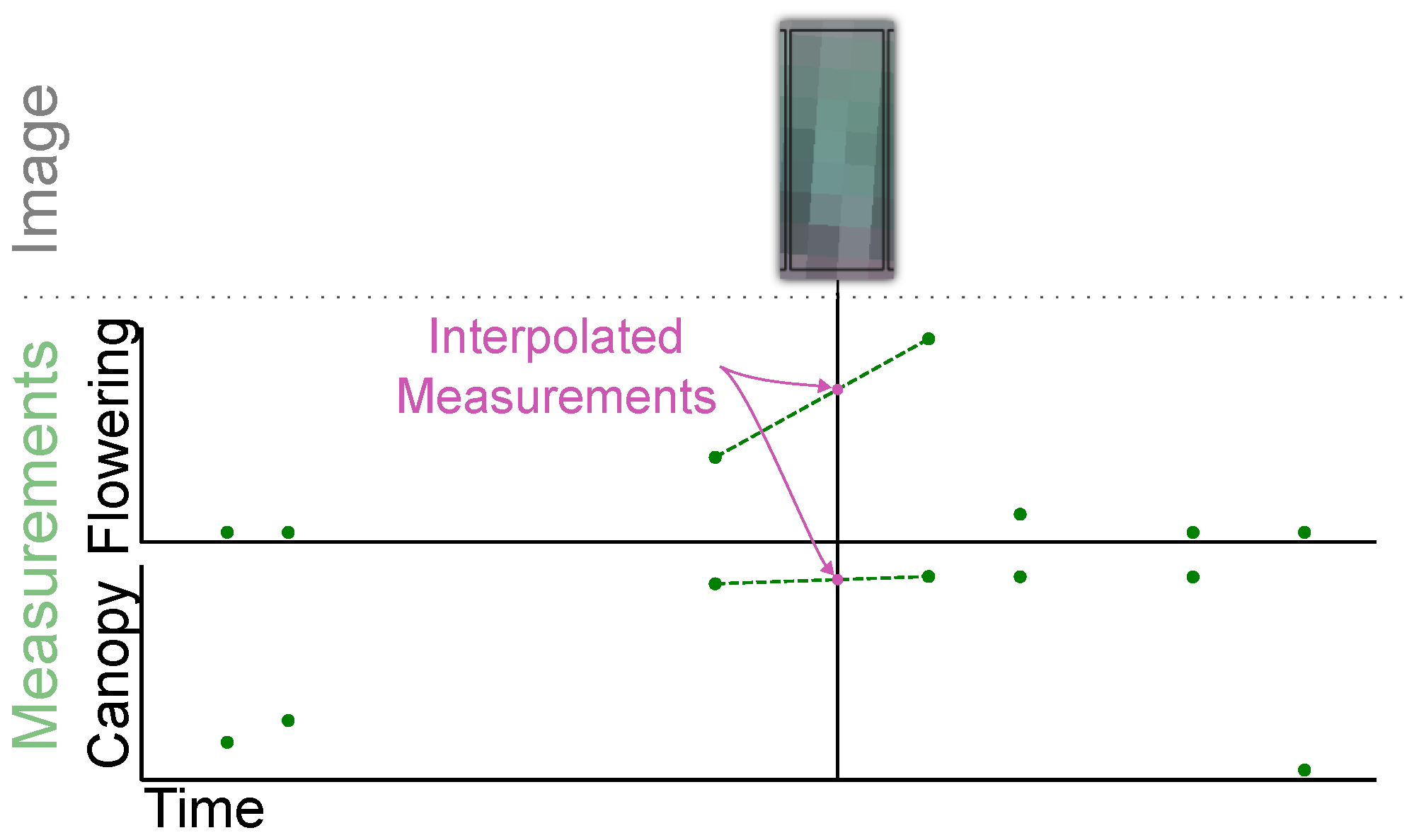
2.1.4. Ground Data Interpolation

Since the satellite images were purchased retroactively, they did not precisely match the times that the ground measurements were taken. To account for this, labels for each plot were determined by linearly interpolating between the nearest two ground measurements. We are cognisant of the fact that linear interpolation introduces error, and this error is directly related to the infrequency and non-linearity of the measured values. Figure 3 shows the most extreme case for interpolation of Roseworthy Image 3, which was eight days away from the nearest ground measurement. The median time to the nearest ground measurement for the interpolated values was 4 days for Roseworthy, 3.2 days for Obregón (Biomass), and 2.5 days for Obregón (NDVI). Plants undergoing senescence generally do not vary linearly. Consequently, we did not extrapolate after the last measurement for any trait, even though none of the images showed large amounts of senescence. We only extrapolated earlier in the season, where we saw reliable trends towards zero in our data. This included all traits except NDVI.

2.1.5. Image Preprocessing

The images were converted to reflectances using published information about the sensors for GeoEye-1, WorldView-2, WorldView-3 [60], and KOMPSAT-3a [61] along with the exoatmospheric solar irradiance measurements by Thuiller et al. [62]. The images were then pansharpened using the Weighted Brovey algorithm, as implemented in the GDAL library [63]. All images were taken during very clear days, so it was not necessary to perform any additional atmospheric correction.
The initial spatial alignment from the image providers had error in the order of metres, which was not precise enough for this work. The plots on the ground are less than 1.5 m in either dimension (see Figure 4), so a misalignment of more than one pixel would completely misalign the ground measurements with the pixels that the plots occupy. We annotated between 4 and 40 ground control points on each image to align them using a combination of Quantum GIS (QGIS) software and external scripts. In general, precisely aligning images (georeferencing) involves resampling the image to warp the images and match the coordinate systems. Resampling is equivalent to a small amount of blurring, which we wanted to avoid in order to preserve image integrity. Therefore, the images were aligned by modifying only the geotransform, to avoid the blurring effect, and only precisely aligned within the field of interest.

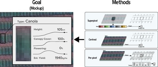
2.2. Methods for Per-Plot Prediction

The goal of this work was to create a model capable of predicting phenotypic traits for each plot in an image. The algorithm, denoted f θ , must take an image X R H × W × C and make a prediction f θ ( X ) = Y ^ R N × P for each plot in that image, ideally which matches the ground measurements Y R N × P . Where H is the image height, W is the image width, C = 4 is the number of colour bands (red, green, blue and near infrared), N is the number of visible plots, and P is the number of properties being predicted. All models were trained with the supervised learning objective of minimising mean squared error (MSE).
L ( Y , Y ^ ) = MSE ( Y , Y ^ ) = ( Y i Y ^ i ) 2
We describe three different methods used to perform these predictions: superpixel, centred, and per-pixel (see Figure 5). The superpixel method (also known as object-based or OBIA) is an existing method [51,52], which we present as a baseline. This method uses aggregated statistics of the pixels contained within the plot boundaries and lacks any contextual information. There are a number of reasons why the aggregated statistics of only the pixels within the plot boundaries may not provide enough information to make accurate predictions. For example, the whole image might have a slight blue tinge due to atmospheric haze. Without the contextual information that everything appears slightly more blue than usual, the superpixel method cannot detect and automatically adjust its prediction in response. Additionally, the plot boundaries are unlikely to precisely align with the pixels in the crop. Sometimes they will include some of the ground or a neighbouring plot. The superpixel method has no way to distinguish between pixels that are relevant and those that are not. In contrast, a CNN is able to see the intra-plot spatial structure and can learn which pixels are important. So, here, we propose two novel methods for making per plot predictions: centred and per-pixel. These methods use contextual information and thus are empowered to handle the aforementioned problems automatically.

2.2.1. Superpixel

The superpixel method uses the known plot boundaries to extract a subset of pixels from X for each separate plot and independently aggregates the colour information to form a fixed-length feature vector for each plot V R N × D . This condenses an arbitrary number of pixels into a fixed-length vector of size D. Fixed-length input vectors can be used by many kinds of machine learning models, including random forest (RF) [64], extreme gradient boosting (XGB) [65], support vector machine (SVM) [66], and multilayer perceptron (MLP/ANN) [67].
We used RF and MLP models to represent the superpixel method. These are two very common algorithms used for remote sensing tasks, and they performed better on average than XGB and SVM in our preliminary testing. We aggregated statistics across all pixels that intersected each plot’s boundary, to create a vector of size D = 15 for each plot. These statistics consisted of the minimum, mean, and maximum of each colour band, as well as a derived NDVI channel.

2.2.2. Centred

The centred method directly uses pixel information from a small image crop centred on a plot X ^ R 32 × 32 × C to predict for a single plot at a time y ^ R P . This specifically provides contextual information, so that the model has a chance to learn to adjust its predictions based on that context. Since the prediction refers only to the centre of the image, the centred method also does not depend on knowledge of the plot boundary, making it more flexible than the superpixel method.
A centred method was constructed for use with a straight-forward CNN architecture and applied to per-plot predictions. The centred method uses a whole image crop to regress to continuous, real-valued numbers. Classification models could be adapted for regression, which allowed us to use existing well-known image classification architectures in the centred method. We replaced both the first and last layers of these architectures. Replacing the last layer is standard for transfer learning, because the original models were designed for a different task. Unlike typical transfer learning, replacing the first layer was also necessary here because pretrained CNNs use only RGB colour bands, but our data also have the NIR colour band. To handle this, a new first layer was initialised, which used 4 colour bands, and only the pretrained weights for the RGB bands were copied. The remaining NIR band weights were randomly initialised, so we also fine-tuned all weights throughout the model.
The best known classification architectures were initially created for the ImageNet dataset [68], using an input crop size of 224. However, because the plots being imaged were barely more than 3 pixels in each dimension, such an input size would contain much more information than is necessary. So here, we used a crop size of 32 × 32, which represents a side length somewhere between 10 and 16 m, depending on image resolution. This value was chosen to align with the well-known CIFAR10 dataset. Due to the popularity of both datasets, architectures designed for ImageNet have been minimally adapted to the input of 32 × 32 used in CIFAR10 [69]. Thus, we compared VGG-A, ResNet18, ResNet50, and Densenet161 models that were modified to work on CIFAR10, and used weights pretrained on CIFAR10.

2.2.3. Per-Pixel

The centred method is somewhat inefficient, because to predict for just the plot in the centre we must feed it an image crop which contains many other plots. In order to predict for a whole image, this requires running a sliding window across the whole field area, frequently repeating calculations on contextual pixels. The per-pixel method is designed to generalise the centred method to predict for all pixels within a crop X ^ R 128 × 128 × 4 in a single pass of the network.
By predicting per-pixel, the number of outputs scales with the number of inputs, which theoretically makes it more efficient than the centred method. Thus, we used a crop size of 128 × 128 for the per-pixel methods, to give the model even more context.
Our per-pixel model does not make per-plot predictions directly, so we introduced fixed functions to translate between per-plot and per-pixel values, and vice versa. A per-pixel-to-per-plot fixed function aggregates model predictions identically to the way the superpixel method aggregates input pixels. A per-plot-to-per-pixel fixed function spatially duplicates the per-plot labels to render a per-pixel prediction map. These fixed functions introduce two new hyperparameters. The first hyperparameter is an overlap threshold, which determines when a pixel is considered part of a plot. We trialled several values during preliminary testing and found that an overlap threshold of 75% was most effective. Below 75%, the results were dramatically worse, but there was little difference between 75% and 100%. The second hyperparamenter is the aggregation function used to aggregate per-pixel predictions within a plot. We used the 75th percentile of the included predicted pixel values to make a per-plot prediction, because of the large proportion of mixed pixels, which we assumed would be given a lower value.
The per-pixel method is a form of dense prediction, which mirrors the common computer vision task of semantic segmentation. Consequently, we were able to experiment with well-known segmentation architectures as the backbones of our per-pixel CNN models. In this work, we compared the UNet++ [31] and DeepLabv3 [70] models, as they are two popular generic segmentation architectures. We did not use transfer learning for these models because it did not improve the results during preliminary testing.

2.3. Training Details

Each of the 5 images for Roseworthy and 9 images for Obregón showed different stages of growth, so they could not meaningfully be split into train/test by image. Instead, we split by groups of rows in the image (see Figure 6). All results shown here were cross-validated across 4 (Roseworthy) or 6 (Obregón) folds. All reported results are for the full cross-validation, but all hyperparameters were tuned on the first fold only. Additionally, the hyperparameters were determined by training models that predicted all properties at Roseworthy at once. However, the results were obtained by training a separate model per trait to optimise individual performance. More training details can be found in the Supplementary Materials.

3. Results

We trained superpixel (RF and MLP), centred (VGG-A, ResNet18, ResNet50, and DenseNet161), and per-pixel (UNet++ and DeepLabv3) models on both Roseworthy (Table 1) and Obregón (Table 2) data. The models were cross-validated across the folds described in Figure 6 to obtain error bars. A separate model was trained independently on each trait, and the hyperparameters did not change across the traits or folds. Strikingly, there was only a small difference in overall predictive ability between models, despite the large difference in computation required.
We posit that the performance of all models was generally quite high because there was a bias in our data that promoted predicting the average trait value for each image. This bias existed because there was a strong relationship between trait value and days after sowing (DAS). Each image presented the model with a unique DAS, and there were few images, which led to a strong relationship between trait value and image in our training data (see Figure 7).Using DAS to inform predictions is not a problem in general, but there is a hypothetical degenerate solution where the model can obtain a relatively high R 2 without ever looking at the plots individually. This is because a model could theoretically learn to identify each image, determine the average trait value for that particular DAS, and then use that average value as its prediction. Such a model is undesirable, as it would be unable to distinguish between plots or generalise effectively to new images. We calculated the performance of such a degenerate solution and include it as a point of reference for the high R 2 values in the overall results (Table 1 and Table 2).
Among the Roseworthy traits, the hypothetical degenerate solution was most prominent for canopy cover. In Table 1 and Figure 7, we show that canopy cover was almost entirely predictable using DAS. There was very little variation for canopy cover within each image, and thus little room for improvement with machine learning on this trait. In contrast, flowering had more variation within each image, and thus more opportunity for machine learning. Indeed, all machine learning models substantially outperformed the degenerate hypothetical solution for flowering. Thus, while the R 2 values were inflated by the image-average bias (see Figure 8), the models learned a more substantial relationship than just the image-average bias.
The Roseworthy results show that a consistent model performed best within each method: MLP was the best superpixel model, ResNet18 was the best centred model, and UNet++ was the best per-pixel model. The superpixel models performed surprisingly well overall, despite being simpler and lacking context from surrounding pixels. The superpixel MLP even outperformed the per-pixel DeepLabv3 model. However, the centred ResNet18 and UNet++ performed equally or better than the superpixel MLP on all Roseworthy traits. This shows that the contextual pixels provided some value. The centred ResNet18 model performed the best overall; however, the per-pixel UNet++ model was equivalent to the ResNet18 model on three out of the four properties, with a large error bar for flowering, so it is difficult to differentiate the two.
For Obregón, several models were not able to improve on the performance of the hypothetical degenerate solution (Table 2). This is likely due to the relatively small amount of training data at this site and the unknown amount of spatial alignment error between images creating confusing labels. Similarly to the Roseworthy site, the centred and per-pixel methods slightly outperformed the superpixel methods at the Obregón site. However, the Obregón results were less reliable. The variance between folds for the Obregón site was substantially larger than for the Roseworthy site, and there was no consistent best model across traits within each method. Since the Obregón results were unreliable, they provide only weak evidence that ResNet18 was the best model.

3.1. High-Variance Per-Image Evaluation

We noticed a strong image-average bias during early experimentation. This bias was concerning, because a key end-use for predicting canopy phenotype traits is to differentiate between plots within the same image. This motivated us to more clearly evaluate how effectively our machine learning models could differentiate between plots. Figure 8 shows the predictions of a Roseworthy height model. It shows that that two of the images have trait values mostly around 0, which the model correctly predicted as very low values. However, the relative trait values in the images with a higher variance were much less accurate. Thus, we evaluated our models only on high-variance images to directly measure each model’s ability to differentiate within an image (see Table 3). For the low-variance images, the trait values were very similar, showing plots at similar stages of growth and the model would have been completely correct to use the average trait value. For the high-variance images, the trait values were quite different, showing plots at different stages of growth, and the model would have been incorrect to use the average trait value. We defined high-variance images as those which had at least 5% of the total variation visible within the image. To remove any benefit from predicting the per-image average, we measured R 2 within each image independently.
When we evaluated only using high-variance images, we observed a substantially lower R 2 than for the overall results. These results better reflected the model performance within a single image. But they also represented a substantially more difficult challenge, because the models received no benefit for being able to correctly identify image and implicitly used the DAS to inform predictions. Instead, the models were solely evaluated on their ability to distinguish between values within an image. Whereas the overall results describe an absolute measurement of model performance, these high-variance results describe how clearly the model could identify plots that, for example, began flowering earlier than others or reached certain heights before others. Despite being numerically lower, these results are consistent with the overall results, showing a clear improvement of the centred ResNet18 and per-Pixel UNet++ over the superpixel MLP. This reinforces that, when models are not able to use the per-image average, the ability of CNN models to consider contextual pixels still improves prediction accuracy.
Note that there were no images with sufficient variance in NDVI, and several models learned to predict a single biomass value for each image, which gives further evidence that the results from Obregón are unreliable.

3.2. High-Variance Image Training

If a major end-use of the models is to be able to differentiate between plots within an image, then one might wonder if there is some benefit to only training the models on high-variance images. This might be beneficial, because it would force the model to ignore the identification of the image and emphasise learning to identify features useful in general. However, this might be a disadvantage, because restricting the dataset naturally means showing fewer independent examples.
To test this, we selected the two best performing models (ResNet18 and UNet++) and compared training them on the overall dataset vs. training them using only the high-variance images. To make it a fair comparison, we conducted a new hyperparameter search for each of these models on the restricted dataset. We found that training only on the high-variance images generally decreased performance on those images for both the ResNet18 and the UNet++ model (see Table 4). This implies that the model was more disadvantaged by restricting the dataset than it was advantaged by using a dataset that was more aligned with differentiating between plots.

4. Discussion

While the different methods are only presented as competing on R 2 , their different properties mean they have different costs, benefits, and opportunities. Superpixel methods are much faster than deep learning-based centred and per-pixel methods. The superpixel and per-pixel methods require that precise plot boundaries are known, whereas the centred method only requires the centre of the plot, making the centred method the most flexible. Additionally, most existing works at a similar scale pose per-pixel problems [22,24]. Thus, our per-pixel models are most appropriate for transfer learning between our task and other remote sensing tasks.
The lower accuracy we observed in the per-image results for high-variance images was not completely unexpected. On top of the small dataset, there was some unknown amount of error in creating the ground labels used for training. At the ground level, there was error with the instruments used to measure the traits. Then, there was some error in calculating reflectances across different satellites and days [71]. While our image capture and ground measurement dates aligned reasonably well, the necessary linear interpolation would still have introduced noteworthy uncertainty to any labels. And finally, there was error in how well aligned the images could be with the plot boundary annotations. These factors combined to make the labels somewhat error-prone in the applied settings.
The scale of data is important here. In this work, we show that, using just a handful of images in one field, we can learn a small–moderate correlation between satellite image data and plant traits. To progress further in this direction, it is clear that larger datasets are required. Measuring the 1464 plots at Roseworthy multiple times per season represents a substantial effort for agronomists, but data from a single site are unlikely to generalise well to other sites [72]. A future model that could operate across sites and years would need both training data showing such variation and testing data to show that it is effective. Models trained on larger datasets are also less prone to overfitting and more robust to errors in measurement. As such, more samples are needed, but this promises substantial performance improvements.
Using only a handful of images limits the models’ ability to generalise, as only a limited range of plant growth is represented. However, it is not as dire as it first appears, as each plot develops at a slightly different rate, and thus their phenotypic traits vary from plot to plot, even within the same image. This is precisely why high-variance images exist. So, although there were only five images, there are thousands of slightly different development stages represented. Unfortunately, the early growth stages were especially poorly represented in our data. For future work, we could represent more varied stages of plant growth within a single image by staggering the planting of the plots or by using breeds with very different flowering times.
Many of the sources of noise in image data could be mitigated by pro-actively collecting images from the same satellite during future trials. For example, the misalignment between image times and key biological dates could be reduced further by coordinating ground measurements with image captures. Additionally, by tasking a satellite, we could collect data that better represents the whole growing season. Here, we show a promising minimum performance that will only improve as satellite images become cheaper, more frequent, and more accessible.

Limit of Resolvability

In related UAV research, it is common to discard mixed pixels at the edges of the plot boundary [5,58]. However, when using satellite imagery for per-plot predictions, there are very few pixels to work with, so each pixel is valuable, and discarding pixels on the border of the plot boundaries needs to be carefully considered. For smaller plot boundaries, and for coarser resolution images, this is a greater problem. Eventually, if the plot boundaries are too small compared to the resolution of the image, it becomes impossible to reliably select the pixels that primarily contain the plants in question (see Figure 4). We call this the limit of resolvability, and in this work we showed results all the way up to this limit. In this work, we were forced to use some mixed pixels, otherwise many more plots would have had no pixel data. However, even this substantial challenge did not prevent us from making a model that could predict phenotypic traits.
The Roseworthy data used plots sized 1.5 m × 3.8 m, which were approximately 3 pixels across for our coarsest image (50cm resolution) and showed robust results across all folds, for all models. The Obregón data used plots sized 0.6 m × 4.1 m for the 2015 data, and 1.1 m × 4.8 m plots for the 2019 data. The NDVI was only recorded for the 2019 trial, so the biomass models were the only ones to use the smallest plots at only one pixel across. The biomass results were unreliable, likely due to a combination of the relatively small plots and the inherent difficulty in predicting biomass from satellite imagery. The NDVI results showed a high overall R 2 ; however, all of the images had a low variance in NDVI, so we could not evaluate them per-image. Qualitatively, however, all of the models preferred predicting the mean value per image for NDVI more than for any trait at Roseworthy, and for some models, the performance variance across folds was also very high (see Table 2).
This work, then, describes results at three levels increasingly close to the limit of resolvability (Roseworthy canola traits, CIMMYT wheat NDVI, and CIMMYT wheat biomass), and shows that the results became increasingly less reliable towards this limit. It should be noted that there are more factors than just resolution that explain these unreliable results, but clearly the resolution and plot size at Roseworthy was sufficient for generating robust prediction models. Thus, we make a suggestion for any future work: to stay clear of the limit of resolvability, the plots in the image must contain at least three pixels in each dimension.

5. Conclusions

We worked at the limit of resolvability and showed that promising plot-level predictions can be made with only a handful of satellite images. We proposed two novel methods for spatial CNNs to predict phenotypic traits at a per-plot level and compared them against more traditional superpixel methods. We showed that even with this small dataset, spatial CNNs can improve predictions for phenotypic traits from satellite images. Although the improvement in the overall metrics between these methods was limited, this was largely a consequence of the average for each image being a very strong baseline. Our analysis found that the CNN methods performed better than the superpixel methods, both for overall metrics and when using a restricted dataset of images with high label variance. We posit that this was because contextual pixels and intra-plot spatial information hold predictive power that is inaccessible to superpixel models. In particular, the centred ResNet18 and per-pixel UNet++ models performed best. Out of these, due to its simplicity, we recommend the centred ResNet18 model for high-throughput quantitative phenotyping. More generally, we suggest that these results point to the exciting future utility of high-resolution satellites and machine learning for constructing prediction models and informing the breeding of vital crops.

Supplementary Materials

The following supporting information can be downloaded at: https://www.mdpi.com/article/10.3390/rs16020282/s1, Table S1: Model hyperparameters.

Author Contributions

Conceptualisation, S.J.N. and R.T.F.; data curation, T.C., F.P. and M.R.; formal analysis, B.V.; investigation, B.V.; methodology, B.V., A.N. and Z.H.; software, B.V.; supervision, A.N., Z.H. and R.T.F.; writing—original draft preparation, B.V.; writing—review and editing, B.V., A.N., S.J.N., T.C., F.P., M.R., R.T.F. and Z.H. All authors have read and agreed to the published version of the manuscript.

Funding

This research received no external funding.

Data Availability Statement

The data used in this work have not been made publicly available. The purchased images were only licensed for internal use, not for sharing to the public. The ground measurements used are private data of AGT and CIMMYT, respectively.

Acknowledgments

This work was supported by the SmartSat CRC, whose activities are funded by the Australian Government’s CRC Program. The images were purchased with funds provided by an internal grant from the Centre for Entrepeneurial Agritechnology at ANU. We also wish to thank our industry partners Australian Grain Technologies (AGT) and International Maize and Wheat Improvement Centre (CIMMYT), who shared ground-truth data and without which this work would not have been possible.

Conflicts of Interest

The authors declare no conflict of interest.

References

  1. Tilman, D.; Balzer, C.; Hill, J.; Befort, B.L. Global Food Demand and the Sustainable Intensification of Agriculture. Proc. Natl. Acad. Sci. USA 2011, 108, 20260–20264. [Google Scholar] [CrossRef] [PubMed]
  2. Garnett, T.; Appleby, M.C.; Balmford, A.; Bateman, I.J.; Benton, T.G.; Bloomer, P.; Burlingame, B.; Dawkins, M.; Dolan, L.; Fraser, D.; et al. Sustainable Intensification in Agriculture: Premises and Policies. Science 2013, 341, 33–34. [Google Scholar] [CrossRef]
  3. Campos, H.; Cooper, M.; Habben, J.E.; Edmeades, G.O.; Schussler, J.R. Improving Drought Tolerance in Maize: A View from Industry. Field Crop. Res. 2004, 90, 19–34. [Google Scholar] [CrossRef]
  4. White, J.W.; Andrade-Sanchez, P.; Gore, M.A.; Bronson, K.F.; Coffelt, T.A.; Conley, M.M.; Feldmann, K.A.; French, A.N.; Heun, J.T.; Hunsaker, D.J.; et al. Field-Based Phenomics for Plant Genetics Research. Field Crop. Res. 2012, 133, 101–112. [Google Scholar] [CrossRef]
  5. Chapman, S.C.; Merz, T.; Chan, A.; Jackway, P.; Hrabar, S.; Dreccer, M.F.; Holland, E.; Zheng, B.; Ling, T.J.; Jimenez-Berni, J. Pheno-Copter: A Low-Altitude, Autonomous Remote-Sensing Robotic Helicopter for High-Throughput Field-Based Phenotyping. Agronomy 2014, 4, 279–301. [Google Scholar] [CrossRef]
  6. Sankaran, S.; Marzougui, A.; Hurst, J.P.; Zhang, C.; Schnable, J.C.; Shi, Y. Can High-Resolution Satellite Multispectral Imagery Be Used to Phenotype Canopy Traits and Yield Potential in Field Conditions? Trans. ASABE 2021, 64, 879–891. [Google Scholar] [CrossRef]
  7. Hedden, P. The Genes of the Green Revolution. Trends Genet. 2003, 19, 5–9. [Google Scholar] [CrossRef]
  8. Awulachew, M.T. Understanding Basics of Wheat Grain and Flour Quality. J. Health Environ. Res. 2020, 6, 10. [Google Scholar] [CrossRef]
  9. Fischer, R.; Byerlee, D.; Edmeades, G. Crop Yields and Global Food Security: Will Yield Increase Continue to Feed the World? Number 158 in ACIAR Monograph; Australian Centre for International Agricultural Research: Canberra, Australia, 2014. [Google Scholar]
  10. Furbank, R.T.; Sirault, X.R.; Stone, E.; Zeigler, R. Plant Phenome to Genome: A Big Data Challenge. In Sustaining Global Food Security: The Nexus of Science and Policy; CSIRO Publishing: Clayton, Australia, 2019; p. 203. [Google Scholar]
  11. MacDonald, R.B.; Hall, F.G. Global Crop Forecasting. Science 1980, 208, 670–679. [Google Scholar] [CrossRef]
  12. Zhou, L.; Tucker, C.J.; Kaufmann, R.K.; Slayback, D.; Shabanov, N.V.; Myneni, R.B. Variations in Northern Vegetation Activity Inferred from Satellite Data of Vegetation Index during 1981 to 1999. J. Geophys. Res. Atmos. 2001, 106, 20069–20083. [Google Scholar] [CrossRef]
  13. White, M.A.; De BEURS, K.M.; Didan, K.; Inouye, D.W.; Richardson, A.D.; Jensen, O.P.; O’keefe, J.; Zhang, G.; Nemani, R.R.; Van Leeuwen, W.J.D.; et al. Intercomparison, Interpretation, and Assessment of Spring Phenology in North America Estimated from Remote Sensing for 1982–2006. Glob. Chang. Biol. 2009, 15, 2335–2359. [Google Scholar] [CrossRef]
  14. Kang, Y.; Ozdogan, M.; Zhu, X.; Ye, Z.; Hain, C.; Anderson, M. Comparative Assessment of Environmental Variables and Machine Learning Algorithms for Maize Yield Prediction in the US Midwest. Environ. Res. Lett. 2020, 15, 64005. [Google Scholar] [CrossRef]
  15. Potopova, V.; Trnka, M.; Hamouz, P.; Soukup, J.; Castravet, T. Statistical Modelling of Drought-Related Yield Losses Using Soil Moisture-Vegetation Remote Sensing and Multiscalar Indices in the South-Eastern Europe. Agric. Water Manag. 2020, 236, 106168. [Google Scholar] [CrossRef]
  16. Eroglu, O.; Kurum, M.; Boyd, D.; Gurbuz, A.C. High Spatio-Temporal Resolution CYGNSS Soil Moisture Estimates Using Artificial Neural Networks. Remote Sens. 2019, 11, 2272. [Google Scholar] [CrossRef]
  17. Senanayake, I.P.; Yeo, I.Y.; Walker, J.P.; Willgoose, G.R. Estimating Catchment Scale Soil Moisture at a High Spatial Resolution: Integrating Remote Sensing and Machine Learning. Sci. Total Environ. 2021, 776. [Google Scholar] [CrossRef]
  18. Sakamoto, T.; Gitelson, A.A.; Arkebauer, T.J. MODIS-based Corn Grain Yield Estimation Model Incorporating Crop Phenology Information. Remote Sens. Environ. 2013, 131, 215–231. [Google Scholar] [CrossRef]
  19. Waldner, F.; Diakogiannis, F.I.; Batchelor, K.; Ciccotosto-Camp, M.; Cooper-Williams, E.; Herrmann, C.; Mata, G.; Toovey, A. Detect, Consolidate, Delineate: Scalable Mapping of Field Boundaries Using Satellite Images. Remote Sens. 2021, 13, 2197. [Google Scholar] [CrossRef]
  20. Rahman, M.M.; Robson, A.; Bristow, M. Exploring the Potential of High Resolution WorldView-3 Imagery for Estimating Yield of Mango. Remote Sens. 2018, 10, 1866. [Google Scholar] [CrossRef]
  21. Ferreira, M.P.; Lotte, R.G.; D’Elia, V.F.; Stamatopoulos, C.; Kim, D.H.; Benjamin, A.R. Accurate Mapping of Brazil Nut Trees (Bertholletia Excelsa) in Amazonian Forests Using WorldView-3 Satellite Images and Convolutional Neural Networks. Ecol. Inform. 2021, 63, 101302. [Google Scholar] [CrossRef]
  22. Ahlswede, S.; Asam, S.; Roeder, A. Hedgerow Object Detection in Very High-Resolution Satellite Images Using Convolutional Neural Networks. J. Remote Sens. 2021, 15. [Google Scholar] [CrossRef]
  23. Saralioglu, E.; Gungor, O. Semantic Segmentation of Land Cover from High Resolution Multispectral Satellite Images by Spectral-Spatial Convolutional Neural Network. Geocarto Int. 2022, 37, 657–677. [Google Scholar] [CrossRef]
  24. Mei, W.; Wang, H.; Fouhey, D.; Zhou, W.; Hinks, I.; Gray, J.M.; Van Berkel, D.; Jain, M. Using Deep Learning and Very-High-Resolution Imagery to Map Smallholder Field Boundaries. Remote Sens. 2022, 14, 3046. [Google Scholar] [CrossRef]
  25. LeCun, Y.; Boser, B.; Denker, J.S.; Henderson, D.; Howard, R.E.; Hubbard, W.; Jackel, L.D. Backpropagation Applied to Handwritten Zip Code Recognition. Neural Comput. 1989, 1, 541–551. [Google Scholar] [CrossRef]
  26. Krizhevsky, A.; Sutskever, I.; Hinton, G.E. ImageNet Classification with Deep Convolutional Neural Networks. In Proceedings of the Advances in Neural Information Processing Systems; Curran Associates, Inc.: Red Hook, NY, USA, 2012; Volume 25, pp. 1106–1114. [Google Scholar]
  27. He, K.; Zhang, X.; Ren, S.; Sun, J. Deep Residual Learning for Image Recognition. arXiv 2015, arXiv:cs/1512.03385. [Google Scholar] [CrossRef]
  28. Sharma, P.; Berwal, Y.P.S.; Ghai, W. Performance Analysis of Deep Learning CNN Models for Disease Detection in Plants Using Image Segmentation. Inf. Process. Agric. 2020, 7, 566–574. [Google Scholar] [CrossRef]
  29. Benos, L.; Tagarakis, A.C.; Dolias, G.; Berruto, R.; Kateris, D.; Bochtis, D. Machine Learning in Agriculture: A Comprehensive Updated Review. Sensors 2021, 21, 3758. [Google Scholar] [CrossRef]
  30. Darwin, B.; Dharmaraj, P.; Prince, S.; Popescu, D.E.; Hemanth, D.J. Recognition of Bloom/Yield in Crop Images Using Deep Learning Models for Smart Agriculture: A Review. Agronomy 2021, 11, 646. [Google Scholar] [CrossRef]
  31. Zhou, Z.; Rahman Siddiquee, M.M.; Tajbakhsh, N.; Liang, J. UNet++: A Nested U-Net Architecture for Medical Image Segmentation. In Proceedings of the Deep Learning in Medical Image Analysis and Multimodal Learning for Clinical Decision Support; Stoyanov, D., Taylor, Z., Carneiro, G., Syeda-Mahmood, T., Martel, A., Maier-Hein, L., Tavares, J.M.R., Bradley, A., Papa, J.P., Belagiannis, V., et al., Eds.; Springer International Publishing: Cham, Switzerland, 2018. Lecture Notes in Computer Science. pp. 3–11. [Google Scholar] [CrossRef]
  32. Moen, E.; Bannon, D.; Kudo, T.; Graf, W.; Covert, M.; Van Valen, D. Deep Learning for Cellular Image Analysis. Nat. Methods 2019, 16, 1233–1246. [Google Scholar] [CrossRef]
  33. Thagaard, J.; Stovgaard, E.S.; Vognsen, L.G.; Hauberg, S.; Dahl, A.; Ebstrup, T.; Doré, J.; Vincentz, R.E.; Jepsen, R.K.; Roslind, A.; et al. Automated Quantification of sTIL Density with H&E-Based Digital Image Analysis Has Prognostic Potential in Triple-Negative Breast Cancers. Cancers 2021, 13, 3050. [Google Scholar] [CrossRef]
  34. Wojke, N.; Bewley, A.; Paulus, D. Simple Online and Realtime Tracking with a Deep Association Metric. In Proceedings of the 2017 IEEE International Conference on Image Processing (ICIP), Beijing, China, 17–20 September 2017; pp. 3645–3649. [Google Scholar] [CrossRef]
  35. Bergmann, P.; Meinhardt, T.; Leal-Taixe, L. Tracking Without Bells and Whistles. In Proceedings of the IEEE/CVF International Conference on Computer Vision, Seoul, Republic of Korea, 27 October–2 November 2019; pp. 941–951. [Google Scholar]
  36. Hall, A.; Victor, B.; He, Z.; Langer, M.; Elipot, M.; Nibali, A.; Morgan, S. The Detection, Tracking, and Temporal Action Localisation of Swimmers for Automated Analysis. Neural Comput. Appl. 2021, 33, 7205–7223. [Google Scholar] [CrossRef]
  37. Mnih, V.; Kavukcuoglu, K.; Silver, D.; Rusu, A.A.; Veness, J.; Bellemare, M.G.; Graves, A.; Riedmiller, M.; Fidjeland, A.K.; Ostrovski, G.; et al. Human-Level Control through Deep Reinforcement Learning. Nature 2015, 518, 529–533. [Google Scholar] [CrossRef] [PubMed]
  38. Silver, D.; Huang, A.; Maddison, C.J.; Guez, A.; Sifre, L.; van den Driessche, G.; Schrittwieser, J.; Antonoglou, I.; Panneershelvam, V.; Lanctot, M.; et al. Mastering the Game of Go with Deep Neural Networks and Tree Search. Nature 2016, 529, 484–489. [Google Scholar] [CrossRef] [PubMed]
  39. Ji, S.; Zhang, C.; Xu, A.; Shi, Y.; Duan, Y. 3D Convolutional Neural Networks for Crop Classification with Multi-Temporal Remote Sensing Images. Remote Sens. 2018, 10, 75. [Google Scholar] [CrossRef]
  40. Debella-Gilo, M.; Gjertsen, A.K. Mapping Seasonal Agricultural Land Use Types Using Deep Learning on Sentinel-2 Image Time Series. Remote Sens. 2021, 13, 289. [Google Scholar] [CrossRef]
  41. Kussul, N.; Lavreniuk, M.; Skakun, S.; Shelestov, A. Deep Learning Classification of Land Cover and Crop Types Using Remote Sensing Data. IEEE Geosci. Remote Sens. Lett. 2017, 14, 778–782. [Google Scholar] [CrossRef]
  42. Paul, S.; Kumari, M.; Murthy, C.S.; Kumar, D.N. Generating Pre-Harvest Crop Maps by Applying Convolutional Neural Network on Multi-Temporal Sentinel-1 Data. Int. J. Remote Sens. 2022, 42, 6078–6101. [Google Scholar] [CrossRef]
  43. Chelali, M.; Kurtz, C.; Puissant, A.; Vincent, N. Deep-STaR: Classification of Image Time Series Based on Spatio-Temporal Representations. Comput. Vis. Image Underst. 2021, 208, 103221. [Google Scholar] [CrossRef]
  44. Roy, D.P.; Wulder, M.A.; Loveland, T.R.; Woodstock, C.E.; Allen, R.G.; Anderson, M.C.; Helder, D.; Irons, J.R.; Johnson, D.M.; Kennedy, R.; et al. Landsat-8: Science and Product Vision for Terrestrial Global Change Research. Remote Sens. Environ. 2014, 145, 154–172. [Google Scholar] [CrossRef]
  45. Drusch, M.; Del Bello, U.; Carlier, S.; Colin, O.; Fernandez, V.; Gascon, F.; Hoersch, B.; Isola, C.; Laberinti, P.; Martimort, P.; et al. Sentinel-2: ESA’s Optical High-Resolution Mission for GMES Operational Services. J. Remote Sens. Environ. 2012, 120, 25–36. [Google Scholar] [CrossRef]
  46. Choung, Y.J.; Jung, D. Comparison of Machine and Deep Learning Methods for Mapping Sea Farms Using High-Resolution Satellite Image. J. Coast. Res. 2021, 114, 420–423. [Google Scholar] [CrossRef]
  47. Schwalbert, R.A.; Amado, T.; Corassa, G.; Pott, L.P.; Prasad, P.V.V.; Ciampitti, I.A. Satellite-Based Soybean Yield Forecast: Integrating Machine Learning and Weather Data for Improving Crop Yield Prediction in Southern Brazil. Agric. For. Meteorol. 2020, 284, 107886. [Google Scholar] [CrossRef]
  48. Wolanin, A.; Mateo-Garcia, G.; Camps-Valls, G.; Gomez-Chova, L.; Meroni, M.; Duveiller, G.; Liangzhi, Y.; Guanter, L. Estimating and Understanding Crop Yields with Explainable Deep Learning in the Indian Wheat Belt. Environ. Res. Lett. 2020, 15, ab68ac. [Google Scholar] [CrossRef]
  49. Zhang, L.; Zhang, Z.; Luo, Y.; Cao, J.; Tao, F. Combining Optical, Fluorescence, Thermal Satellite, and Environmental Data to Predict County-Level Maize Yield in China Using Machine Learning Approaches. Remote Sens. 2020, 12, 21. [Google Scholar] [CrossRef]
  50. Li, A.; Liang, S.; Wang, A.; Qin, J. Estimating Crop Yield from Multi-Temporal Satellite Data Using Multivariate Regression and Neural Network Techniques. Photogramm. Eng. Remote Sens. 2007, 73, 1149–1157. [Google Scholar] [CrossRef]
  51. Derksen, D.; Inglada, J.; Michel, J. Geometry Aware Evaluation of Handcrafted Superpixel-Based Features and Convolutional Neural Networks for Land Cover Mapping Using Satellite Imagery. Remote Sens. 2020, 12, 513. [Google Scholar] [CrossRef]
  52. Blaschke, T. Object Based Image Analysis for Remote Sensing. ISPRS J. Photogramm. Remote Sens. 2010, 65, 2–16. [Google Scholar] [CrossRef]
  53. Haghverdi, A.; Washington-Allen, R.A.; Leib, B.G. Prediction of Cotton Lint Yield from Phenology of Crop Indices Using Artificial Neural Networks. Comput. Electron. Agric. 2018, 152, 186–197. [Google Scholar] [CrossRef]
  54. Jeong, S.; Ko, J.; Yeom, J.M. Predicting Rice Yield at Pixel Scale through Synthetic Use of Crop and Deep Learning Models with Satellite Data in South and North Korea. Sci. Total Environ. 2022, 802, 149726. [Google Scholar] [CrossRef]
  55. Gonzalo-Martin, C.; Garcia-Pedrero, A.; Lillo-Saavedra, M.; Menasalvas, E. Deep Learning for Superpixel-Based Classification of Remote Sensing Images. In Proceedings of the GEOBIA 2016: Solutions and Synergies, Enschede, Netherlands, 14–16 September 2016. [Google Scholar]
  56. Achanta, R.; Shaji, A.; Smith, K.; Lucchi, A.; Fua, P.; Süsstrunk, S. SLIC Superpixels Compared to State-of-the-Art Superpixel Methods. IEEE Trans. Pattern Anal. Mach. Intell. 2012, 34, 2274–2282. [Google Scholar] [CrossRef]
  57. Sagan, V.; Maimaitijiang, M.; Bhadra, S.; Maimaitiyiming, M.; Brown, D.R.; Sidike, P.; Fritschi, F.B. Field-Scale Crop Yield Prediction Using Multi-Temporal WorldView-3 and PlanetScope Satellite Data and Deep Learning. ISPRS J. Photogramm. Remote Sens. 2021, 174, 265–281. [Google Scholar] [CrossRef]
  58. Tattaris, M.; Reynolds, M.P.; Chapman, S.C. A Direct Comparison of Remote Sensing Approaches for High-Throughput Phenotyping in Plant Breeding. Front. Plant Sci. 2016, 7, 1131. [Google Scholar] [CrossRef] [PubMed]
  59. Pask, A.; Pietragalla, J.; Mullan, D.; Reynolds, M.P. Physiological Breeding II: A Field Guide to Wheat Phenotyping; CIMMYT: Veracruz, Mexico, 2012. [Google Scholar]
  60. Kuester, M.A. Absolute Radiometric Calibration 2016, DigitalGlobe 2017. Available online: https://dg-cms-uploads-production.s3.amazonaws.com/uploads/document/file/209/ABSRADCAL_FLEET_2016v0_Rel20170606.pdf (accessed on 8 May 2023).
  61. KOMPSAT-3A Satellite Sensor Satellite Imaging Corp. Available online: https://www.satimagingcorp.com/satellite-sensors/kompsat-3a/ (accessed on 8 May 2023).
  62. Thuillier, G.; Hersé, M.; Labs, D.; Foujols, T.; Peetermans, W.; Gillotay, D.; Simon, P.; Mandel, H. The Solar Spectral Irradiance from 200 to 2400 Nm as Measured by the SOLSPEC Spectrometer from the Atlas and Eureca Missions. Sol. Phys. 2003, 214, 1–22. [Google Scholar] [CrossRef]
  63. GDAL/OGR Contributors. GDAL/OGR Geospatial Data Abstraction Software Library; Open Source Geospatial Foundation: Beaverton, ON, USA, 2023. [Google Scholar] [CrossRef]
  64. Breiman, L. Random Forests. Mach. Learn. 2001, 45, 5–32. [Google Scholar] [CrossRef]
  65. Chen, T.; Guestrin, C. XGBoost: A Scalable Tree Boosting System. In Proceedings of the 22nd ACM SIGKDD International Conference on Knowledge Discovery and Data Mining, San Francisco, CA, USA, 13–17 August 2016; Association for Computing Machinery: New York, NY, USA, 2016; pp. 785–794. [Google Scholar] [CrossRef]
  66. Cortes, C.; Vapnik, V. Support-Vector Networks. Mach. Learn. 1995, 20, 273–297. [Google Scholar] [CrossRef]
  67. Rumelhart, D.E.; Hinton, G.E.; Williams, R.J. Learning Representations by Back-Propagating Errors. Nature 1986, 323, 533–536. [Google Scholar] [CrossRef]
  68. Deng, J.; Dong, W.; Socher, R.; Li, L.J.; Li, K.; Fei-Fei, L. ImageNet: A Large-Scale Hierarchical Image Database. In Proceedings of the 2009 IEEE Conference on Computer Vision and Pattern Recognition, Miami, FL, USA, 20–25 June 2009; pp. 248–255. [Google Scholar] [CrossRef]
  69. Phan, H. Huyvnphan/PyTorch_CIFAR10. Zenodo; CERN: Meyrin, Switzerland, 2021. [Google Scholar]
  70. Chen, L.C.; Papandreou, G.; Schroff, F.; Adam, H. Rethinking Atrous Convolution for Semantic Image Segmentation. arXiv 2017, arXiv:cs/1706.05587. [Google Scholar] [CrossRef]
  71. Hussein, M.S.; Hanafy, M.E.; Mahmoud, T.A. Characterization of the Sources of Degradation in Remote Sensing Satellite Images. In Proceedings of the 2019 International Conference on Innovative Trends in Computer Engineering (ITCE), Aswan, Egypt, 2–4 February 2019; pp. 29–34. [Google Scholar] [CrossRef]
  72. Camacho, F.; Fuster, B.; Li, W.; Weiss, M.; Ganguly, S.; Lacaze, R.; Baret, F. Crop Specific Algorithms Trained over Ground Measurements Provide the Best Performance for GAI and fAPAR Estimates from Landsat-8 Observations. Remote Sens. Environ. 2021, 260, 112453. [Google Scholar] [CrossRef]
Figure 1. Roseworthy site, showing canola plots in South Australia at the end of their growth. The raster data reproduced here are slightly worse than the 30 cm original resolution and do not reflect the true data given to the models.
Remotesensing 16 00282 g001
Figure 2. Obregón site, showing wheat plots in Sonora, Mexico at the beginning of their growth. The raster data reproduced here are slightly worse than the 50 cm original resolution and are not the true data given to the models.
Remotesensing 16 00282 g002
Figure 3. The measurements for each image of each plot were interpolated between measurement dates (green dots) to the date of each image (pink dots) to produce the ground truth values used during training.
Remotesensing 16 00282 g003
Figure 4. The Obregón 2015 plots were too narrow to extract many pixels within the plot boundary. And even though the Obregón 2019 plots had a similar area to the Roseworthy plots, they were more narrow and thus had fewer pixels that were wholly within the plot boundary.
Remotesensing 16 00282 g004
Figure 5. Per-plot predictions can be obtained via various methods. In this paper, we compared three methods: superpixel, centred, and per-pixel. In superpixel, each plot is aggregated into a fixed-length vector for RF and MLP models. In centred, an image crop is provided to a classification CNN to make a prediction for the centred plot. In per-pixel, an image crop is given to a segmentation CNN to make a prediction per-pixel, which is then aggregated into a prediction for the whole plot.
Remotesensing 16 00282 g005
Figure 6. The data for the Roseworthy site were split by row into four partitions, which applied across all images (different images shown as diagonal stripes). Each fold then used a different partition as the test set. Note: the colours in this figure are for illustrative purposes only and do not represent any modification made to the training data.
Remotesensing 16 00282 g006
Figure 7. The evolution of the Roseworthy properties over time from measurements. Days after sowing was a strong indicator for these properties. That is, the range of values in each image was often smaller than the range between means of images. The filled dots denote “high-variance” images, while the empty dots denote “low-variance” images.
Remotesensing 16 00282 g007
Figure 8. A ResNet18 model’s predictions compared to the ground truth values. Each point is a single plot, coloured by image. Thus, we can see that two of these images are clustered close to zero (red and purple). The other three images are much more spread out and harder to predict (blue, orange, and green). So, while the ResNet18 model obtained a very good R 2 of 0.976 for height, this value was inflated by correctly predicting the large proportion of values close to zero.
Remotesensing 16 00282 g008
Table 1. Results of training models on the Roseworthy site. There were four traits available at this site: flowering, canopy cover, green, and height. The reported values are the mean of R 2 over the different folds; higher is better. The standard deviation is shown as a plus-or-minus error in a smaller font size. The best performing model within each method for each trait is bolded. The last row is a hypothetical method, showing the performance of a model that always correctly identifies the image and then always uses the average trait value as the prediction for all plots in each image.
MethodModelFloweringCanopy CoverGreenHeightAverage
SuperpixelRF0.825 ± 0.0080.991 ± 0.0030.982 ± 0.0040.963 ± 0.0050.940 ± 0.005
MLP0.858 ± 0.0060.994 ± 0.0010.985 ± 0.0010.969 ± 0.0010.952 ± 0.002
CentredVGG-A0.880 ± 0.0090.989 ± 0.0020.985 ± 0.0010.973 ± 0.0030.957 ± 0.004
ResNet180.888 ± 0.0150.993 ± 0.0000.986 ± 0.0010.975 ± 0.0010.960 ± 0.004
ResNet500.886 ± 0.0100.989 ± 0.0020.983 ± 0.0030.969 ± 0.0030.957 ± 0.004
DenseNet1610.863 ± 0.0170.991 ± 0.0030.983 ± 0.0020.970 ± 0.0040.952 ± 0.007
Per-pixelUNet++0.871 ± 0.0290.994 ± 0.0010.986 ± 0.0020.974 ± 0.0020.956 ± 0.008
DeepLabv30.824 ± 0.0080.994 ± 0.0010.983 ± 0.0020.966 ± 0.0020.941 ± 0.003
Hypothetical use avg per img0.782 ± 0.0100.991 ± 0.0020.978 ± 0.0030.952 ± 0.0030.926 ± 0.005
Table 2. Results of training models on the Obregón site. There were two traits available for Obregón data: biomass and NDVI. The reported values are the mean of R 2 over the different folds; higher is better. The standard deviation is shown as a plus-or-minus error in a smaller font size. The best performing model within each method for each trait is bolded. The last row is a hypothetical method, showing the performance of a model that always correctly identifies the image and then always uses the average trait value as the prediction for all plots in each image.
MethodModelBiomassNDVIAverage
SuperpixelRF0.834 ± 0.1300.899 ± 0.0310.867 ± 0.080
MLP0.823 ± 0.1400.948 ± 0.0100.885 ± 0.075
CentredVGG-A0.863 ± 0.1210.884 ± 0.1540.873 ± 0.137
ResNet180.855 ± 0.1230.949 ± 0.0170.902 ± 0.070
ResNet500.832 ± 0.1350.866 ± 0.1420.849 ± 0.138
DenseNet1610.857 ± 0.1230.949 ± 0.0140.903 ± 0.068
Per-pixelUNet++0.820 ± 0.1460.956 ± 0.0200.888 ± 0.083
DeepLabv30.837 ± 0.1400.709 ± 0.1790.773 ± 0.160
Hypothetical use avg per img0.843 ± 0.1390.952 ± 0.0050.898 ± 0.072
Table 3. Results of evaluating models on the Roseworthy site using only the high-variance images. The R 2 was averaged per image across the folds, then averaged across the images; which is why the error for canopy cover is 0. The images used are denoted in the columns as numbers in brackets; e.g., to evaluate flowering, we only used the 3rd and 4th images. The reported values are the mean and standard deviation of R 2 over the different images. The standard deviation is shown as a plus-or-minus error in a smaller font size. The best performing model within each method for each trait is bolded.
MethodModelFlowering (3, 4)Canopy Cover (2)Green (2, 3, 4)Height (3, 4, 5)
SuperpixelRF0.268 ± 0.203−0.156 ± 0.0000.146 ± 0.1780.237 ± 0.138
MLP0.364 ± 0.1230.250 ± 0.0000.262 ± 0.0870.327 ± 0.129
CentredVGG-A0.442 ± 0.0550.364 ± 0.0000.296 ± 0.0340.401 ± 0.100
ResNet180.473 ± 0.0020.208 ± 0.0000.337 ± 0.0540.468 ± 0.084
ResNet500.470 ± 0.0620.290 ± 0.0000.219 ± 0.0890.325 ± 0.141
DenseNet1610.362 ± 0.0550.083 ± 0.0000.235 ± 0.0210.358 ± 0.070
Per-pixelUNet++0.401 ± 0.0320.258 ± 0.0000.342 ± 0.0980.433 ± 0.056
DeepLabv30.166 ± 0.0280.274 ± 0.0000.171 ± 0.0870.252 ± 0.073
Table 4. Results of training models on only the high-variance images from the Roseworthy site (subset column is ticked) as compared to training on all images at Roseworthy and just evaluating on the high-variance images (subset column is not ticked). The images used are denoted in the columns as numbers in brackets. The reported values are the mean and standard deviation of R 2 over the different images. The standard deviation is shown as a plus-or-minus error in a smaller font size. Note that there is only one image used for canopy cover, hence the standard deviation is reported as 0.
ModelSubsetFlowering (3, 4)Canopy Cover (2)Green (3, 4, 5)Height (2, 3, 4)
ResNet18 0.473 ± 0.0020.208 ± 0.0000.337 ± 0.0540.468 ± 0.084
ResNet180.500 ± 0.0550.089 ± 0.0000.328 ± 0.0750.455 ± 0.095
UNet++ 0.401 ± 0.0320.258 ± 0.0000.342 ± 0.0980.433 ± 0.056
UNet++0.414 ± 0.0530.287 ± 0.0000.289 ± 0.0870.294 ± 0.023
Disclaimer/Publisher’s Note: The statements, opinions and data contained in all publications are solely those of the individual author(s) and contributor(s) and not of MDPI and/or the editor(s). MDPI and/or the editor(s) disclaim responsibility for any injury to people or property resulting from any ideas, methods, instructions or products referred to in the content.

