Article

Evaluation and Modelling of the Coastal Geomorphological Changes of Deception Island since the 1970 Eruption and Its Involvement in Research Activity

by
Cristina Torrecillas
1,*,
Carmen Zarzuelo
2,
Jorge de la Fuente
3,
Bismarck Jigena-Antelo
4,5 and
Gonçalo Prates
6,7,8
1
Departamento Ingeniería Grafica, Escuela Técnica Superior de Ingeniería, Universidad de Sevilla, 41092 Seville, Spain
2
Departamento Ingeniería Aeroespacial y Mecánica de Fluidos, Escuela Técnica Superior de Ingeniería, Universidad de Sevilla, 41092 Seville, Spain
3
Escuela Técnica Superior de Ingeniería, Universidad de Sevilla, 41092 Seville, Spain
4
Departamento de Ciencias y Técnicas de la Navegación y Construcciones Navales, CASEM, Campus de Puerto Real, Universidad de Cádiz, 11510 Puerto Real, Spain
5
Hydrography Science Research Center, University of Southern Mississippi, NASA Stennis Space Center, MS 39529, USA
6
Instituto Superior de Engenharia, Universidade do Algarve, 8005-139 Faro, Portugal
7
Centro de Estudos Geográficos and Associate Laboratory TERRA, Instituto de Geografia e Ordenamento do Território, Universidade de Lisboa, 1600-276 Lisboa, Portugal
8
Laboratorio de Astronomía, Geodesia y Cartografía, Departamento de Matemáticas, Facultad de Ciencias, Universidad de Cádiz, 11510 Puerto Real, Spain
*
Author to whom correspondence should be addressed.
Remote Sens. 2024, 16(3), 512; https://doi.org/10.3390/rs16030512
Submission received: 3 November 2023 / Revised: 17 January 2024 / Accepted: 25 January 2024 / Published: 29 January 2024
(This article belongs to the Special Issue Antarctic Remote Sensing Applications)

Abstract

:
Deception Island is an active volcano with a submerged caldera open to the sea called Port Foster. Several post-caldera-collapsed volcanic events, as well as hydrodynamics, have changed its inner coastline, shaping new volcanic deposits. A hydrodynamic model is presented to predict accretion and erosion trends in this bay, which could have an impact on the mobility of researchers and tourists. New historical orthophotos and spatio-temporal differences between digital elevation and bathymetric models were used for validation purposes. The model reveals that the south-facing coast is more susceptible to erosion, while the east- or west-facing coast experiences sedimentation. A visual study for the periods 1970–2003 and 2003–2020 in Port Foster obtained similar annual erosion/accretion lineal rates (0.3–2 m/year) in the areas not affected by the last eruptive period, as well as increases of 0.023 km2/year and 0.028 km2/year of the inner bay and coastal sedimentation rates of 0.007 km2/year and 0.002 km2/year, respectively. Only part of the significant total volume loss is received within the bay, including its own erosion, and accumulates on the bay bottom. This is largely because the volume input is composed of snow, and it is also due to the transfer of material outside to balance the figures.

Graphical Abstract

1. Introduction

Antarctica is a crucial laboratory for understanding the Earth’s climate, bionetworks, and the broader implications for planetary science. The research conducted there has far-reaching consequences for global environmental policies, our understanding of life in extreme conditions, and the advancement of scientific knowledge and technology [1]. To these interesting fields of knowledge, Deception Island, a horseshoe-shaped active volcano in the Bransfield Strait with an inner bay named Port Foster (Figure 1), provides a rich setting for volcanological studies [2,3,4,5]. Additional points of interest are the special plant and animal life in this volcanic context with a harsh Antarctic climate [6,7,8], as well as the rich human history and its growth in popularity as a tourist destination, as well [9].
Since the early nineteenth century, its large natural harbour has been a focus of human activity in the South Shetland Islands (Figure 1). The island was visited by a succession of sealing and whaling vessels, culminating in the establishment of a Norwegian whaling station in Whalers Bay from 1911 to 1931 [9]. Four scientific stations were established from 1944, but two were destroyed during the last 1967–1970 volcanic eruptions (Chilean station in Pendulum Cave and British station in Whalers Bay, Figure 1b). The two current active scientific bases are the Argentinian base “Decepción” installed in 1948 and the Spanish Antarctic “Base Gabriel de Castilla” installed in 1989 (see Figure 1b). Since then, to protect its landscape and ecosystems from scientific and tourist activity, some areas have been declared Antarctic Specially Protected Areas (ASPAs) under the Antarctic Treaty System [10].
Figure 1. Deception island: (a) map from the General Bathymetric Chart of the Oceans (GEBCO) Web Map Service in EPSG 3395; (b) altimetric and bathymetric digital models with hillshade, lakes, historical and active scientific bases, walks, and evacuation routes from [11], and some changes zones (red rectangles with the letters a, b, c and d) represented in geodetic and projection system EPSG 32720 (as in all figures in this paper from here on).
Remotesensing 16 00512 g001
The island’s lack of road infrastructure, permanent snow cover, rugged terrain, and cliffs make Port Foster essential for human mobility and living on the island in the austral summer season. Mainly, it is useful in the transfers of researchers or tourists on inflatable boats from ships to land or between different areas, in providing footpaths, and in supporting some evacuation routes (see Figure 1b) [12]. In these regards, the future coastal geomorphology is important for security reasons, as well.
Throughout its history, Deception Island has undergone geomorphological transformations [10,11], often coinciding with volcanic eruptions (in 1842, 1912, 1917, 1967, 1969, and 1970) [13,14,15,16,17]. Since those events, annually, the mobility routes have had to be adapted to new and unexpected conditions on the Port Foster coastline, of which we have been visual witnesses. In addition to this, although Antarctica is considered to play an active part in sea level rise via contributions from glacier ice mass loss and icesheets [18], the uninhabited coastline of Deception Island is not considered in most global studies [19,20] as it is deemed irrelevant. Therefore, specific studies have to be developed. When conducting such studies, it must be considered that during the period of 1951–2011, the western Antarctic Peninsula suffered one of the highest mean temperature increases of about 0.54 °C per decade [21,22], and the possible implications of this effect are coupled with the volcanic nature of Deception Island.
This paper presents a Port Foster coastline temporal study starting from the geomorphological situation of the island from the last eruption in 1970. It focusses on the identification and quantification of historical changes in the inland watershed, coastline, and bay seabed using several resources such as elevation and bathymetric data, new historical orthophotos of our own elaboration [23], satellite images, and geomorphological information, and we highlight a contrast with the numerical DELFT3D model [24]. This computational model is widely used to simulate the main physical processes that are relevant in coastal environments, such as embayments and estuaries [25,26,27,28]. It is based on the hydrostatic flow assumption and solves the short-wave averaged 3D shallow-water equations. In this study, by considering geomorphological trends of accretion and erosion, possible short-term implications for human mobility in Port Foster are identified, which may be considered for the re-evaluation of evacuation and data collection routes or the design of accessible sampling areas for future research campaigns.

2. Previous Studies

The last volcanic eruption period from 1967 to 1970 brought about substantial alterations to Deception Island’s landscape and shoreline, primarily in the northern region. It gave rise to new volcanic structures such as scoria cones (depicted in Figure 2a1) and called CR70 in this paper) and maar-like shape and tuff cones, primarily because of phreatomagmatic eruptions [13,15,29,30,31]. A large amount of new unconsolidated pyroclastic material has been displaced by snow and glacier melting through streams and hydrodynamic transport within Port Foster since then [32,33]. This continuous process has led to visible annual alterations in the coastline and several cases of sediment dynamics and localised erosion of the cliffs. These include the creation of openings at Port Forster, such as those at Kroner Lake (depicted in Figure 2b1,b2) and “Lago Escondido”. The latter event involved the breach of a wall measuring 2 m in width and 2 m in height, as can be seen in Figure 2c1,c2, which occurred in 2006. This shoreline first saw an increase of 2 km between 1956 and 1968, mainly because of a small central islet, and secondly, a reduction of 1.4 km, essentially due to the inclusion of this islet during the 1969 eruption [32].
Additionally, there is notable and consistent annual sedimentation, visible in the infilling at the bases of craters formed during the 1970 eruption (CR70), as shown in Figure 2a2. An earlier study in these craters recorded some sedimentation ratios of up to 1 m/year in the period of 1992–2006 [34]. A new 2020 satellite image offers a clear view of this filling of some of them (mainly numbers 1, 4, 5, and 6 in Figure 2a2). Further descriptions of the remaining craters can be found in [4]. Furthermore, a significant retreat of more than 200 m has been identified at the front of Black Glacier, as highlighted in Figure 2d1,d2.
Likewise, because of the prolonged human interest, there have been many bathymetric surveys of Port Foster, the submerged caldera. The first known dated from 1829 and was included in the Cooper et al. study [33], where a remarkably constant uplift rate was observed for an average of 160 years. That paper also noted, with surveys from 1948 and 1993 covering the last eruption period, that the bay had sedimentation rates of up to 5 cm/year. This value is comparable with sedimentary rates in other caldera lakes, such as Crater Lake (Oregon, USA), although without recent eruptions [35]. Likewise, the Roobol study proposed that the shallow bay was further silted by laharic debris of up to 4 m from the Pond Glacier moraines in the last erupted period [36]. Furthermore, the water dynamics of Port Foster have also received attention in several studies [37,38,39,40,41,42].

3. Data Input and Pre-Processing

Antarctica is a region devoid of government jurisdiction, and the mapping of Deception Island is typically undertaken by interested nations or commissioned by scientific organisations such as the Scientific Committee on Antarctic Research (SCAR). Over the years, various cartographic representations of the island have been created, using different scales, geodetic systems, and projections. This multiplicity of cartographic sources has made it challenging to accurately assess the island’s significant temporal changes in both its terrestrial and underwater features [32,33].

3.1. Satellite Images, Coastlines, and Other Geospatial Information

The Spanish Army Geographical Service (SGE), now the Army Geographical Centre (CGE), developed a topographic map of the island on the scale of 1:25,000 with 10 m contour/bathymetric levels and linked that to a geological and geomorphological map [43]. An initial version was produced in 1984 from a 1968 flight, which was improved with topographic field work and some 1986 aerial photogrammetric frames in 1994 [44], and finally, a new updated version was released in digital format, based on a Quickbird satellite image (QB) and a digital elevation model from previous data for the orthorectification process, in 2006 [45]. Although a georeferenced error in this new map was detected and fixed, the lack of enough ground control points (GCPs) on the outer coast and in high elevations means some positioning errors remain in the east of the island. This discrepancy has been verified with almost 100 control points from subdecimetre differential GPS relative to a geodetic network called REGID (in Spanish, REd Geodesica Isla Decepción) [2,46].
A QB image was taken on 21 January 2003, with a spatial resolution of about 0.6 m in the panchromatic type, and this was orthorectified with an unknown digital elevation model. With the new Reference Elevation Model of Antarctica (REMA) [47], a 2 m resolution Digital Elevation Model (DEM), and 52 GCPs, a new orthorectification of this 2003 QB image was produced. It was processed using ENVI 5.0 software with the rational polynomial coefficient following the same method applied to a new Kompsat-3 satellite image (K3), acquired on 9 February 2020, with a 0.7 m panchromatic resolution [23]. In addition, a new orthophoto from a 1968 photogrammetric flight [23], several partial clouded Sentinel 2 images (eight from 2016 and one free of cloud but with full snow cover in 2022) from the European Spatial Agency (ESA), and some Google Earth images (seven images from 1985) were analysed. Sentinel 2 and Google Earth images were used to identify the most important sedimentary plumes from alluvial fans and evaluate hydrological discharge (see Table 1). The weather conditions of the area make it difficult to take images without clouds, and for this reason, the imagery repository is not extensive.
The vector information base of this study was primarily drawn from the SIMAC database, a scientific geodatabase created in 2006 [11], as well as new digitisation of other sources. The aim was to garner new information on the changes to the inner coast of the island (data identified as coastlines) mostly from the 1968 [23], 1970, 2003, and 2020 [23] orthophotos and satellite images. Delineation of the coastline for the mentioned years was performed to accurately represent the alterations in the contour of Port Foster, extending to regions where substantial morphodynamical changes to the coast were observed. In areas with low cliffs that exhibit a short beach during low tide, the delineation was adjusted to align with the cliff, as it constitutes the primary eroded feature (notably, the southern part of the island, running along the coast between the Spanish and Argentinean bases, as depicted in Figure 1b). Another aspect of spatial data acquisition was the digitisation of sedimentary plumes, a result of visual analysis of the image catalogue.
All cartographic information analysed in this study can be found in Table 1; planimetric errors were linked to scale or spatial resolution.

3.2. Digital Elevation Models

Regarding DEMs, although SIMAC includes a 1956 triangulated irregular network (TIN), in a DEM derived from 50 m contour lines of the 1959 British Directorate of Overseas Surveys (DOS) map [49], the transform projection and coastline showed important differences from those of the DEM derived from a 10 m level contour TIN of 1968–1986 CGE cartography. The Torrecillas et al. study [32] contrasted both DEMs without clear conclusions except in the area affected by the last volcanic process. The new orthophotos from the flights of 1956 and 1968 needed DEM computation, and so they provided a new source of altimetric information for this study [23]. The most recent DEMs are all from satellite acquisition, highlighting the aforementioned REMA [47]. REMA was produced from several individual stereoscopic DEMs attained from pairs of submetre-resolution satellite images acquired from 2009 to 2021; those were vertically registered to satellite altimetry measurements, with submetre absolute uncertainties and relative uncertainties of decimetres. The REMA height in water areas, such as Port Foster, is around 20 m, a value like the mean undulation geoid in [50], showing that no geoid correction has been applied in this area, so a mean value of 20 m was subtracted. Although 61 ESA Sentinel 1 scenes were processed between 2014 and 2022 using the DinSAR methodology to obtain DEMs [51], that approach was not successful.
All the DEM input data used in this study were transformed into WGS84 UTM 20S (EPSG 32720) and can be consulted in Table 2.

3.3. Digital Bathymetry Models
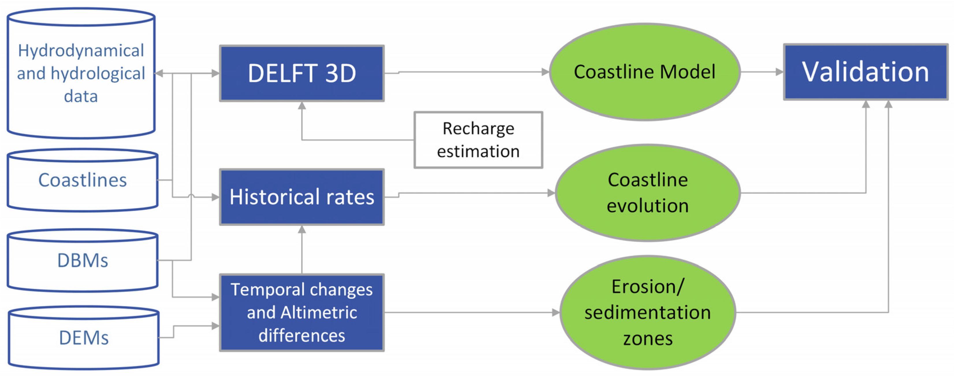
The inner bay of Deception Island is a collapse caldera with a flat bottom and steep walls, and thus its bathymetry is an important aspect of research on the island. In fact, this bay can almost be considered a lake, with important reception of tephra after eruptive processes [52,53]. In addition to this, the presence of submerged volcanoes such as the Stanley Patch volcano, the largest volcanic cone located in the southern sector of the bay [54], and the narrow entrance to Port Foster (Neptune’s Bellows, see Figure 1b) require precise bathymetry for navigation purposes.
The oldest digital bathymetry model (DBM) of this study was initiated and compiled by Spanish public institutions such as SGE/CGE, the Instituto Hidrográfico de la Marina (IHM), and the Instituto Español de Oceanografia (IEO) between 1988 and 1991 with an orthometric height from a local tide gauge reference and submetre differential GPS [43]. It was included in the CGE maps with 10 m bathymetric contours, the same as the level contours according to the printed scale of the map that was digitised in SIMAC. New Spanish bathymetry data from IHM were recorded in two different campaigns in 2012 [37] and 2016, compiled in an xyz file with an altimetric error of 0.5 m and 5 m for planimetry following the metadata information.
From the Marine Geosciences Data system (MGDS), seven subsets were downloaded with the descriptor “Sea depth (uncorrected, calc. sw sound vel. 1500 m/s) metres”. These subsets are from the Laurence M. Gould expedition (LMG prefix) between 2000 and 2009, and the points located in Port Foster were selected and combined into one GIS file (see Figure A1). Anomalous depth measurements produced by false return were identified using GIS tools (spatial outlier detection) and removed. Also, the 2006 itinerary around Walers Bay was not considered due to a flashing anomalous value in the temporal track. The final set had 17,256 points (11,289 only in 2000), and a mean grid was calculated using 50 m cells, the same resolution as that used in [55], with some of these files in the same zone. The grid date was set with 2005 as the mean year (MGDS mean dataset), and the mean standard deviation was 1.87 m with σ = 2.2 m. These values were not corrected for tidal effects, of which the maximum amplitude was 2.025 m [38,39], like the mean standard deviation. A similar value of 2 m was assumed for overlapping outer beams as that in [55]. In terms of positioning error, a positional uncertainty of 5 m can be considered, since it is very likely that, like the previous data, it was acquired with the use of a GPS differential. The navigation paths through the narrow Neptune’s Bellows suggest that this value is correct.
All input bathymetric data were transformed into EPSG 32720 and can be consulted in Table 3.

4. Methodology

The methodology employed in this study is described in Figure 3. It encompassed three primary processes: the establishment of a coastal numerical model, two GIS studies dedicated to finding and quantifying historical geomorphological changes (DEM and DBM alterations) and tracking coastline evolution for model evaluation.

4.1. Numerical Model

The model used in this study was DELFT3D, developed by WL|Delft Hydraulics, 237. It was implemented with a 2D (depth-averaged) configuration. This model solves the shallow water equations with Boussinesq and hydrostatic approximations [24]. The system consists of horizontal momentum equations, the continuity equation, the transport equation, and a turbulence closure model. The formulation used in the FLOW module makes it ideal for predicting flow in shallow seas, coastal areas, estuaries, lagoons, rivers, and lakes. It aims to model flow phenomena where the horizontal length and time scales are significantly larger than the vertical scales. The user can choose to solve the hydrodynamic equations on a Cartesian rectangular, orthogonal curvilinear (boundary fit), or spherical grid [24]. The continuity equation assumes incompressible flow and is defined as
u x + v y = Q
where u and v are the components of the velocities in the x and y directions, respectively, and Q indicates the mass transport per unit area.
Furthermore, the momentum equations are described by
D u D t = 1 ρ 0 P x + F x + M x + f v
and
D v D t = 1 ρ 0 P y + F y + M y + f u
where t is the time, ρ 0 is the reference density of the water, f is the Coriolis parameter, P x and P y represent the pressure gradients in the x and y directions, respectively (including barotropic and baroclinic terms), F x and F y are the horizontal Reynolds tensor in both directions, and, finally, M x and M y represent the contributions due to external sources, such as the wind action on the free surface or the wave action on the water column.
The model also incorporates morphodynamical evolution equations, which calculate the total transport as the sum of bed and suspended load transports. These transport rates are obtained using the depth-integrated advection–diffusion equation [62] for different sediment fractions [62], which can be cohesive or non-cohesive and are defined based on their densities and sizes. The calculation of bed shear stress uses the roughness predictor of [28]. The level of the bed is updated during each time step of the flow calculation, considering the exchange with suspended sediment transport and the gradient of bed load transport.
As field-measured data on actual river flows resulting from snow melt were not available, river flows based on the lengths of the different main waterways and the numbers of tributaries ( n o .   o f   t r i b u t a r i e s ) for each of these watercourses from their source to the discharge point were utilised. Since there is no known single experimental formula to estimate the flow derived from snowmelt, we developed our own formula to categorise the rivers according to the criteria described (lengths of the main rivers and tributaries), allowing us to estimate their flow Q m e a s u r e d in litres per second (l/s) and place possible values in the range of 10–100 l/s. The formula used to determine the flow rate in the rivers was as follows:
Q m e a s u r e d = 0.01   l / s   E n t i t y   + 0.01   l / s   n o .   o f   t r i b u t a r i e s 2
In this formula, the E n t i t y is a value between 1 and 5, depending on the total length of the main rivers up to the discharge point. To calculate the flow resulting from snowmelt ( Q t h a w ) , the following formula was used, using the parameter Q m e a s u r e d from Equation (4) and the b a s i n   a r e a of each stream:
Q t h a w =   Q m e a s u r e d     1000   b a s i n   a r e a   ( h a )

4.2. Coastline Evolution

Digitising changes in the inner coastline from last eruption period involved the analysis of orthophotos of 1968, 2003, and 2020 and the inclusion of a partial 1970 coastline from [48] within a GIS environment [63]. The methodology used (Figure 4) was also implemented through two different approaches: (i) assessment of area changes, and (ii) linear ratios.
In the first step, conducted in QGIS v 3.28 software [63], the linear coastline shapefiles were converted into polygons to delineate the intersection areas between the current shoreline (2020) and the preceding shorelines (1968, 1970, and 2003). These polygons helped with the identification of regions where erosion or sedimentation had taken place within the inner bay over time, allowing for a comparison with the results derived from the DELFT 3D model. The sediment plumes observed in the orthophotos were an important aid in accurately delineating the coastlines (see Table 1). A sediment plume refers to the visible cloud of suspended sediment particles in the water, carried by currents and tides. This approach often focused the analysis on slope alterations and retreats in specific areas of the island, such as the Spanish and Argentinian bases. This ensured that the visual comparison of shoreline changes, as derived from the generated shapefiles, corresponded with the transformations occurring within the inner bay of Deception Island.
In addition, DSAS v5 software was used to evaluate dynamic rates derived by comparing coastlines from 1970, 2003, and 2020 in a second step. This software is an ArcGIS extension [64] and a powerful tool specifically designed for the analysis and monitoring of coastlines using geospatial data [65,66]. Specifically, this application was used in this study to visualise and assess changes in the position over time and identify vulnerable areas. Coastline retreat/accretion ratios were obtained at specific locations, excluding areas that showed minimal changes in their position after the first step. For the calculation of these, DSAS uses cross-shore profiles, and the ratios were obtained by dividing the maximum calculated value of the coastline displacement within each of the analysed profiles by the time (in years) between the evaluated coastlines. As the 2003 coastline served as the baseline in the numerical model and given that this year was sufficiently distant from the 1970 eruption, we analysed two distinct time periods: (i) 1970–2003, capturing the impact of the introduction of new volcanological material, and (ii) 2003–2020, representing the ongoing trends in the bay.

4.3. DEM and DBM Temporal Changes

The DEM and DBM datasets in the ESRI GRID format were the input data in this section of our work. The temporal change methodology was carried out with GIS tools in the ArcGIS Pro environment [64]. Both datasets underwent the same procedures for change evaluation, except that the determination of the inner watershed was executed only for the DEM dataset. The GIS methodology is shown in Figure 4 and consists of four subprocesses: (i) calculation of altimetric differences with a study case in CR70, (ii) calculation of altimetric differences by range slope, (iii) calculation of volumetric differences, and (iv) a space time pattern study. In a previous step, the delimitation of the DEM study was defined using the determination of the inner watershed limit. Altimetric differences were used to identify areas of gain and loss in the temporal range. Slope classification was intended to assess the influence of positional error on these differences. Volumetric difference calculations allowed for the isolation of positional errors from elevations, elucidating the overall trend within the inner basin. This trend was spatially delineated via the statistical analysis of temporal studies. These studies helped us to understand the surface dynamics and their potential influence on, as well as material contribution to, the bay.
Calculating the altimetric differences by range slope required the altimetric differences as input data. Ascertaining these differences required an arithmetic operation, the main input data were the most current altimetric reading, from which the oldest reading was subtracted. The three slope ranges were divided to adapt them to the island’s morphology in land and water with breaks at 2° and 9°. This clearly grouped the most interesting study areas and potential erosion/accretion zones (e.g., beaches, abrupt relief, cliff, or caldera rims). The zonal statistics were derived using a polygon layer derived from this range of slopes.
We used some discrete altimetric levels, of −150, −100, 0, 100, 200, 300, and 400 m, for the evaluation of volumetric differences. These datasets did not have a specific capture date. For SIMAC DEM, 1986 was used as the collected date, corresponding with the DEM information for most of the surface. REMA was assigned 2015 as the middle year, and for the same reason, 2014 was assigned for IHM DBM (see Table 2 and Table 3). In addition to this, the DEMs retained their original spatial resolution (2 or 2.7 m), while in the case of DBM, two new resampled raster files with a new resolution were used (IHM DBM 50 m and SIMAC DBM 50 m). Annual ratios per unit of 3D area were computed to obtained comparable values.
The space–time analyses highlighted the trends with statistical significance over time. Three were conducted, one with DEM and two in the DBM dataset:
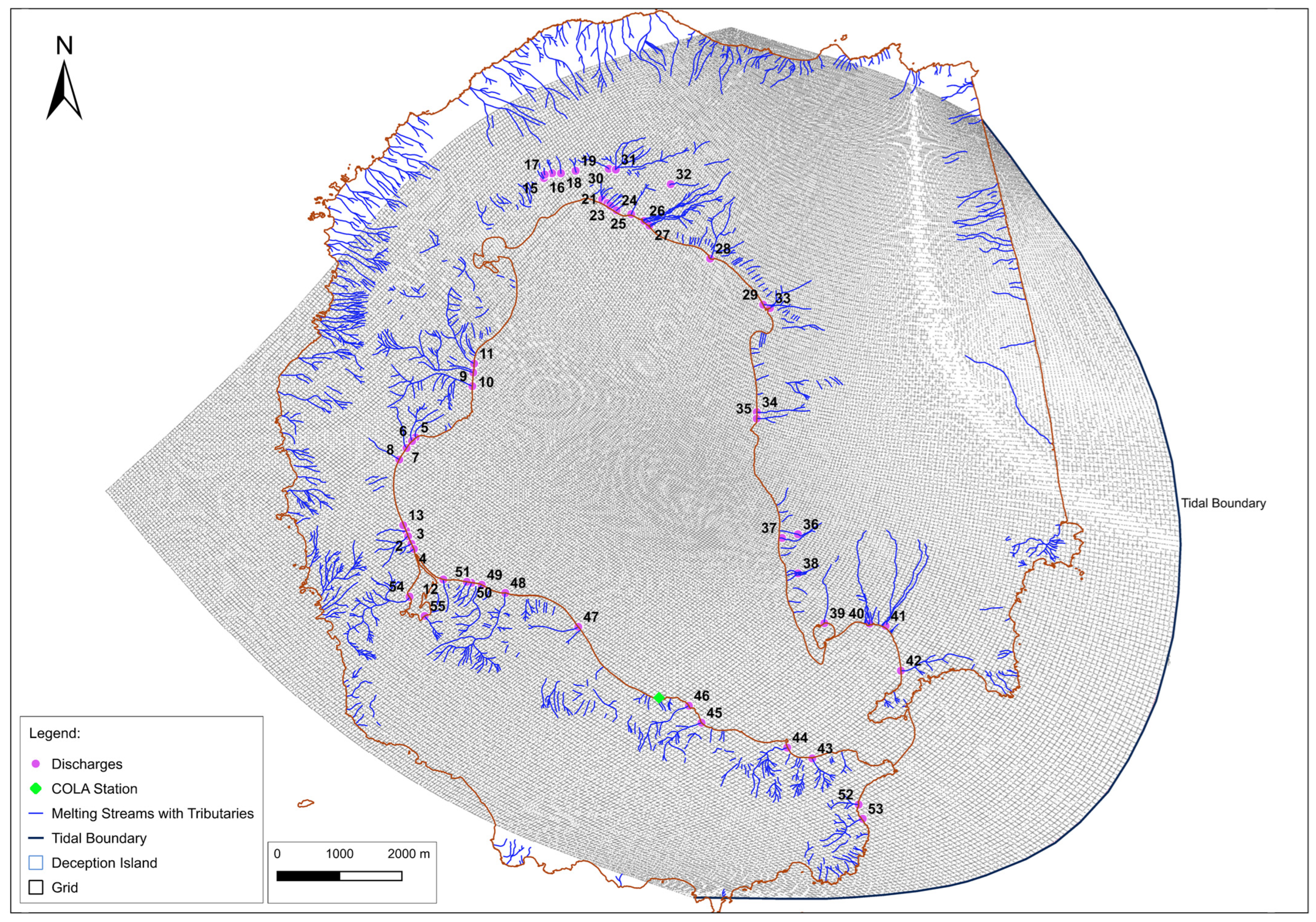
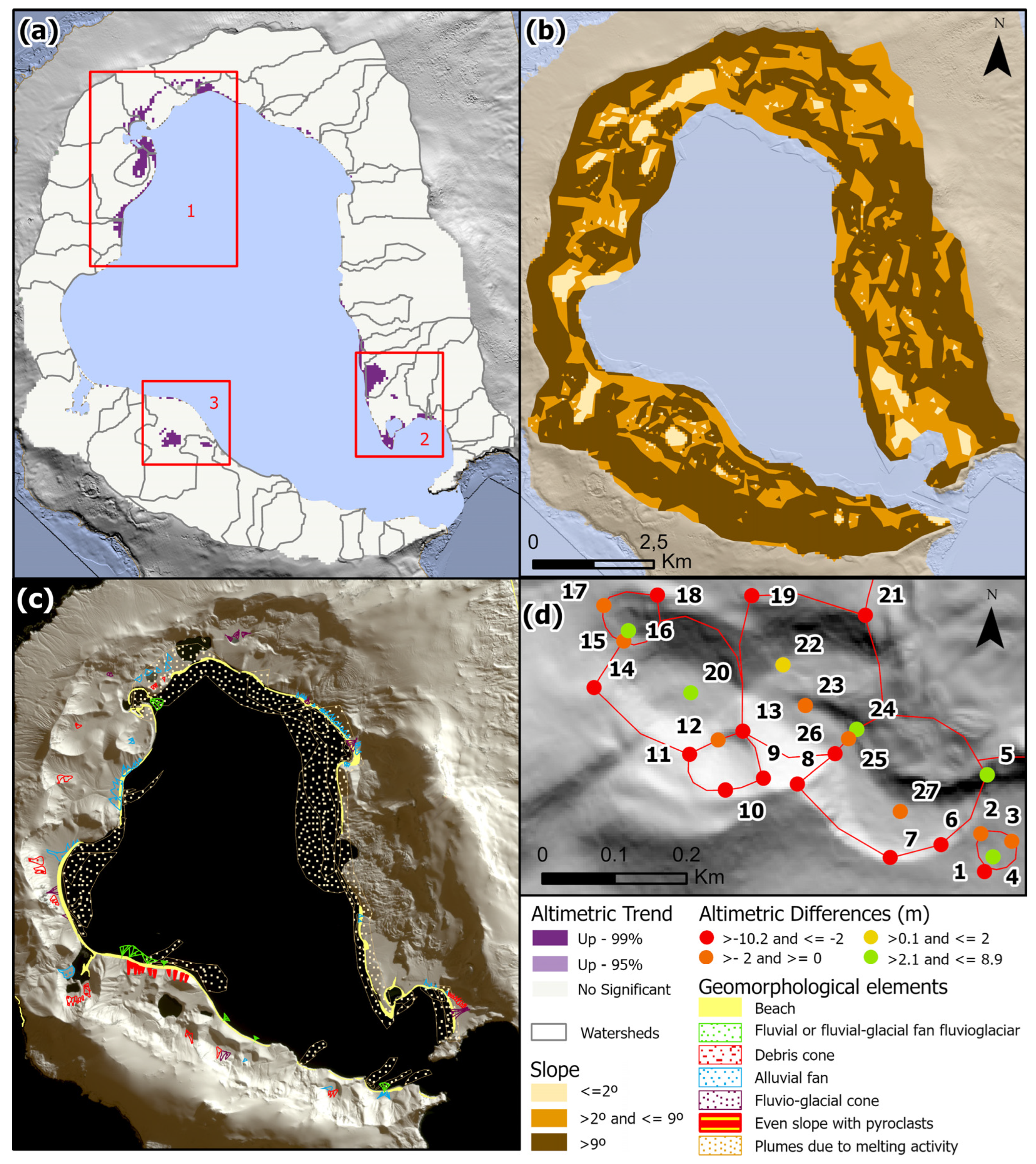
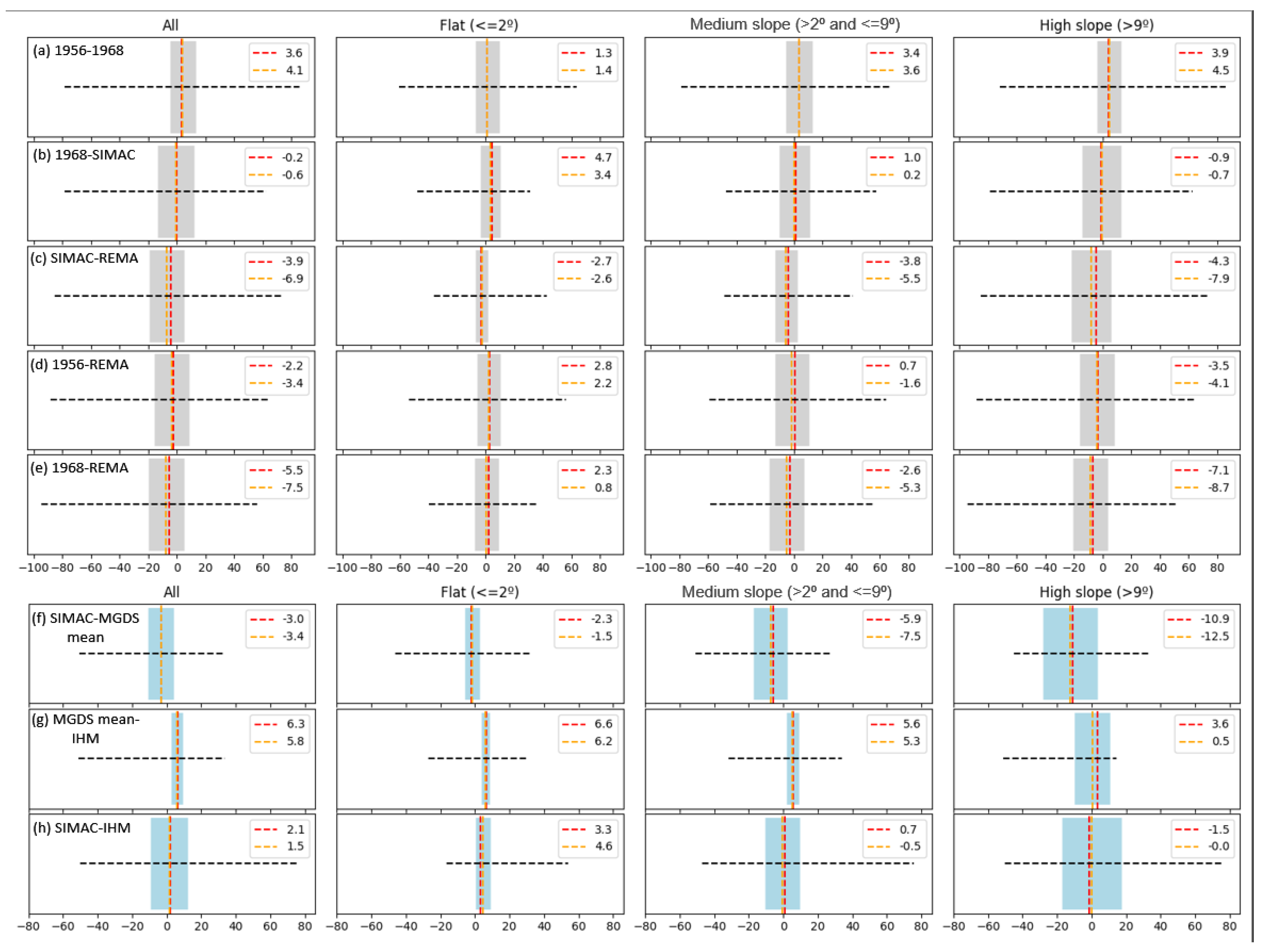
  • The DEM space–time analysis started in 1956 (including the last volcanic event) and used a 1-year time step to cover DOS DEM (1956) and its own 1956 DEM. We used a 50 m resampled DEM and a cubic technique to decrease the planimetric and altimetric errors. The space–time cube aggregated 73,073 points into 46,368 fishnet grid locations covering 64 years.
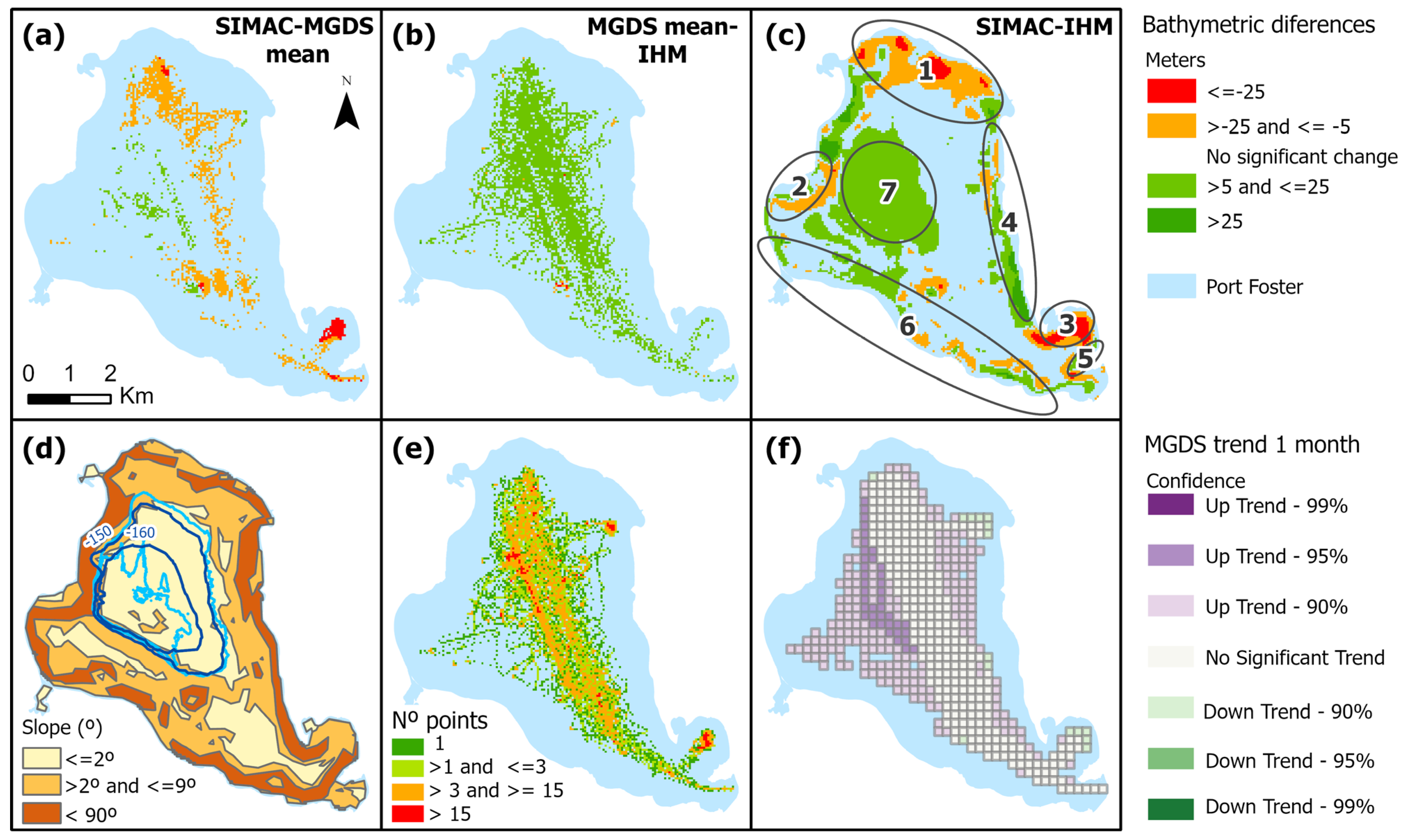
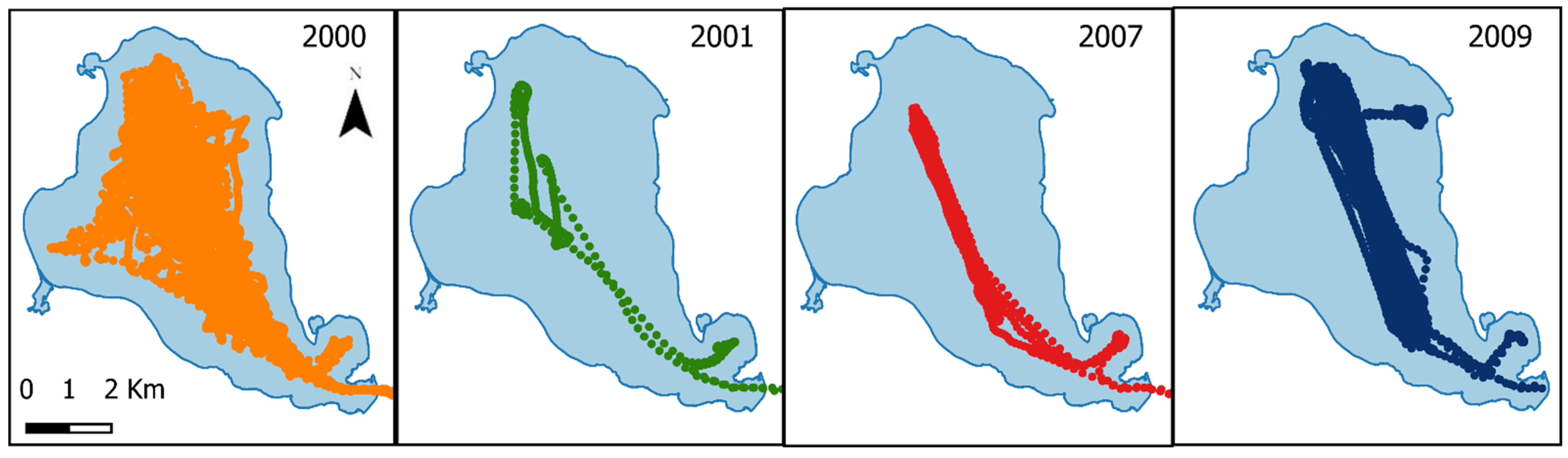
  • The DBM dataset included two data structures, for which we aggregated points into space–time bins: (i) only MGDS data (19 November 2000 to 29 March 2009) in a 1-month study, with 17,256 points aggregated into 1560 fishnet grid locations and 200 m of spatial resolution used to increase the numbers of points so that there were several points in the same cell, and (ii) using the original resolution of the SIMAC DBM, IHM DBM, and External South Shetlands DBM in a unique point layer and including the MGDS mean layer in the same format (see Table 3). This last study used a 1-year study, 200 m of spatial resolution, and 10,032,219 points aggregated into 2601 fishnet grid locations over 28 years.
A last point to note concerns the error margins in these calculations. Altimetric differences were influenced by positional and altimetric errors and the propagation of both into the arithmetic operation. The superficial and volumetric error was simplified to the error associated with the determination of the 1 hm3 box.

5. Results

5.1. Numerical Model

5.1.1. Model Setup

The model domain was defined as a computational curvilinear grid (Figure 5), with a total of 731 × 731 cells and a maximum resolution of 15 × 10 m2 within Deception Island. The initial conditions of the simulation were the values obtained with field measurements during surveys carried out in 2012 (for more details, see [38]), avoiding cold starts; the inner bay bathymetry in the model that from the SIMAC DBM (Table 3); and the closest coastline, temporally speaking, the 2003 coastline (Table 1). The year 2003 was sufficiently distant from the 1970 eruption to reflect the ongoing trends in the bay. Meanwhile, the outer open-sea bathymetry, representing the areas beyond the coastline, was covered by the External South Shetlands DBM (Table 3).
River discharges were modelled to occur during three months of the year (January, February, and March), and we simulated the actual situation of snowmelt on the island, which is frozen during the rest of the year. The mobilisation of all sediments deposited during these three months within the inner bay leads to erosion or sedimentation of the inner coast. The number of tributaries varied between each river (considering tributaries with a minimum appreciable length), and the lowest assigned flow was 10 l/s while the maximum was 95 l/s. Table A1 in Appendix B shows the modelled characteristics for each discharge in terms of river flow.
The boundary conditions (tidal boundary in Figure 5) of the free surface are given by the nine principal astronomical components (semi-diurnal and diurnal constituents) [67] as M2, K1, O1, S2, P1, Q1, K2, N2, and MF, obtained from data observed during field surveys [38,39,68]. More information about the meanings of these parameters can be found in [69]. Wind and atmospheric pressure conditions with a 1 h interval were obtained at a meteorological station during the same tide level survey [39,68], and those were introduced with a constant value for the entire grid.
Like previous studies [24,70,71,72,73], the morphodynamic module was found to be sensitive to the mean diameter of the sediment. According to data provided by field surveys in the area [34], a single sediment was defined, which was a silt due to its prevalence across 85% of the island. In agreement with an earlier work [74], the suspended bed load and suspended sediment transport factors were defined as 1 and 0.5, respectively. Considering the numerical constraints of the model (Courant number), the time step was defined as 0.1 min. In addition, a spatially uniform time-varying wind field was defined throughout the spatial domain with hourly data from the Spanish Meteorology Agency (AEMET).

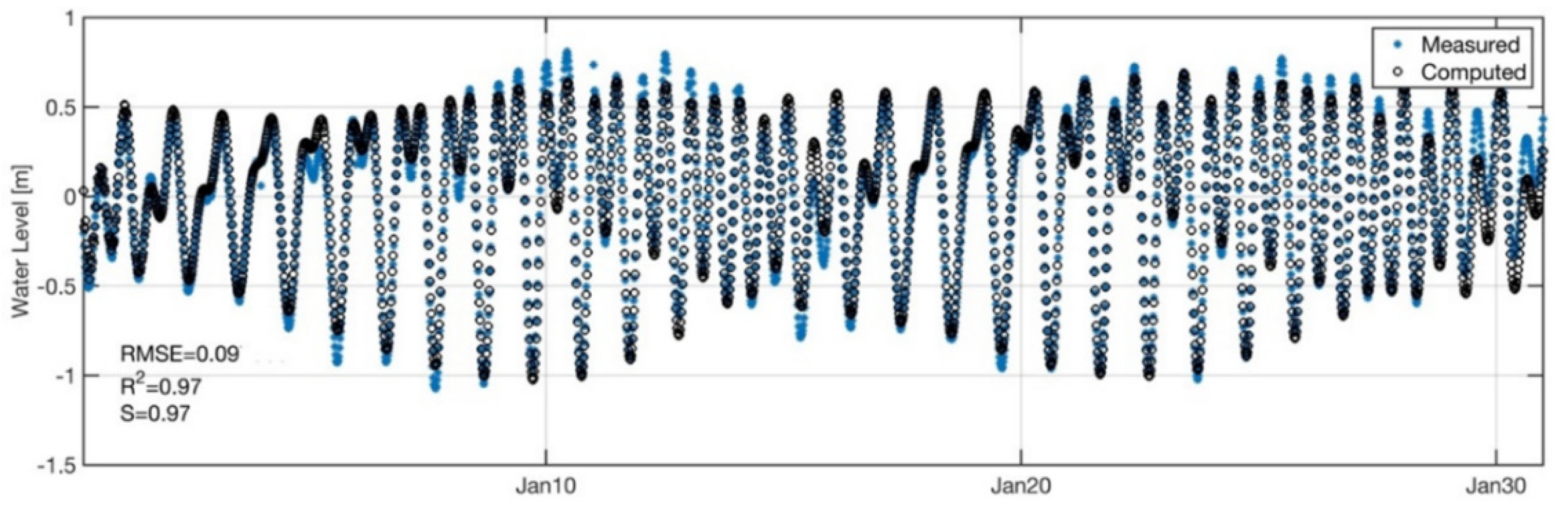
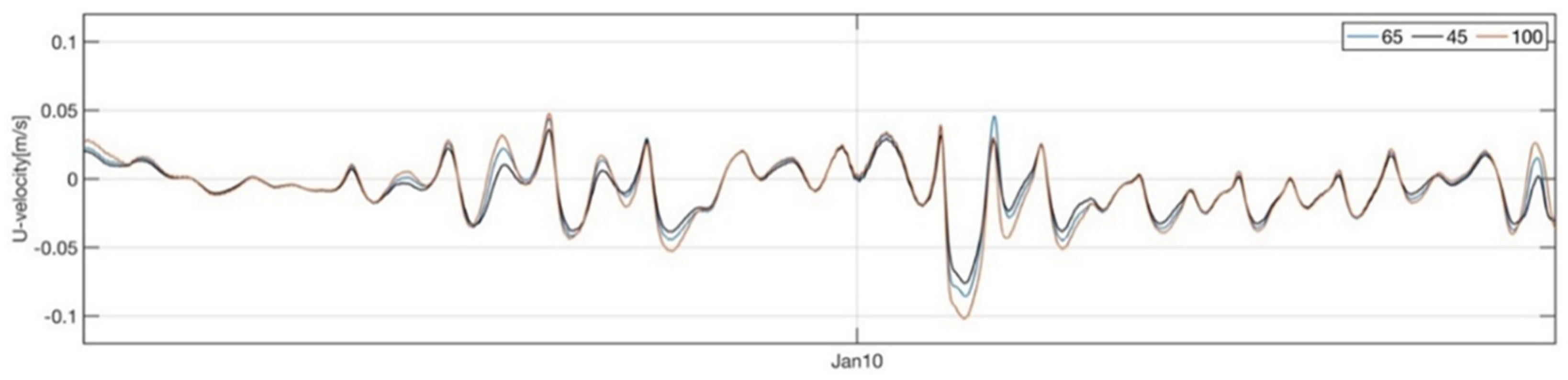
5.1.2. Model Calibration

The model was calibrated for the water level variable and for the harmonic components of the velocity (M2 and K1), both amplitude and phase. The water level data were obtained from the field survey conducted in 2012 (COLA Station in Figure 5), and the data for the harmonic velocity components were compared with the results of previous studies [39,68]. The full month of January 2012 was selected as the calibration date because it was a month where there was no lack of data and there were average meteorological conditions. The results are shown in Figure 6, where it can be observed that the agreement is excellent for the water level, obtaining values of R2   0.98 and skill coefficient  0.97.
In the case of velocities, the results shown in Table 4 were obtained. The phases values are correctly represented with a correlation coefficient (R2) of 0.9; however, the amplitudes are not correctly represented, varying by one order of magnitude from those obtained in previous studies [68]. Therefore, it was decided that we would evaluate different values of Chèzy (45, 65, 100) to perform a sensitivity study. Figure 7 shows how when changing the Chèzy coefficient, the values do not vary by more than 30% in the peaks, and in the rest, they follow a trend with a maximum variation of 3%. When the values of the amplitudes of the M2 and K1 components were calculated, the values were close to each other, varying by 4%. Therefore, we surmised that the results obtained with the numerical model were correct, and although it was not possible to give a final value of the sedimentation rate, it was possible to define sedimentation patterns by determining the accretion and erosion zones.
Once the model was calibrated, a full year (January 2012 to January 2013) was simulated with the same forcings described in the earlier section. The results are shown in Figure 8, which includes six zones studied in detail throughout this paper. This image illustrates that erosion along this coastline is particularly notable in areas with a southern orientation, such as zones 1, 2, 3, and 5. Sedimentary action tends to be concentrated along coasts oriented to the west (east shoreline, zone 4), northeast (south shoreline, zone 6), and east (west shoreline, up zone 2). The bathymetry and coastline used at the beginning of the simulation are based on data from 2003. This means that regardless of the specific date chosen for the simulation, the initial conditions for the bathymetry and coastline remained consistent and reflected the characteristics observed in 2003. That date was 33 years after the last eruption of the island, and as we understood it, there was no further input of material in the intervening period, so we expected no material other than that which already existed from the eruption.

5.2. Coastline Evolution

In line with the methodology described in Section 4.2, Figure 9 illustrates differences over two distinct time intervals (1970–2003 and 2003–2020) using the initial year of the numerical model as a breakpoint. The figure depicts accretion and erosion using polygon areas (green for gain and yellow for loss) and annual regression lines from DSAS v5 software (negative regression in red and positive in blue).
During the first period (1970–2003), reflecting the impact of new volcanological material, there was a water area increase of 0.77 km2 primarily due to erosion and the inclusion of Kroner Lake (Figure 8, zone 3), while decreasing by 0.23 km2 due to sedimentation along the shoreline. In the next period (2003–2020), considered the prevailing trend, the interior water area of the bay expanded by 0.48 km2, encompassing the opening of “Lago Escondido” (zone 1) and glacier retreat (zone 4). Also, it decreased by 0.05 km2 due to sediment movement. The annual ratios for bay area increase were near-consistent, at 0.023 km2/year and 0.028 km2/year in the two periods, while land area decreased from 0.007 km2/year in the first period to 0.002 km2/year in the second.
The profiles analysed using DSAS v5 software were superimposed, with color-coding showing the intensity of the annual coastline evolution ratio in corresponding areas. It should be noted that the opening or addition of crater lakes was not represented in this calculation. While in the first period, the erosion values in the northern and western regions were 6–9 m/year, with a slight retreat in the southern coast with 0.3–2 m/year, the second offered a reduction in the intensity. In particular, notable erosion was clear in the northern and northwestern parts of the island (with the same value of 0.3–2 m/year), as well as in the south, where the Spanish and Argentinean bases are located. The significant retreat experienced by the Negro Glacier was noteworthy, which increased its annual retreat to 14 m in the 2003–2020 interval compared to the 7 m/year it experienced between 1970 and 2003, representing a 100% increase in its annual retreat. Regarding sedimentation, areas located at the ends of the Black Glacier saw a coastline advance of approximately 150–200 m in the south and 50–100 m in the north. This progress was halted in the second period analysed. Other areas that were less prominent in terms of coastline advance during the first interval experienced inverse changes in the second period, even showing a retreat in their values like sedimentary areas in the southwest of Port Foster (west of zone 6) and to the northwest of the bay (north of zone 4) up to the aforementioned value of 0.3–2 m/year.
Figure 10 presents some zoomed-in images of the most notable gains/losses observed when we performed a visual analysis of the coastlines following the denomination in Figure 9a. These show the main changes that occurred in the western part of the island, specifically at the Black Glacier due to retreat (Figure 10a1–a3, zone a in Figure 9a), and its southern region (Figure 10b1–b3, zone b in Figure 9a). Additionally, they show the erosion of the slope in front of the Spanish base (Figure 10c1–c3, zone c in Figure 9a) and part of the erosion in the northern area of Port Foster (Figure 10d1–d3, zone d in Figure 9a). Zone d presents great sedimentation action produced by water and ash slides during the last eruption period in the observed inlet, too.
In regard to the precision of these values, we quantified the error in the linear values and introduced a need to have 2 pixels to identify an object. Using a 1 m resolution, which encompassed all the orthophotos, the average error for each linear measurement (two points) was set at 2.8 m. The error in linear ratios corresponded to the linear error derived from the definition of their profile line divided by the square root of the years of the studied period. When establishing the margin of error in surface determination, we simplified the former approach to the error in 1 ha of its bounding box coordinates, following the law of variation transmission [75]. Accordingly, the surface error was assessed at 28 m2/ha. All the provided figures are given in decimal units above the unit of error in this section and in later sections.

5.3. DEM Evolution

5.3.1. Inner Watershed

Following the GIS methodology of Figure 4, after the determination of the new inner watershed from REMA, temporal altimetric variations were calculated and are depicted in Figure 11, spanning the six decades from 1956. The upper panels illustrate the evolution over successive time intervals, whereas the lower ones delineate these temporal segments from the two newly studied older DEMs (1956 DEM and 1968 DEM) to the most recent one (REMA). Note the prevalence of green areas in Figure 11a,b, particularly around the sites of the most recent volcanic eruptions (Figure 11a, zones 1 and 2), which is contrasted by the loss of red in zone 2, signifying floods of molten water released from the glacier due to the opening of subglacial vents and the partial melting of the ice cover [15,36]. In particular, the areas covered by ice (inside the white line) exhibit the most significant and dynamic differences. These aspects are particularly pronounced in Figure 11c,e. Snowy areas are complicated surfaces to position altimetrically in the photogrammetric process, as can be read in a note written on the printed GCE map [44]. To the lack of control points is added the thawing periods making possible the high figures found.
The error of these differences was established via the quadratic composition of their sum [75], evaluating each surface at 4 m based on rounding its worst positional error value (2.7 m) to about 5.6 m, while excluding values ± 5 m in the representation.
The findings of our temporal trend study are shown in Figure 12a, with only three uptrend zones, one related to the last events of the 1969 eruption [30] (red rectangle 1 of this figure) and two representing gain zones (rectangles 2 and 3). Rectangle 2 is on the shoreline and was commented on in the previous section, and rectangle 3 corresponds to two lakes so that area was not taken into consideration. The global trend statistic is −0.097 with a trend p-value of 0.922. There is no statistically significant increase or decrease in the other zones over time.
These differences were classified additionally using slope ranges suitable for defining the different geomorphology of Port Foster and for controlling the influence of the positional error. The results of our statistical evaluation are presented as boxplots in Figure 13 using a row for each temporal difference and showing values for all the studied area (All), flat zones (≤2°), medium slopes (>2° and ≤9°), and steep slopes (>9°), as defined in Figure 12b. General mean negative values (column “All”) are present in all differences studies except for 1956–1968. Flat areas exhibit the smallest standard deviation values (light grey box), as expected, compared to the largest for steep terrain. The difference between 1956 and 1968 was calculated using the new DEMs, which were generated using the same control points. These DEMs showed similar positional errors, with a stable standard deviation in row a, despite including variations corresponding to the 1968 eruption. The rest of the results reflected the increase in slope and height variation due to this positional error. It should also be noted that the largest temporal differences in relation to REMA showed material gains in flat areas, while losses occurred in steep areas.
The volumetric values, temporal evolution, and annual ratios for 3D areas of the digital models are shown in Table 5. The volume was calculated by moving the reference plane 100 m upward in each DEM. Table 5 includes the difference with respect to the same plane defined in the previous temporal model (“Dif. Vol.” column) and a temporal and spatial ratio value based on the provided 3D area. Except for the period that includes the most recent eruption (1968 DEM and SIMAC DEM) with a gain of 0.19 km3, the remaining DEMs show losses. The negative ratios in the last three DEMs were reduced from −0.50 to −0.23 hm3, and higher loss values were detected at elevations exceeding 300 m, associated with snow and, therefore, representing volume losses not related to the terrain itself. Ice melt activity is significant on the island and generates extensive sediment plumes, as delineated in Figure 12c from satellite images. The volumetric error for each 1 hm3 was estimated at 0.03 hm3, and for annual ratios, this error was divided by the square root of the years of the study period, following [75].

5.3.2. CR70

In 2006, 27 points were measured with subdecimetre differential GPS to define the dimensional characteristics of the 1970 craters (see Figure 2a1,a2). These new craters were evaluated in [34] and some infill rates of up to 1.5 m/year were calculated on the floor. Here, these measurements were compared with REMA using ellipsoidal height (thereby eliminating the uncertainty in the value of the geoid undulation), and the results are shown in Figure 12d and Table A2. The floors present increased heights (colours yellow and green), in coherence with the visual analysis of the 2020 satellite image and REMA hillshade in the background. In contrast, the inferred rims of the craters have loss, probably due to the lower planimetric/altimetric precision of REMA DEM compared to GPS or an erosion effect on the crater wall. The absence of a specific date for DEM values (2009–2021) makes it impossible to establish an exact rate. However, the altimetric gain was approximately 9 m in crater number 6 (Figure 2a1), which is fully filled according to the 2020 image. Craters 2 and 3 gained 6 m and 2 m, respectively, with a notable rise at the floor due to the active displacement of material uphill from the Mount Goddard alluvial fans. Unfortunately, the 52 GCPs used in the orthophotos could not be used to validate the altimetric changes in the terrain because they were located on the rooftops of the stations’ buildings or on rocks. The error in these altimetric differences was assessed based on the error derived from REMA at 1 m, as the GPS derivatives were established at 4 mm [34].

5.4. DBM Evolution

The DBM range differences are shown in Figure 14 and cover more than 50 years. The error associated with the BDMs was valued at a mean value of 3 m, which, by variance transmission, provides a threshold of 4.3 m to the difference. This value was disregarded in the graphic representation and raised to ±5 m to assimilate its study to that shown in Figure 11 with the DEMs.
As shown in the first line of images in this figure (Figure 14a–c), surprisingly high values of altimetric differences were found again. The most extensive area with an increase in height (Figure 14c, new studied zone 7) was the bottom isobath of 150 m, and the sea bottom was almost featureless and flat below this depth (see Figure 14d). Losses were mainly concentrated in the studied zones 1 and 3, which are closer to the shoreline.
These differences were classified using slope ranges that were suitable to define the different geomorphologies of the bay and to evaluate the influence of positional error (Figure 14d and Table 5). The altimetric reference seemed better in the case of MDGS and IHM bathymetries, with a standard deviation of 3.4 m and a global sedimentation (mean gain of 5.8 m and high value of 6.2 m in flat areas). The global study from 1991 to 2012 (Figure 14c) had a clear positional error compensating in the ranges shown in Table 5. In this way, the mean difference in medium and high slopes decreased with increasing slope, while the standard deviation increased, too. As in the DEM study, high values were associated with steep terrain (dark brown in Figure 14d).
Volume was determined by shifting the reference plane 50 m downward in each DBM, and the results are displayed in Table 5. In this case, the volume corresponded to the water, not the land; therefore, the reference is ‘BELOW’. The overall volume of the bay increased, and from the bathymetric elevation of 150 m onward, it increased while showing clear bottom sedimentation. The volumetric error for each 1 hm3 was estimated at 0.03 hm3, following [75].
Lastly, the space–time trend analysis using MGDS data (Figure 14e displays a heat map with the number of measurements) exhibited statistical significance only in specific areas, as illustrated in Figure 14f. These significant areas are found primarily in shallower, flat seabed, and correlated with sedimentary regions, as can be seen in Figure 14c. Unfortunately, the second study, which encompassed all bathymetric points, did not produce zones that displayed statistical significance over time. Evidently, the data’s precision (exceeding 1 m) and certain height uncertainties influenced the results of this second spatio-temporal analysis.

6. Discussion

Figure 8 shows the coastal variations between the start and end of a simulation year. Since currents were not precisely calibrated, erosion and sedimentation rates may not have been very accurate. However, trends of gain and loss patterns could be examined and corroborated using historical studies. Figure 8 illustrates a pronounced correlation between shoreline orientation and erosion or sedimentation. Based on this criterion, six study zones were delineated and included in Figure 8, Figure 11a, and Figure 14c: Zones 1, 2, 3, and 5 exhibit a southern orientation and are associated with loss action, while Zone 4 has a western orientation and Zone 6 has a northeastern orientation, both linked to gain action. Also, for DBM studies, a Zone 7 was included in the deepest part of Port Foster.

6.1. Coastline Evolution

The coastline study revealed erosion values greater than those for sedimentation. In detail, its zonal comparison with the proposed model followed the same trend in these points:
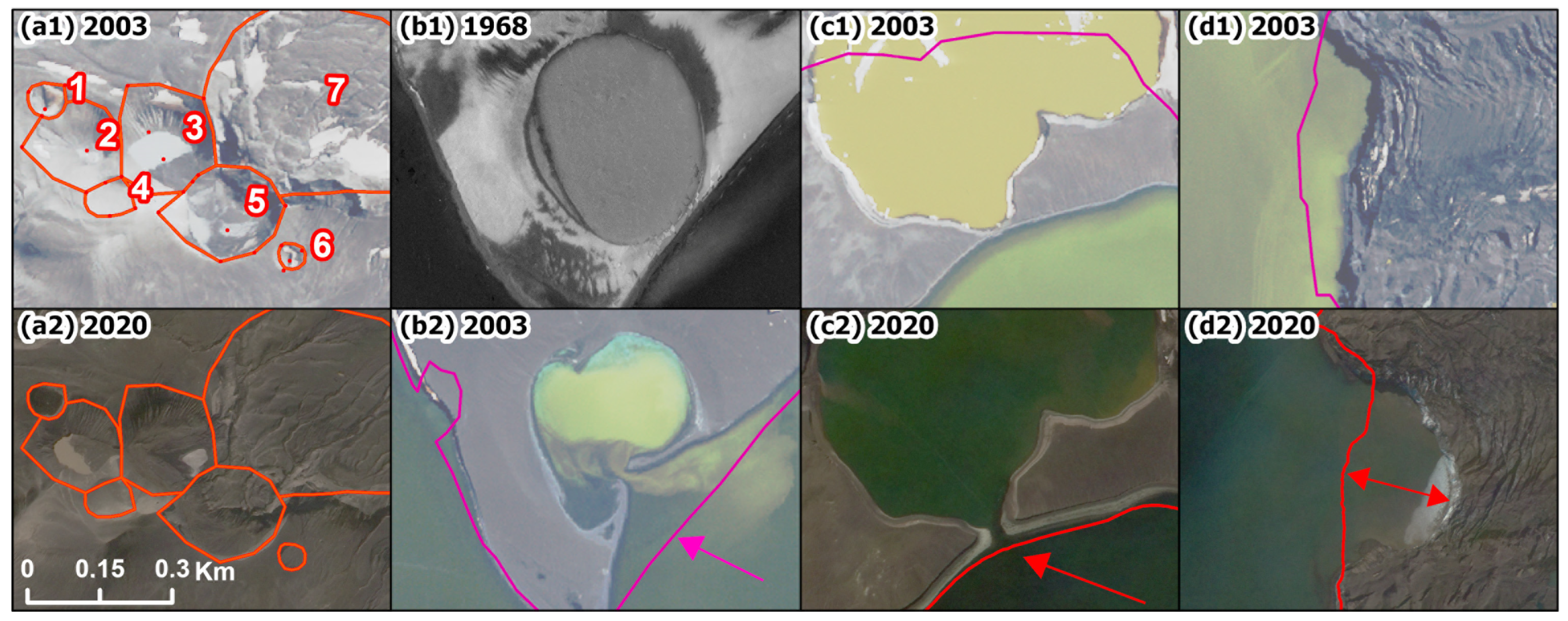
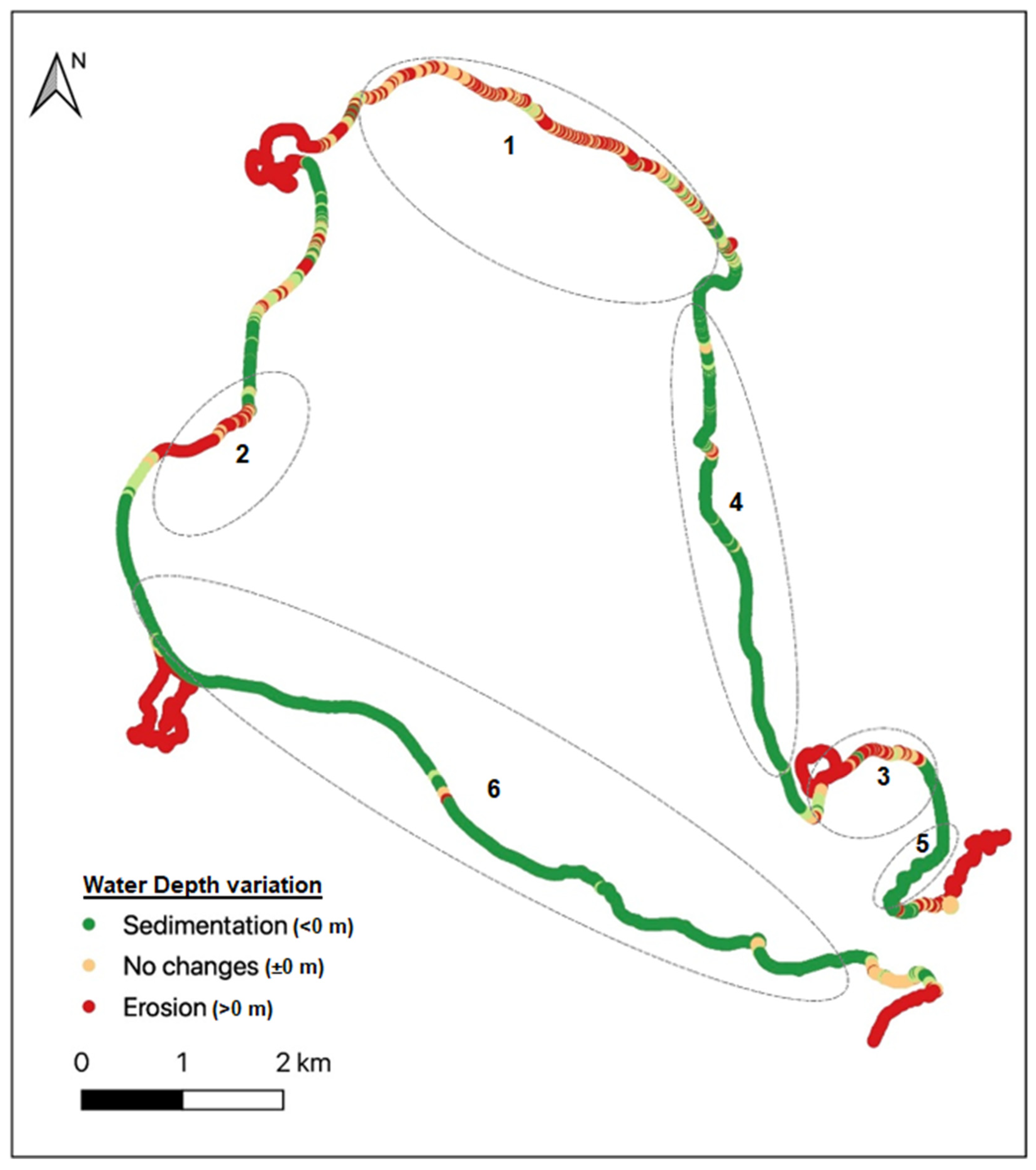
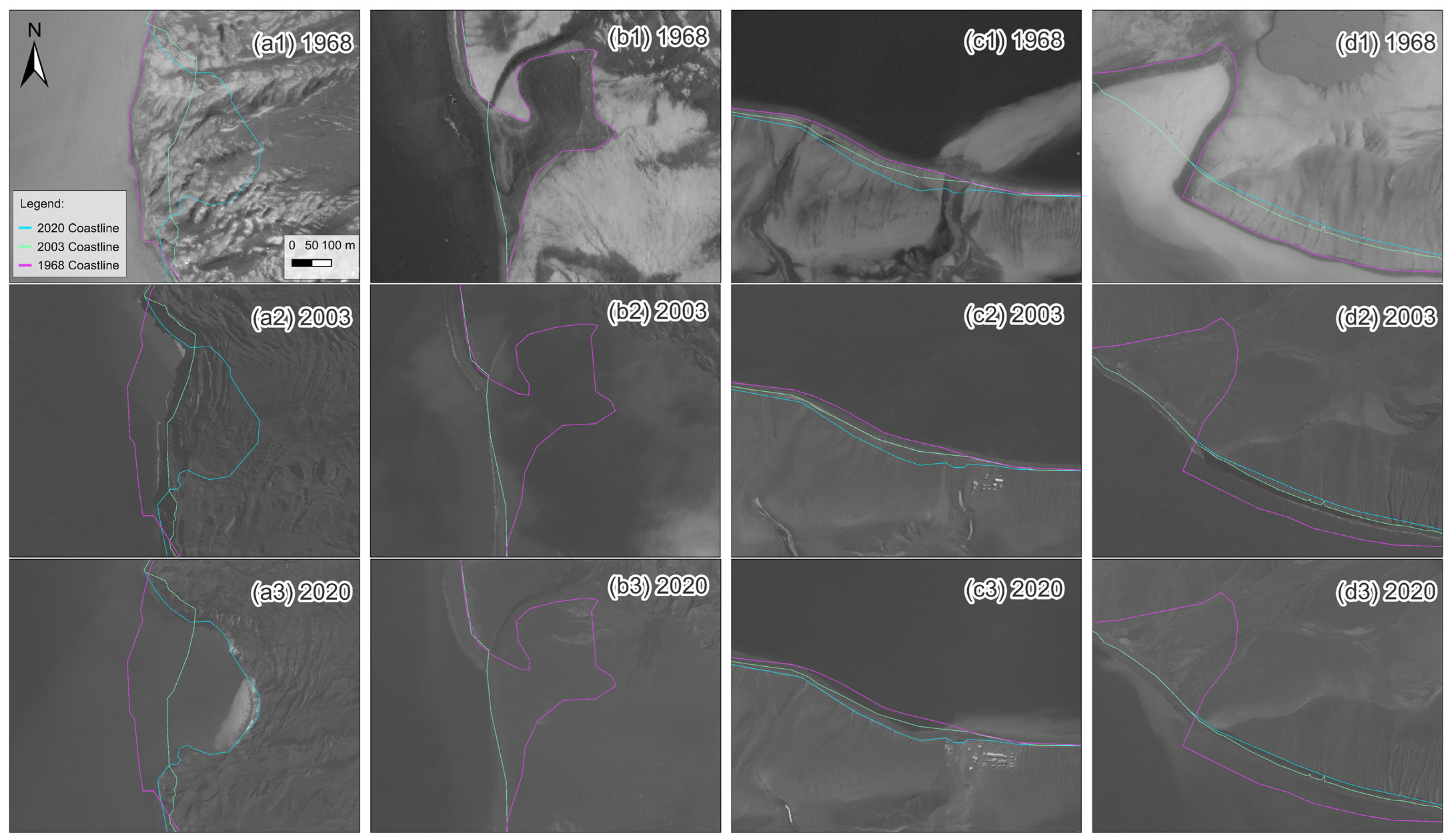
  • Zone 1: There was significant erosion in this zone since the last eruption, especially up to 2003, when there was significant erosion due to the transport of materials deposited after the eruption. Also, between 2003 and 2020, there was a notable change, which was the opening up of “Lago Escondido” (Figure 2c) due to the erosive effect.
  • Zone 2: This zone did not experience coastal retreat after 2003, but it occurred prior to 2003.
  • Zone 3: A similar effect as in Zone 2 was observed in Kroner Lake (Figure 2b).
  • Between Zone 1 and Zone 2, the model revealed erosive initiation that was also detected in the historical study.
  • Zone 4: Although predominantly sedimentary until 2003, there was a substantial accumulation of sediment in the southeastern part, following the termination of the Black Glacier (see Figure 9a and Figure 10b). This was the effect of floods of molten water released from the glacier due to the opening up of subglacial vents and the partial melting of the ice cover in the last volcanic period [15,36].
The discrepancies were in the following points:
  • Zone 4: Although this zone clearly saw sedimentary action, there was a clear inconsistency with the model. On the one hand, there was the glacier retreat that was clearly identified in the historical study (Figure 10a), but this was probably not due to the bay dynamics; instead, it may have been linked to global warming [22,76].
  • Zone 5: This zone showed no trend following on from the historical data, despite being clearly defined as sedimentary in the model. The proximity to the boundary conditions of the bay and, therefore, of the model or the need for a longer time to clearly reflect sedimentation values may have been the cause.
  • Zone 6: In the south of Port Foster, where the historical study represented the erosion produced on the slope in front of the Argentine and Spanish bases (Figure 10c), the model showed a sedimentary zone. We believe this slope erosion to have resulted from the impact of the sea ice fragments left by the bay’s melting and accumulating in this area against the weak volcanic material. In this sense, it was confirmed that the area had a sedimentary trend due to its current dynamics, but other effects that had not been considered were active and predominant in the area. Also, the numerical model presented a limitation in accurately evaluating erosion caused by snowfall on the slopes, particularly when the surfaces of slopes were elevated compared to the coastal shoreline. The annual snow melting process can lead to slope erosion as the melted snow water flows over the slopes and transports sediment, gradually washing away the exposed surfaces. Since the numerical model may not have incorporated detailed representations of snowmelt erosion processes, it may not have fully captured the erosion seen in the field. Snowmelt erosion is influenced by various factors such as slope gradient, surface characteristics, and snowmelt patterns, which are challenging to simulate accurately in a numerical model.
It is also interesting to note that the erosion rates in the areas not affected by the eruption in the first stage studied (southern coastline) were like those found in the second stage on the eroded cliffs along the whole bay, with values of 0.3–2 m/year. Another observation was that the erosion detected by the model within various lakes (e.g., Kroner Lake in Figure 2b1,b2 and inland intrusions (northwest of zone 6) may have been influenced by multiple factors. In addition to the influence of tides and simulated sea-level variations in the model, these areas had river discharge points where the flow resulting from snowmelt was transported. This created zones where there was interaction between sediment deposition and its collection by the tides, which then transported it to other areas of the bay. As a result, part of the sediment tended to accumulate at the lakes’ exits. These areas require a more refined modelling approach, and fortunately, we cannot offer decisive findings regarding them in this study.
Finally, it should be noted that when analysing the evolution of the coastline from images, the presence of shadows can pose a challenge, even when using high-contrast images. Shadows can obscure and distort the coastline, making it difficult to accurately define its boundaries. It is important to consider the impact of shadows when interpreting and analysing coastline changes, as they can affect the accuracy of the results. Techniques such as image enhancement and careful manual interpretation were employed to mitigate the effects of shadows and improve the precision of coastline delineation.

6.2. DEM and DBM Temporal Changes

The contrast between Figure 8 and our DEM analysis left only a few reliable values along the coast, which revealed some consistencies with the model in terms of sedimentation south of zone 4 and erosion in zones 1 and 2. In the DBM analysis, this showed a coherence between the most eroded shoreline and the nearest seabed in zones 1, 2, and 3. In addition to this, the sedimentation areas were also similar, with notable infilling occurring between the 1970 eruption and the year 2003 in the southern part of the Black Glacier. The most extensive area with an increase in height (Figure 14c, zone 7) was the bottom isobath of 150 m, where the sea bottom was almost featureless and flat below this depth (see Figure 14d). This area was studied by Cooper et al. [33] with shallowing rates of up to 0.3 m/year from 1829. In the data in Table 5 from the bathymetric elevation of 150 m onwards, it increases, showing clear bottom sedimentation.
According to this table (Table 5), the DEM loss volume is significantly greater than sedimentation in the bay. By adjusting the reference plane, this study revealed that the highest loss ratios occurred in the upper areas that were permanently covered in snow. Consequently, it can be understood that most volumetric loss was due to snow. Furthermore, the positive evaluation of the inner watershed in the period of 1956–1968, including part of the last eruptive process, was 0.19 km3, and the volume of erupted ash totalled between 0.12 km3 [77] and 0.20 km3 [30], with 0.10 km3 more recently [32] given as a possible figure. In addition to this, the area of the temporal sedimentation plumes drawn in Figure 12c shows a continuous and high active discharge of tephra according to zones 4 and 6 in the model. The material loss ratios have been decreasing since the last eruptive process, although they stay relatively high. The evaluation of the study case in CR70, revealing filling of most of the area (see Figure 12d) due to the active displacement of material uphill from the Mount Goddard alluvial fans, provides a sample of this activity and demonstrates the possibility of high sedimentation rates in certain areas. Volumetric changes in DBM indicate the loss of material from the steep walls of the caldera, some of which will accumulate on the sea floor. However, there must be a transfer to the outer part of the bay to balance the losses and gains.

6.3. Numerical Model

Following the validation of our model, we compared it with other studies on Port Foster dynamics:
  • Flexas et al. [37] found that temperature gradients across Neptune’s Bellows, driven by the Bransfield current, cause water to accumulate at the northeast entrance of Port Foster. They proposed that counter-clockwise-propagating internal tides create shadow areas on the bay’s eastern side, aligning with our model results in Figure 8.
  • In a study by Berrocoso et al. [40], they explored the connection between the distribution of water temperature in Port Foster Bay and the island’s seismic and volcanic activity. They suggested a link between increased seawater temperature and the resumption of volcanic hydrothermal activity. Their water circulation model over tides, with cold water entering the bay and mixing with warmer water, corresponds to our erosion patterns in the northern part of the island.
  • Figueiredo developed a hydrodynamic model [41,42]. His simulation showed limited particle exchange between the bay and its surroundings over one month, contradicting our observations of significant material displacement and sediment accumulation in the eastern area. The discrepancy may be due to the short simulation period in this study of only one month, making it difficult to draw significant conclusions.
In summary, these comparisons show that our findings align with some previous studies but differ from others, suggesting the complexity and variability of Deception Island’s coastal dynamics. At the close of this discussion, it can be concluded that the model simulates reality well and can serve as a future tool to chart the depositional trends of the study area. If this model is maintained over time, the evacuation routes (Figure 1b) along the inner coast and the accessibility to active scientific bases will not be affected except for by the recession due to erosion identified on the slopes in front of the two bases, which could impede access as the altimetric difference between the beach and the terrain increases.

7. Conclusions

In this study, we developed a numerical hydrodynamic model to evaluate future trends of the inner coast of Deception Island. Its inner bay is the main area for researchers and tourists to engage in activities by walking or by boat. The high morphological dynamism of the island allows for significant changes in the coastline within a few years, so future modifications could affect evacuation routes due to volcanic hazards or disable certain walking routes, so the modelling and evaluation of future evolution is important.
Also, this area is complicated in terms of climate, where the long period of ice cover leaves the summer season only as a geomorphological study window. The cloudy days are predominant and limit the collection of clean satellite images, as well. As a result, only a few historical satellite images and aerial frames are available. Cartographic data are another remarkable problem. The inexistence of continuously updated data in this government-free zone makes it necessary to mix various historical sources and find methodologies that are suitable to adequately compare them with precision. Fortunately, in recent years, the cartographic projections, geodetic systems, and geoid height models have been better defined, which supports such comparisons.
The proposed hydrodynamic model includes a FLOW module with the sediment transport equation. The model has been given water-level boundary conditions corresponding to 10 tidal constituents obtained in previous studies. Excellent agreement was obtained for the tidal levels. In the absence of real measured data, a sensitivity study of the currents was conducted to produce an estimate. It was found that by varying the Chèzy coefficient, the change in currents was not significant (3%), so the currents could be considered valid. The sediment transport pattern in the interior of the bay can only be induced by currents and wind, so these forcings seem sufficient to determine the trends of accretion/erosion.
The results obtained from the DELFT3D model for shoreline erosion/accretion changes during a whole year followed the same trend as those obtained from different bathymetric surveys during the years 1991–2012. Therefore, the reliability of the results seems high. The main bathymetric changes in the closer coastal areas and sedimentary plumes from melting activity were in accordance with the model, as well (Figure 12c).
As general conclusions of this study, we can offer the following:
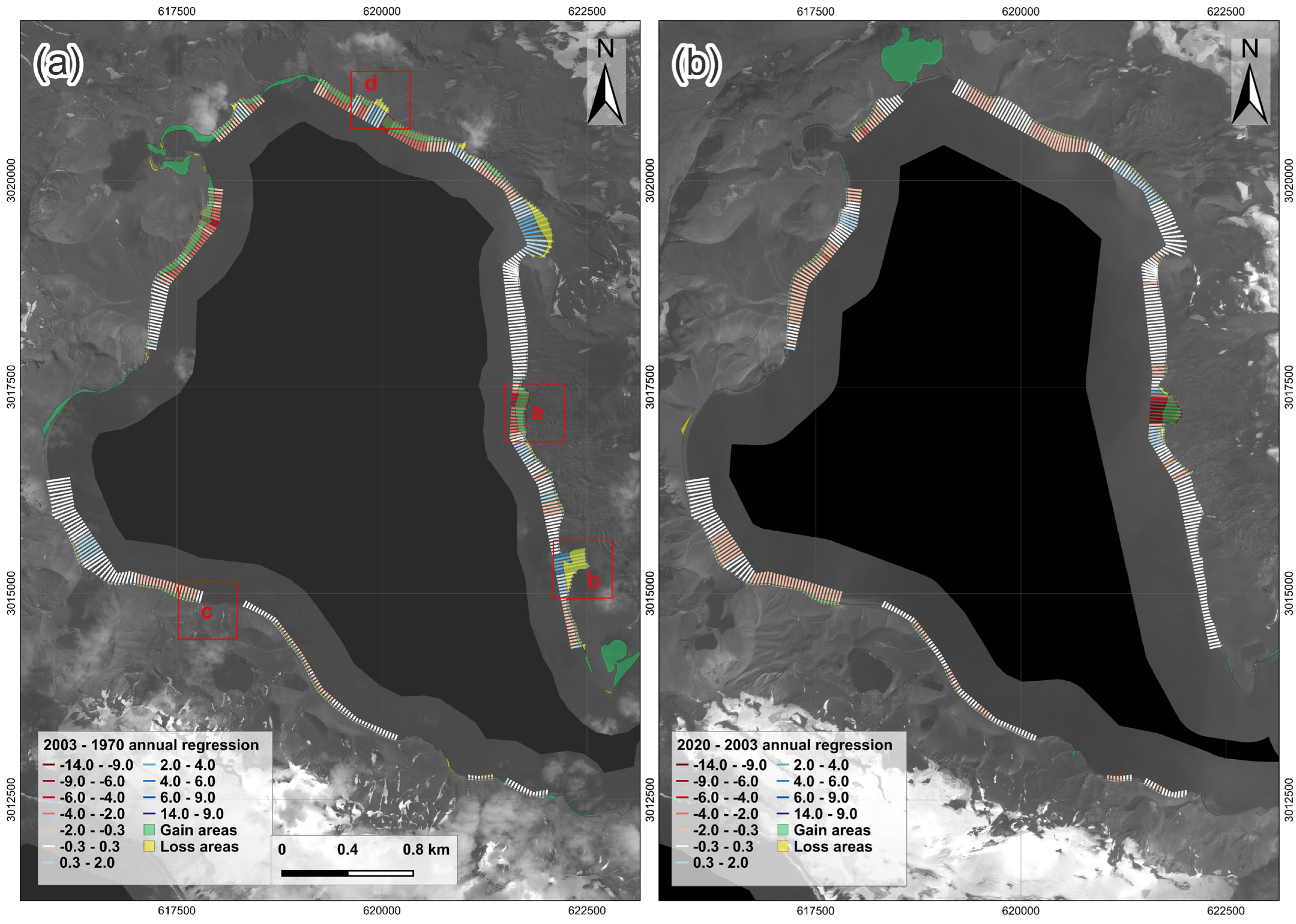
  • Some coastal erosion areas have been detected, consistent with the model dynamics and bathymetric changes (zones 1 and 2). The erosion of this coastline is minimal on the border with the south orientation, but walking paths could be affected. The erosion rates in the areas not affected by the eruption in the first stage studied (southern coastline) are like those found in the second stage on the eroded cliffs along the whole bay, with values of 0.3–2 m/year. The same applies for the sedimentary areas in the two periods studied, to the southwest of Port Foster (west of zone 6) and to the northwest of the bay (north of zone 4), with a sedimentation rate of 0.3–2 m/year. If this model is upheld over time, the evacuation routes along the inner coast and the access to active scientific bases will not be affected.
  • A visual study of the coastline for the periods between 1970 and between 2003 and 2003 and 2020 revealed annual rates of the increase in the water area of the inner bay of 0.023 km2/year and 0.028 km2/year, and annual sedimentation rates of 0.007 km2/year and 0.002 km2/year, respectively. It also revealed a discrepancy in front of scientific bases, where it identified substantial erosion on the slope facing the beach. This dynamic could indeed affect the accessibility of the bases. The evolution of the coastline demonstrates erosional ratios of up to 2 m/year in slopes/cliff.
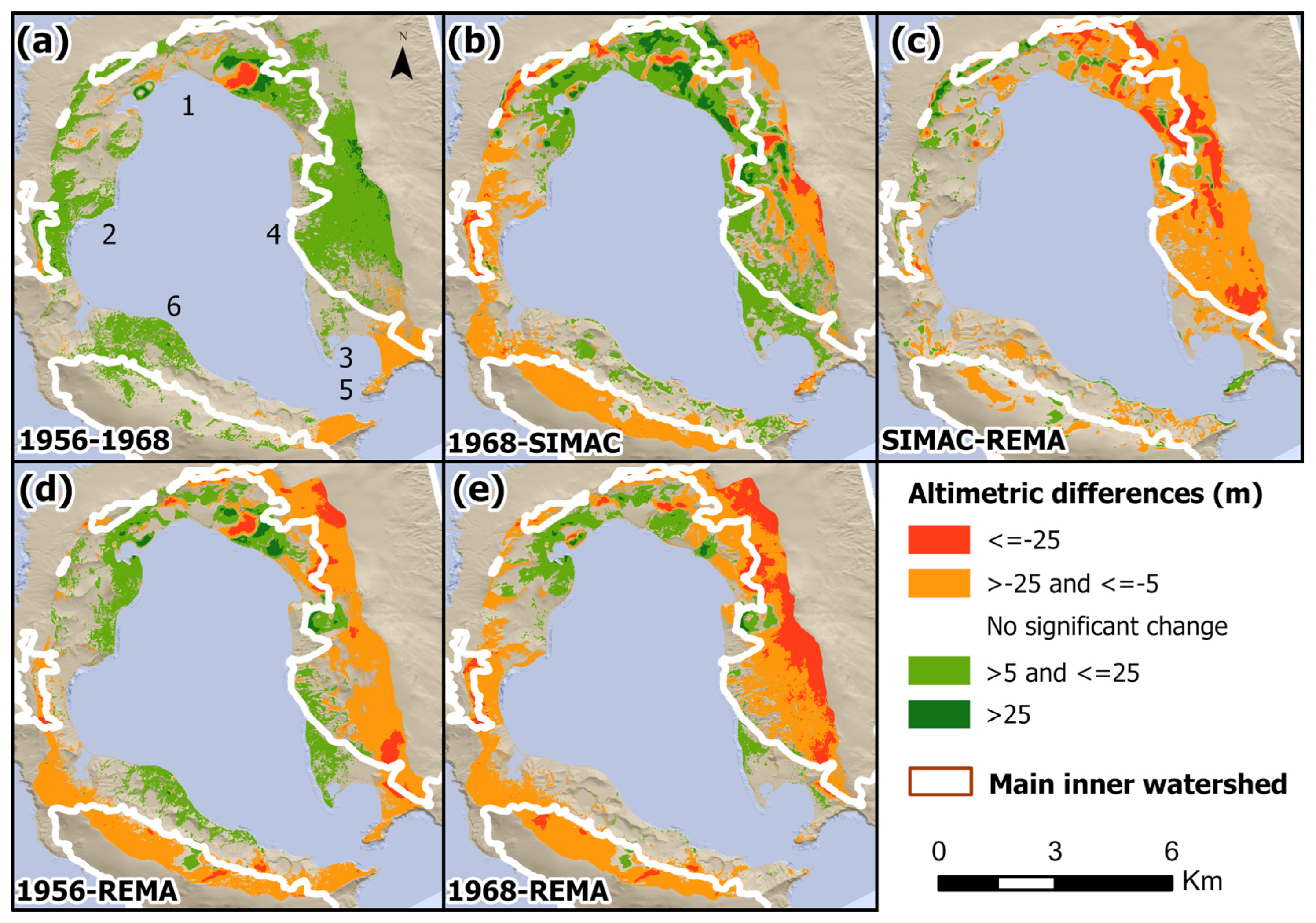
  • While the overall size of the island has been decreasing over time, this reduction is much greater than that observed in the bay because it is linked to possible ice loss in areas above 300 m in elevation. It was challenging to discriminate areas with accumulated snow because many of them are covered with ash and blend in with the ground. Also, in less than 15 years, four craters from the last event became near-invisible, with infill values up to 9 m. A considerable part of the overall loss of surface material is received within the bay, including its own erosion from the submerged caldera’s lateral walls, and accumulates at the bay’s bottom. However, there is a substantial outward transfer of material to balance the figures. These observations highlight the dynamic nature of the coastline and the impact of various factors on the erosion and sedimentation processes on the inner coast.
  • Finally, though it was not the study’s objective, it is essential to highlight the significant retreat experienced by the only glacier of the island, which increased in its annual retreat to 14 m in the 2003–2020 interval compared to the 7 m/year it experienced between 1970 and 2003, representing a 100% increase in its annual retreat. This loss aligns with the DEM volumetric loss detected primarily in the high-altitude area and linked to snow mass loss.
Although the model was focused primarily on other factors such as tidal currents and morphodynamic processes, it could be improved by including changes in air pressure and wind at more points on the island, to introduce both spatial and temporal variation, as well as by conducting an extensive field survey with different locations of tides and currents, to calibrate and validate the model more accurately.
Also, this study used historical data with metres of uncertainty and some field data. While resampling techniques were applied and slope ranges were defined, altimetric/bathymetric differences showed high values, and spatial–temporal trends did not offer statistical significance in all temporal studies. These altimetric differences, along with the bathymetric modification we found, require the acquisition of new precise DEM, maybe with unmanned aerial vehicle (UAV) flight, as well as new bathymetry and snowmelt runoff measurements to improve and validate these results.

Author Contributions

Conceptualisation, C.T. and C.Z.; methodology, C.T., C.Z., J.d.l.F. and G.P.; validation, C.T. and B.J.-A.; formal analysis, C.T., C.Z. and J.d.l.F.; writing—original draft preparation, C.T., C.Z. and J.d.l.F.; writing—review and editing, C.T., C.Z., J.d.l.F., B.J.-A. and G.P.; visualisation, C.T., C.Z., J.d.l.F. and G.P.; supervision, C.T. All authors have read and agreed to the published version of the manuscript.

Funding

This research was funded by the Spanish Ministry of Economy, Industry and Competitiveness project: “Seguimiento y vigilancia de procesos geodinámicos activos mediante deformación geodésica GNSS en diferentes escenarios (Antártida, Golfo de Cádiz y Latinoamérica)” (CTM2017-84210-R), and the Portuguese Science and Technology Foundation through the Portuguese Polar Program under the PERMANTAR projects (PROPOLAR/FCT) and THAWIMPACT/2022.06628.PTDC.

Data Availability Statement

SIMAC information can be request through an email to the corresponding author.

Acknowledgments

Special thanks go to the Hydrographic Institute of the Spanish Navy (In Spanish: Instituto Hidrográfico de la Marina) and promoters of global projects such as the Marine Geoscience Data System (MGDS) or Antarctic projects such as the Reference Elevation Model of Antarctica (REMA). Reviews by five anonymous were much appreciated.

Conflicts of Interest

The authors declare no conflicts of interest. The founding sponsors had no role in the design of this study; in the collection, analyses, or interpretation of data; in the writing of the manuscript; or in the decision to publish the results.

Appendix A

Figure A1. MGDS point data from the Laurence M. Gould expedition. All images have the same projection (EPSG: 32720), scale, and north orientation.
Remotesensing 16 00512 g0a1

Appendix B

Table A1. Characteristics of river discharges of Deception Island according to the numbering in Figure 5.
IDFlow (m3/s)TributaryMain River Length (m)LocationEntity
10.020469.61Argentine Base2
20.042619.7Argentine Base3
30.0251291.25Argentine Base2
40.010123Argentine Base1
50.020640.49West2
60.0453672.63West3
70.030786.49West3
80.020607.32West2
90.08591370.98West4
100.09101452.21West4
110.0881279.49West4
120.020533.19Argentine Base2
130.020400.21West2
140.032234.12Lake2
150.010148.37Lake1
160.01097.95Lake1
170.010103.89Lake1
180.020281.63Lake2
190.032240.08Lake2
200.010185.01Lake1
210.0353311.28Lake2
220.010219.38Lake1
230.020260.81Lake2
240.010143.72Lake1
250.042570.33Lake3
260.07551392.13North5
270.07551515.12North5
280.0553997.16North-East4
290.0555775.87North-East3
300.032391.4Crater_702
310.0653563.25Crater_705
320.010492.86Crater_701
330.032327.24North-West2
340.032855.77Black glacier2
350.0251495.97Black glacier2
360.010440West1
370.010350West1
380.0253370South-West1
390.020997.17Entry2
400.0761626.25Entry4
410.05531622.69Entry4
420.03531247.65Entry2
430.0555577.57Entry3
440.054714.78Entry3
450.0655973.48Entry4
460.06551280.05Entry4
470.010724.61Spanish Base1
480.0861363.3Argentine Base5
490.042820.57Argentine Base3
500.0151456.07Argentine Base1
510.0151336.87Argentine Base1
520.042332.73Entry3
530.064750.3Entry4
540.0959454.17Argentine Base5
550.0541316.89Argentine Base3
Table A2. Ellipsoidal height differences between GPS points and REMA in CR70.
No. of Point2006 h (m)REMA h (m)2006 h–REMA h (m)
152.250.1−2.0
261.159.6−1.5
357.756.4−1.3
443.252.18.9
580.186.46.3
662.956.1−6.8
759.854.4−5.4
890.383.8−6.5
998.187.9−10.2
1094.186.7−7.5
1169.865.7−4.1
1250.450.1−0.3
1365.461.1−4.3
1477.574.9−2.6
1564.562.5−2.0
1657.364.47.1
1781.379.8−1.5
1893.790.4−3.4
1998.495.5−2.9
2034.240.36.1
21108.9105.0−3.9
2245.146.91.9
2345.145.0−0.1
2448.954.05.2
2548.047.2−0.7
2646.744.6−2.1
2746.646.3−0.3

References

  1. McLean, L.; Rock, J. The Importance of Antarctica: Assessing the Values Ascribed to Antarctica by Its Researchers to Aid Effective Climate Change Communication. Polar J. 2016, 6, 291–306. [Google Scholar] [CrossRef]
  2. Rosado, B.; Fernández-Ros, A.; Berrocoso, M.; Prates, G.; Gárate, J.; deGil, A.; Geyer, A. Volcano-Tectonic Dynamics of Deception Island (Antarctica): 27 years of GPS Observations (1991–2018). J. Volcanol. Geotherm. Res. 2019, 381, 57–82. [Google Scholar] [CrossRef]
  3. Jiménez-Morales, V.; Almendros, J.; Carmona, E. Long-Term Evolution of the Seismic Activity Preceding the 2015 Seismic Crisis at Deception Island Volcano, Antarctica (2008–2015). Surv. Geophys. 2022, 43, 959–994. [Google Scholar] [CrossRef]
  4. Pedrazzi, D.; Kereszturi, G.; Lobo, A.; Geyer, A.; Calle, J. Geomorphology of the Post-Caldera Monogenetic Volcanoes at Deception Island, Antarctica—Implications for Landform Recognition and Volcanic Hazard Assessment. J. Volcanol. Geotherm. Res. 2020, 402, 106986. [Google Scholar] [CrossRef]
  5. Geyer, A.; Álvarez-Valero, A.M.; Gisbert, G.; Aulinas, M.; Hernández-Barreña, D.; Lobo, A.; Marti, J. Deciphering the Evolution of Deception Island’s Magmatic System. Sci. Rep. 2019, 9, 373. [Google Scholar] [CrossRef] [PubMed]
  6. Roberts, S.J.; Monien, P.; Foster, L.C.; Loftfield, J.; Hocking, E.P.; Schnetger, B.; Pearson, E.J.; Juggins, S.; Fretwell, P.; Ireland, L.; et al. Past Penguin Colony Responses to Explosive Volcanism on the Antarctic Peninsula. Nat. Commun. 2017, 8, 14914. [Google Scholar] [CrossRef]
  7. Lewis Smith, R.I. The Bryophyte Flora of Geothermal Habitats on Deception Island, Antarctica. J. Hattori Bot. Lab. 2005, 97, 233–248. [Google Scholar] [CrossRef]
  8. Smith, K.L. (Ed.) Ecosystem Studies at Deception Island, Antarctica; Elsevier: Amsterdam, The Netherlands, 2003; Volume 50. [Google Scholar]
  9. Dibbern, J.S. Fur Seals, Whales and Tourists: A Commercial History of Deception Island, Antarctica. Polar Rec. 2010, 46, 210–221. [Google Scholar] [CrossRef]
  10. Secretariat of the Antarctic Treaty. Compilation of Key Documents of the Antarctic Treaty System, 2nd ed.; Secretariat of the Antarctic Treaty: Bueno Aires, Argentina, 2014; ISBN 978-987-1515-76-9. [Google Scholar]
  11. Torrecillas, C.; Berrocoso, M. The Multidisciplinary Scientific Information Support System (SIMAC) for Deception Island. In Antarctica; Springer: Berlin/Heidelberg, Germany, 2006; pp. 397–402. [Google Scholar] [CrossRef]
  12. Bartolini, S.; Geyer, A.; Martí, J.; Pedrazzi, D.; Aguirre-Díaz, G. Volcanic Hazard on Deception Island (South Shetland Islands, Antarctica). J. Volcanol. Geotherm. Res. 2014, 285, 150–168. [Google Scholar] [CrossRef]
  13. Smellie, J.L. Lithostratigraphy and Volcanic Evolution of Deception Island, South Shetland Islands. Antarct. Sci. 2001, 13, 188–209. [Google Scholar] [CrossRef]
  14. Clapperton, C.M. The Volcanic Eruption At Deception Island, December 1967. Br. Antarct. Surv. Bull. 1969, 22, 83–90. [Google Scholar]
  15. Smellie, J.L. The 1969 Subglacial Eruption on Deception Island (Antarctica): Events and Processes during an Eruption beneath a Thin Glacier and Implications for Volcanic Hazards. J. Volcanol. Geotherm. Res. 2002, 80, 17–25. [Google Scholar] [CrossRef]
  16. Aristarain, A.J.; Delmas, R.J. Ice Record of a Large Eruption of Deception Island Volcano (Antarctica) in the XVIIth Century. J. Volcanol. Geotherm. Res. 1998, 80, 17–25. [Google Scholar] [CrossRef]
  17. Birkenmajer, K. Lichenometric Dating of a Mid-19th Century Lava Eruption on Deception Island (West Antarctica). Bull. Pol. Acad. Sci. Earth Sci. 1991, 39, 467–475. [Google Scholar]
  18. DeConto, R.M.; Pollard, D. Contribution of Antarctica to Past and Future Sea-Level Rise. Nature 2016, 531, 591–597. [Google Scholar] [CrossRef] [PubMed]
  19. Almar, R.; Ranasinghe, R.; Bergsma, E.W.J.; Diaz, H.; Melet, A.; Papa, F.; Vousdoukas, M.; Athanasiou, P.; Dada, O.; Almeida, L.P.; et al. A Global Analysis of Extreme Coastal Water Levels with Implications for Potential Coastal Overtopping. Nat. Commun. 2021, 12, 3775. [Google Scholar] [CrossRef]
  20. Vousdoukas, M.I.; Mentaschi, L.; Voukouvalas, E.; Verlaan, M.; Jevrejeva, S.; Jackson, L.P.; Feyen, L. Global Probabilistic Projections of Extreme Sea Levels Show Intensification of Coastal Flood Hazard. Nat. Commun. 2018, 9, 2360. [Google Scholar] [CrossRef] [PubMed]
  21. Turner, J.; Barrand, N.E.; Bracegirdle, T.J.; Convey, P.; Hodgson, D.A.; Jarvis, M.; Jenkins, A.; Marshall, G.; Meredith, M.P.; Roscoe, H.; et al. Antarctic Climate Change and the Environment: An Update. Polar Rec. 2014, 50, 237–259. [Google Scholar] [CrossRef]
  22. Prates, G.; Vieira, G. Surface Displacement of Hurd Rock Glacier from 1956 to 2019 from Historical Aerial Frames and Satellite Imagery (Livingston Island, Antarctic Peninsula). Remote Sens. 2023, 15, 3685. [Google Scholar] [CrossRef]
  23. Prates, G.; Torrecillas, C.; Berrocoso, M.; Goyanes, G.; Vieira, G. Deception Island 1967–1970 Volcano Eruptions from Historical Aerial Frames and Satellite Imagery (Antarctic Peninsula). Remote Sens. 2023, 15, 2052. [Google Scholar] [CrossRef]
  24. Lesser, G.R.; Roelvink, J.A.; van Kester, J.A.T.M.; Stelling, G.S. Development and Validation of a Three-Dimensional Morphological Model. Coast. Eng. 2004, 51, 883–915. [Google Scholar] [CrossRef]
  25. Iglesias, G.; Sánchez, M.; Carballo, R.; Fernández, H. The TSE Index—A New Tool for Selecting Tidal Stream Sites in Depth-Limited Regions. Renew. Energy 2012, 48, 350–357. [Google Scholar] [CrossRef]
  26. Hansen, J.E.; Elias, E.; List, J.H.; Erikson, L.H.; Barnard, P.L. Tidally Influenced Alongshore Circulation at an Inlet-Adjacent Shoreline. Cont. Shelf Res. 2013, 56, 26–38. [Google Scholar] [CrossRef]
  27. Ruggiero, P.; Walstra, D.J.R.; Gelfenbaum, G.; van Ormondt, M. Seasonal-Scale Nearshore Morphological Evolution: Field Observations and Numerical Modeling. Coast. Eng. 2009, 56, 1153–1172. [Google Scholar] [CrossRef]
  28. Van Rijn, L.C. Unified View of Sediment Transport by Currents and Waves. I: Initiation of Motion, Bed Roughness, and Bed-Load Transport. J. Hydraul. Eng. 2007, 133, 649–667. [Google Scholar] [CrossRef]
  29. Roobol, M.J. A Model for the Eruptive Mechanism of Deception Island from 1820 to 1970. Br. Antarct. Surv. Bull. 1980, 49, 137–156. [Google Scholar]
  30. Baker, P.E.; Roobol, M.J.A.; Davies, S.M.; McReath, I.; Harvey, M.R. The Geology of the South Shetland Islands: V. Volcanic Evolution of Deception Island. Br. Antarct. Surv. Sci. Rep. 1975, 78, 79. [Google Scholar]
  31. Ortiz, R.; Vila, J.; Garcia, A.; Camacho, A.G.; Diez, J.L.; Aparicio, A.; Soto, R.; Viramonte, J.G.; Risso, C.; Petrinovic, I.; et al. Geophysical Features of Deception Island. In Recent Progress in Antarctic Earth Science; Yoshida, Y., Ed.; Terrapub: Tokyo, Japan, 1992; pp. 443–448. [Google Scholar]
  32. Torrecillas, C.; Berrocoso, M.; Pérez-López, R.; Torrecillas, M.D. Determination of Volumetric Variations and Coastal Changes Due to Historical Volcanic Eruptions Using Historical Maps and Remote-Sensing at Deception Island (West-Antarctica). Geomorphology 2012, 136, 6–14. [Google Scholar] [CrossRef]
  33. Cooper, A.P.R.; Smellie, J.L.; Maylin, J. Evidence for Shallowing and Uplift from Bathymetric Records of Deception Island, Antarctica. Antarct. Sci. 1998, 10, 455–461. [Google Scholar] [CrossRef]
  34. Berrocoso, M.; Torrecillas, C.; Jigena, B.; Fernández-Ros, A. Determination of Geomorphological and Volumetric Variations in the 1970 Land Volcanic Craters Area (Deception Island, Antarctica) from 1968 Using Historical and Current Maps, Remote Sensing and GNSS. Antarct. Sci. 2012, 24, 367–376. [Google Scholar] [CrossRef]
  35. Hans Nelson, C.; Bacon, C.R.; Robinson, S.W.; Adam, D.P.; Platt Bradbury, J.; Barber, J.H.; Schwartz, D.; Vagenas, G. The Volcanic, Sedimentologic, and Paleolimnologic History of the Crater Lake Caldera Floor, Oregon: Evidence for Small Caldera Evolution. Geol. Soc. Am. Bull. 1994, 106, 684–704. [Google Scholar] [CrossRef]
  36. Roobol, M.J. Historic Vulcanic Activity at Deception Island. Br. Antarct. Surv. Bull. 1973, 32, 23–30. [Google Scholar]
  37. Flexas, M.M.; Arias, M.R.; Ojeda, M.A. Hydrography and Dynamics of Port Foster, Deception Island, Antarctica. Antarct. Sci. 2017, 29, 83–93. [Google Scholar] [CrossRef]
  38. Jigena Antelo, B.; Vidal, J.; Berrocoso, M. Determination of the Tide Constituents at Livingston and Deception Islands (South Shetland Islands, Antarctica), Using Annual Time Series. Dyna 2015, 82, 209–218. [Google Scholar] [CrossRef]
  39. Jigena, B.; Vidal, J.; Berrocoso, M. Determination of the Mean Sea Level at Deception and Livingston Islands, Antarctica. Antarct. Sci. 2014, 27, 101–102. [Google Scholar] [CrossRef]
  40. Berrocoso, M.; Prates, G.; Fernández-Ros, A.; Peci, L.M.; de Gil, A.; Rosado, B.; Páez, R.; Jigena, B. Caldera Unrest Detected with Seawater Temperature Anomalies at Deception Island, Antarctic Peninsula. Bull. Volcanol. 2018, 80, 41. [Google Scholar] [CrossRef]
  41. Martins Figueiredo, D. Hydrodynamic Modelling of Port Foster (Deception Island, Antarctica) Implementation of a Two-Dimensional Tidal Model and an Approach on the Three-Dimensional Model as Well as Generation of Internal Waves; Engenharia Do Ambiente: Lisboa, Portugal, 2015; Available online: https://fenix.tecnico.ulisboa.pt/downloadFile/1126295043834448/ExtendedAbstract_DanielFigueiredo.pdf (accessed on 24 January 2024).
  42. Figueiredo, D.; Dos Santos, A.; Mateus, M.; Pinto, L. Hydrodynamic Modelling of Port Foster, Deception Island, Antarctica. Antarct. Sci. 2018, 30, 115–124. [Google Scholar] [CrossRef]
  43. Smellie, J.L.; López-Martínez, J.; Headland, R.K.; Hernández-Cifuentes, F.; Maestro, A.; Millar, I.L.; Rey, J.; Serrano, E.; Somoza, L.; Thomson, J.W. Geology and Geomorphology of Deception Island; López-Martínez, J., Smellie, J.L., Thomson, J.W., Thomson, M.R.A., Eds.; British Antarctic Survey: Cambridge, UK, 2002. [Google Scholar]
  44. Servicio Geográfico del Ejercito. Universidad Autónoma de Madrid. Deception Island Map 1:25,000. Spanish Antarctic Cartography; Servicio Geográfico del Ejercito: Madrid, Spain, 1994. [Google Scholar]
  45. Centro Geográfico del Ejército español. New Topographic Map of Deception Island 1:25,000; Centro Geográfico del Ejército español: Madrid, Spain, 2006. [Google Scholar]
  46. Berrocoso, M.; Fernández-Ros, A.; Torrecillas, C.; Enríquez de Salamanca, J.M.; Ramírez, M.E.; Pérez-Peña, A.; González, M.J.; Páez, R.; Jiménez, Y.; García-García, A.; et al. Geodetic Research on Deception Island. In Antarctica; Springer: Berlin/Heidelberg, Germany, 2006; pp. 391–396. [Google Scholar]
  47. Howat, I.M.; Porter, C.; Smith, B.E.; Noh, M.J.; Morin, P. The Reference Elevation Model of Antarctica. Cryosphere 2019, 13, 665–674. [Google Scholar] [CrossRef]
  48. Brecher, H.H. Institute of Polar Studies Photogrammetric Maps of a Volcanic Eruption Area, Deception Island, Antarctica; Research Foundation and the Institute of Polar Studies, The Ohio State University: Columbus, OH, USA, 1975. [Google Scholar]
  49. Directorate of Overseas Survey (D.O.S.). Deception Island Map 1:25,000; Ordnance Survey: Southampton, UK, 1959. [Google Scholar]
  50. Jigena, B.; Berrocoso, M.; Torrecillas, C.; Vidal, J.; Barbero, I.; Fernandez-Ros, A. Determination of an Experimental Geoid at Deception Island, South Shetland Islands, Antarctica. Antarct. Sci. 2016, 28, 277–292. [Google Scholar] [CrossRef]
  51. Braun, A. Retrieval of Digital Elevation Models from Sentinel-1 Radar Data—Open Applications, Techniques, and Limitations. Open Geosci. 2021, 13, 532–569. [Google Scholar] [CrossRef]
  52. Somoza, L.; Martínez-Frías, J.; Smellie, J.; Rey, J.; Maestro, A. Evidence for hydrothermal venting and sediment volcanism discharged after recent short-lived volcanic eruptions at Deception Island, Bransfield Strait, Antarctica. Mar. Geol. 2004, 203, 119–140. [Google Scholar] [CrossRef]
  53. Rey, J.; Maestro, A.; Somoza, L.; Smellie, J.L. Submarine Morphology and Seismic Stratigraphy of Port Foster. In Geology and Geomorphology of Deception Island; López-Martínez, J., Smellie, J.L., Thomson, J.W., Thomson, M.R.A., Eds.; British Antarctic Survey: Cambridge, UK, 2002; pp. 40–46. [Google Scholar]
  54. Hopfenblatt, J.; Geyer, A.; Aulinas, M.; Álvarez-Valero, A.M.; Gisbert, G.; Kereszturi, G.; Ercilla, G.; Gómez-Ballesteros, M.; Márquez, A.; García-Castellanos, D.; et al. Formation of Stanley Patch Volcanic Cone: New Insights into the Evolution of Deception Island Caldera (Antarctica). J. Volcanol. Geotherm. Res. 2021, 415, 107249. [Google Scholar] [CrossRef]
  55. Barclay, A.H.; Wilcock, W.S.D.; Ibanez, J.M.; Ibáñez, J.M. Bathymetric Constraints on the Tectonic and Volcanic Evolution of Deception Island Volcano, South Shetland Islands. Antarct. Sci. 2009, 21, 153–167. [Google Scholar] [CrossRef]
  56. Smith, K.L. Underway Hydrographic, Weather and Ship-State Data (JGOFS) from Laurence M. Gould Expedition LMG0010 (2000); Interdisciplinary Earth Data Alliance (IEDA): New York, NY, USA, 2014. [Google Scholar]
  57. Smith, C. Underway Hydrographic, Weather and Ship-State Data (JGOFS) from Laurence M. Gould Expedition LMG0102 (2001); Interdisciplinary Earth Data Alliance (IEDA): New York, NY, USA, 2012. [Google Scholar]
  58. Blanchette, R. Underway Hydrographic, Weather and Ship-State Data (JGOFS) from Laurence M. Gould Expedition LMG0704 (2007); Interdisciplinary Earth Data Alliance (IEDA): New York, NY, USA, 2010. [Google Scholar]
  59. Leger, D. Underway Hydrographic, Weather and Ship-State Data (JGOFS) from Laurence M. Gould Expedition LMG0712 (2007); Interdisciplinary Earth Data Alliance (IEDA): New York, NY, USA, 2009. [Google Scholar]
  60. Blanchette, R. Underway Hydrographic, Weather and Ship-State Data (JGOFS) from Laurence M. Gould Expedition LMG0903 (2009); Interdisciplinary Earth Data Alliance (IEDA): New York, NY, USA, 2011. [Google Scholar]
  61. Fremand, A.C. A Bathymetric Compilation of the South Shetland Islands, 1991–2017; British Antarctic Survey: Cambridge, UK, 2019. [Google Scholar]
  62. Van Rijn, L.C. Principles of Sediment Transport in Rivers, Estuaries and Coastal Seas; Aqua Publications: Blokzijl, The Netherlends, 1993. [Google Scholar]
  63. QGIS.org QGIS Geographic Information System. Open Source Geospatial Foundation Project. 2024. Available online: https://qgis.org/ (accessed on 24 January 2024).
  64. Environmental Systems Research Institute, Inc. R.C. ArcGIS Pro. Version 3.1. 2010. Available online: www.arcgis.com (accessed on 28 September 2023).
  65. Tanguy, R.; Whalen, D.; Prates, G.; Vieira, G. Shoreline Change Rates and Land to Sea Sediment and Soil Organic Carbon Transfer in Eastern Parry Peninsula from 1965 to 2020 (Amundsen Gulf, Canada). Arct. Sci. 2023, 9, 506–525. [Google Scholar] [CrossRef]
  66. Molina, R.; Anfuso, G.; Manno, G.; Prieto, F.J.G. The Mediterranean Coast of Andalusia (Spain): Medium-Term Evolution and Impacts of Coastal Structures. Sustainability 2019, 11, 3539. [Google Scholar] [CrossRef]
  67. Lenn, Y.-D.; Chereskin, T.K.; Glatts, R.C. Seasonal to Tidal Variability in Currents, Stratification and Acoustic Backscatter in an Antarctic Ecosystem at Deception Island. Deep. Sea Res. Part II Top. Stud. Oceanogr. 2003, 50, 1665–1683. [Google Scholar] [CrossRef]
  68. Vidal, J.; Berrocoso, M.; Jigena, B. Hydrodynamic Modeling of Port Foster, Deception Island (Antarctica). In Nonlinear and Complex. Dynamics; Springer: New York, NY, USA, 2011; pp. 193–203. [Google Scholar] [CrossRef]
  69. Parker, B.B.; Gutierrez, C.M.; Lautenbacher, C.C.; Dunnigan, J.H.; Administrator, A.; Szabados, M. Tidal Analysis and Prediction Center for Operational Oceanographic Products and Services; NOAA, NOS Center for Operational Oceanographic Products and Services: Silver Spring, MD, USA, 2007. [Google Scholar]
  70. Eelkema, M.; Wang, Z.B.; Stive, M.J.F. Impact of Back-Barrier Dams on the Development of the Ebb-Tidal Delta of the Eastern Scheldt. J. Coast. Res. 2012, 285, 1591–1605. [Google Scholar] [CrossRef]
  71. Dissanayake, P.; Wurpts, A. Modelling an Anthropogenic Effect of a Tidal Basin Evolution Applying Tidal and Wave Boundary Forcings: Ley Bay, East Frisian Wadden Sea. Coast. Eng. 2013, 82, 9–24. [Google Scholar] [CrossRef]
  72. Luijendijk, A.P.; Ranasinghe, R.; de Schipper, M.A.; Huisman, B.A.; Swinkels, C.M.; Walstra, D.J.R.; Stive, M.J.F. The Initial Morphological Response of the Sand Engine: A Process-Based Modelling Study. Coast. Eng. 2017, 119, 1–14. [Google Scholar] [CrossRef]
  73. Zarzuelo, C.; López-Ruiz, A.; Ortega-Sánchez, M. Evaluating the Impact of Dredging Strategies at Tidal Inlets: Performance Assessment. Sci. Total Environ. 2019, 658, 1069–1084. [Google Scholar] [CrossRef]
  74. Nienhuis, J.H.; Ashton, A.D.; Nardin, W.; Fagherazzi, S.; Giosan, L. Alongshore Sediment Bypassing as a Control on River Mouth Morphodynamics. J. Geophys. Res. Earth Surf. 2016, 121, 664–683. [Google Scholar] [CrossRef]
  75. Ghilani, C.D.; Wolf, P. Elementary Surveying, Global Edition; Pearson Education Limited: London, UK, 2016; ISBN 9781292060675. [Google Scholar]
  76. Pattyn, F.; Ritz, C.; Hanna, E.; Asay-Davis, X.; DeConto, R.; Durand, G.; Favier, L.; Fettweis, X.; Goelzer, H.; Golledge, N.R.; et al. The Greenland and Antarctic Ice Sheets under 1.5 °C Global Warming. Nat. Clim. Chang. 2018, 8, 1053–1061. [Google Scholar] [CrossRef]
  77. Roobol, M.J. The Volcanic Hazard at Deception Island, South Shetland Islands. Br. Antarct. Surv. Bull. 1982, 51, 237–245. [Google Scholar]
Figure 2. Some 1968–2003–2020 [23] visual geomorphological changes at Deception Island in four areas (zones a, b, c, and d linked to red squares in Figure 1b). First row, the early situation, and below, a later date showing the change. In particular: (a1, a2) shows seven new volcanoes of the 1970 eruption craters with its inferred rim in orange and its infill; (b1, b2) shows coastal erosion near Kroner Lake and opening to Port Foster using a new 1968 orthophoto in (b1) and an overlap of the 1968 coastline (purple line); (c1, c2) shows coastal erosion near “Lago Escondido” and its opening to Port Foster with the 1968 coastline (purple line) in (c1) and 2003 coastline (red line) in (c2); and (d1, d2) shows Black Glacier retreat acceleration with the same coastlines as in column c. All images have the same projection (EPSG: 32720), scale, and north orientation.
Remotesensing 16 00512 g002
Figure 3. General methodology.
Remotesensing 16 00512 g003
Figure 4. Details of the GIS processes involved in “Historical rates” and “Temporal changes and Altimetric differences” from the general methodology shown in Figure 3.
Remotesensing 16 00512 g004
Figure 5. Mesh composition with COLA station (green diamond), tidal boundary, and melting streams with their tributaries and discharge points (EPSG: 32720).
Remotesensing 16 00512 g005
Figure 6. Calibration for COLA station. Blue circles correspond to the measured tide level data, and the white filled circles to the computed tide level data.
Remotesensing 16 00512 g006
Figure 7. Results of the sensitivity study on the currents, changing the Chèzy coefficient at 45, 60, and 100.
Remotesensing 16 00512 g007
Figure 8. Water depth variation represented as sedimentation (green, negative values) and erosion (red, positive values) after a one-year simulation with the DELFT 3D numerical model and definition of studied zones (EPSG: 32720).
Remotesensing 16 00512 g008
Figure 9. Overlapping annual shoreline regression of gain–loss areas in two different time periods: (a) 1970–2003 with new QB as the background and some enlarged in areas in Figure 10 (red rectangles with letters a, b, c, and d); and (b) 2003–2020 with K3 as the background [23]. Both figures are in EPSG: 32720 and have the same scale and north orientation.
Remotesensing 16 00512 g009
Figure 10. Some 1968 (purple line), 2003 (light green line), and 2020 (blue line) [23] visual coastline changes at Deception Island. Zones a, b, c, and d are linked to the red squares in Figure 9: (a1a3) shows the Black Glacier retreat; (b1b3) shows the sedimentation to the south of the Black Glacier; (c1c3) shows erosion of the existing slope in front of the Spanish base; and column (d1d3) shows erosion in Pendulum Cove. All figures are displayed with the same scale and north orientation in EPSG 32720.
Remotesensing 16 00512 g010
Figure 11. Temporal differences in DEMs over REMA hillshade and permanent snow (white line): (a) 1956–1968 with the studies zones, (b) 1968-SIMAC, (c) SIMAC-REMA, (d) 1956-REMA, and (e) 1968-REMA. All images have the same projection (EPSG: 32720), scale, and north orientation.
Remotesensing 16 00512 g011
Figure 12. (a) Altimetric trend for 1956–2020 (mainly red square with numbers 1, 2 and 3) and inner watersheds; (b) slope ranges from SIMAC DEM; (c) satellite plume areas (own source) and some geomorphological elements from [43]; and (d) altimetric differences in GNSS points for SIMAC-REMA over REMA hillshade. All images have the same projection (EPSG: 32720) and north orientation. (ac) share the same scale.
Remotesensing 16 00512 g012
Figure 13. Statistical data of the differences in the inner basin between the DEMs in rows (ae) and the DBMs in rows (fh). Maximum and minimum values are represented as dashed black lines, standard deviation as a box (light grey for DEM and light blue for DBM), mean values as an orange line, and median values as a red line.
Remotesensing 16 00512 g013
Figure 14. Port Foster temporal DBM study: (a) bathymetric differences between SIMAC and MGDS mean (1991–2005), (b) MGDS mean and IHM (2005–2012), and (c) SIMAC and IHM (1991–2012) including the studied zones 1–7; (d) slope areas in degrees with bathymetry contours of −160 and −150 m from SIMAC DBM (dark blue) and IHM DBM (light blue); (e) heat maps of nos. of points in 50 m cells from all MDGS data; and (f) trend of this MDGS dataset throughout its period (2000–2009). All images have the same projection (EPSG: 32720), scale, and north orientation.
Remotesensing 16 00512 g014
Table 1. Orthophotos, satellite images, coastlines, and cartographic information.
DenominationDigital SourceDescription/
Spatial Resolution or Scale
Acquisition Date
1968 orthophotoOwn from [23]Orthophoto from
SHNA flight/0.8 m
January 1968
2003 New QB 1Own from [11]QuickBird Satellite image/0.6 m20 January 2003
2020 K3 1Own from [23]KOMPSAT-3 2 Satellite image/0.7 m19 February 2020
Sentinel imagesESASentinel 2 Satellite
Images/10 m
30 March 2017
23 February 2019
30 December 2019
8 February 2020
27 December 2020
13 January 2021
6 January 2021
2 February 2021
29 March 2022 (snow cover)
Google Earth imagesGoogle EarthSatellite images/
several resolutions
31 December 1985
1 January 1999
15 January 2002
3 November 2003
20 October 2005 (snow cover)
7 January 2010
29 December 2013
Sediment plumesOwn from all satellite images Visual delineation of sediment plumes2002–2022
Level contoursSIMAC from CGE mapLine/1:25,0001970 and 2003
Melt streamsSIMAC from CGE mapLine/1:25,0001970 and 2003
1968 coastlineOwn from [23]Line/1:25,000January 1968
1970 coastlineSIMAC from [48]Line/1:25,000August 1970
2003 coastlineSIMAC from new QBLine/1:25,00020 January 2003
2020 coastlineOwn from [23]Line/1:25,0009 February 2020
Geomorphological mapSIMAC from [43] Group layers/
1:25,000
2002
1 Generation of a new True-Ortho with REMA. 2 Includes material ©KARI 2020, Distribution (SI Imaging Services, Republic of Korea), all rights reserved.
Table 2. Digital elevation models (DEMs) used with denomination, digital source, file format and its spatial resolution, acquisition date, and altimetric error (σz).
DenominationDigital SourceFormat Used/
Spatial Resolution (m)
Acquisition Dateσz
(m)
DOS DEMSIMAC from [49]ESRI Grid/20 195630
1956 DEM Own from [23]Tiff file/2.7 19564 (20 m in snow areas)
1968 DEM Own from [23]Tiff file/2.7 19684 (20 m in snow areas)
SIMAC DEMSIMAC from CGE mapESRI Grid/2 1968–19863
REMAREMA [47]Two Tiff files (45_04_2_2_2m_v2.0 and 45_05_2_1_2m_v2.0)/2 2009–2021 11
1 Ellipsoidal height.
Table 3. Digital bathymetry models (DBMs) used with denomination, digital source, file format and its spatial resolution, acquisition date, and altimetric error (σz).
DenominationDigital SourceFormat Used/Spatial Resolution or Distance between PointsAcquisition
Date
σz
(m)
SIMAC DBM Adapted from CGE/IHM/IEO [43]ESRI Grid/2 m1988–19914
Bathymetry LMG0010MGDS [56]Ten Dat files/points in line each <120 m20005
Bathymetry LMG0102MGDS [57]One Dat file/points in line each <120 m20015
Bathymetry LMG0704MGDS [58]Two Dat files/points in line each <120 m20075
Bathymetry LMG0712MGDS [59]One Dat file/points in line each <120 m20075
Bathymetry LMG0903MGDS [60]Four Dat files/points in line each <120 m20095
MGDS mean DBMInterpolated from earlier MGDSEsri Grid/50 m2005 15
IHM DBMIHM [37]Esri Grid/10 m2012 (central bay)
2016 (some coastal zones)
0.5
External South Shetlands DBMBritish Antarctic Survey
[61]
A Ascii file/100 m1991–2017unknown
1 Considered as mean time.
Table 4. Amplitude (u) and phase (φ) results of the measured and computed current data of the harmonic components M2 and K1.
u (m/s)φ (°)
MeasuredComputedMeasuredComputed
M20.130.0133334
K10.090.009173180
Table 5. Volumetric study. The 3D area and volume land/water (km3) columns reference each dataset individually. The differences volume between DEMs/DBMs (km3) and ratio (hm3/year) shows the values between the DEM/DBM in the row and the following temporal DEM/DBM.
TypeDatasetPlane (m)ReferenceArea 3D (km2)Vol. Land/
Water
(km3)
Dif. Vol. (km3)Ratio
(hm3/Year)
DEMREMA
(2009–2021)
0ABOVE48.065.94−0.32−0.23
100ABOVE23.932.77−0.23−0.33
200ABOVE12.331.15−0.13−0.37
300ABOVE5.270.37−0.06−0.36
400ABOVE1.480.07−0.02−0.50
SIMAC DEM (1968–1986)0ABOVE48.026.26−0.03−0.03
100ABOVE24.313.00−0.10−0.23
200ABOVE13.251.28−0.09−0.40
300ABOVE5.710.42−0.06−0.60
400ABOVE1.750.09−0.03−0.89
1968 DEM0ABOVE47.426.280.19 0.36
100ABOVE25.503.100.130.46
200ABOVE14.191.370.090.55
300ABOVE6.460.480.060.78
400ABOVE2.120.120.031.38
1956 DEM 0ABOVE47.176.10NA
100ABOVE24.332.97NA
200ABOVE13.511.29NA
300ABOVE6.060.43NA
400ABOVE1.840.09NA
DBMIHM 1 DBM
(2012–2016)
0BELOW38.533.900.090.0966
−100BELOW22.720.830.020.0004
−150BELOW9.320.07−0.02−0.0010
SIMAC 1 DBM (1988–1991)0BELOW37.763.81NA
−100BELOW20.810.81NA
−150BELOW8.600.09NA
1 Resampled to 50 m.
Disclaimer/Publisher’s Note: The statements, opinions and data contained in all publications are solely those of the individual author(s) and contributor(s) and not of MDPI and/or the editor(s). MDPI and/or the editor(s) disclaim responsibility for any injury to people or property resulting from any ideas, methods, instructions or products referred to in the content.

