Evaluation of a LIDAR Land-Based Mobile Mapping System for Monitoring Sandy Coasts

Abstract
:
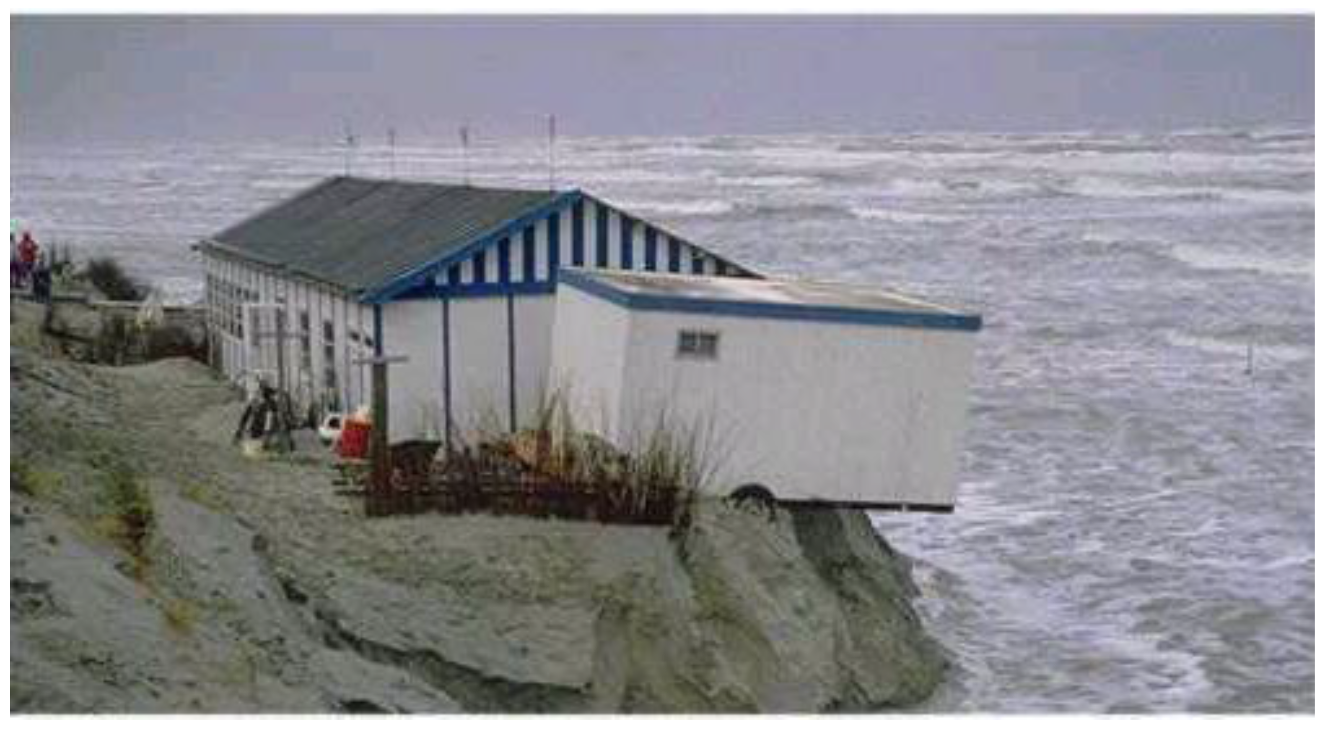
1. Introduction

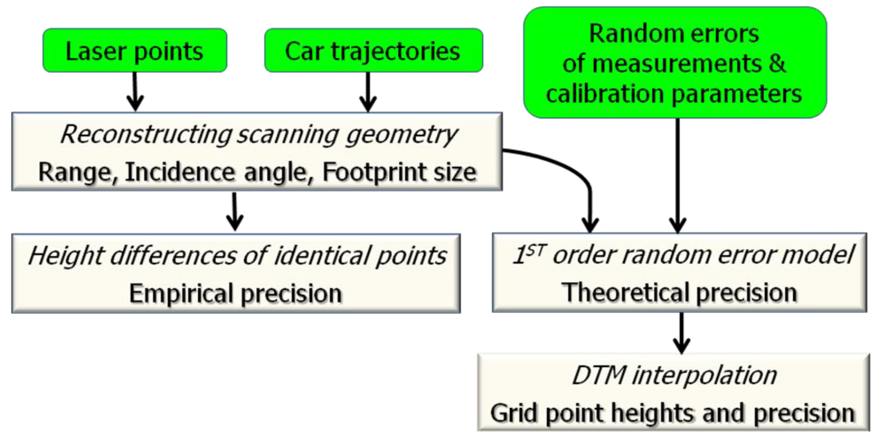
2. An Overview of Processing Steps

3. Quality of Laser Point Heights
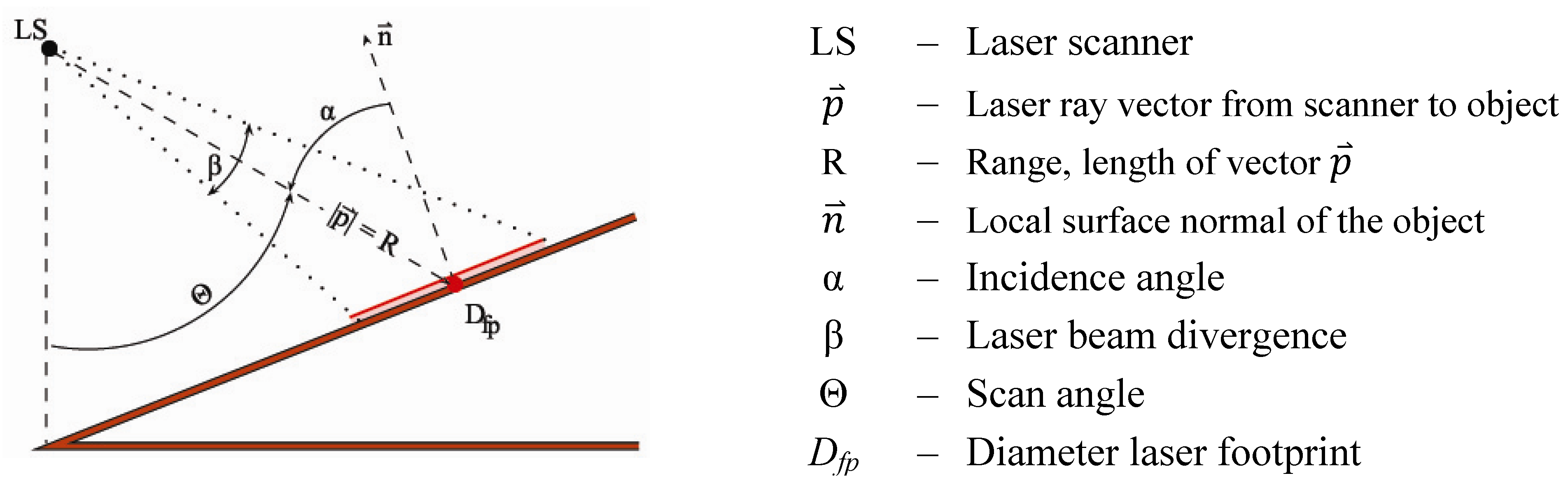
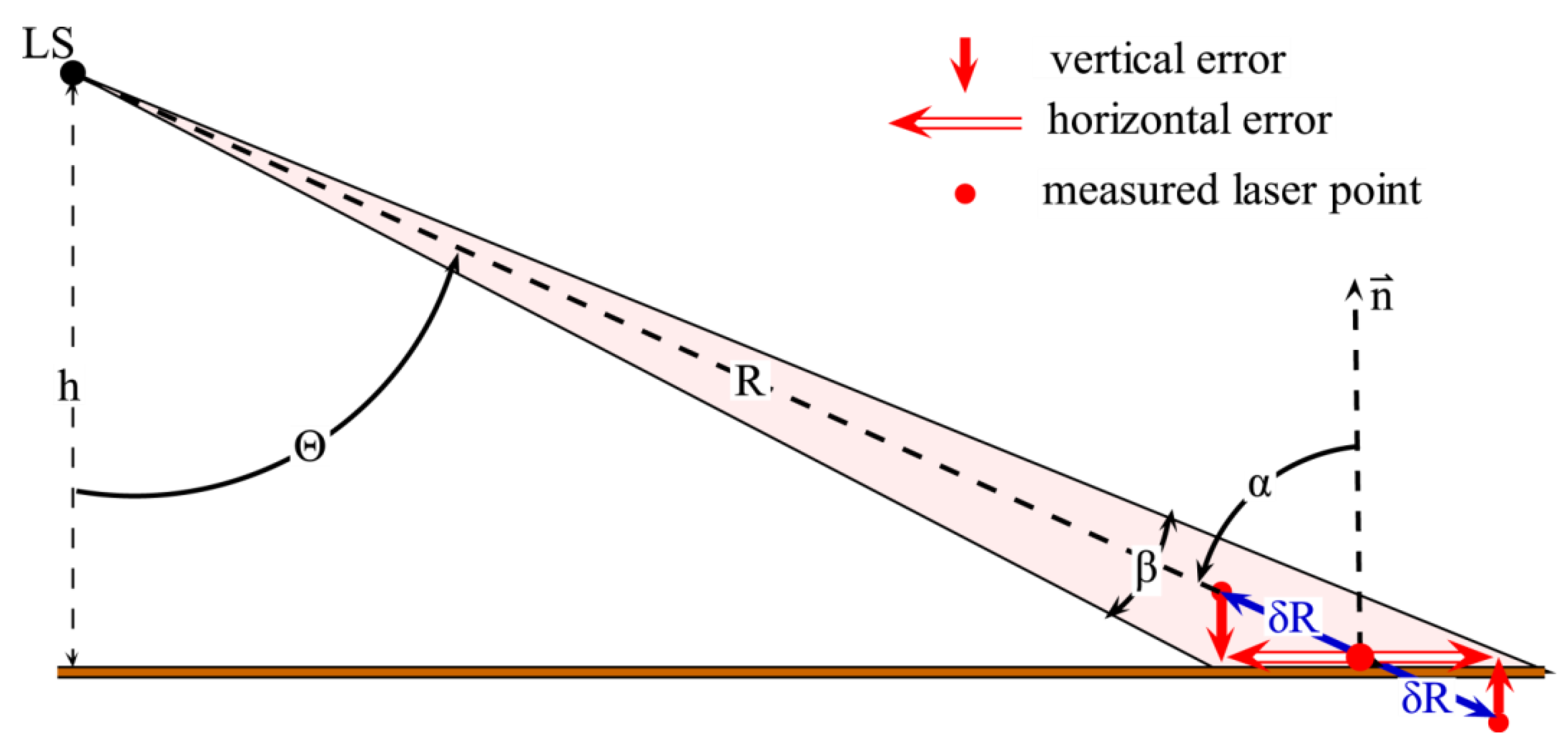
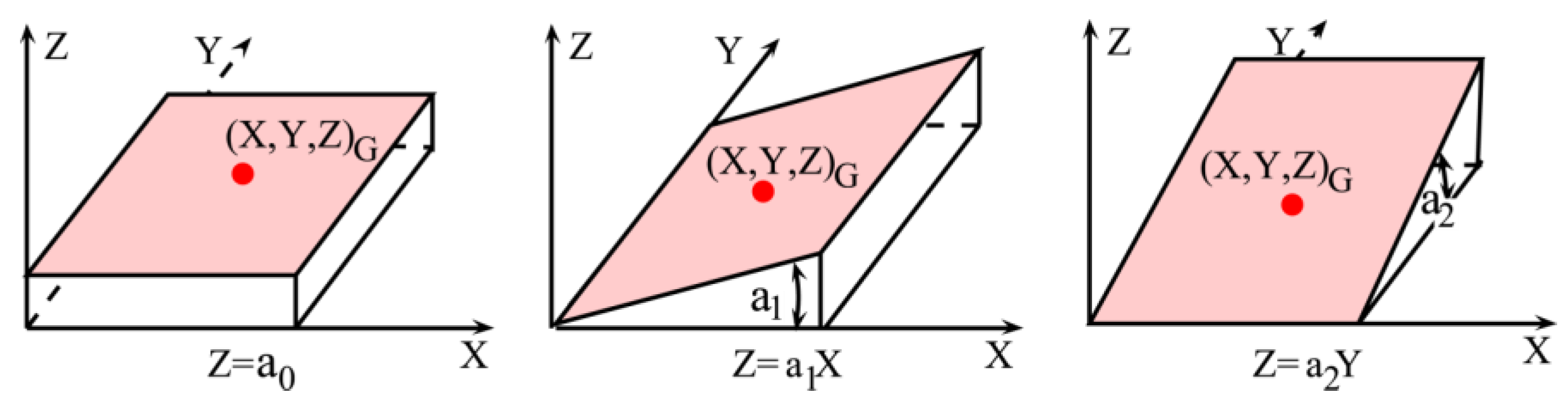
3.1. Reconstructing the Scanning Geometry

3.2. Theoretical Quality of Laser Points

3.3. Empirical Quality of Laser Points
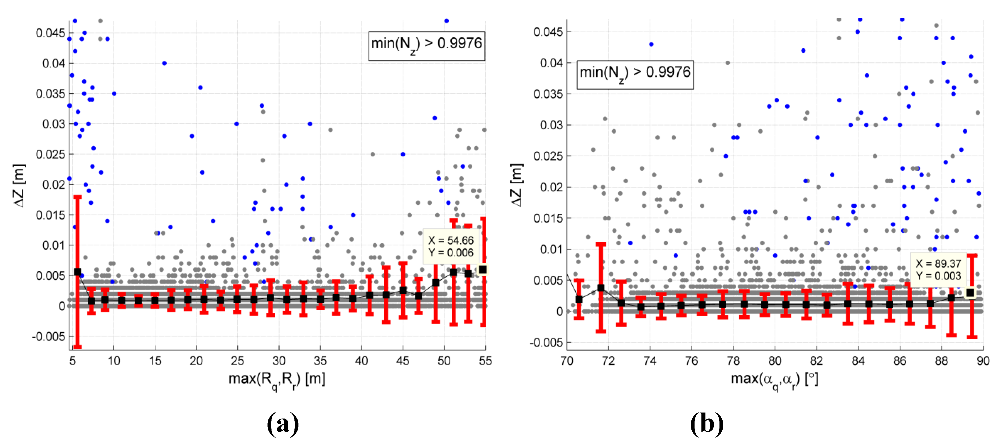
- As the footprint diameter goes to infinity when the incidence angle is 90° only laser points that have an incidence angle less than 89.9° are considered: αP < 89.9°.
- Because just the vertical component of two points is compared, points should lie on an almost horizontal plane in order to avoid the influence of surface slope on the height difference. This requirement is considered to be fulfilled if the vertical component of the unit normal vector np,z computed at each laser point, as explained in Section 3.1, is close to 1; that is: np,z ≈ 1.
- Identical points (IP) from the complete data set.
- Identical points (IP) belonging to different scanners (scanner overlap).
- Identical points (IP) belonging to overlapping drive-lines (drive-line overlap).
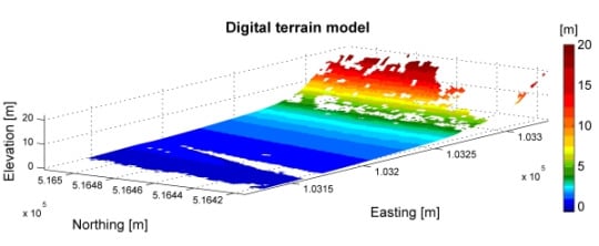
4. DTM Interpolation and Quality

5. Results and Discussion
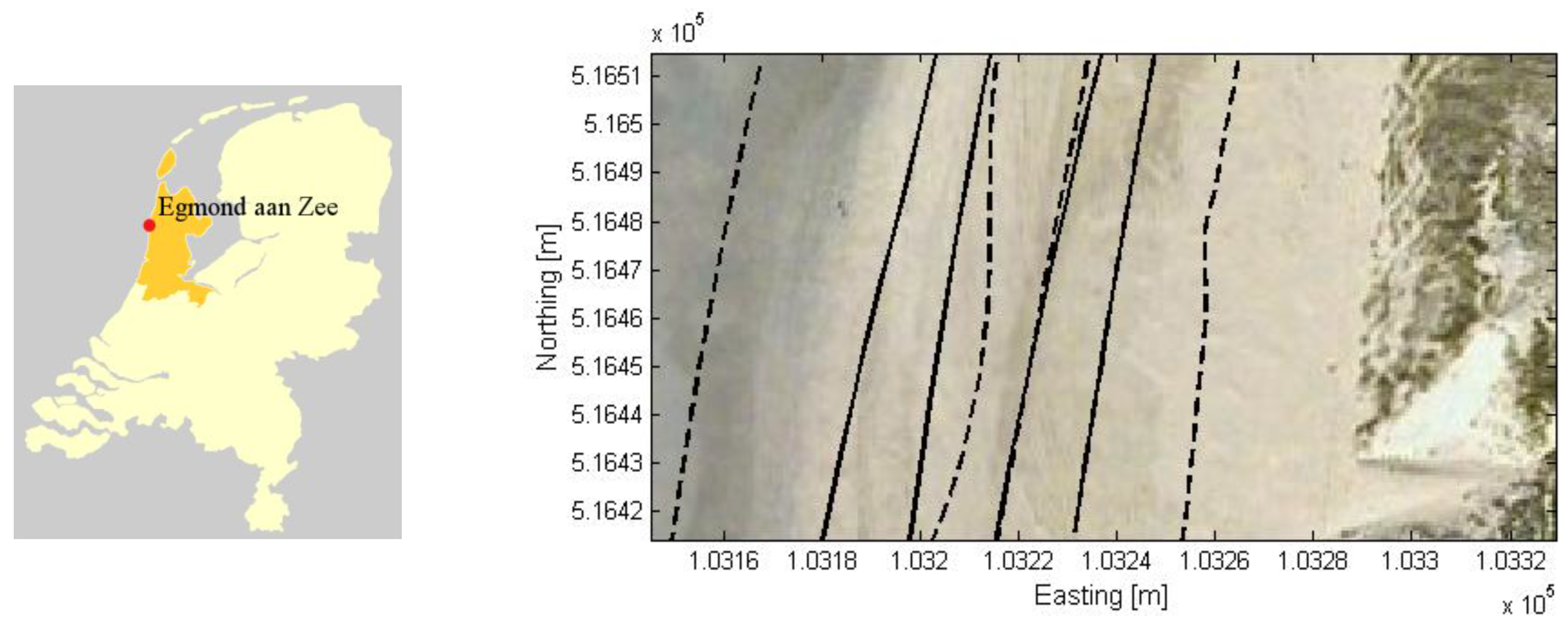
5.1. Data Description

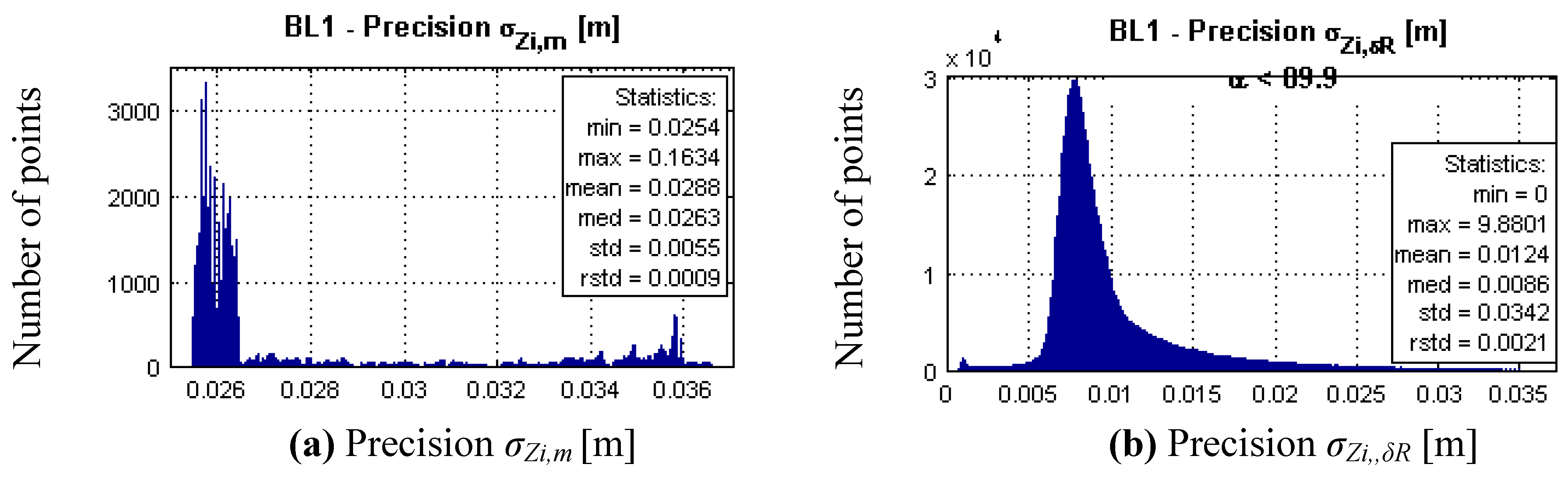
5.2. Results of Theoretical Precision

5.3. Results of Height Differences of Identical Points

| ALL | Scanner overlap | Drive-line overlap | ||
|---|---|---|---|---|
| No. of identical point pairs | 17,754 | 608 | 5,473 | |
| Height difference ΔZ [mm] | Min | −47 | −20 | −47 |
| Max | 46 | 36 | 46 | |
| Avg | 0.1 | 0.2 | 0.0 | |
| Std | 3.1 | 2.5 | 3.5 | |

5.4. Comparison of Empirical and Theoretical Height Precision
| min | max | mean | std | RMSE | ||
|---|---|---|---|---|---|---|
| Empirical | ΔZALL [m] | −0.0470 | 0.0460 | 0.0001 | 0.0031 | 0.0031 |
| Theoretical | σΔz [m] | 0.0376 | 4.8515 | 0.0573 | 0.0658 | 0.0872 |
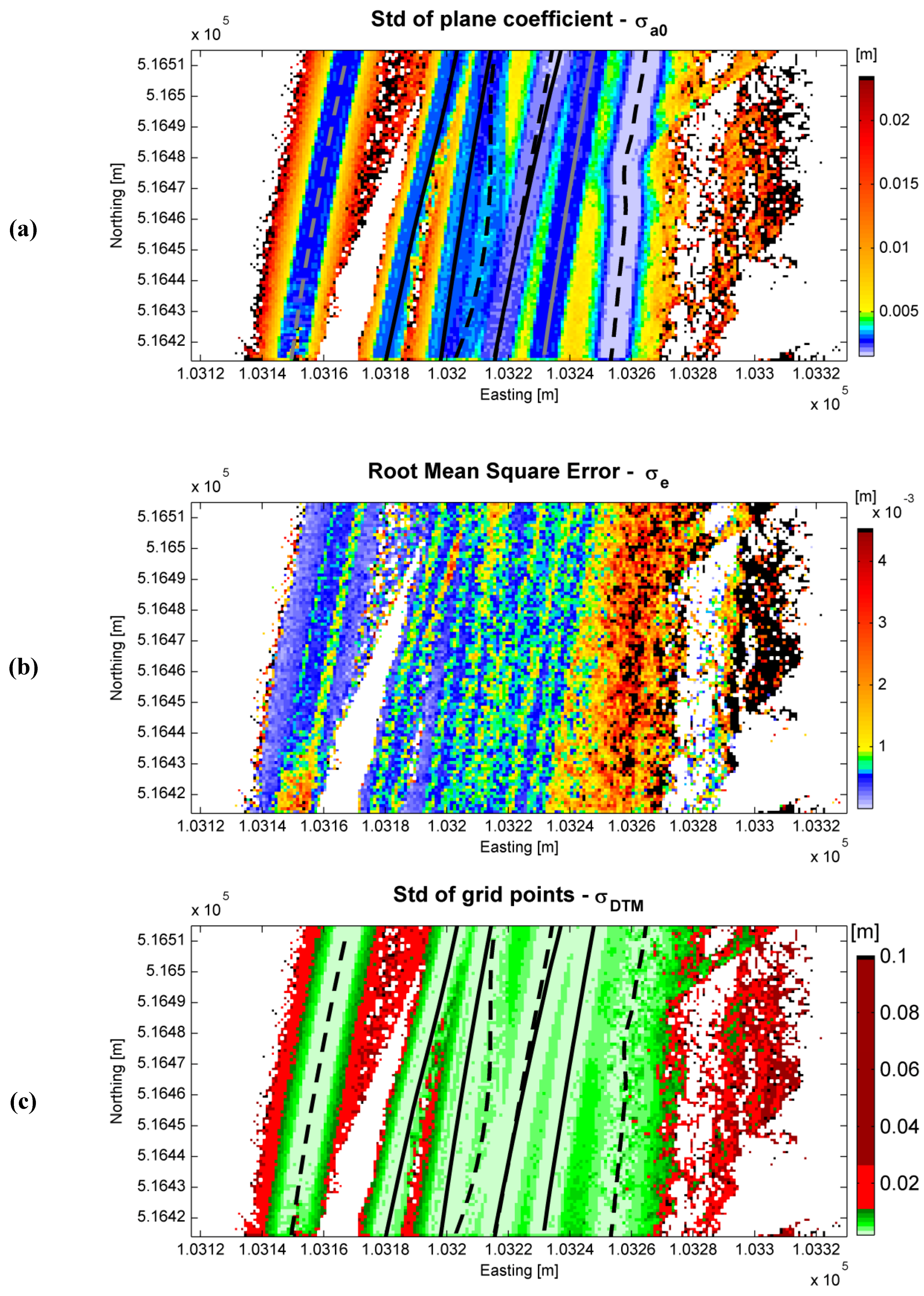
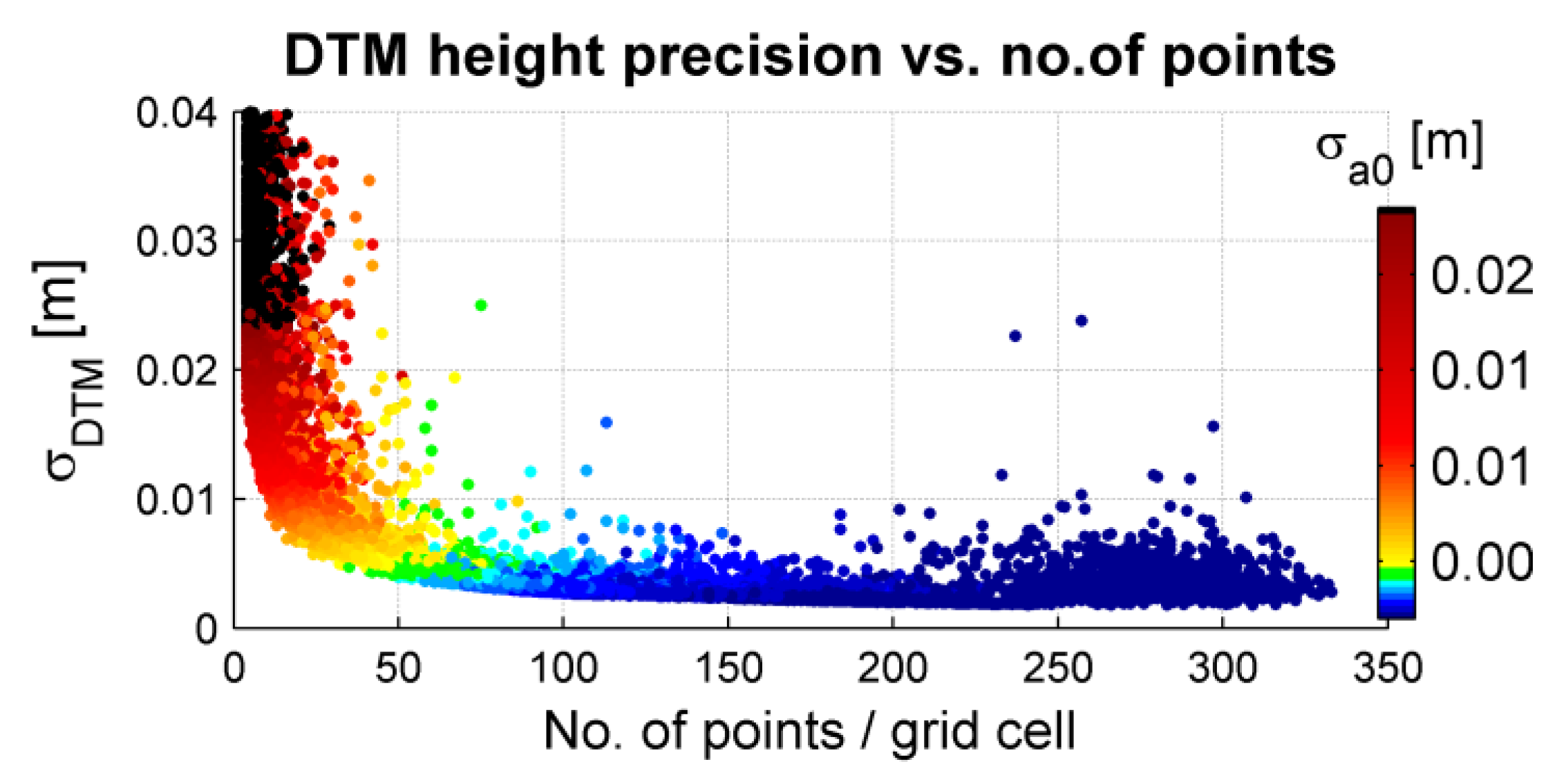
5.5. Results of DTM Interpolation and Precision Estimation
| n (FD1) | (FD2) | ZMLS | σa0 | σe | σDTM | |
|---|---|---|---|---|---|---|
| [m] | [m] | [m] | [m] | [m] | ||
| min | 4 | 0.026 | −0.19 | 0.0015 | 0.0000 | 0.0018 |
| max | 333 | 0.85 | 21.88 | 2.9 | 0.1001 | 2.9 |
| med | 69 | 0.033 | 1.25 | 0.0042 | 0.0008 | 0.0047 |
| rstd | 76 | 0.008 | 1.28 | 0.0030 | 0.0006 | 0.0030 |


6. Summary, Conclusion and Recommendations
6.1. Summary
- The LMMS measurements resulting in the measurement precision of laser points.
- The non-perpendicular scanning geometry resulting in the geometrical precision of laser points.
6.2. Conclusions
6.3. Recommendations
Acknowledgments
References and Notes
- de Ruig, J.H.M.; Hillen, R. Developments in Dutch coastline management: Conclusions from the second governmental coastal report. J. Coast. Conserv. 1997, 3, 203–210. [Google Scholar] [CrossRef]
- van Son, S.T.J.; Lindenbergh, R.C.; de Schipper, M.A.; de Vries, S.; Duijnmayer, K. Using a Personal Watercraft for monitoring Bathymetyric Changes at Storm Scale. In Proceedings of Hydro ’09, Cape Town, South Africa, 10–12 November 2009.
- Stockdon, H.F.; Doran, K.S.; Sallenger, A.H. Extraction of lidar-based Dune-Crest Elevations for use in examining vulnerability of beaches to inundation during hurricanes. J. Coast.Res. 2007, 53, 59–65. [Google Scholar] [CrossRef]
- Ellum, C.; El-Sheimy, N. Land-based mobile mapping systems. Photogramm. Eng. Remote Sensing 2002, 68, 13–17. [Google Scholar]
- Vosselman, G.; Maas, H.G. Airborne and Terrestrial Laser Scanning; Whittles Publishing: Boca Raton, FL, USA, 2010. [Google Scholar]
- Shan, J.; Toth, C.K. Topographic Laser Ranging and Scanning: Principles and Processing; Taylor & Francis Group: Boca Raton, FL, USA, 2008. [Google Scholar]
- Petrie, G. An introduction to the technology mobile mapping systems. GEOinformatics Magazine 2010, 13, 32–43. [Google Scholar]
- Barber, D.M.; Mills, J.P. Vehicle Based Waveform Laser Scanning in a Coastal Environment. In The 5th International Symposium on Mobile Mapping Technology (MMT’07), Padua, Italy, 28–31 May 2007.
- Pietro, L.S.; O’Neal, M.A.; Puleo, J.A. Developing terrestrial-lidar-based Digital Elevation Models for monitoring beach nourishment performance. J. Coast. Res. 2008, 24, 1555–1564. [Google Scholar] [CrossRef]
- Lichti, D.D.; Gordon, S.J. Error Propagation in Directly Georeferenced Terrestrial Laser Scanner Point Clouds for Cultural Heritage Recording. In FIG Working Week 2004, Athens, Greece, 23–30 May 2004.
- Habib, A.F.; Al-Durgham, M.; Kersting, A.P.; Quackenbush, P. Error Budget of Lidar Systems and Quality Control of the Derived Point Cloud. In ISPRS Congress, Beijing, China, 3–11 July 2008; Vol. 37, Part B1, pp. 203–209.
- Sande, C.v.d.; Soudarissanane, S.; Khoshelham, K. Assessment of relative accuracy of AHN-2 laser scanning data using planar features. Sensors 2010, 10, 8198–8214. [Google Scholar] [CrossRef] [PubMed]
- Kraus, K.; Karel, W.; Briese, C.; Mandlburger, G. Local accuracy measures for digital terrain models. Photogramm. Record 2006, 21, 342–354. [Google Scholar] [CrossRef]
- Giaccari, L. Fast K-Nearest Neighbors Search. 25 August 2009. Available online: http://www.advancedmcode.org/gltree.html (accessed date: 6 July 2011).
- Glennie, C.L. Rigorous 3D error analysis of kinematic scanning lidar systems. J. Appl. Geodesy 2007, 1, 147–151. [Google Scholar] [CrossRef]
- Alharthy, A.; Bethel, J.; Mikhail, E.M. Analysis and Accuracy Assessment of Airborne Laser Scanning Systems. In XXth ISPRS Congress, Istanbul, Turkey, 12–23 July 2004; pp. 144–149.
- Soudarissanane, S.; Lindenbergh, R.; Menenti, M.; Teunissen, P. Incidence Angle Influence on the Quality of Terrestrial Laser Scanning Points. In Laser Scanning ’09, Paris, France, 1–2 September 2009.
- Schaer, P.; Skaloud, J.; Landtwing, S.; Legat, K. Accuracy Estimation for Laser Point-cloud including Scanning Geometry 2007. In 5th International Symposium on Mobile Mapping Technology (MMT2007), Padua, Italy, 28–31 May 2007.
- Lichti, D.D.; Gordon, S.J.; Tipdecho, T. Error models and propagation in directly georeferenced terrestrial laser scanner networks. J. Survey. Eng. 2005, 131, 135–142. [Google Scholar] [CrossRef]
- Kremer, J.; Hunter, G. Performance of the StreetMapper Mobile LIDAR Mapping System in “Real World” Projects. In Photogrammetric Week’07; Fritsch, D., Ed.; Wichmann Verlag: Heodelberd, Germany, 2007; pp. 215–225. [Google Scholar]
- Barber, D.M.; Holland, D.; Mills, J.P. Change detection for topographic mapping using three-dimensional data structures. Int. Arch. Photogramm. Remote Sens. Spatial Inf. Sci. 2008, 37, 1177–1182. [Google Scholar]
- Lu, H. Modelling Terrain Complexity. In Advances in Digital Terrain Analysis; Lecture Notes in Geoinformation and Cartography; Zhou, Q., Lees, B., Tang, G.-a., Eds.; Springer: Berlin, Germany, 2008; pp. 159–176. [Google Scholar]
- Wackernagel, H. Multivariate Geostatistics: An Introduction with Applications, 3rd ed.; Springer: Berlin, Germany, 2003. [Google Scholar]
- Li, Z.; Zhu, Q.; Gold, C. Digital Terrain Modeling: Principles and Methodology; CRC Press: New York, NY, USA, 2005. [Google Scholar]
- Karel, W.; Kraus, K. Quality parameters of digital terrain models. In Checking and Improving of Digital Terrain Models/Reliability of Direct Georeferencing; European Spatial Data Research (EuroSDR): Utrecht, The Netherlands, 2006. [Google Scholar]
- StreetMapper. StreetMapper Mobile Mapping System. Available online: http://www.streetmapper.net (accessed on 6 July 2011).
- Geomaat. Available online: http://cms.geomaat.pageflow.nl (accessed on 6 July 2011).
- Kraus, K.; Briese, C.; Attwenger, M.; Pfeifer, N. Quality Measures for Digital Terrain Models. In XXth ISPRS Congress, Istanbul, Turkey, 12–23 July 2004.
© 2011 by the authors; licensee MDPI, Basel, Switzerland. This article is an open access article distributed under the terms and conditions of the Creative Commons Attribution license (http://creativecommons.org/licenses/by/3.0/).
Share and Cite
Bitenc, M.; Lindenbergh, R.; Khoshelham, K.; Van Waarden, A.P. Evaluation of a LIDAR Land-Based Mobile Mapping System for Monitoring Sandy Coasts. Remote Sens. 2011, 3, 1472-1491. https://doi.org/10.3390/rs3071472
Bitenc M, Lindenbergh R, Khoshelham K, Van Waarden AP. Evaluation of a LIDAR Land-Based Mobile Mapping System for Monitoring Sandy Coasts. Remote Sensing. 2011; 3(7):1472-1491. https://doi.org/10.3390/rs3071472
Chicago/Turabian StyleBitenc, Maja, Roderik Lindenbergh, Kourosh Khoshelham, and A. Pieter Van Waarden. 2011. "Evaluation of a LIDAR Land-Based Mobile Mapping System for Monitoring Sandy Coasts" Remote Sensing 3, no. 7: 1472-1491. https://doi.org/10.3390/rs3071472