1. Introduction
Detection and tracking of dynamic objects has become an important field for the correct development of many multidisciplinary applications, such as traffic supervision [
1], autonomous robot navigation [
2,
3], and surveillance of large facilities [
4]. This article is primarily focused on detection of moving objects from aerial vehicles for surveillance, although other potential applications could also benefit from the results.
The background to dynamic image analysis from moving vehicles can be divided into four main topics [
5]: background subtraction methods, sparse features tracking methods, background modeling techniques and robot motion models.
Background subtraction methods, mostly used with stationary cameras, separate foreground moving objects from the background [
6,
7]. Other approaches use stereo disparity background models [
8] for people tracking. Kalafatic
et al. [
9] propose a real-time system to detect and track quasi-rigid moving objects for pharmaceutical purposes that is based on computing sparse optical flow along contours. Zhang
et al. [
10] use polar-log images to enhance the performance of optical flow estimation methods. In this latter case, the optical flow is only computed along the edge of the moving features. Since these two methods use static cameras, the moving contours are easily determined since the static pixels do not change their position in the image.
These techniques are not sufficient when the camera is attached to a moving robot. Under these recording conditions, adaptive background models [
11] have been used because they can incorporate changes in the images produced by illumination variations in outdoor scenes or background changes due to small camera motions. However, these methods are not robust when the scene changes rapidly, and then they usually fail. To improve the detection process under such conditions, the camera motion model can be constrained. Thus, Franke
et al. [
12] developed an obstacle detection method for urban traffic situations by assuming forward camera motion, while dealing with rotation by means of rotation motion templates. Other methods include multiple degrees of freedom for egomotion calculation, although in this case most of the research is focused on cameras that are mounted on ground vehicles, and so there are some constraints on their movement [
13]. Improved sensors, such as LIDARS, have also been used to detect and track dynamic objects [
14].
Techniques for tracking point features have been used in ground-level moving platforms, using both monocular [
15] and stereo [
16] approaches to determine the movement of the robot and to construct maps of the terrain [
17]. Jia
et al. [
18] proposed an extended Kalman filter algorithm to estimate the state of a target. Optical flow vectors, color features and stereo pair disparities were used as visual features. Each of these approaches for ground moving vehicles impose a different set of constrains for the determination of the optical flow. For aerial vehicles quite different approaches are required because of their additional freedom of movement. Some of the most common methods are described below.
As shown by Miller
et al. [
19], one possible approach is to use background subtraction methods with a combination of intensity threshold (for IR imagery), motion compensation and pattern classification. Chung
et al. [
20] applied accumulative frame differencing to detect the pixels with motion and combined these pixels with homogeneous regions in the frame obtained by image segmentation. Other methods use optical flow as the main analysis technique. For example, Samija
et al. [
21] used a segmentation of the optical flow in an omnidirectional camera. In this case the movement of the camera was known and the vectors of the optical flow were mapped on a sphere. Using optical flow methods, Suganuma
et al. [
22] presented a stereo system to obtain occupancy grids and to determine direction and speed of dynamic objects for safe driving environments.
Herein, we have developed a new method that combines egomotion determination based on static point features with optical flow comparison to determine pixels that belong to dynamic objects. Chung
et al. [
20] proposed a frame differencing procedure that would not work in our case due to the high frequency vibrations in the movement of currently available commercial UAVs. Meanwhile, our method only tracks single static features to determine the movement of the camera. Like Sugamanuma
et al. [
22] we use optical flows techniques, but instead of a stereo vision system, we only need a single camera to obtain a list of all possible dynamic objects in the environment. Samija
et al. [
21] also employed a single camera, but the movement of the camera was known prior to the optical flow calculation. In our case the camera motion estimation is obtained without any further sensor. Another advantage of our method is that, due to its mathematical simplicity, it can be executed in real-time on the onboard UAV computer.
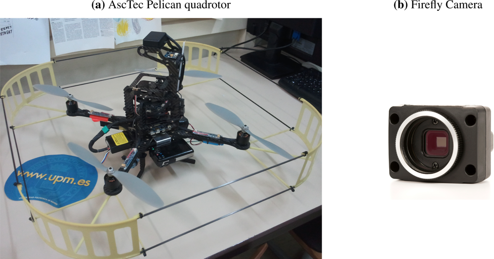
The paper is organized as follows. Section 2 presents a general overview of the algorithm and briefly discusses each part, as well as the interconnections between them. In Section 3 we describe the new methods proposed to calculate the optical flows, together with the heuristic rules defined to compare two optical flows. Section 4 discusses the object definition procedure and the filtering and matching techniques used to track the real dynamic objects. In the results Section 5 we present the hardware setup used to test these algorithms and the results obtained. These tests have been carried out with a commercial quadrotor taking videos of a landscape field. Finally, Section 6 highlights conclusions, advantages, as well as the shortcomings of the procedure. We also point out the different fields of application where this technology might be applied. Future works aiming to add some additional functionality to the algorithm are also mentioned.
2. Methodology Overview
The main problem to solve when trying to detect moving objects from a flying UAV is to separate the changes in the image caused by the movement of the vehicle from those caused by dynamic objects. Although this problem is not limited to aerial vehicles, it represents an additional difficulty with UAVs since they have more degrees of freedom. In this case the input data adopts the form of a continuous flow of images produced by a single grayscale camera. From these images we have to obtain the position and velocity of the dynamic objects in the scene.
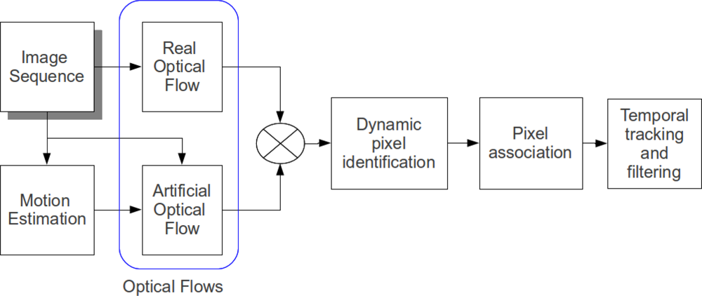
The main part of the new proposed methodology consists of comparing an artificial optical flow based on the movement of the camera with the real optical flow, and tracking the discrepancies. The complete architecture of the system can be appreciated in
Figure 1. The core of this algorithm is the calculation of an artificial optical flow and its comparison with the real optical flow (highlighted in
Figure 1). We have developed this method because it permits analysis of the whole image using a very small set of pixels in the actual process of comparison. The extrapolation of the information obtained using this set is enough for detecting and tracking moving objects in the whole image.
In addition to the overall scheme, the method contains the following elements intended to carry out different functions:
Image Sequence: In general, our method should work with any type of image sequence, provided that the resolution is adequate. Both triple and mono-color channel images can be handled.
Motion Estimation: A method to obtain the estimated movement of the camera is crucial for the performance of the algorithm. Klein
et al. [
23] have developed a method of estimating camera pose in an unknown scene with a single handheld camera for small augmented reality (AR) workspaces using a Parallel Tracking and Mapping (PTAM) algorithm. It consists of two parallel threads for tracking and mapping a previously unknown scene. This method has been modified here to adapt it to our working conditions. For these purposes, the most important thread is the tracking one, which provides an estimation of the camera position in the map that is being dynamically generated and updated by the second thread. The map consists of 3D point features that are tracked through time in previously observed video frames. This way of collecting data permits the use of batch optimization techniques that are rather uncommon in real-time systems because they are computationally expensive. This system is designed to produce detailed maps with thousands of features in small restricted areas such as an office. It also enables tracking the features at the frame rate with great accuracy and robustness. Further details of this method can be found in this previous work [
23].
Optical flows: For the image sequence, both a real and an artificial optical flow are obtained. This implies a careful selection of the pixels which are later on used to calculate the optical flows. This selection process is carried out by using procedures adapted from a tree based 9 point FAST feature detection process described by Rosten
et al. in [
24]. Generally, the initially selected group of features is too large to be used in real-time, so that a reduced set of these features must be chosen. To accomplish this reduction, a non-maximal suppression of the FAST features is carried out. The choice of using two optical flows is motivated by the need to enhance the differences produced by dynamic objects. As described in Section 3, the real optical flow is calculated by using the iterative Lucas–Kanade method with pyramids [
25], while the artificial optical flow is calculated by means of a homography.
Identification of dynamic pixels: This part of the work incorporates a new approach for identifying moving objects from a moving camera. The identification of the pixels that might belong to a dynamic object moving in the image is obtained by comparing the real and the artificial optical flows. Discrepancies between the two optical flows are then calculated using a two stage filter. Since an optical flow is a vector field, the first computational step consists of analyzing the direction of the flows in each pixel. Great variations in their direction (more than 20°) indicate a discrepancy and then the pixel is flagged as dynamic. The second step analyzes the magnitude of the vector looking for differences greater than a predefined threshold (in our case more than 30%). These pixels are also flagged as dynamic.
Pixel association: The comparison of the flows yields a subset of vectors of the real optical flow that might belong to dynamic objects. These elements may come from both actual dynamic objects and also from spurious events, or may just be caused by errors from the optical flow calculation process. Possible sources of errors are, for example, patterned textures, homogeneous surfaces, etc. To discard these erroneous pixels and associate the others into dynamic objects, different filtering techniques are used. To minimize the processed information, the groups of vectors are represented by a rectangular area, which is described by a center coordinate and two dimensions. A list of the potential dynamic objects representations is generated and stored for further filtering and temporal tracking.
Filtering and temporal tracking of dynamic objects: The process described above relies on the comparison of two subsequent images of the selected sequence. To efficiently track dynamic objects and discard any possible misidentification, temporal constraints must be incorporated into the algorithm.
In the following sections we will develop in more detail the basic principles of this new approach. The first step in this process is to show how the optical flows are calculated and which heuristic rules have been defined to compare them.
3. Motion through Optical Flow Difference
In this section we describe the process of identifying the pixels that might belong to a dynamic object. This is done by calculating and comparing the real optical flow and an artificially calculated one. This part is the core of the algorithm and is based on a new concept which, to our knowledge, has not been previously used in the literature [
6,
7,
13,
20,
21]. Thus, contrary to the method in [
6] and [
7], our method uses a free moving camera instead of a stationary one. In [
13] moving cameras were mounted on terrestrial vehicles but their movements were constrained and therefore the experimental conditions are not applicable to UAV. Our method, intended to be used with images taken from an UAV, has to work when there are no movement constraints and with real-time analysis. Due to the complexity of the recording conditions, the use of optical flow techniques provides a means to analyze the whole set of video images by focusing the calculations on a small number of selected pixels.
The PTAM algorithm is running onboard at a maximum frequency of 10 Hz [
26]. Since the input image sequence is streaming at 30 Hz, this means that the motion estimator is working with a third of the available images. Even that number of image frames is excessive for our purposes. To tackle with this problem, we adapt the working frequency of our algorithm to the movement of the UAV. When the UAV is moving very fast we work at the highest available frequency (10 Hz), but if the movement is slow we wait for the UAV to move a certain distance to permit changes in the image. We define a minimum working frequency of 5 Hz for the case that the UAV is staying over the same place (hovering).
We describe below the calculation process of the two optical flows and the rules imposed for their straightforward comparison.
3.1. Real Optical Flow
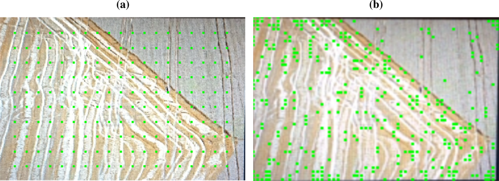
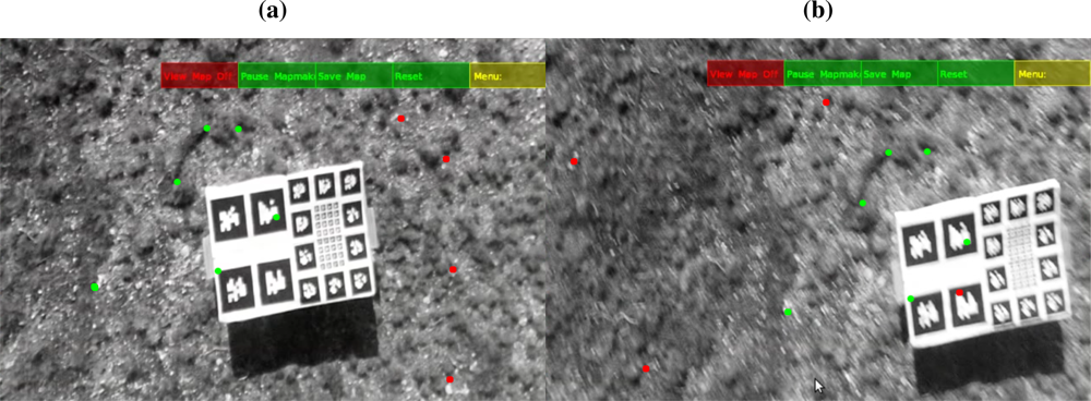
To obtain the real optical flow, the first step is to select the group of features that should be tracked in two subsequent frames. We have used two different approaches to determine the feature set. They have been applied to the same frame with the results shown in
Figure 2 taken as an example. As shown in
Figure 2(a) the first approach relies on the classical method of selecting pixels by defining a regular grid in the image. These pixels are selected merely based on their position, without any consideration to their contrast or surrounding pixels. The main problem by this approach is that pixels with bad tracking features (e.g., pixels from a homogeneous patterned area, a smooth surface with little or no contrast,
etc.) have the same probability to be selected as good features (e.g., pixels from rough surfaces, natural landscapes with vegetation,
etc.). Although this method may present some restrictions when applied in complex real situations, we have included it here because we obtained good results in simple cases.
As shown in
Figure 2(b), the second approach consists of applying the 9 point FAST feature detection developed by Rosten
et al. in [
24]. This algorithm looks for small points of interest with variations in two dimensions. Such points often arise as the result of geometric discontinuities, such as the corners of real world objects, although they can also arise from small patches of texture. This second procedure also presents some limitations, particularly when used with images of different areas, some with highly heterogeneous textures and others with little contrast and very homogeneous. In this case, the homogeneous area would be neglected and only pixels of the highly featured areas would be selected. Nevertheless, for the purposes of the present work, this method is quite appropriate because of the particular characteristics of the examined terrain consisting of fields and vegetated areas lacking large homogeneous zones. Under these conditions the pixels with the best tracking features would be more evenly distributed through the whole image. Although a feature tracking process is carried out by the PTAM algorithm, we must note that the features tracked by this algorithm are static. Since we want to detect dynamic objects, a new group of features needs to be selected for each image. Alternative feature selection techniques, such as SIFT (
Scale-Invariant Feature Transform) [
27], SURF (
Speeded Up Robust Features) [
28] or KLT (
Kanade–Lucas–Tomasi) [
29] could have been used. A comparative study of these methods has been recently performed by Bonin
et al. [
30], and although they conclude that for their application the most efficient method was KLT, we found that FAST feature selection best suits our purposes. This is likely because FAST feature selection is more suitable for high frame rate video streams and rapid motions, as noted by those authors.
Once the selection of the pixels has been completed, the optical flow is calculated by applying the iterative Lucas–Kanade method with pyramids [
25].
3.2. Artificial Optical Flow
From the pixel set selected to obtain the real optical flow, an artificial flow represents the position of all these pixels projected mathematically in the next frame by considering the movement of the camera between the two images. This movement is represented by a rotation and a translation (R, T) obtained by the PTAM algorithm. Using an artificial flow we get information about the change in the position of these pixels resulting exclusively from the movement of the camera, thus neglecting any possible dynamic objects in the image.
Typically, the homography matrix
H is calculated by using a variation of the RANSAC algorithm [
31,
32], which iterates the calculation with a selection of pixels trying to maximize the number of inliers. For our application we prefer to obtain the matrix
H directly from the motion estimation because it avoids such an iterative process, which does not seem necessary as our method appears to cope effectively with outliers.
To obtain the artificial optical flow based on the camera motion we have used a conventional homography projection [
33]. A typical homography projects the position of a given point in a plane from one camera coordinate frame into that of another camera. In our case, some particular assumptions have been made to simplify and speed up the projection process. The most important one assumes that the ground is not significantly inclined, so that the average slope can be considered close to zero. Small relief changes, in the order of 40–50 cm, do not affect the algorithm ability to detect dynamic objects, as long as the long distance average slope is close to zero.
Mathematically we deal with the homography in the following way. For two subsequent frames identified as
k and
k + 1, the projection of a point
pi with coordinates in the first frame [
xk, yk] can be calculated as shown in
Equation (1). In this equation
Rk,k+1 and
tk,k+1 correspond to the rotation and translation between the camera coordinate frames
k and
k + 1;
nT is the vector perpendicular to the ground plane; and
d̄ is the mean distance from the camera position to the ground plane. An important assumption for this calculation is that the altitude of the camera does not vary much between frame
k and
k + 1 (note that the elapsed time between frames is at most 1/5 s).
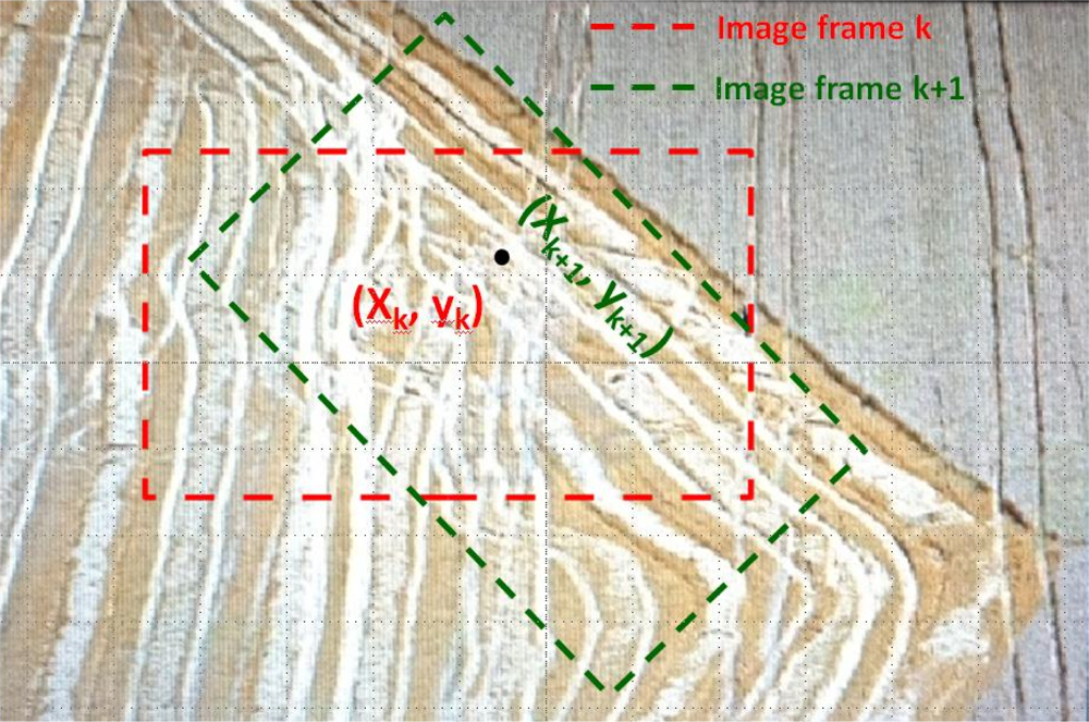
An example of the artificial flow calculation is depicted in
Figure 3. In this figure it is shown how the position (
xk,
yk) of a given pixel in an image is projected by using
Equation (1) into a new coordinate frame defined by the new position of the camera. For this example we have assumed that the camera has rotated a certain angle and translated parallel to the ground. In the global coordinate frame the point has not changed its position, but in the images’ coordinate frames the position of the point has changed from (
xk,
yk) to (
xk+1,
yk+1).
3.3. Identification of Dynamic Pixels
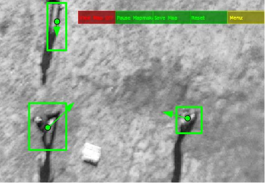
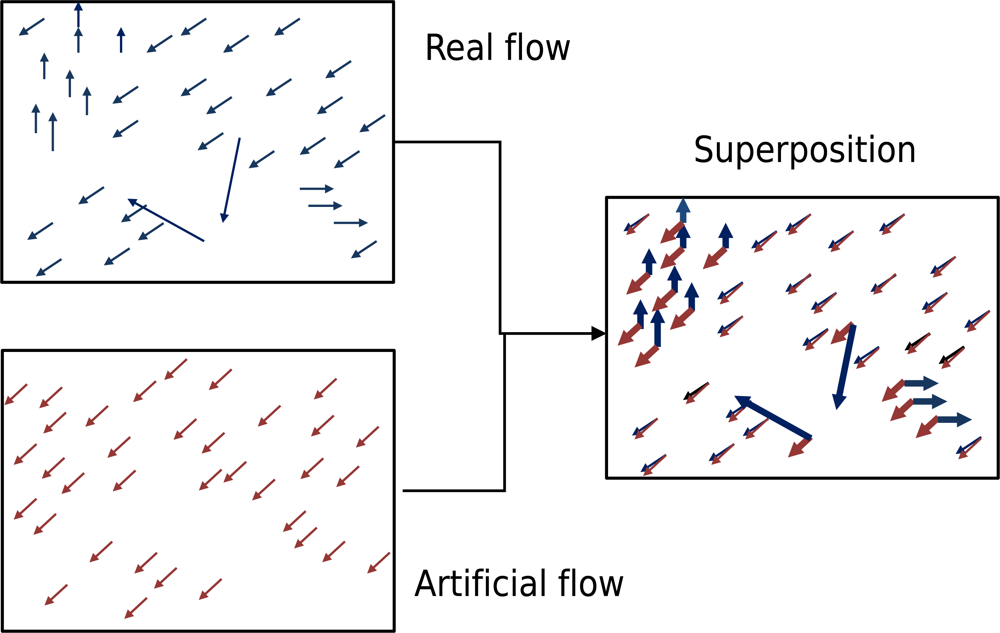
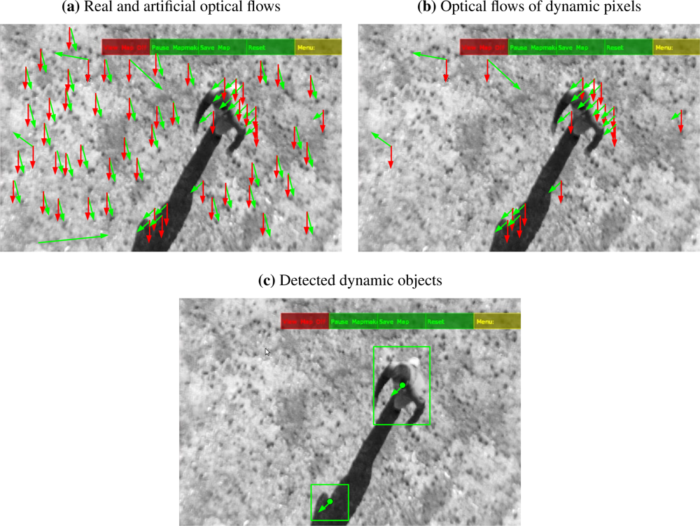
The dynamic character of a pixel is deduced by the comparison of the two previously calculated optical flows.
Figure 4 shows a series of illustrations corresponding to, respectively, a real optical flow, an artificial optical flow and their superposition into the same image. For this comparison we assume that moving objects were present in the scene. The real optical flow shows some vectors that point clearly in a different direction than the rest.
In general, there is always an offset between the real and the artificial flows. This is caused by the intrinsic error in the estimation of the position of the camera. However, there are points where that difference is clearly higher than the average. These pixels are highlighted in the superposition image of the flows. In principle, these points could be associated with a moving object. In the following sections we will see that not all of these points correspond to actual dynamic objects and that a suitable discrimination procedure has to be set up.
In general, to classify the pixels in the optical flows as moving or static, a specific procedure taking into account both their angles and modules is applied to each pair of vectors.
Calculation of the angle α formed by each vector with the camera coordinate frame. This yields the vector angles of both the real optical flow αr and the artificial one αa.
Comparison of the angle difference Δα = |αr − αa| with a predefined critical threshold αt (we use 20° for this threshold, although this parameter should be adjusted depending on the expected average altitude of the UAV). A possible way of dynamically calculating this threshold is to obtain the statistical mode from all angle differences. If Δα > αt the pixel is flagged as dynamic.
If Δα < αt the vectors modules are then compared. Although complicated statistical methods can be implemented to obtain a module difference threshold, for simplicity and to speed up the calculations, we have assumed a fixed threshold value of ± 30% with respect to the artificial optical flow.
As a result of this filtering process a group of vectors of the real optical flow is flagged as dynamic. To proceed with the calculations it is still necessary to group them spatially in the image. It may happen that some of the vectors appear isolated in the image. Commonly they are outliers due to uncontrolled fluctuations or other errors and are discarded.
4. Object Definition, Filtering and Tracking
In this section we describe the procedure developed to convert a list of pixels marked as dynamic into a list of moving objects currently present in the image. Additionally this part of the algorithm aims at filtering those objects and tracking them through time.
4.1. Object Definition through Pixel Association
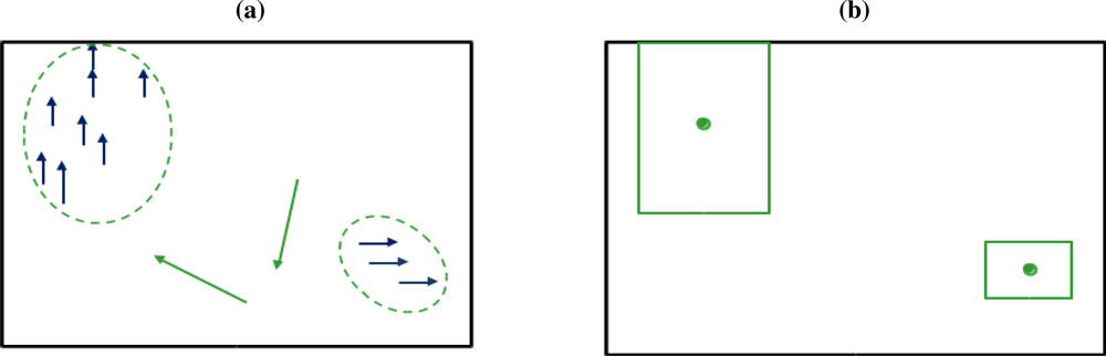
In general, dynamic objects include a considerable number of pixels. This number depends on the size of the object and the altitude of the UAV for each frame. To handle such variety of possibilities, in this part of the algorithm different criteria are defined to associate the pixels flagged as dynamic into possible moving objects and to discard those caused by errors and outliers. Typically these errors and outliers are caused by pairing failures during the application of the Lucas–Kanade method to calculate the optical flow. An example is schematically shown in
Figure 5. The associated vectors are grouped into two different elements and reduced to a rectangle as schematically represented in
Figure 5(b). There are also some isolated vectors that, although initially identified as dynamic pixels, are discarded because they do not form a group with the critical size required to be classified as part of a moving object. Another criterion to remove these vectors is that they point in quite different directions.
Mathematically the association process is carried out by performing the following operations:
Discard large module vectors (i.e., |v| > 0.3 * ImageWidth).
Remove single isolated dynamic pixels.
Group vectors with similar angles and magnitudes positioned in a nearby area into a single moving object. This grouping process is carried out as follows:
Discard groups with fewer vectors than a minimum threshold (i.e., we discard groups with fewer than 5 points).
Once a set of dynamic pixels has been grouped into a moving object, its basic characteristics must be deduced. Namely, we extract information about the size (length and width) and the position of the center. At this stage, using sensor fusion techniques, color and temperature could be also added to the algorithm and treated in a similar fashion. For further computation the center and size of the object are used to create a virtual rectangle in the position of the object as represented in
Figure 5(b). This reduction of information enables the fast real-time processing which is necessary for onboard computation.
At the end of this step there is a list of actual possible moving objects La. This list is checked by the algorithm to match the objects it contains with the global dynamic object list Lg. To initialize Lg, the first La, determined by comparing the two first video frames, is taken as the initial list.
4.2. Object Temporal Tracking and Spatial Filtering
First, the algorithm implements a matching method to pair the objects in
La with those in
Lg. This method is based on an Extended Kalman Filter (EKF). We define the state of the system as all the states of each object
xi = [
x,
y,
size,
R,
G,
B,
T] in
Lg; where (
x,
y) are the coordinates of the position of the center of the object;
size is the maximum value between the length and the width obtained by the algorithm;
R,
G,
B are the color of the object obtained by sensor fusion techniques; and
T is the mean temperature of the object (supposing we had this information). We use the Extended Kalman filter to predict the next state of the system. This calculation assumes a constant velocity movement model to determine the position and assumes a constant behavior for the other variables. To pair the objects from
Lg with those in
La we use the Mahalanobis distance, as shown in
Equation (2). This procedure allows us to determine the similarities between two multidimensional variables, in this case the predicted state for object i (
) and the measurements obtained for object j (
), using the variance (
) for each variable (
v) obtained during the EKF process.
The pairs with the smallest distances are then selected according to the pairing
Algorithm 1.
Up to now the algorithm has been dealing with pairs of consecutive image frames. For the following steps a longer time scale must be considered. The previous analysis has introduced new information for the objects in Lg and even new objects might have been added to this list. Therefore, as the recording time elapses, new information must be filtered. In the global list there are two types of object. The first set includes objects that have been tracked over long periods of time or distances. This object information is being transmitted to the central base of operations or to other robots in the network. The objects in the second set have been detected only recently and therefore have been present in the list for a short period of time. Only when they have been tracked for a predefined period of time or distance (2 s or 2 m), it is concluded that they are real moving objects in the scene. They are then qualified for the first set of objects in the global list and are also transmitted to the other components of the system (the central base or the other robots, depending on the case). This process is required to avoid an unnecessary growth in the dimension of the list being transmitted due to including objects that might be produced from short time misdetections.
Algorithm 1.
Pairing of objects lists
Algorithm 1.
Pairing of objects lists
| Require: Actual Object List (La) with na objects |
| Require: Global Object List (Lg) with ng objects |
| Ensure: na > 0 ∨ ng > 0 |
| Prepare na × ng pairs: PossiblePairs |
| Calculate distance between objects in each pair according to Equation (2) |
| SelectedPairs: Selected Pairs List |
| while Size(SelectedPairs) < min(na, ng) do |
| Select pair with minimum distance |
| if Any of the objects is already in SelectedPairs then |
| Eliminate pair from PossiblePairs |
| else |
| Include pair in SelectedPairs |
| end if |
| end while |
During a real recording process, there might be several situations which lead to identifying unreal moving objects. A typical example might occur when on a terrain there are elements with a high aspect ratio (e.g., trees, high fences,
etc). To remove these faulty objects from the list of real moving objects, we implement in the algorithm basic tracking criteria that compare the position of the objects through time and eliminate those which are, in fact, static. For objects of this second category to become part of the first category, they must comply, at least, with the two next rules:
The first rule eliminates unlikely but possible groups of vectors in the same area due to patterned surfaces. The second rule applies to objects oscillating around a center without displacing a long distance. A clear example of this situation would be a bush under the action of the wind. If a certain moving object does not meet these two criteria it is eliminated from Lg.
Additionally, for a UAV taking images for a long time, Lg might become too large to be reasonably handled. This means that we need to implement a procedure to reduce the size of the list by eliminating objects that have not been detected for a very long time. To remove an object from the list we select a maximum time. This time can be adjusted for each application as a function of computation capabilities that, acting as a bottleneck, restrict the size of the list. However, we must consider that the time period must be compatible with frequent circumstances in the detection of moving objects such as occlusions and/or crossings.
Another possibility for tracking the objects could be to define a region of interest (ROI) in the image and track the keypoint features in the ROIs with local descriptors combined with robust motion estimation as proposed by Garcia
et al. [
35]. We have chosen our method firstly because it does not rely on feature tracking to follow the objects trajectories and secondly because the information produced by our method can be easily shared with other robots, which will be necessary in a security and surveillance system.
6. Conclusions and Remarks
In this work we present a new approach to detect and track moving objects from a UAV. For this purpose we have developed a new optical flow technique that has proven effective to identify real moving objects moving on a real landscape.
Image sequences taken from aerial vehicles have no static elements due to the intrinsic movements and vibrations of the UAV. Through this new method we have been able to differentiate between the changes in the images due to the movements of the UAV and the changes actually produced by the dynamic objects moving in the scene.
The techniques and algorithms presented in this paper incorporate an innovative approach. Estimated camera motion is used to calculate an artificial optical flow, which is compared to the real optical flow. Although mathematically simple, this method has proven successful in determining divergences in the real optical flow, leading to what we later on identify as dynamic objects. An additional advantage of our method is the use of a single camera, without the need of other sensors, to track static features in the ground and to estimate the camera motion. Since any moving object will have a different optical flow behavior than the optical flow based on the camera motion, this algorithm allows us to detect any moving object in the camera stream regardless of its direction of movement.
The developed technique is expected to be useful for surveillance applications in external critical facilities (e.g., nuclear plants, industrial storage facilities, solar energy plants, etc.). However, the algorithms could also be used for cattle tracking in agroindustrial environments or wild animal surveillance for ecological control activities. Another large field of applications relates to the defense industry, for example to track potential threats to critical facilities and infrastructures of national interest.
However, under certain circumstances, the procedure might have some shortcomings. Although these limitations do not hamper the practical use of our method, it is worthy to mention them to be aware of the range of applications and the possible solutions. Some limitations relate to the minimum velocity and size of the objects to be detected and with the maximum flight altitude of the UAV. Of course these three parameters are intimately linked. To minimize these restrictions, the algorithm parameters must be defined specifically for each practical case after a careful assessment of the real scenario where our technology is to be applied. Another type of shortcoming that could be devised for this type of technology is inherent to the use of a light UAV. These vehicles can be easily displaced by large unexpected wind blasts. If such a situation occurs, the UAV will be displaced suddenly by a great distance and might lose its tracking of static references on the ground. To return to a normal work cycle the UAV should be manually directed to a previously known area.
A possible and feasible solution for these problems is to integrate the position estimate given by the PTAM algorithm provided by Klein
et al. [
23] with the position measurements obtained from other sensors, such as IMU or GPS. Work is being carried out at present in our group along this line. Further improvements on which we are also working consist of applying artificial vision techniques such as contour definitions and pattern recognition.

 ,
, 


