A Novel Methodology to Estimate Single-Tree Biophysical Parameters from 3D Digital Imagery Compared to Aerial Laser Scanner Data


Abstract
:
1. Introduction
2. Materials and Methods
2.1. Study Site Field Data Measurements

| Forest variable | Average | Max. | Min. | SD |
|---|---|---|---|---|
| Trunk diameter (cm) | 39.01 | 79.7 | 11.00 | 12.19 |
| Trunk height (m) | 1.78 | 3.50 | 0.00 | 0.49 |
| Tree height (m) | 6.61 | 10.50 | 2.00 | 1.36 |
| Crown diameter (m) | 9.10 | 16.00 | 4.05 | 2.57 |
| LAI | 1.00 | 1.69 | 0.49 | 0.34 |
| Density (trees/ha) | 47.74 |
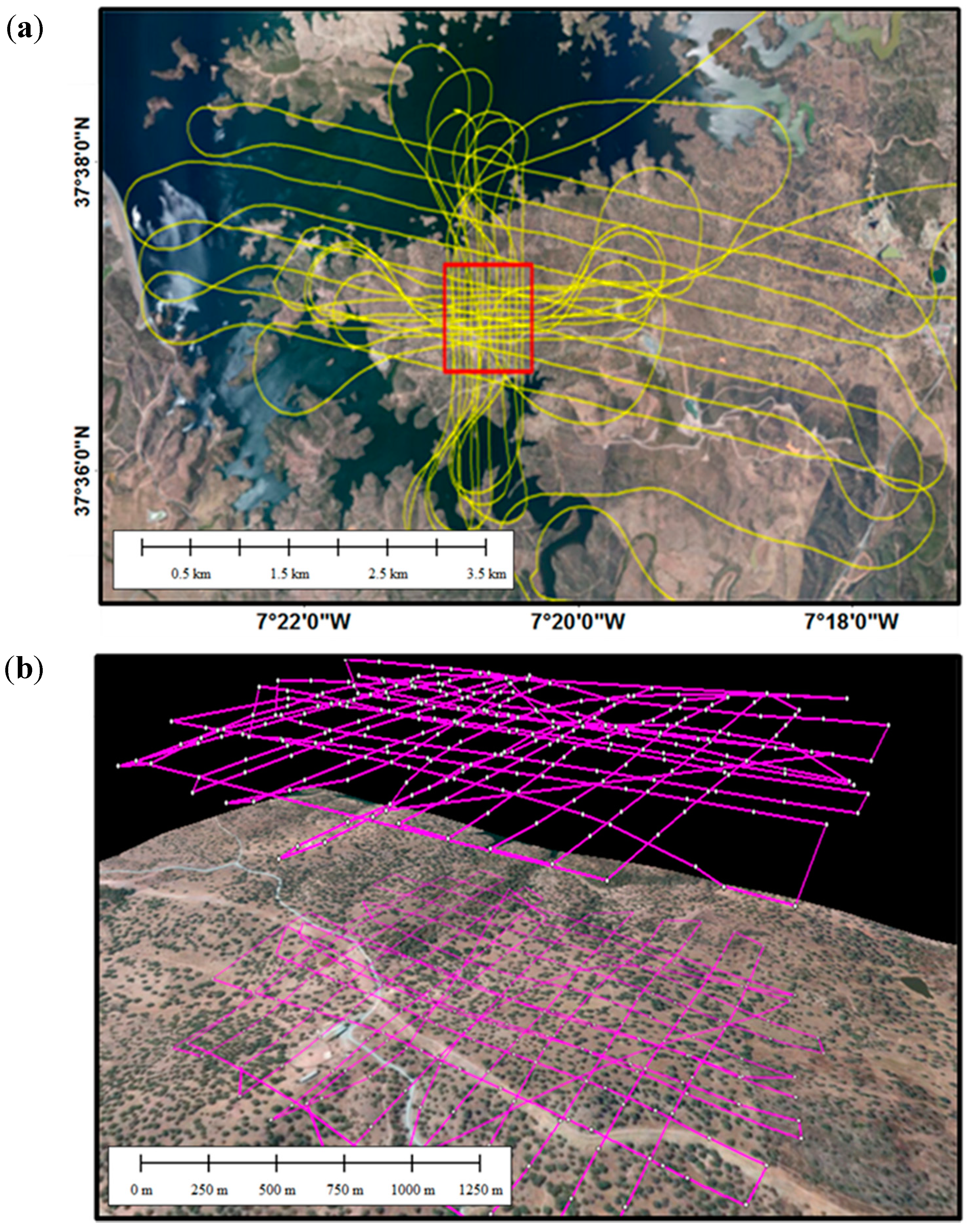
2.2. DAI and ALS Data Acquisition

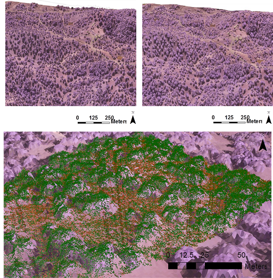
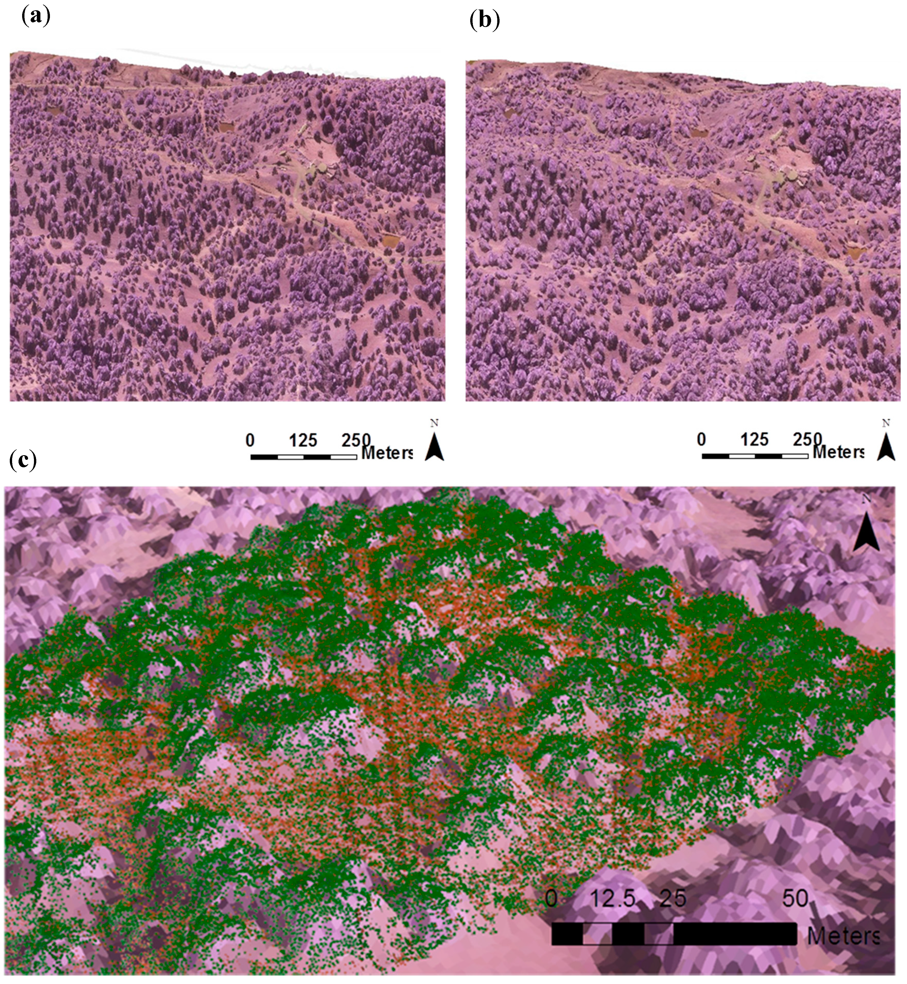
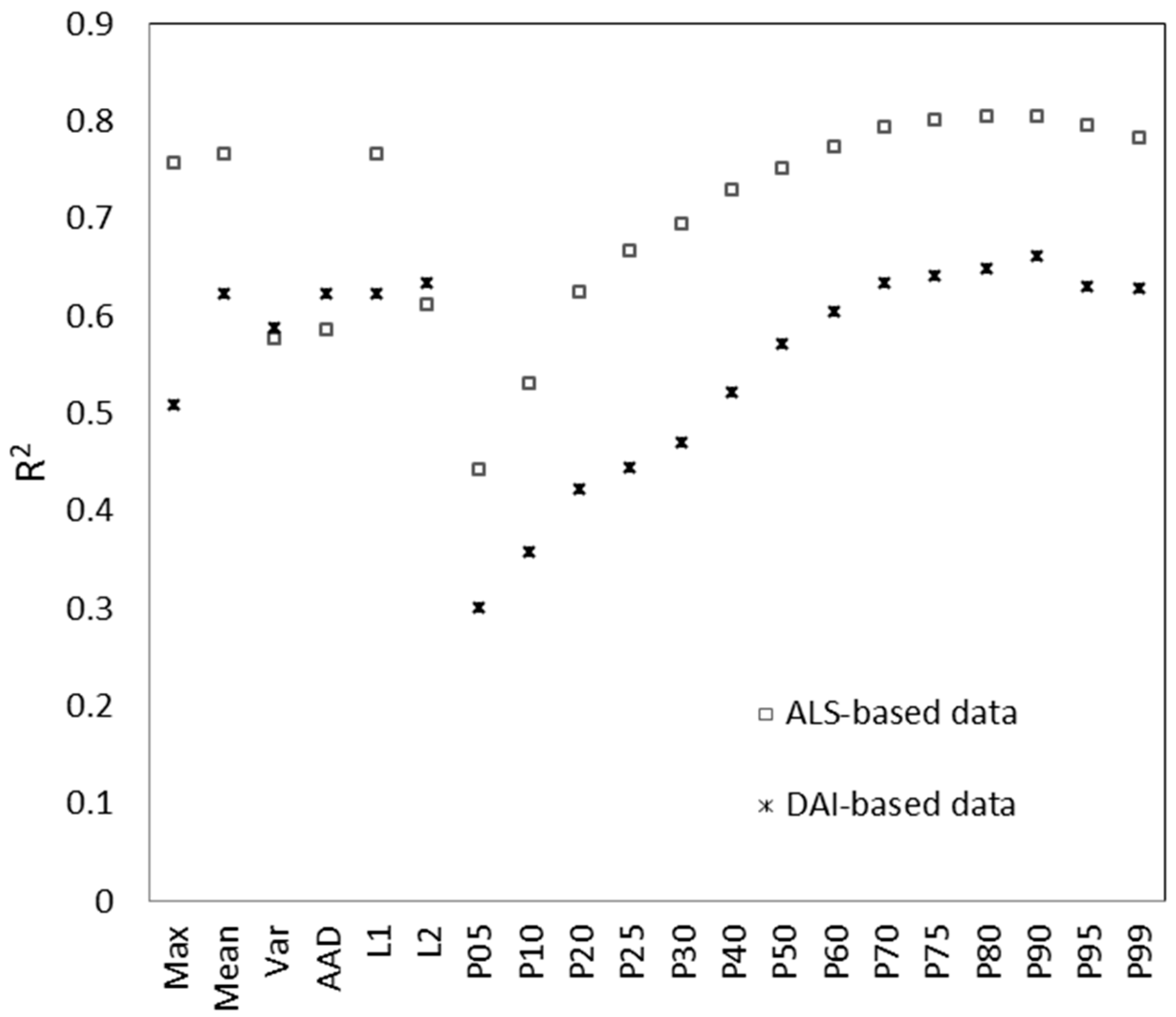
2.3. ALS- and DAI-Based Metrics


| Image acquisition Parameters | Image Processing | ||
|---|---|---|---|
| Images acquired | 552 | Total key point observations | 104,950 |
| Images used | 287 | Total 3D points | 39,636 |
| Mosaic area (ha) | 145.19 | Mean reprojection error (pixels) | 0.7525 |
| * GSD (cm) | 12.74 | ||
| Label | Description |
|---|---|
| Min | Minimum |
| Max | Maximum |
| Mean | Mean |
| SD | Standard deviation |
| Var | Variance |
| CV | Coefficient of variation |
| IQ | Interquartile distance |
| Skew | Skewness |
| Kur | Kurtosis |
| AAD | Average absolute deviation |
| L1, L2, L3, L4 | L-moments (L1, L2, L3, L4) |
| L CV | L-moment coefficient of variation |
| L skew | L-moment skewness |
| L kur | L-moment kurtosis |
| P01…P99 | Percentiles |
2.4. Statistical Model Analysis
3. Results
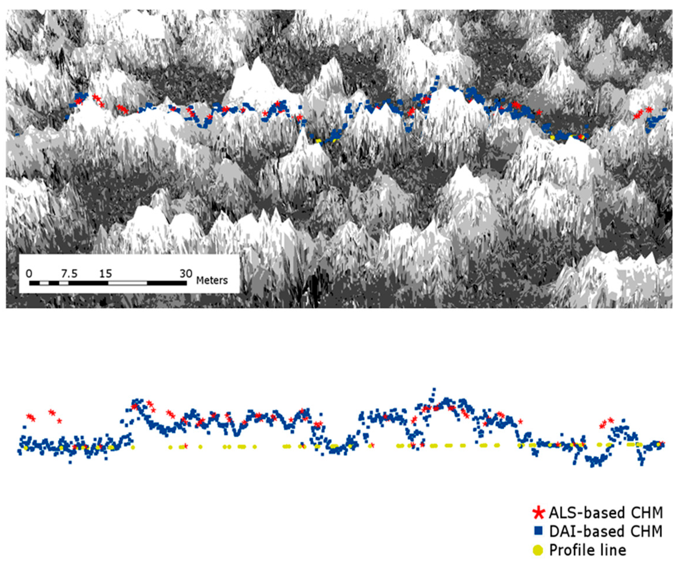
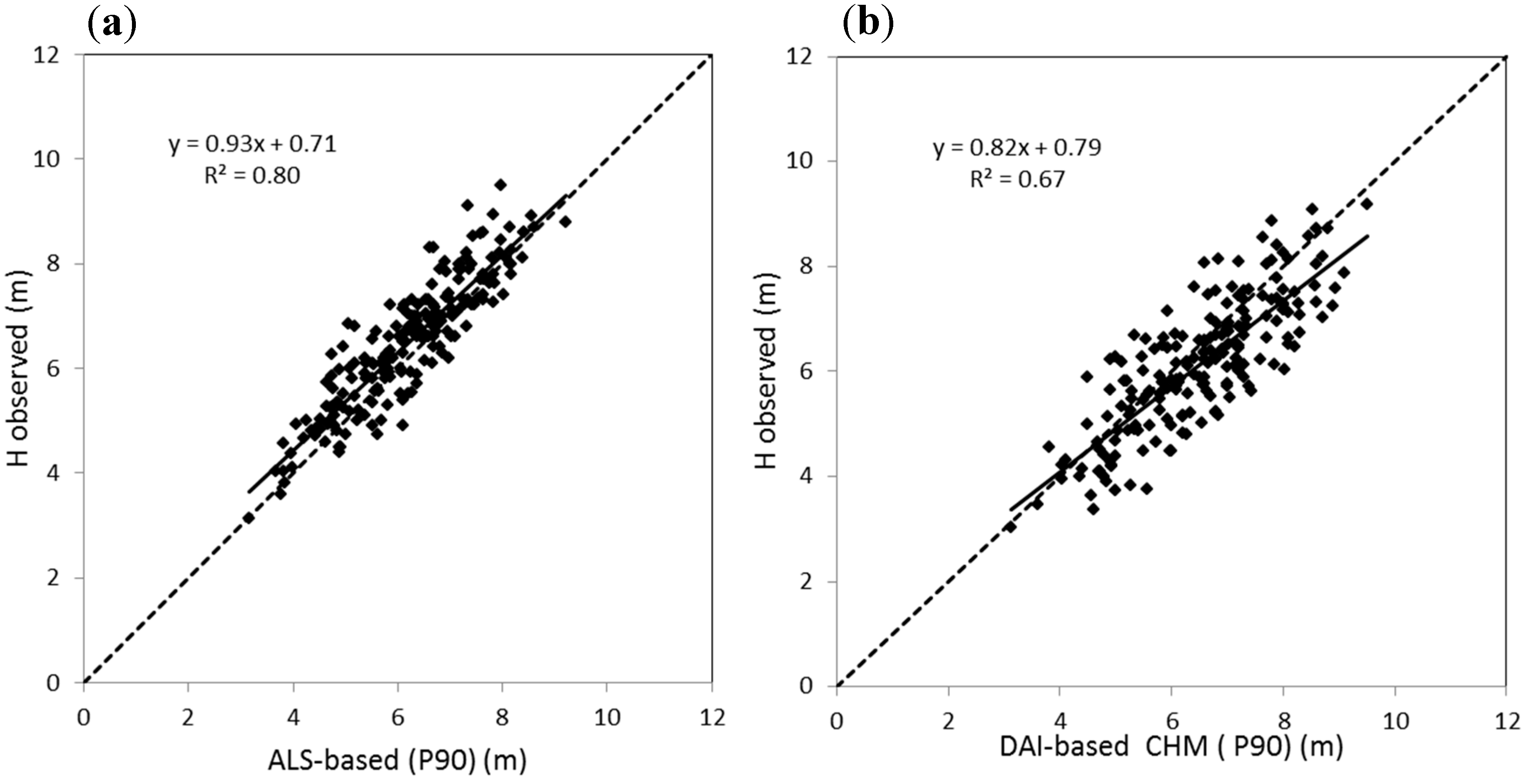
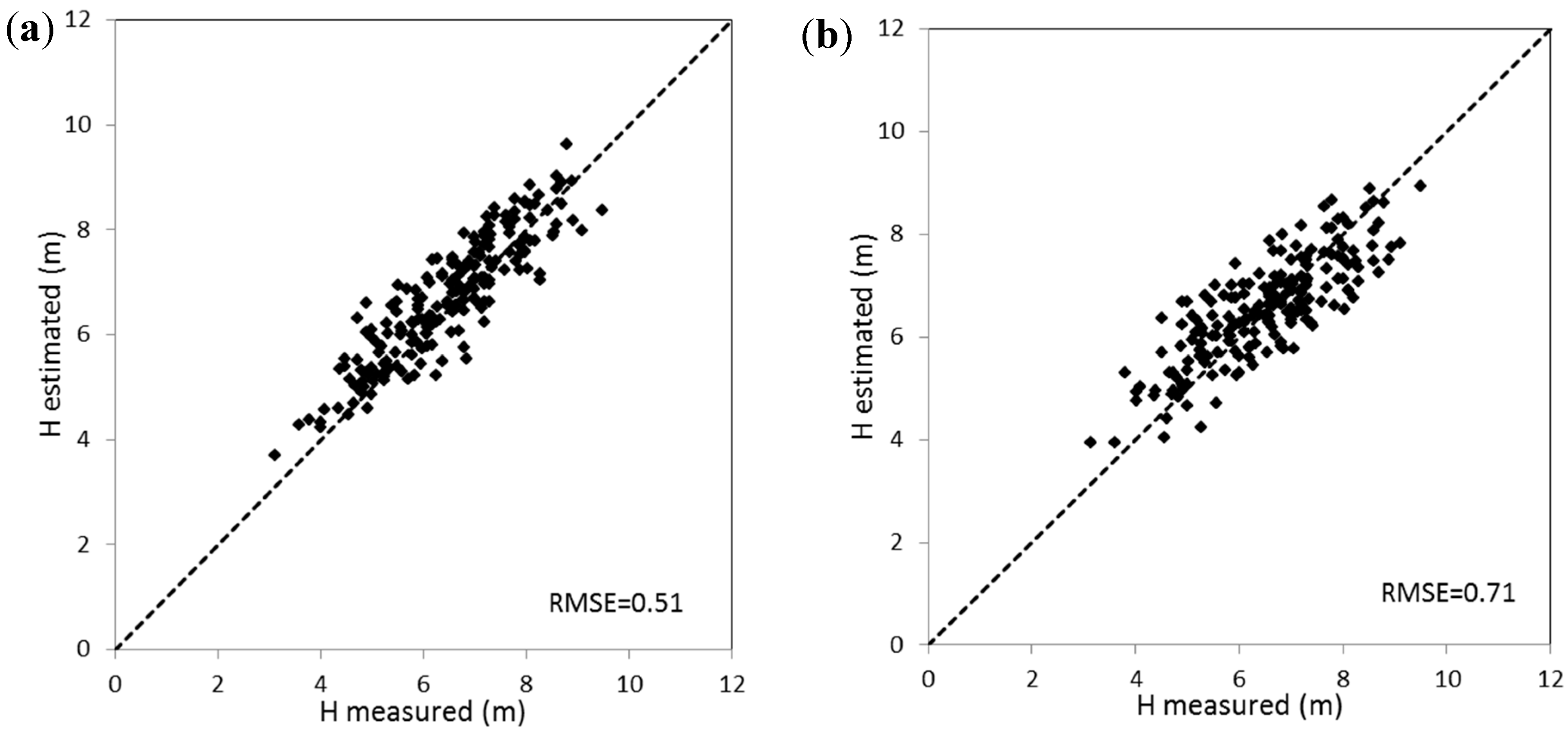
3.1. Canopy Height Estimation from ALS and DAI Data


| Variable | Parameter | Standard Error | t-Value | p > |t| | R2 | |
|---|---|---|---|---|---|---|
| Method | Intercept | 73.69 | 33.13 | 2.22 | <0.01 | |
| DAI-based tree height | P90 | 0.79 | 0.04 | 19.31 | <0.001 | 0.71 |
| Hmin | −35.97 | 16.53 | −2.18 | <0.01 | ||
| Method | Intercept | 0.71 | 0.20 | 3.43 | <0.001 | 0.80 |
| ALS-based tree height | P90 | 0.93 | 0.03 | 28.43 | <0.001 |

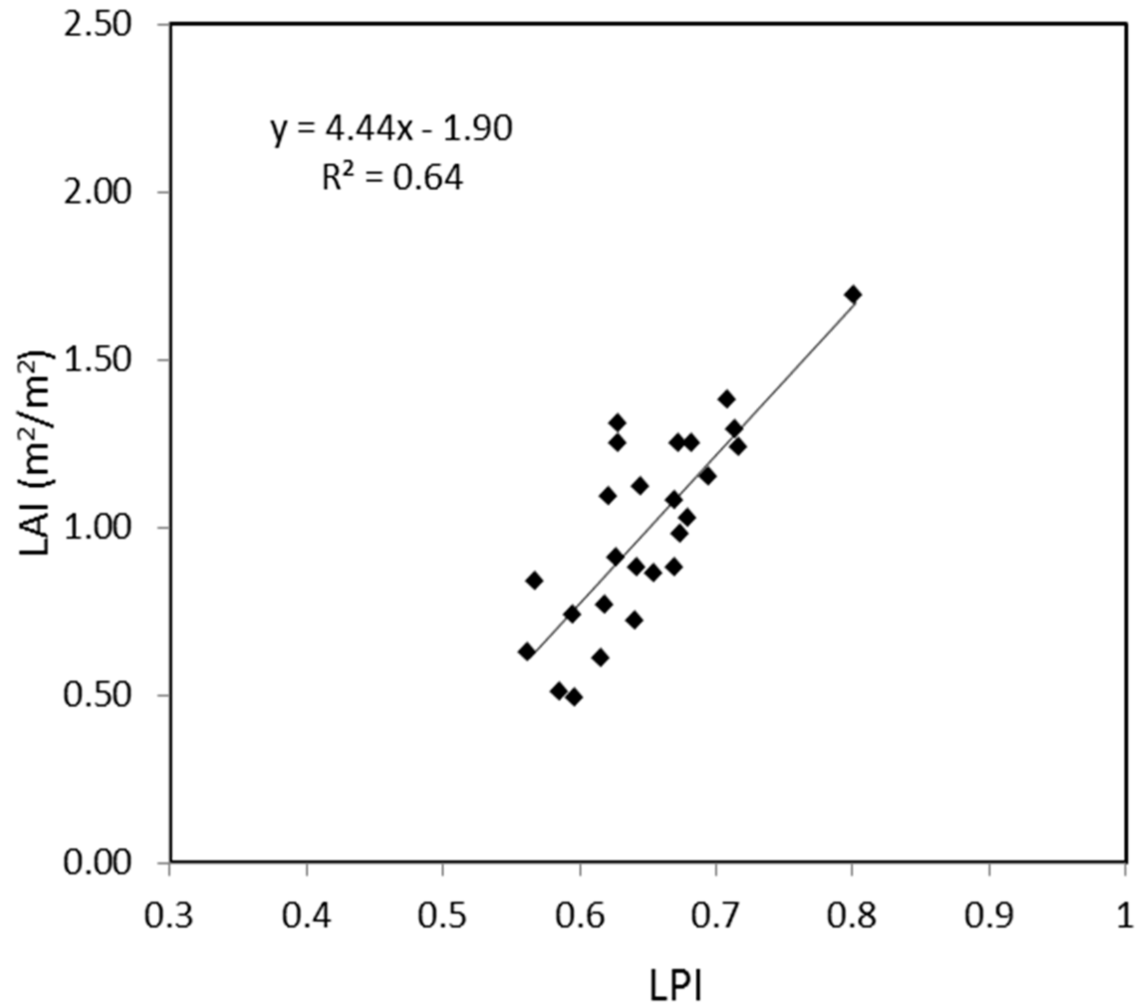
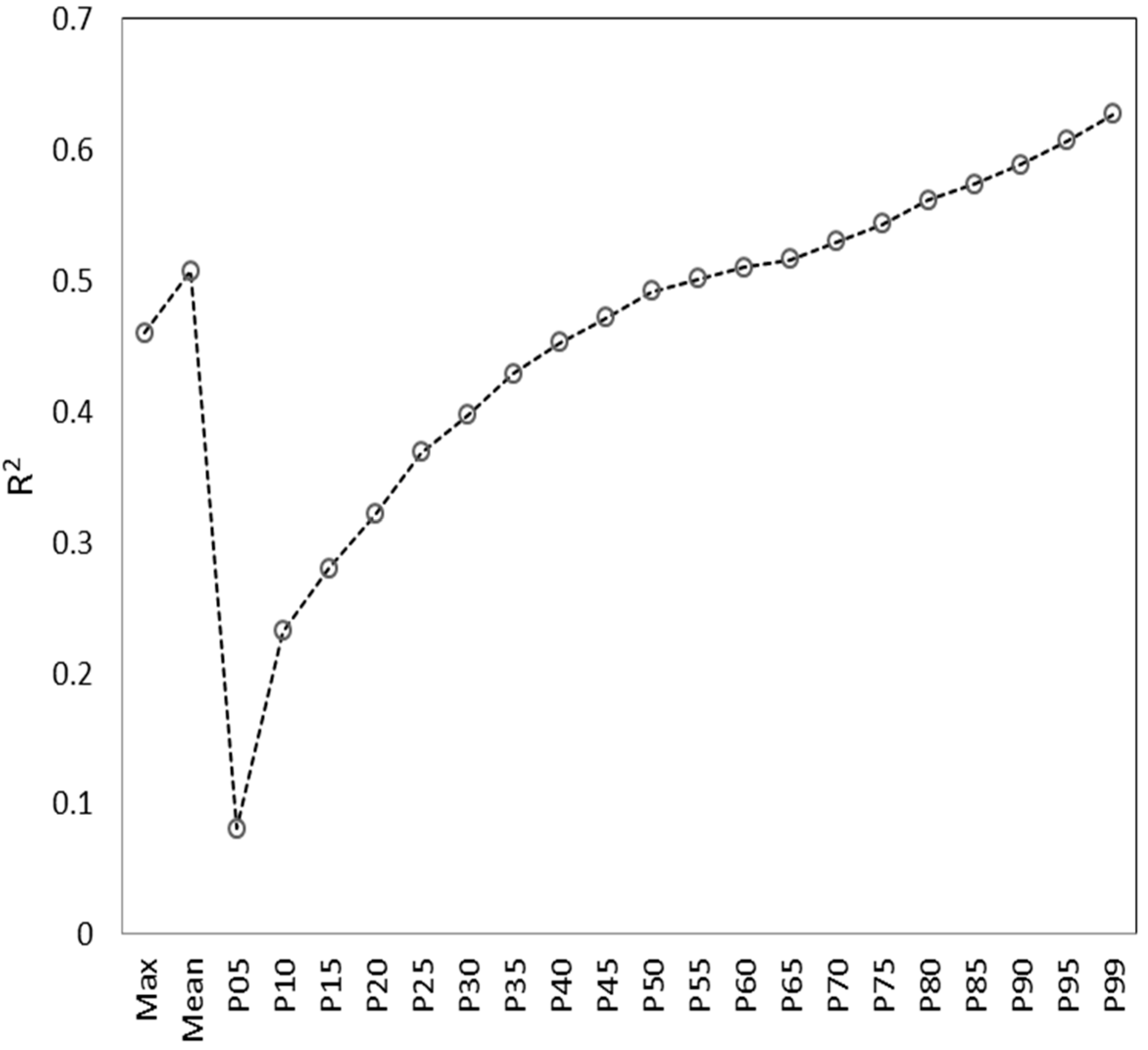
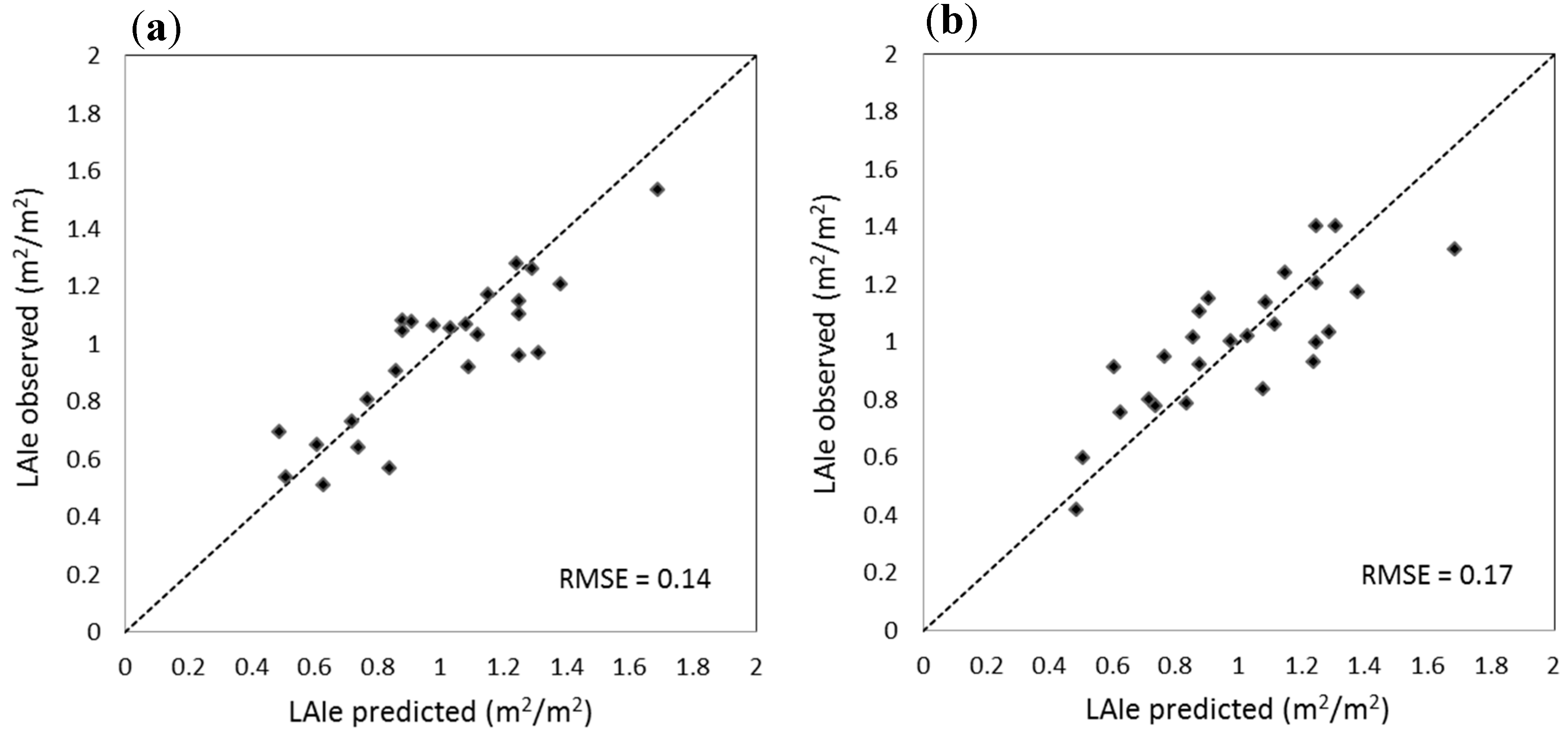
3.2. LAI Estimation from the ALS Data and DAI-Based Canopy Height Model


| Variable | Parameter | Standard Error | t-Value | p > |t| | R2 | |
|---|---|---|---|---|---|---|
| Method | ||||||
| DAI-based LAIe | Intercept | −1.04 | 0.32 | −3.22 | <0.001 | 0.62 |
| P99 DAI NDVI | 9.38 | 1.47 | 6.34 | <0.001 | ||
| Method | ||||||
| ALS-based LAIe | Intercept | −2.65 | 0.77 | 11.63 | <0.001 | 0.75 |
| LPI | 4.78 | 1.01 | 22.38 | <0.001 | ||
| IQ | 0.07 | 0.03 | 4.78 | <0.01 | ||
| P30 | 0.06 | 0.02 | 8.06 | <0.01 |

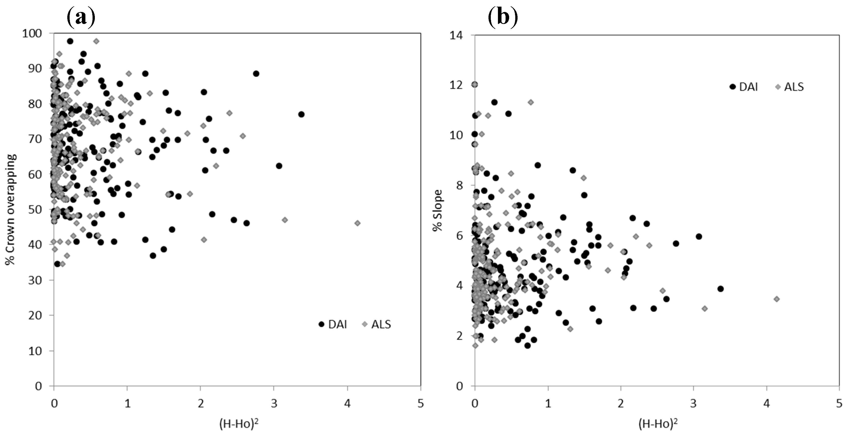
4. Discussion
5. Conclusions
Acknowledgments
Author Contributions
Conflicts of Interest
References
- Breunig, F.M.; Galvão, L.S.; Formaggio, A.R.; Neves Epiphanio, J.C. Directional effects on NDVI and LAI retrievals from MODIS: A case study in Brazil with soybean. Int. J. Appl. Earth Obs. 2011, 13, 34–42. [Google Scholar] [CrossRef]
- Wang, Q.; Adiku, S.; Tenhunen, J.; Granier, A. On the relationship of NDVI with leaf area index in a deciduous forest site. Remote Sens. Environ. 2005, 94, 244–255. [Google Scholar] [CrossRef]
- Birky, A.K. NDVI and a simple model of deciduous forest seasonal dynamics. Ecol. Model. 2001, 143, 43–58. [Google Scholar] [CrossRef]
- Maselli, F. Monitoring forest conditions in a protected mediterranean coastal area by the analysis of multiyear NDVI data. Remote Sens. Environ. 2004, 89, 423–433. [Google Scholar] [CrossRef]
- Heiskanen, J.; Rautiainen, M.; Stenberg, P.; Mõttus, M.; Vesanto, V.-H.; Korhonen, L.; Majasalmi, T. Seasonal variation in MODIS LAI for a boreal forest area in Finland. Remote Sens. Environ. 2012, 126, 104–115. [Google Scholar] [CrossRef]
- Busetto, L.; Michele, M.; Colombo, R. Combining medium and coarse spatial resolution satellite data to improve the estimation of sub-pixel NDVI time series. Remote Sens. Environ. 2008, 112, 118–131. [Google Scholar]
- Tillack, A.; Clasen, A.; Kleinschmit, B.; Förster, M. Estimation of the seasonal leaf area index in an alluvial forest using high-resolution satellite-based vegetation indices. Remote Sens. Environ. 2014, 141, 52–63. [Google Scholar] [CrossRef]
- Darvishzadeh, R.; Atzberger, C.; Skidmore, A.; Schlerf, M. Mapping grassland leaf area index with airborne hyperspectral imagery: A comparison study of statistical approaches and inversion of radiative transfer models. ISPRS J. Photogramm. Remote Sens. 2011, 66, 894–906. [Google Scholar] [CrossRef]
- Morsdorf, F.; Kötz, B.; Meier, E.; Itten, K.I.; Allgöwer, B. Estimation of LAI and fractional cover from small footprint airborne laser scanning data based on gap fraction. Remote Sens. Environ. 2006, 104, 50–61. [Google Scholar] [CrossRef]
- Lee, A.C.; Lucas, R.M. A LiDAR-derived canopy density model for tree stem and crown mapping in Australian forests. Remote Sens. Environ. 2007, 111, 493–518. [Google Scholar] [CrossRef]
- Zhao, F.; Strahler, A.H.; Schaaf, C.L.; Yao, T.; Yang, X.; Wang, Z.; Schull, M.A.; Román, M.O.; Woodcock, C.E.; Olofsson, P.; et al. Measuring gap fraction, element clumping index and LAI in sierra forest stands using a full-waveform ground-based lidar. Remote Sens. Environ. 2012, 125, 73–79. [Google Scholar] [CrossRef]
- Solberg, S.; Næsset, E.; Hanssen, K.H.; Christiansen, E. Mapping defoliation during a severe insect attack on Scots pine using airborne laser scanning. Remote Sens. Environ. 2006, 102, 364–376. [Google Scholar] [CrossRef]
- Zhao, K.; Popescu, S. Lidar-based mapping of leaf area index and its use for validating GLOBCARBON satellite LAI product in a temperate forest of the southern USA. Remote Sens. Environ. 2009, 113, 1628–1645. [Google Scholar] [CrossRef]
- Hall, S.A.; Burke, I.C.; Box, D.O.; Kaufmann, M.R.; Stoker, J.M. Estimating stand structure using discrete-return lidar: An example from low density, fire prone ponderosa pine forests. For. Ecol. Manage. 2005, 208, 189–209. [Google Scholar] [CrossRef]
- Næsset, E.; Bjerknes, K.-O. Estimating tree heights and number of stems in young forest stands using airborne laser scanner data. Remote Sens. Environ. 2001, 78, 328–340. [Google Scholar] [CrossRef]
- Treitz, P.; Lim, K.; Woods, M.; Pitt, D.; Nesbitt, D.; Etheridge, D. LiDAR sampling intensity for forest resource inventories in Ontario, Canada. Remote Sens. 2012, 4, 830–848. [Google Scholar] [CrossRef]
- Næsset, E. Determination of mean tree height of forest stands by means of digital photogrammetry. Scand. J. For. Res. 2002, 17, 446–459. [Google Scholar] [CrossRef]
- Næsset, E. Predicting forest stand characteristics with airborne scanning laser using a practical two-stage procedure and field data. Remote Sens. Environ. 2002, 80, 88–99. [Google Scholar] [CrossRef]
- Holmgren, J.; Nilsson, M.; Olsson, H. Simulating the effects of LiDAR scanning angle for estimation of mean tree height and canopy closure. Can. J. Remote Sens. 2003, 29, 623–632. [Google Scholar] [CrossRef]
- González-ferreiro, E.; Diéguez-aranda, U.; Miranda, D. Estimation of stand variables in Pinus radiata D. Don plantations using different LiDAR pulse densities. Forestry 2012, 85, 281–292. [Google Scholar] [CrossRef]
- Magnusson, M.; Fransson, J.E.S.; Holmgren, J. Effects of estimation accuracy of forest variables using different pulse density of laser data. For. Sci. 2010, 53, 619–626. [Google Scholar]
- Popescu, S.C.; Wynne, R.H. Seeing the trees in the forest: using LiDAR and multispectral data fusion with local filtering and variable window size for estimating tree height. Photogramm. Eng. Remote Sens. 2004, 70, 589–604. [Google Scholar] [CrossRef]
- Yu, X.; Hyyppä, J.; Kaartinen, H.; Maltamo, M. Automatic detection of harvested trees and determination of forest growth using airborne laser scanning. Remote Sens. Environ. 2004, 90, 451–462. [Google Scholar] [CrossRef]
- Popescu, S.C.; Wynne, R.H.; Nelson, R.H. Measuring individual tree crown diameter with LiDAR and assessing its influence on estimating forest volume and biomass. Can. J. Remote Sens. 2003, 29, 564–577. [Google Scholar] [CrossRef]
- Popescu, S.C.; Kaiguang, Z. A voxel-based LiDAR method for estimating crown base height for deciduous and pine trees. Remote Sens. Environ. 2008, 112, 767–781. [Google Scholar] [CrossRef]
- Hyyppä, J.; Inkinen, M. Detecting and estimating attributes for single trees using laser scanner. Photogramm. J. Finl. 1999, 16, 27–42. [Google Scholar]
- Vauhkonen, J.; Tokola, T.; Packalén, P.; Maltamo, M. Identification of Scandinavian commercial species of individual trees from airborne laser scanning data using alpha shape metrics. For. Sci. 2009, 55, 37–47. [Google Scholar]
- Järnstedt, J.; Pekkarinen, A.; Tuominen, S.; Ginzler, C.; Holopainen, M.; Viitala, R. Forest variable estimation using a high-resolution digital surface model. ISPRS J. Photogramm. Remote Sens. 2012, 74, 78–84. [Google Scholar] [CrossRef]
- Dandois, J.P.; Ellis, E.C. High spatial resolution three-dimensional mapping of vegetation spectral dynamics using computer vision. Remote Sens. Environ. 2013, 136, 259–276. [Google Scholar] [CrossRef]
- Berni, J.A.J.; Zarco-Tejada, P.J.; Suarez, L.; Fereres, E. Thermal and narrow-band multispectral remote sensing for vegetation monitoring from an unmanned aerial vehicle. IEEE Trans. Geosci. Remote Sens. 2009, 47, 722–738. [Google Scholar] [CrossRef]
- Haala, N.; Hastedt, H.; Wolf, K.; Ressl, C.; Baltrusch, S. Digital photogrammetric camera evaluation—Generation of digital elevation models. Photogramm.-Fernerkund.-Geoinf. 2010, 2, 98–15. [Google Scholar]
- Baltsavias, E.; Gruen, A.; Eisenbeiss, H.; Zhang, L.; Waser, L.T. High quality image matching and automated generation of 3D tree models. Int. J. Remote Sens. 2008, 29, 1243–1259. [Google Scholar] [CrossRef]
- St-Onge, B.; Hu, Y.; Véga, C. Mapping the height and above-ground biomass of a mixed forest using LiDAR and stereo Ikonos images. Int. J. Remote Sen. 2007, 29, 1277–1294. [Google Scholar] [CrossRef]
- Valbuena, R. Integrating airborne laser scanning with data from global navigation satellite systems and optical sensors. Manag. For. Ecos. 2014, 27, 63–88. [Google Scholar]
- Zarco-Tejada, P.J.; Diaz-Varela, R.; Angileri, V.; Loudjani, P. Tree height quantification using very high resolution imagery acquired from an unmanned aerial vehicle (UAV) and automatic 3D photo reconstruction methods. Eur. J. Agron. 2014, 55, 89–99. [Google Scholar] [CrossRef]
- Moralejo, E.; García Muñoz, J.A.; Descals, E. Susceptibility of Iberian trees to Phytophthora ramorum and P. cinnamomi. Plant pathol. 2009, 58, 271–283. [Google Scholar] [CrossRef]
- Baatz, M.; Schäpe, A. Multiresolution segmentation: An optimization approach for high quality multi-scale image segmentation. In Proceedings of Angewandte Geographische Informationsverarbeitung XII; Beiträge zum AGIT-Symposium Salzburg 2000. Herbert Wichmann Verlag: Karlsruhe, Germany, 2000; pp. 12–23. [Google Scholar]
- Axelsson, P. DEM generation from laser scanner data using adaptive TIN models. Int. Arch. Photogramm. Remote Sens. 2000, 33, 110–117. [Google Scholar]
- McGauhey, R.J. FUSION/LDV: Software for LiDAR Data Analysis and Visualization; USDA Forest Service, Pacific Northwest Research Station: Seattle, WA, USA, 2009. [Google Scholar]
- Curran, P.J.; Atkinson, P.M. Geostatistics and remote sensing. Prog. Phys. Geogr. 1998, 22, 61–78. [Google Scholar] [CrossRef]
- Freund, R.J.; Littell, R.C. SAS System for Regression; SAS Institute Inc.: Cary, NC, USA, 1986. [Google Scholar]
- Belsley, D.A. A guide to using the collinearity diagnostics. Comput. Sci. Econ. Manage. 1991, 4, 33–50. [Google Scholar]
- Korpela, I.; Anttila, P. Appraisal of the mean height of trees by means of image matching of digitised aerial photographs. Photogramm. J. Finl. 2004, 19, 23–36. [Google Scholar]
- Bohlin, J.; Wallerman, J.; Fransson, J.E.S. Forest variable estimation using photogrammetric matching of digital aerial images in combination with a high-resolution DEM. Scand. J. For. Res. 2012, 27, 692–699. [Google Scholar] [CrossRef]
- Breidenbach, J.; Astrup, R. Small area estimation of forest attributes in the Norwegian National Forest Inventory. Eur. J. For. Res. 2012, 131, 1255–1267. [Google Scholar] [CrossRef]
- Persson, A.; Holmgren, J.; Söerman, U. Detecting and measuring individual trees using an airborne laser scanner. Photogramm. Eng. Remote Sens. 2002, 68, 925–932. [Google Scholar]
- Feikema, P.M.; Morris, J.D.; Beverly, C.R.; Collopy, J.J.; Baker, T.G.; Lane, P.N.J. Validation of plantation transpiration in south-eastern Australia estimated using the 3PG+ forest growth model. For. Ecol. Manage. 2010, 260, 663–678. [Google Scholar] [CrossRef]
- Wang, Z.; Grant, R.F.; Arain, M.A.; Chen, B.N.; Coops, N.; Hember, R.; Kurz, W.A. Evaluating weather effects on interannual variation in net ecosystem productivity of a coastal temperate forest landscape: A model intercomparison. Ecol. Model. 2011, 222, 3236–3249. [Google Scholar] [CrossRef]
- Zhou, X.; Peng, C.; Dang, Q.L.; Chen, J.; Parton, S. Predicting forest growth and yield in northeastern Ontario using the process-based model of TRIPLEX1.0. Can. J. For. Res. 2005, 35, 2268–2280. [Google Scholar] [CrossRef]
© 2014 by the authors; licensee MDPI, Basel, Switzerland. This article is an open access article distributed under the terms and conditions of the Creative Commons Attribution license (http://creativecommons.org/licenses/by/4.0/).
Share and Cite
Hernández-Clemente, R.; Navarro-Cerrillo, R.M.; Ramírez, F.J.R.; Hornero, A.; Zarco-Tejada, P.J. A Novel Methodology to Estimate Single-Tree Biophysical Parameters from 3D Digital Imagery Compared to Aerial Laser Scanner Data. Remote Sens. 2014, 6, 11627-11648. https://doi.org/10.3390/rs61111627
Hernández-Clemente R, Navarro-Cerrillo RM, Ramírez FJR, Hornero A, Zarco-Tejada PJ. A Novel Methodology to Estimate Single-Tree Biophysical Parameters from 3D Digital Imagery Compared to Aerial Laser Scanner Data. Remote Sensing. 2014; 6(11):11627-11648. https://doi.org/10.3390/rs61111627
Chicago/Turabian StyleHernández-Clemente, Rocío, Rafael M. Navarro-Cerrillo, Francisco J. Romero Ramírez, Alberto Hornero, and Pablo J. Zarco-Tejada. 2014. "A Novel Methodology to Estimate Single-Tree Biophysical Parameters from 3D Digital Imagery Compared to Aerial Laser Scanner Data" Remote Sensing 6, no. 11: 11627-11648. https://doi.org/10.3390/rs61111627