Using Tree Detection Algorithms to Predict Stand Sapwood Area, Basal Area and Stocking Density in Eucalyptus regnans Forest

Abstract

Managers of forested water supply catchments require efficient and accurate methods to quantify changes in forest water use due to changes in forest structure and density after disturbance. Using Light Detection and Ranging (LiDAR) data with as few as 0.9 pulses m⁻², we applied a local maximum filtering (LMF) method and normalised cut (NCut) algorithm to predict stocking density (S_Den) of a 69-year-old Eucalyptus regnans forest comprising 251 plots with resolution of the order of 0.04 ha. Using the NCut method we predicted basal area (BA_Ha) per hectare and sapwood area (SA_Ha) per hectare, a well-established proxy for transpiration. Sapwood area was also indirectly estimated with allometric relationships dependent on LiDAR derived S_Den and BA_Ha using a computationally efficient procedure. The individual tree detection (ITD) rates for the LMF and NCut methods respectively had 72% and 68% of stems correctly identified, 25% and 20% of stems missed, and 2% and 12% of stems over-segmented. The significantly higher computational requirement of the NCut algorithm makes the LMF method more suitable for predicting S_Den across large forested areas. Using NCut derived ITD segments, observed versus predicted stand BA_Ha had R² ranging from 0.70 to 0.98 across six catchments, whereas a generalised parsimonious model applied to all sites used the portion of hits greater than 37 m in height (PH₃₇) to explain 68% of BA_Ha. For extrapolating one ha resolution SA_Ha estimates across large forested catchments, we found that directly relating SA_Ha to NCut derived LiDAR indices (R² = 0.56) was slightly more accurate but computationally more demanding than indirect estimates of SA_Ha using allometric relationships consisting of BA_Ha (R² = 0.50) or a sapwood perimeter index, defined as (BA_HaS_Den)^½ (R² = 0.48).

1. Introduction

Many benefits of forests are strongly influenced by forest structure and density. For example, forest regeneration after timber harvesting or wildfire affects forest structure and density, which can have dramatic effects on forest hydrology, forest growth rates, carbon stores and wildlife habitat. Advancements in Light Detection and Ranging (LiDAR) sensors are providing opportunity for detailed analysis of forest structure and density at unprecedented spatial scales. At landscape spatial scales, LiDAR data are being collected from forests across the world with fine scale information on individual trees and stand structure. New algorithms for analysing these large datasets are being developed and applied to produce information useful for forest management, particularly in the boreal forests of the northern hemisphere [1].

In south-eastern Australia, wildfires have burnt approximately 3 million hectares of forested land since 2003, and in addition, intensive forest harvesting in recent decades has stimulated large-scale changes in forest age. In tall eucalypt forests, replacing old forest with young healthy regenerating forest leads to an overall decline in catchment water yields over the forest regeneration period [2,3,4,5]. Understanding and managing water security in Australia depends critically on the availability of efficient methods for quantifying the relationship between forest water use and changes in forest structure and density over the post-disturbance regeneration period.

Characterising forests with LiDAR data is commonly done on two spatial scales: (i) area based, where the biophysical variables are averaged over an area encompassing several trees; and (ii) tree based, where individual tree dimensions are estimated using individual tree detection (ITD) algorithms. In ecohydrology research, forest transpiration (T) is commonly derived from tree-scale measurements of sapwood area (SA_1.3) at 1.3 m, and therefore using ITD algorithms to characterise biophysical properties of forests at the individual tree-scale may prove useful for scaling T from a tree-to-landscape level.

Compared to LiDAR research in boreal forests (see [1] for review), relatively few studies have published LiDAR based estimates of forest biophysical properties in eucalypt forests of Australia. Haywood and Sutton [6] estimated plot-level basal area per hectare (BA_Ha) in Eucalyptus regnans forests of south eastern Australia using simple predictor variables such as height percentiles and summary statistics of the vertical vegetation profile (r² = 0.56; RMSE = 14.7 m²). Jaskierniak et al. [7] characterised a multilayered E. regnans forest structure using mixture distribution functions to predict plot-level BA_Ha with r² ranging from 0.6 to 0.89 in 18, 37 and 70 year old stands. In mixed species eucalyptus forests (MSEF), [8] derived plot level LiDAR indices using a Weibull distribution function, height percentiles, and summary statistics to predict stand BA_Ha and sapwood area per hectare (SA_Ha) with r² of 0.88 and 0.7 respectively.

Kaartinen et al. [9,10] provide a comprehensive review of ITD methods, all of which have been applied in the northern hemisphere. Kaartinen and Hyyppa [11] evaluated the quality, accuracy and feasibility of ITD methods in boreal forests and reported large variation in the quality of published methods with varying laser point densities. It has been shown that ITD performs best with laser scanning density of 5–10 pulses·m⁻², which is higher than the 0.9 and 4 pulses·m⁻² available over our study sites. Several studies undertaken in Scandinavian and European forests have demonstrated that it is possible to detect 40%–70% of all trees using an ITD approach [12,13]. In deciduous forests, the complex crown shape and structure results in generally lower success rates [14,15]. In North American forests, success rates have been largely dependent on canopy density [16]. Persson et al. [12,17] used the same ITD algorithm and managed detection rates of 71% for Scandinavian forest dominated by spruce and pine, 51% for coniferous forests, 45% for Bavarian Forest National Park, and 40% for deciduous forests. These studies suggest that ITD rates are highly dependent on forest structure. To our knowledge, we demonstrate for the first time the potential use of ITD methods in native eucalypt forests, which represent a forest structure substantially different to those of previous studies.

Most ITD algorithms generate canopy height models (CHM) to locate local height maxima in LiDAR data, which are then considered representative of the stem positions within the forest [18,19,20]. Using this approach, point clouds are typically segmented into crown diameters using watershed algorithms [21], slope-based segmentation methods [12], or gridded methods smoothed with Gaussian filters [20]. More advanced ITD methods recognise that heterogeneous multilayered forests, such as E. regnans forests in our study, require a 3D approach to address the segmentation problem [22,23,24]. In E. regnans forest, an ITD algorithm needs to be robust enough to differentiate different vegetation strata down the vertical profile, whilst accurately handling different sized overstorey crowns across a heterogeneous forest landscape.

The overarching aim of our project is to acquire an accurate and robust measure of spatial variability in T per hectare across Melbourne’s forested water catchments. This required us to develop a methodology that uses LiDAR indices to estimate SA_Ha, a well-established proxy for T. Our research was conducted in forested catchments supplying approximately 90% of the water used by the city of Melbourne. Considering Melbourne’s water catchments consist of approximately 155,000 ha of forested land, predicting tree-specific SA_1.3 across the landscape is not strictly required by the water management agency—a relationship between plot-level LiDAR indices and SA_Ha is sufficient for water yield assessment purposes. We argue that a more robust and accurate relationship between plot-level LiDAR indices and field measured SA_Ha will eventuate if an ITD algorithm removes within-plot LiDAR points that represent trees outside the plot, and includes LiDAR points outside of plots if they represent measured trees within-plots. To confirm this, we compare our ITD derived BA_Ha estimates to those of [7] who characterised the forest structure across five of the same permanent plot catchments using an area-based mixture distribution function method.

To the authors’ knowledge, [8] is the only study that has used LiDAR to capture within catchment variation in SA_Ha and demonstrated that forest heterogeneity across an elevation gradient was associated with a threefold change in annual T. They applied a SA_1.3/BA_1.3 relationship (R_1.3) to predict plot-level SA_Ha from plot-level BA_1.3 measurements_, and regressed the SA_Ha estimate against explanatory variables derived from LiDAR data to spatially extrapolate SA_Ha across two catchments (136 ha and 87 ha).

Adopting this approach requires the assumption that R_1.3 is constant across Melbourne’s water catchments. Recently, [25] have shown high spatial variability in R_1.3 and the SA_Ha/BA_Ha relationship (R_Ha) across the landscape, and provide a more consistent species-specific relationship observed between SA_Ha and an index of total sapwood perimeter per hectare, defined as $\sqrt{ B{A}_{Ha}{S}_{Den}}$, where S_Den is stocking density of overstorey trees per hectare. In order to determine how well LIDAR may estimate $\sqrt{ B{A}_{Ha}{S}_{Den}},$ we evaluate our ability to predict BA_Ha and S_Den across all sites. We also measured SA_1.3 across an intensively studied 5 ha site in order to determine how well the perimeter index may be used to scale tree-level SA_1.3 to a stand- and landscape-level using LiDAR data. The following questions are addressed in the present study:

• Can LiDAR data with less than 1 pulse per m² identify individual trees within a dense E. regnans forest, and if so what is the ITD rate?
• Can ITD methods improve predictions of stand BA_Ha in E. regnans forests compared to previous area based methods applied to the same sites?
• Is it more accurate to predict stand SA_Ha with: (i) a R_Ha relationship and BA_Ha estimates derived from LiDAR; (ii) a stand perimeter index that relies on accurate S_Den and BA_Ha estimates; or (iii) LiDAR indices directly related to stand SA_Ha?

2. Materials and Methods

2.1. Site Description and Processing of Field Measurements

2.1.1. Harvested 5 Hectare Forest

A complete inventory of overstorey SA_1.3 and BA_1.3 was mapped over a 5 ha harvested site located along the upper reaches of the Great Dividing Range in Toolangi State Forest, approximately 80 km northeast of Melbourne, Australia. Refer to [26] for a detailed description of the site’s topography, climate, and soil conditions. The overstorey consists of a pure E. regnans forest stand, originated from an even-aged regeneration caused by a wildfire in 1939, and the regrowth was harvested in the summer of December 2011 (73 years old). We estimated SA_1.3 and BA_1.3 for all stems across the site with measured stump dimensions data consisting of stump height (H_S), diameter at stump height (D_S), and diameter 20 cm below stump height (D_S20), as well as photo images of stump cross-sections collected two months after harvest in order to differentiate sapwood from heartwood. Sapwood area and BA at stump height (SA_S and BA_S respectively) were calculated by correcting for lens distortion in each stump’s cross-sectional image, and then scaling the images to actual cross-sectional area. As described by [26], a mixed effects model was then used to predict SA_1.3 and BA_1.3 by coupling SA_S and BA_S estimates with stump dimensions data, and tree and sapwood taper data.

Table 1 provides diameter distributions of overstorey trees across all sites (see Section 2.1.2 for description of other sites), and shows the 5 ha site had highly variable S_Den and BA_Ha suitable for calibrating both ITD algorithms. To apply the ITD algorithms, each stump’s position was accurately located using a 2 cm resolution orthophoto mosaic of the site after the post-harvest burn. To generate the orthophoto mosaic, images collected using a UAV platform (multi-rotor OktoKopter) were georectified following [25,27]. In brief the method applied a photogrammetric technique called structure from motion (SfM) to orientate individual images and generate a dense point cloud with aerial triangulation. The generated point cloud was used to geometrically correct and mosaic the individual images. A detailed outline of the UAV platform’s specifications and post-processing procedure are outlined in [25].

Table 1. Summary statistics of sites exposed to a range of silviculture treatments.

Catchment	Size (m2)	Treatment	Plot #	Eucalyptus Tree Count per Hectare				Eucalyptus Basal Area per Hectare
				Min	Std Dev	Mean	Max	Min	Std Dev	Mean	Max
BS 1	15 × 20	Patch cut 54%	76	0	85	118	266	0	34	36	123
BS 2	40 × 40	Thinned 33%	7	75	20	96	131	34	8	48	59
BS 3	40 × 40	Thinned 50%	7	50	21	76	112	36	8	48	63
ET2	15 × 40	Removed Understorey	21	0	19	133	217	0	61	43	67
ET3	15 × 40	No Treatment	40	17	65	140	317	15	16	51	84
5Ha	20 × 20	No Treatment	100	25	63	160	300	8	17	51	96

Note: Catchments are abbreviated as follows: Black Spur 1 (BS 1), Black Spur 2 (BS2), Black Spur 3 (BS3), Ettercon 2 (ET2), Ettercon 3 (ET3), and the 5 ha harvest site (5Ha).

Table 1. Summary statistics of sites exposed to a range of silviculture treatments.

Catchment	Size (m2)	Treatment	Plot #	Eucalyptus Tree Count per Hectare				Eucalyptus Basal Area per Hectare
				Min	Std Dev	Mean	Max	Min	Std Dev	Mean	Max
BS 1	15 × 20	Patch cut 54%	76	0	85	118	266	0	34	36	123
BS 2	40 × 40	Thinned 33%	7	75	20	96	131	34	8	48	59
BS 3	40 × 40	Thinned 50%	7	50	21	76	112	36	8	48	63
ET2	15 × 40	Removed Understorey	21	0	19	133	217	0	61	43	67
ET3	15 × 40	No Treatment	40	17	65	140	317	15	16	51	84
5Ha	20 × 20	No Treatment	100	25	63	160	300	8	17	51	96

Note: Catchments are abbreviated as follows: Black Spur 1 (BS 1), Black Spur 2 (BS2), Black Spur 3 (BS3), Ettercon 2 (ET2), Ettercon 3 (ET3), and the 5 ha harvest site (5Ha).

2.1.2. Forest Hydrology Research Catchments

Data from the long-term forest hydrology research catchments includes five catchments with 151 permanent growth plots consisting of 1939 wildfire E. regnans regrowth. The catchments were treated in the 1970s to investigate the impact of forest density and age on forest water use. Treatments across the catchments consisted of: selective forest thinning with 50% and 33% BA removal; removal of understorey only; and patch cut removing 54% of the area with clear fell harvesting. The permanent plots were revisited in the summer of September 2008 for measurement of diameter at breast height over bark (DBHOB) of all eucalyptus trees. Exact tree locations within plots were not mapped, and instead trees were allocated into 5 m × 5 m sub-plots. Table 1 provide summary statistics indicating a diverse range of forest conditions across the sites.

2.1.3. LiDAR Data

The LiDAR data were acquired in 2007 and 2008 for the 5 ha site and permanent plot sites respectively. Table 2 provides the flight details and sensor configurations for both flights. Data acquisition over the 5 ha site consisted of 0.9 pulses·m⁻² as the flight covered an area encompassing approximately 500,000 ha of the Central Highlands Forest Management Area, whereas the flight over the research catchments was limited to the study site and consisted of 4 pulses·m⁻². In both cases, the LiDAR point cloud was measured relative to sea level and needed to be converted into height above ground in order to represent the vegetation height. For this purpose, the ground was classified with an iterative procedure that built a triangulated model of the ground surface [27,28]. All ground classified points were then applied to a thin-plate spline interpolator, using the ANUDEM algorithm [29], to produce a digital terrain model (DTM). The DTM was subtracted from the height of the LiDAR points to produce a point cloud representing the vegetation height.

Overlapping LiDAR flight paths may distort the density of points when some sites are represented by one flight path and others by two overlapping flight paths. To address this problem, a point density map identified strips of overlapping paths, which were delineated and intersected down the middle to define the boundary used to adjoin adjacent flight paths. The dataset’s GPS timestamp was then used to segregate the LIDAR into flight paths in order to remove any overlap.

Table 2. Flight details and sensor configuration for the two LiDAR data acquisition flights.

LiDAR System Configurations	Permanent Plots	5 ha Site
Date of flight	26 August 2007	19 November 2007 To 10 January 2008
Sensor type	Optech ALTM3100	ALTM3100EA
Scan angle (degrees)	28	NA
Pulse repetition rate (kHz)	100	71
Mean footprint size (m)	0.16	0.26
Pulses per square metre	4	0.90
Maximum returned signals	4	4

Table 2. Flight details and sensor configuration for the two LiDAR data acquisition flights.

LiDAR System Configurations	Permanent Plots	5 ha Site
Date of flight	26 August 2007	19 November 2007 To 10 January 2008
Sensor type	Optech ALTM3100	ALTM3100EA
Scan angle (degrees)	28	NA
Pulse repetition rate (kHz)	100	71
Mean footprint size (m)	0.16	0.26
Pulses per square metre	4	0.90
Maximum returned signals	4	4

2.2. Individual Tree Detection Procedure

2.2.1. Normalised Cut Segmentation

Individual tree segments are derived using the normalised cut (NCut) method known from image segmentation [30] and developed for LIDAR applications by [23]. The NCut method was used to identify overstorey tree segments in LiDAR data, which were used to estimate S_Den and BA_Ha across all sites and SA_Ha across the 5 ha site. The procedure first subdivides the region of interest (ROI) into a voxel structure with $N_v=N_v^x+ N_v^y+ N_v^z$ voxels and a voxel space (vp) of 1 m [23]. The LiDAR points are assigned to voxels (l, m, n) (l =1, ..., $N_v^x$; m=1, ..., $N_v^y$; n =1, ..., $N_v^z$) of size vp³ and only voxels with at least one point are used in the segmentation procedure. The reduced voxel space is then represented as a weighted undirected graph G = (V, E), where V is a set of nodes, one for each voxel, and E is a set of edges formed between each pair of nodes. The edges are weighted to represent the affinity between connected nodes, and the weight function w_ij is defined as [23]:

$$w_{ij}=\{\begin{array}{c}{e}^{-X_{ij}}\times e^{-Z_{ij}}\times e^{-G_{ij}}\\ 0\end{array}$$

(1)

with

$$X_{ij}= {\left(\frac{D_{ij}^{XY}}{{\sigma }_{XY}}\right)}^2, Z_{ij}= {\left(\frac{D_{ij}^Z}{{\sigma }_Z}\right)}^2, G_{ij}={\left(\frac{G_{ij}^{max}}{{\sigma }_G}\right)}^2$$

(2)

The notation in Equations (1) and (2) is explained in the following two paragraphs. The X_ij and Z_ij weight the Euclidian distance between voxels, with $D_{ij}^{XY}$ and $D_{ij}^Z$ representing the horizontal and vertical distances weighted separately to allow for consideration of the prior knowledge of a typical 3D shape of trees of interest. The fraction G_ij allows the segmentation to use prior knowledge about stem positions, where $G_{ij}^{max}$ is the maximum horizontal distance for each pair of voxels to the nearest stem position. The formulation of G_ij assures that voxels nearest to a stem position will most probably belong to the same tree. Section 2.2.4 outlines how prior knowledge of stem positions was determined with a local maximum filtering method.

In Equation (2), the parameters, ${\text{σ}}_{XY, }$${\sigma }_{Z, }$ and ${\text{σ}}_{G, }$ are calibrated to determine an appropriate amount of influence X_ij, Z_ij, and G_ij have on the weight matrix (W). To keep the computation at a reasonable size, the threshold parameter (r_xy) in Equation (1) is used to recognise that the similarity between two voxels decreases with increasing distance between them, and all pairs beyond a distance r_xy may be assumed to have zero affinity. Introducing r_xy avoids the computation of w_ij for nodes far apart, which represents a great majority of pairs if the ROI is large and vp is small.

The NCut procedure partitions the weighted graph G into two disjoint segments, G₁ and G₂, by maximising the similarity of all voxels within a segment, and minimising the similarity between segments G₁ and G₂. For this purpose, Shi and Malik [30] have demonstrated that the following cost function should be minimised:

$$NCut\left(G_1,G_2\right)=\frac{Cut\left(G_1,G_2\right)}{Assoc\left(G_1,V\right)}+\frac{Cut\left(G_1,G_2\right)}{Assoc\left(G_2,V\right)}$$

(3)

where $Cut\left(G_1,G_2\right)= {\displaystyle \sum }_{i\in G_1,j\in G_2}{w}_{ij}$ is the sum of weights between segments $G_1$ and $G_2$, and $Assoc\left(G_1,V\right)= {\displaystyle \sum }_{i\in G_1,j\in V}{w}_{ij}$ is the sum of weights of all edges ending in segment $G_1$. Shi and Malik [23,30] show that the minimisation of $NCut\left(G_1,G_2\right)$ may be solved with the following generalised eigenvalue problem:

$$\left(D-W\right)y_1={\lambda }_{1}D{y}_1$$

(4)

where W is the weighting matrix that represents the weights w_ij between all nodes of the graph G, D holds the degree of a node i at the diagonal element $D_{ij}= {\displaystyle \sum }_J{w}_{ij}$, and $y_1$ is an indicator vector that corresponds to the second smallest eigenvalue ${\lambda }_{1, }$ from which one can deduce whether a node belongs to $G_1,G_2$. A frequency histogram of eigenvector $y_1$ values shows that they are real-valued and therefore need to be binarised into segments $G_1$ and $G_{2 }$ by introducing an optimal threshold parameter (Thres_bin) that divides the histogram of $y_1$ into two. To optimise Thres_bin, we evaluated 50 equally spaced values within the range of $y_1$ in order to select the value that minimised the NCut value in subdividing the graph into segments G₁ and G₂. Each segment, G₁ and G₂, was used to form a new graph G, which was applied iteratively using the procedure outlined above to generate smaller segments. In order to prevent the graph from being over-segmented, the procedure stopped if $NCut\left(G_1,G_2\right)$ becomes less than a maximum allowable NCut $\left(G_1,G_2\right)$ value (NCut_Max), or the number of voxels representing a segment drops below a minimum (V_min) value, defined as:

$$V_{min}=\frac{CV}{v{p}^3}$$

(5)

where $CV$ is the minimum crown volume.

In Equation (4), the size of W and D is n*n, where n is the number of nodes in graph G. It is evident that as the ROI size increases, the size of D and W increases exponentially. Considering all pairs beyond a distance r_xy are assumed to have zero affinity, both D and W become sparse matrices and should be stored accordingly to reduce the required computational memory for large ROI calculations.

2.2.2. Calibration of the NCut Procedure

Several parameters control the NCut segmentation process, and their values needed to be calibrated with consideration for computational requirements, LiDAR data resolution, and forest structure of interest. Due to high computational demand, the calibration process required the use of Victoria’s Life Sciences Computation (VLSCI) mainframe facility and was restricted to a circular plot 130 m in diameter (area = 1.33 ha). The plot was selected within the 5 ha site for its broad range of stocking density conditions over a relatively small forested region.

Table 3a provides a list of parameter values used to identify the parameter set that produced the most accurate ITD segments across the 5 ha site. The vp and r_xy values are largely influenced by the LiDAR resolution, whereas the other parameters are influenced by the forest structure. The calibration process involved a structured search that started off with the largest vp and smallest r_xy value in order to evaluate the parameters influenced by forest structure with the least amount of processing time. The NCut algorithm was generally unstable with small r_xy values, and consistently became more stable until r_xy = 70 m, irrespective of the other parameter values applied. Using r_xy of 70 m and the largest vp value, we attempted to reduce the plausible range of all other parameter values before evaluating them with a reduced vp value, keeping in mind that some parameters interact and therefore reducing vp required the V_min value to be increased, for example.

Table 3. List of parameters used and values tested to calibrate the NCut algorithm in E. regnans forest.

Section	Parameter	Min	Max	Intervals	Description
(a)	Vp (m)	1.5	3.5	0.5	Voxel size
	rxy (m)	5	90	5	Maximum voxel pair distance with wij>0
	Vmin=$\frac{CV}{v{p}^3}$*	1.1	1.5	0.1	Minimum number voxels in segment
	NCutMax	0.12	0.19	0.01	Maximum allowable NCut$\left(G_1,G_2\right)$ value
	${\sigma }_{XY }$(m)	1.2	1.9	0.1	Determines influence on Xij
	${\sigma }_{Z }$(m)	9	14	1	Determines influence on Zij
	${\sigma }_{G }$(m)	3.0	7.0	0.5	Determines influence on Gij
(b) **	Euc_p60 (m)	18	28	2	Minimum 60th percentile height of eucalypt
	Euc_p80(m)	20	30	2	Minimum 80th percentile height of eucalypt
	Euc_p90(m)	24	34	2	Minimum 90th percentile height of eucalypt

* V_min depended on $vp$ and $CV$, where $CV= \frac{2\pi }{3}\times {\text{CR}}^2\text{ * CL}$, where $CR$ is minimum crown radius assumed to be 4.5 m, and $CL$ is minimum crown length assumed to be 17 m. ** Only one parameter and associated value was used to distinguish eucalyptus tree from non-eucalyptus tree.

Table 3. List of parameters used and values tested to calibrate the NCut algorithm in E. regnans forest.

Section	Parameter	Min	Max	Intervals	Description
(a)	Vp (m)	1.5	3.5	0.5	Voxel size
	rxy (m)	5	90	5	Maximum voxel pair distance with wij>0
	Vmin=$\frac{CV}{v{p}^3}$*	1.1	1.5	0.1	Minimum number voxels in segment
	NCutMax	0.12	0.19	0.01	Maximum allowable NCut$\left(G_1,G_2\right)$ value
	${\sigma }_{XY }$(m)	1.2	1.9	0.1	Determines influence on Xij
	${\sigma }_{Z }$(m)	9	14	1	Determines influence on Zij
	${\sigma }_{G }$(m)	3.0	7.0	0.5	Determines influence on Gij
(b) **	Euc_p60 (m)	18	28	2	Minimum 60th percentile height of eucalypt
	Euc_p80(m)	20	30	2	Minimum 80th percentile height of eucalypt
	Euc_p90(m)	24	34	2	Minimum 90th percentile height of eucalypt

* V_min depended on $vp$ and $CV$, where $CV= \frac{2\pi }{3}\times {\text{CR}}^2\text{ * CL}$, where $CR$ is minimum crown radius assumed to be 4.5 m, and $CL$ is minimum crown length assumed to be 17 m. ** Only one parameter and associated value was used to distinguish eucalyptus tree from non-eucalyptus tree.

To evaluate the performance of the NCut algorithm using each evaluated set of parameter values, it was necessary to estimate each detected tree’s location, which was defined as the detected tree’s canopy centroid and was calculated as the mean x-coordinate and mean y-coordinate of all points representing an ITD segment. Tree height was calculated as the ITD segment’s maximum height value. The evaluation process also required each ITD segment to be catagorised as a eucalyptus or non-eucalyptus tree. There is generally a large vertical space between the middle-storey and overstorey canopy profile in 70 year old E. regnans forest (see [31] for photos of forest structure). We were therefore able to select only one parameter from Table 3b to represent the minimum height value of the percentile index most predictive at distinguishing eucalyptus from non-eucalyptus tree. In order to identify the parameter set most effective at detecting individual eucalyptus trees, we maximised the following expression to increase the ITD rate:

$$\text{M}-\text{C}-\text{O}$$

(6)

where M is the number of stems matched with only one detected tree closer to a stem than any other stem; C is commission error, defined as the number of stems with more than one detected tree closer to a stem than any other stem; and O is omission error, defined as the number of stems with no detected trees closer to a stem than any other stem.

Twenty parameter sets most effective at detecting trees within the circular ROI (130 m in diameter) were evaluated across the 5 ha site. To make the computation more efficient, the 5 ha site was tiled into five sections with a 15 m overlapping buffer to remove erroneous artefacts along the tile boundaries when merging tiles. The parameter set most effective at maximising Equation (3) across the whole 5 ha site was used to predict S_Den and BA_Ha across all sites and SA_Ha across the 5 ha site.

2.2.3. Cleaning ITD Segments

Predicting overstorey BA_Ha and SA_Ha required the LiDAR indices to be strata specific. Seventy-three year old E. regnans forests generally have overstorey canopy base higher than the tops of the middle storey. Preliminary investigations found some of our ITD segments classified as eucalyptus trees had a bimodal distribution of LiDAR points that included the middle-storey vegetation profile. For this reason, we were required to make the ITD segments more strata specific with the use of the Generalised Additive Model of Location, Shape and Scale (GAMLSS) package in R [32].

Following [7], the GAMLSS package was used to summarise the density of each ITD segment with bimodal mixture models made up of a paired combination of the Weibull (WEI), Gumbel (GU) and Normal (NO) distribution functions. This generated six bimodal distributions for each ITD segment and the Akaike Information Criterion (AIC) value was used as a goodness of fit measure to identify the mixture model that summarised the density of ITD segments most accurately [33]. The mixture model with the lowest AIC value was then used to estimate the height of the overstorey canopy base. It was assumed that the overstorey canopy base was equal to the mixture model’s local minima, unless the lowest local maxima was greater than 30 m, for which the overstorey canopy base was assumed to be the minimum height of the density profile. The eucalypt-specific component of each ITD segment was then calculated as LiDAR points greater than the canopy base.

2.2.4. Local Maximum Filtering

The local maximum filtering method was applied for two purposes in this study. First, it is used to efficiently estimate S_Den across all sites for comparison against the more computationally demanding NCut algorithm. Second, it provides the required prior knowledge of stem positions needed to compute $G\left(i,j\right)$ of Equation (2) in the NCut procedure.

Following the Metla method in [9], the LMF procedure subdivided the ROI into a grid with 1 m cells to extract the highest LiDAR point value within each cell. The resolution of the dataset meant some cells had no points and were therefore assigned a “NoData” value. Cells with a “NoData” value and with at least two out of eight adjacent cells with a height value were given the median value of adjacent cells within the 3 m × 3 m grid window. The rest of the NoData cells were assigned a zero value. Low valued cells were then defined as those with six out of eight neighbours within their 3 m × 3 m grid window containing a value five m higher than the subject cell. Cells defined as low valued cells were replaced with a median value computed using the neighbouring grid cells with a value five meters higher than the subject cell.

As the resulting canopy height model (CHM) exhibited unnatural looking pits (i.e., cells with much lower values than adjacent cells due to data resolution used), a pit filling algorithm developed by Ben-Arie et al. [34] was used to remove the pits. The CHM was then smoothed using a Gaussian filter that was calibrated to maximise Expression (6) across the 5 ha site by varying the kernel size (k) between 11 and 17 m with 1 m increments, and a standard deviation (σ) between 0.8 and 1.5 m with 0.1 m increments. A Gaussian kernel with k of 13 m and σ of 0.8 m produced the final CHM. A negative image of the CHM was then produced to undertake a watershed segmentation with a drainage direction algorithm that identified the local minimum values [35], the centre of which were assumed to represent tree locations used to estimate S_Den and applied to $G\left(i,j\right)$ of Equation (2).

2.3. Producing Explanatory Variables

Previous applications of the NCut method have focused on evaluating the algorithm’s ability to detect locations of overstorey and understorey trees [23,24,36]. In this study we assigned ITD segments to field measured plots in order to directly relate plot-level LiDAR indices to SA_Ha, as well as indirectly estimate SA_Ha with LiDAR derived S_Den and BA_Ha estimates using allometric relationships provided by [25]. The plots within the long-term research catchments provide an adequate size to predict area based forest attributes, whereas the 5 ha site was tiled into 20 m × 20 m grids in order to generate 100 plots with a complete inventory of overstorey BA_Ha and SA_Ha measurements. In total, 251 plots were used in the study.

2.3.1. Assigning ITD Segments to Plots

Regressing plot-level forest attributes with LiDAR indices required each ITD segment and its corresponding tree measurements to be assigned to the same plot. For the 151 permanent plots, information on tree locations was limited to a 5 m × 5 m sub-plot resolution. For this reason, measured plot-level forest attributes were simply regressed against explanatory variables derived from ITD segments with centroids within the corresponding plots.

The 5 ha site consisted of information on stem location, which provided the opportunity to assign ITD segments to the nearest stem by calculating the Euclidean distance between the ITD segment’s centroid location and nearest stem location. Considering some stems had omission and commission error, the plot level analysis required us to; (i) merge all ITD segments that were assigned to the same stem, based on the assumption that the NCut algorithm produced commission error when a stem’s canopy was over-segmented; and (ii) merge BA_1.3 and SA_1.3 measurements of stems without an ITD segment with the nearest stem with an ITD segment, based on the assumption that the NCut algorithm’s omission error is due to the stem’s canopy being assigned to a neighbouring tree’s ITD segment. This produced a dataset with one measure of forest attributes assigned to each LiDAR segment.

The LiDAR segments with corresponding field measurements were then used to produce plot-level stand (PLS) segments. Using plot 73 as an example, Figure 1a shows the location of each stem (green dots), centroid of each LiDAR segment (black star), and the lines that assign each stem to each LiDAR segment. To illustrate how LiDAR segments and their corresponding stem measurements were always assigned to the same plot, Figure 1b shows a PLS segment (large purple dots) amalgamated using all LiDAR segments with their centroid in the plot. For example, stem 118 was located in plot 73 whereas the stem’s LiDAR segment had a centroid located outside the plot and therefore the stem’s field measurements were assigned to the adjacent plot with the stem’s LiDAR segment. Stem 112 had the opposite circumstance as it was measured in an adjacent plot but assigned to plot 73 considering the LiDAR segment associated with the stem had a centroid located in plot 73. For these reasons, Figure 1b shows that the LiDAR points representing stem 118 are not included in plot 73, whereas LiDAR points representing stem 112 are included.

Figure 1. (a) Using the cell that corresponds to plot 73, illustration shows how LiDAR segments are assigned to stems (blue lines) and how omitted stems are assigned to the nearest stem with an ITD segment (red lines) and (b) example shows how LiDAR points representing plot 73 (large purple dots) may be located outside the plot if the stem assigned to the plot has a canopy overhanging the plot, and vice versa, LiDAR segments with points inside the plot may be assigned to the adjacent plot if a stem’s ITD segment has a centroid outside the plot.

Figure 1. (a) Using the cell that corresponds to plot 73, illustration shows how LiDAR segments are assigned to stems (blue lines) and how omitted stems are assigned to the nearest stem with an ITD segment (red lines) and (b) example shows how LiDAR points representing plot 73 (large purple dots) may be located outside the plot if the stem assigned to the plot has a canopy overhanging the plot, and vice versa, LiDAR segments with points inside the plot may be assigned to the adjacent plot if a stem’s ITD segment has a centroid outside the plot.

2.3.2. Explanatory Variables

Table 4 shows a list of explanatory variables derived from ITD segments and regressed against field measured S_Den, BA_Ha and SA_Ha. In Table 4, plot-level LiDAR indices one to seven were generated by amalgamating LiDAR segments into PLS segments and calculating summary statistics of PLS segments, whereas indices eight to 14 analysed each LiDAR segment within a plot and generating summary statistics of LiDAR segments. Most LiDAR indices in Table 4 are self-explanatory and aim to capture the dimensions of the overstorey canopy structure, whereas LiDAR indices 13 and 14 used the Matlab alphavol function to generate alpha shapes [37], which are generalisations of the convex hull of a spatial point dataset. For a sufficiently large alpha (α) parameter, the alpha shape is identical to the convex hull, and as α decreases, the shape shrinks and gradually develops cavities. We have generated 2-dimensional alpha shapes to estimate canopy spread, and 3-dimensional alpha shapes to estimate canopy volume.

Table 4. List of LiDAR indices generated for each plot.

Plot Level LiDAR Indices	Notation
1. 99th 95th, 90th, 80th...20th, 10th, 5th, 1st percentile of all ITD hits	P99 ... P1
2. ITD Hits > 25, 26, 27 ..., 38, 39, 40 m	H25 ... H40
3. Portion ITD Hits > 25, 26, 27 ..., 38, 39, 40 m	PH25 ... PH40
4. Canopy base height of eucalypt stand	CB
5. ITD Hits > canopy base height of eucalypt stand	HEuc
6. Standard deviation, mean and median of eucalypt stand	SD, MN, MD
7. 60th, 70th, 80th, 90th, 95th percentile of eucalypt stand	P60Euc ... P95Euc
8. Mean canopy base height of eucalyptus trees	TCB
9. Mean height of eucalyptus trees	TH
10. Mean canopy length of eucalyptus trees	TCL
11. Mean standard deviation, mean, and median of eucalyptus trees	TSD, TMN, TMD
12. Mean 60th, 70th, 80th, 90th, 95th, 99th percentile of eucalyptus trees	TP60... TP99
13. 2D area of alpha shapes using α parameter 1, 1.5, 2, 3 m	A1, A15, A2, A3
14. 3D volume of alpha shapes using α parameter 1, 1.5, 2, 3 m	V1, V15, V2, V3

Table 4. List of LiDAR indices generated for each plot.

Plot Level LiDAR Indices	Notation
1. 99th 95th, 90th, 80th...20th, 10th, 5th, 1st percentile of all ITD hits	P99 ... P1
2. ITD Hits > 25, 26, 27 ..., 38, 39, 40 m	H25 ... H40
3. Portion ITD Hits > 25, 26, 27 ..., 38, 39, 40 m	PH25 ... PH40
4. Canopy base height of eucalypt stand	CB
5. ITD Hits > canopy base height of eucalypt stand	HEuc
6. Standard deviation, mean and median of eucalypt stand	SD, MN, MD
7. 60th, 70th, 80th, 90th, 95th percentile of eucalypt stand	P60Euc ... P95Euc
8. Mean canopy base height of eucalyptus trees	TCB
9. Mean height of eucalyptus trees	TH
10. Mean canopy length of eucalyptus trees	TCL
11. Mean standard deviation, mean, and median of eucalyptus trees	TSD, TMN, TMD
12. Mean 60th, 70th, 80th, 90th, 95th, 99th percentile of eucalyptus trees	TP60... TP99
13. 2D area of alpha shapes using α parameter 1, 1.5, 2, 3 m	A1, A15, A2, A3
14. 3D volume of alpha shapes using α parameter 1, 1.5, 2, 3 m	V1, V15, V2, V3

2.4. Regression Analysis of LiDAR Indices against Field Measured Forest Characteristics

To predict S_Den, BA_Ha and SA_Ha with the LiDAR indices in Table 4, we avoided standard regression techniques such as least-squares and stepwise selection considering the high number of candidate predictor variables and the inherent collinearity between many of them. To address our high-dimensional predictor space, we generated models with a shrinkage regression technique called ridge regression, and in doing so, avoided over-fitting with the use of penalties on the sum of the squares of the regression coefficient estimates [38]. A short summary of the procedure is provided below, and for a more detailed outline refer to [7].

As the ridge regression procedure keeps all parameters in the model, a parsimonious solution required a pre-screening step that selected a list of 2, 3, 4, and 5 predictor variables with the highest absolute conditional correlation with the response variable. For each list of predictor variables, a family of competing models was generated using a range of parameter shrinkage levels. From each family of models with a predetermined number of predictor variables, models with the most optimal level of shrinkage were identified with a Generalised Cross Validation procedure [39], and the model that offered the best predictive accuracy was identified with the smallest difference between the observed values and those predicted by the model. Considering the quality of the model’s estimates used the same data to fit then assess the model, we adopted the “0.632+” bootstrap method to correct for misleading estimates with a pseudo cross-validation procedure [40].

3. Results

3.1. NCut Calibration Process

Our 5 ha NCut calibration site has 75 m tall E. regnans forest, and the species is known to have attained heights over 100 metres across some parts of Melbourne’s Water catchments as it is the tallest flowering plant on Earth [41]. The forest height at our site makes the vertical voxel space comparatively larger and computationally more demanding than other forest types. Table 5 shows the required computational time and Random Access Memory (RAM) for computing the NCut algorithm with a range of ROI and vp sizes. Table 5 suggests that the computational time may be further reduced by subdividing a ROI into overlapping tiles and then subsequently merging the individual results. The computation time is largely dependent on the implementation of the eigenvalue solution. However it may benefit greatly from technological advancements such as the Intel(R) Math Kernel Library. The threshold r_xy parameter reduces the maximum horizontal distance for calculating w_ij, and we found the NCut algorithm to be unstable using an r_xy value of 4.5 m, as suggested by [23], and were required to increase r_xy to 70 m. The discrepancy in r_xy is likely attributed to the low point density (0.9 points·m⁻²) and therefore low penetration rate of our LiDAR compared to [22]. The high r_xy value significantly increased the required RAM and processing time for our site. After evaluating all combinations of parameter values listed in Table 3, the following parameter values maximised equation (6): vp = 2 m, NCut_Max = 0.14, V_min = 99, ${\sigma }_{XY }=1.4\text{ m}$, ${\sigma }_{Z }=22\text{ m}$, ${\sigma }_G=5\text{ m}$, and Euc_p60 = 24 m.

Table 5. Influence of region of interest (ROI) and voxel size on required computation time and memory.

ROI	vp (m)	Time (h:m:s)	RAM
(ha)			(GB) *
1.7	2	1:49:00	150
1.7	2.5	0:32:46	70
1.7	3	0:17:38	40
2.3	2	3:56:30	200
2.3	2.5	1:16:35	110
2.3	3	0:45:39	70
2.9	2	8:29:32	350
2.9	2.5	3:00:09	130
2.9	3	2:20:04	90

* The RAM value is a coarse indication, as it represents the minimum amount of committed (not used) RAM within a mainframe computer for a completed run of the NCut algorithm.

Table 5. Influence of region of interest (ROI) and voxel size on required computation time and memory.

ROI	vp (m)	Time (h:m:s)	RAM
(ha)			(GB) *
1.7	2	1:49:00	150
1.7	2.5	0:32:46	70
1.7	3	0:17:38	40
2.3	2	3:56:30	200
2.3	2.5	1:16:35	110
2.3	3	0:45:39	70
2.9	2	8:29:32	350
2.9	2.5	3:00:09	130
2.9	3	2:20:04	90

* The RAM value is a coarse indication, as it represents the minimum amount of committed (not used) RAM within a mainframe computer for a completed run of the NCut algorithm.

3.2. Tree Detection for Stocking Density Estimates

Table 6 summarises the performance of the LMF and NCut algorithm across the 5 ha site, which respectively shows 72% and 68% of stems where correctly identified, 25% and 20% of stems were missed, and 2% and 12% of stems were over-segmented. For the NCut method, Figure 2 superimposes the results over a stocking density map to show that the omission error was concentrated within higher stocking density stands (mean (µ): 203 trees·ha⁻¹, standard deviation (σ): 45 trees·ha⁻¹), whereas commission error was more likely to occur within lower stocking density stands (µ: 138 trees·ha⁻¹, σ: 47 trees·ha⁻¹). For each commission error, a line (purple or blue) is drawn showing the distance and direction of predicted trees relative to actual stem location. The stems with omission error are identified with a red line linking them to the nearest stem with an ITD segment. The insert within Figure 2 shows that in some instances the NCut algorithm predicted the correct number of stems for two adjacent stems but the stems had omission and commission error when the two ITD centroids were closest to one stem. This mismatch is likely to occur in tall forests with stems leaning towards canopy gaps. Although these circumstances reduced the number of correctly matched stems in Table 6, omission and commission error of this nature was unlikely to have a large effect on the spatial distribution of S_Den per hectare.

Table 6. Segmentation accuracy using (a) LMF and (b) NCut method, which shows the number of stems correctly identified (M), with commission error (C) and with omission error (O) over the 5 ha site.

Section	Tile	No. Stems	Correct (%)	Commission (%)	Omission (%)
(a)	Total	619	447 (72)	15 (2)	157 (25)
(b) *	1	113	80 (71)	12 (11)	21 (19)
	2	91	50 (55)	24 (26)	17 (19)
	3	118	81 (69)	12 (10)	25 (21)
	4	175	125 (71)	6 (3)	44 (25)
	5	122	86 (70)	18 (15)	18 (15)
	Total	619	422 (68)	72 (12)	125 (20)

* Using NCut algorithm, the ROI is subdivided into five one ha areas to improve computational efficiency.

Table 6. Segmentation accuracy using (a) LMF and (b) NCut method, which shows the number of stems correctly identified (M), with commission error (C) and with omission error (O) over the 5 ha site.

Section	Tile	No. Stems	Correct (%)	Commission (%)	Omission (%)
(a)	Total	619	447 (72)	15 (2)	157 (25)
(b) *	1	113	80 (71)	12 (11)	21 (19)
	2	91	50 (55)	24 (26)	17 (19)
	3	118	81 (69)	12 (10)	25 (21)
	4	175	125 (71)	6 (3)	44 (25)
	5	122	86 (70)	18 (15)	18 (15)
	Total	619	422 (68)	72 (12)	125 (20)

* Using NCut algorithm, the ROI is subdivided into five one ha areas to improve computational efficiency.

Figure 2. Using the NCut method, location of stems with omission and commission error superimposed over an observed S_Den map, and the insert shows circumstances where the algorithm predicts the correct number of stems for two neighbouring stems, but omission and commission error is recorded when both ITD centroids are closest to one stem.

Figure 2. Using the NCut method, location of stems with omission and commission error superimposed over an observed S_Den map, and the insert shows circumstances where the algorithm predicts the correct number of stems for two neighbouring stems, but omission and commission error is recorded when both ITD centroids are closest to one stem.

Regarding the LMF method, omission error was also more likely in stands with high stocking density (µ: 185 trees ha⁻¹, σ: 47 trees ha⁻¹), whereas commission error was small and more randomly distributed. Using LMF tree locations across the 5 ha site, a 1 m resolution map of predicted S_Den was generated with a 15 m radius search window around each cell in order to relate predicted and observed S_Den of superimposed cell values (Figure 3). A systematic error in LMF S_Den estimates is evident in Figure 3 and the resulting relationship was used to correct the bias.

Figure 3. Relationship between observed and predicted S_Den using 1 m resolution maps generated with a 15 m radium search window around each cell (R² = 0.58).

Figure 3. Relationship between observed and predicted S_Den using 1 m resolution maps generated with a 15 m radium search window around each cell (R² = 0.58).

Across the 5 ha site, the average distance of all stems to the nearest neighbouring stem was 4.3 m, and Table 7a provides the mean and standard deviation of distances between actual and predicted stem locations. Figure 4 illustrates the performance of both algorithms for different sized trees, whereas Table 7b provides the average diameter of stems: correctly matched, with commission error, and omission error. In summary, small stems with close neighbouring trees within high stocking density forest were more likely to be omitted, whereas larger trees within low stocking density forest were more likely to be over-segmented.

The 151 permanent plots did not have actual stem locations mapped, which restricted our tree detection analysis to a plot level. Considering 137 of these plots had a narrow 15 m plot width there was a high likelihood that the canopy of eucalypts >60 m in height leaned in and out of the plot areas. For this reason our results provided poor predictions of plot-level S_Den using stem location estimates alone (R² = 0.14 and 0.21 using LMF or NCut method respectively). Alternatively, using the LiDAR indices calculated from the NCut ITD segments, Table 8 shows that the ridge regression models were more effective at predicting S_Den, and the alpha shape indices that represent the area of canopy spread and canopy volume were often useful predictors.

Table 7. (a) Distance between observed and predicted tree locations for stems correctly matched and stems with commission error; and (b) diameter of stems correctly matched, with commission error, and omission error.

Method	Correctly Matched	Commission Error	Omission Error
(a) Distance (m) (µ ± σ)
LMF	1.5 ± 0.9	3.9 ± 1.8	-
NCut	1.8 ± 1.1	1.9 m ± 1	-
(b) Average diameter at 1.3 height (cm)
LMF	64	71	51
NCut	61	76	51

Table 7. (a) Distance between observed and predicted tree locations for stems correctly matched and stems with commission error; and (b) diameter of stems correctly matched, with commission error, and omission error.

Method	Correctly Matched	Commission Error	Omission Error
(a) Distance (m) (µ ± σ)
LMF	1.5 ± 0.9	3.9 ± 1.8	-
NCut	1.8 ± 1.1	1.9 m ± 1	-
(b) Average diameter at 1.3 height (cm)
LMF	64	71	51
NCut	61	76	51

Figure 4. Using the (a) NCut and (b) LMF method, bar plot showing distribution of stem diameters correctly matched, with omission error and with commission error.

Figure 4. Using the (a) NCut and (b) LMF method, bar plot showing distribution of stem diameters correctly matched, with omission error and with commission error.

Table 8. Across the permanent plot sites, RMSE and R² of the ridge regression models and the list of predictor variables used to predict S_Den. For the model with all sites merged, the number of trees per plot is predicted.

Catchment	Plots	Variables (V)	R2	V 1	V 2	V 3	V 4	V 5
BS1	76	5	0.56	A1	TP95	PH25	SD	TCB
BS2	7	2	0.91	PH25	V3
BS3	7	2	0.93	PH25	TH
ET2	21	5	0.94	A1	TCL	SD	V1	TSD
ET3	40	5	0.69	H40	P95Euc	V3	TCL	A1
BS2 & BS3	14	4	0.56	V3	TCL	A1	P99
ET2 & ET3	61	5	0.7	H36	TCL	P99	TP60	CB
All (# trees per plot)	151	5	0.66	A2	TSD	MD	HEuc	V3

Table 8. Across the permanent plot sites, RMSE and R² of the ridge regression models and the list of predictor variables used to predict S_Den. For the model with all sites merged, the number of trees per plot is predicted.

Catchment	Plots	Variables (V)	R2	V 1	V 2	V 3	V 4	V 5
BS1	76	5	0.56	A1	TP95	PH25	SD	TCB
BS2	7	2	0.91	PH25	V3
BS3	7	2	0.93	PH25	TH
ET2	21	5	0.94	A1	TCL	SD	V1	TSD
ET3	40	5	0.69	H40	P95Euc	V3	TCL	A1
BS2 & BS3	14	4	0.56	V3	TCL	A1	P99
ET2 & ET3	61	5	0.7	H36	TCL	P99	TP60	CB
All (# trees per plot)	151	5	0.66	A2	TSD	MD	HEuc	V3

3.3. Plot Basal Area Predictions

Table 9 provides coefficients of determination to show that predictions of BA_Ha across the permanent plot sites were more accurate using the NCut algorithm compared to the area based methods used by [7]. Using the same number of explanatory variables used by [7], the NCut algorithm explained between 7% and 30% (median: 9%) of variation in BA_Ha that [7] could not explain. In order to produce a parsimonious model that may be applied across a range of E. regnans forest conditions, we merged all plot data into one dataset. Considering each catchment contained plots with varying sizes, Figure 5a shows how the LiDAR indices were first related to the total BA of each plot (BA_P) (R² = 0.91), rather than BA_Ha. In order to remove the influence of plot size on the coefficient of determination, each plot’s size (A_P) and predicted BA_P was used to calculate predicted BA_Ha = BA_P(10000/A_P), which was related to observed BA_Ha in Figure 5b (R² = 0.74). Relating plot-level BA_Ha directly to LiDAR indices was only undertaken for indices not confounded by plot size, such as the portion of hits above 36 to 40 m (PH₃₆ ... PH₄₀). Using indices not influenced by plot size, Figure 5c shows that PH₃₇ provided the greatest explanatory power (R² = 0.68).

Table 9. RMSE and R² of the ridge regression model and the list of predictor variables used to predict eucalyptus basal area for all sites. For the permanent plot sites, the R² values using the NCut algorithm are compared to R² values using mixture distribution functions [7].

Catchment	Plots	Variables (V)	R2 *	R2	RMSE	V 1	V 2	V 3	V 4	V 5
BS1	76	5	0.72	0.81	14.95	H36	PH36	SD	A2	TP60
BS2	7	2	0.61	0.91	2.46	CB	H37	-	-	-
BS3	7	2	0.81	0.98	1.92	A2	CB	-	-	-
ET2	21	5	0.89	0.96	3.58	H39	P60	SD	V3	TCL
ET3	40	5	0.66	0.74	8.43	H40	TSD	P80	TCB	TP99
BS2 & BS3	14	4	-	0.72	4.11	CB	TCL	SD	P95
ET2 & ET3	61	5	-	0.81	7.76	H37	TSD	P80	P99	SD
MW Sites	151	1	-	0.71	14.24	PH36	-	-	-	-
5 Ha	100	5	-	0.7	8	H38	TH	V1	HEuc	V3
All Plots (plot-level BA)	251	2	-	0.90	NA **	A1	TP60
All plots (BAHa) ***	251	2	-	0.74	10.94	A1	TP60
All plots (BAHa)	251	1	-	0.68	14.67	PH37	-	-	-	-

* R² using area based method in [7]. ** Predicts total plot BA using a range of plot sizes and therefore RMSE is NA. *** Converts predicted and observed plot-level BA into BA_Ha.

Table 9. RMSE and R² of the ridge regression model and the list of predictor variables used to predict eucalyptus basal area for all sites. For the permanent plot sites, the R² values using the NCut algorithm are compared to R² values using mixture distribution functions [7].

Catchment	Plots	Variables (V)	R2 *	R2	RMSE	V 1	V 2	V 3	V 4	V 5
BS1	76	5	0.72	0.81	14.95	H36	PH36	SD	A2	TP60
BS2	7	2	0.61	0.91	2.46	CB	H37	-	-	-
BS3	7	2	0.81	0.98	1.92	A2	CB	-	-	-
ET2	21	5	0.89	0.96	3.58	H39	P60	SD	V3	TCL
ET3	40	5	0.66	0.74	8.43	H40	TSD	P80	TCB	TP99
BS2 & BS3	14	4	-	0.72	4.11	CB	TCL	SD	P95
ET2 & ET3	61	5	-	0.81	7.76	H37	TSD	P80	P99	SD
MW Sites	151	1	-	0.71	14.24	PH36	-	-	-	-
5 Ha	100	5	-	0.7	8	H38	TH	V1	HEuc	V3
All Plots (plot-level BA)	251	2	-	0.90	NA **	A1	TP60
All plots (BAHa) ***	251	2	-	0.74	10.94	A1	TP60
All plots (BAHa)	251	1	-	0.68	14.67	PH37	-	-	-	-

* R² using area based method in [7]. ** Predicts total plot BA using a range of plot sizes and therefore RMSE is NA. *** Converts predicted and observed plot-level BA into BA_Ha.

Figure 5. Using all plot data, relationship between: (a) predicted and observed plot-level BA; (b) predicted BA_Ha using the best fit model and observed BA_Ha; (c) portion of hits >37 m (PH₃₇) and observed BA_Ha.

Figure 5. Using all plot data, relationship between: (a) predicted and observed plot-level BA; (b) predicted BA_Ha using the best fit model and observed BA_Ha; (c) portion of hits >37 m (PH₃₇) and observed BA_Ha.

3.4. Plot Sapwood Area Predictions

Using 20 m × 20 m plots across the 5 ha site, Figure 6 provides a set of relationships between observed and predicted SA_Ha. It is evident in Figure 6a that with small 0.04 ha plots, SA_Ha is predicted more accurately using observed BA_Ha (R² = 0.84) than the observed perimeter index $\sqrt{B{A}_{Ha}{S}_{Den}}$ (R² = 0.58). This result is not consistent with [25] who used larger plots with variable plot sizes ranging from 0.15 to 0.31 ha (µ = 0.21; σ = 0.035) to show $\sqrt{B{A}_{Ha}{S}_{Den}}$ is more predictive than BA_Ha (R² = 0.77 and 0.62 respectively). This suggests that the perimeter index requires larger plot sizes for S_Den estimates to be representative of the stand’s actual stocking density. In Figure 6b we show that predicting SA_Ha directly with LiDAR indices is more accurate (R² = 0.56) than indirect estimates using a two-step procedure that predicts SA_Ha with LiDAR derived BA_Ha estimates and a site-specific SA_Ha/BA_Ha (R_Ha) relationship (R² = 0.50). In Figure 6c we show that using R_Ha derived from 15 external sites [25] and LiDAR derived BA_Ha estimates resulted in SA_Ha being systematically underestimated due to the 5 ha site’s high R_Ha relative to the broader landscape’s R_Ha. In Figure 6c, we also show that predicting SA_Ha with the $\sqrt{B{A}_{Ha}{S}_{Den}}$ relationship derived from the same external sites and LiDAR derived BA_Ha and S_Den estimates resulted in slightly poorer predictions (R² = 0.48) due to the limitations of predicting S_Den in small 0.04 ha plots.

Figure 6. Relationship between observed and predicted SA_Ha, where SA_Ha is predicted: (a) using observed BA_Ha and S_Den (b) directly using LiDAR indices and indirectly using LiDAR derived BA_Ha estimates and a site-specific R_Ha relationship; and (c) indirectly using LiDAR derived BA_Ha and S_Den estimates and a generalised R_Ha and perimeter index relationship.

Figure 6. Relationship between observed and predicted SA_Ha, where SA_Ha is predicted: (a) using observed BA_Ha and S_Den (b) directly using LiDAR indices and indirectly using LiDAR derived BA_Ha estimates and a site-specific R_Ha relationship; and (c) indirectly using LiDAR derived BA_Ha and S_Den estimates and a generalised R_Ha and perimeter index relationship.

4. Discussion

In recent decades, the increased frequency of wildfires and timber harvesting in forests of southeastern Australia has meant that managers of forested catchments need a better understanding of how such disturbances will affect streamflow. There is a growing body of evidence that spatial variation in T across the landscape is largely due to the spatial pattern in stand SA [8,25,42,43], whereas decadal variation in mean annual T is largely due to temporal changes in stand SA [4,44,45]. Recent LiDAR data acquisition flights across more than 500,000 ha of southeastern Australian forests provide a rich source of information on forest structure, which may be used to scale T from a tree- or stand-level to a landscape-level with an improved understanding of how forest structure relates to SA.

To the authors’ knowledge, the present study is the first attempt to use an ITD algorithm in native eucalypt forests, and in doing so we predicted S_Den with the LMF method and S_Den, BA_Ha and SA_Ha with the NCut method. We found the ITD algorithms performed well in E. regnans forests as our ITD rates of 72% and 68%, using only 0.9 LiDAR pulses·m⁻², were similar to studies in Scandinavian and European forests that used LiDAR with 3–10 pulses·m⁻² [15,20,46]. Our LiDAR data resolution was more comparable to [47], who used 1 pulse·m⁻² in forests with Scots pine (Pinus sylvestris), Norway spruce (Picea abies) and birch (Betula sp.) to detect 52% of trees with a minimum curvature-based regional detector applied to a smoothed CHM.

4.1. Improving the NCut Algorithm

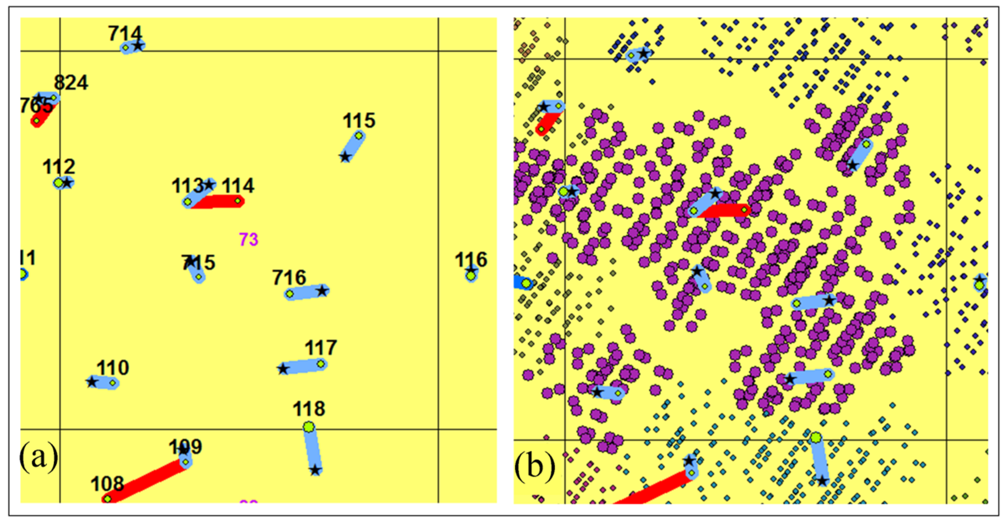
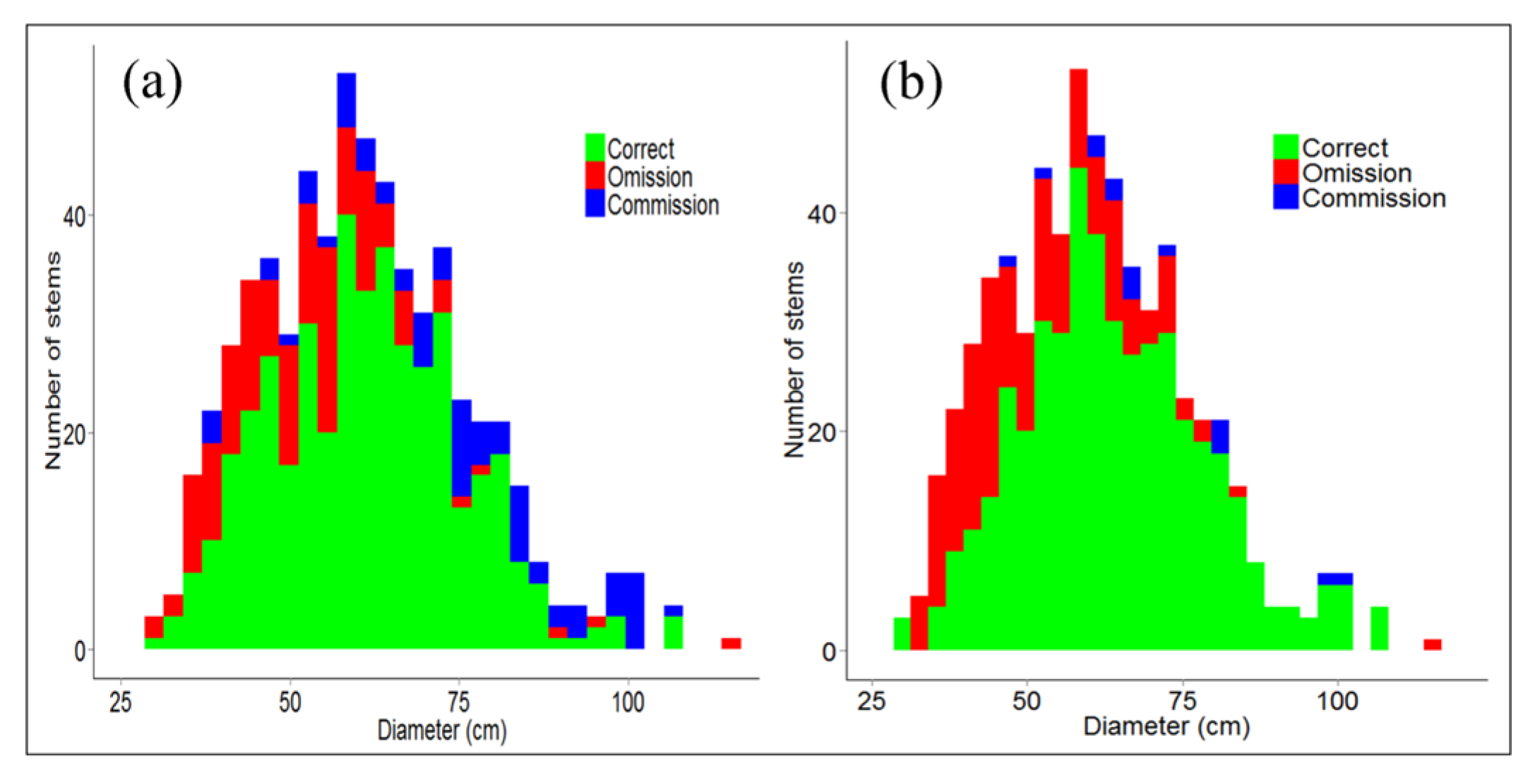
In this study, we have calibrated the NCut algorithm with one set of parameter values across a 5 ha 69 year old E. regnans forest. In order to apply the NCut algorithm across a broad range of existing age classes, age-specific calibration of the NCut algorithm will be required due to changes in forest structure with age. Even within one age class, substantial variation in canopy crown size was evident due to the spatial distribution of S_Den and BA_1.3, resulting in higher omission and commission rates within respectively high and low stocking density stands. Improved ITD rates may be achieved with a procedure that spatially varies the NCut parameter values with prior knowledge of the distribution of tree-crown forms across the landscape.

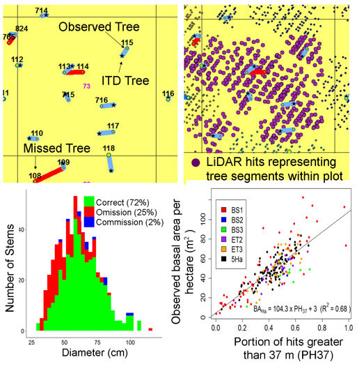
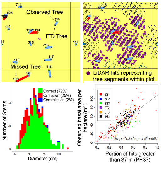
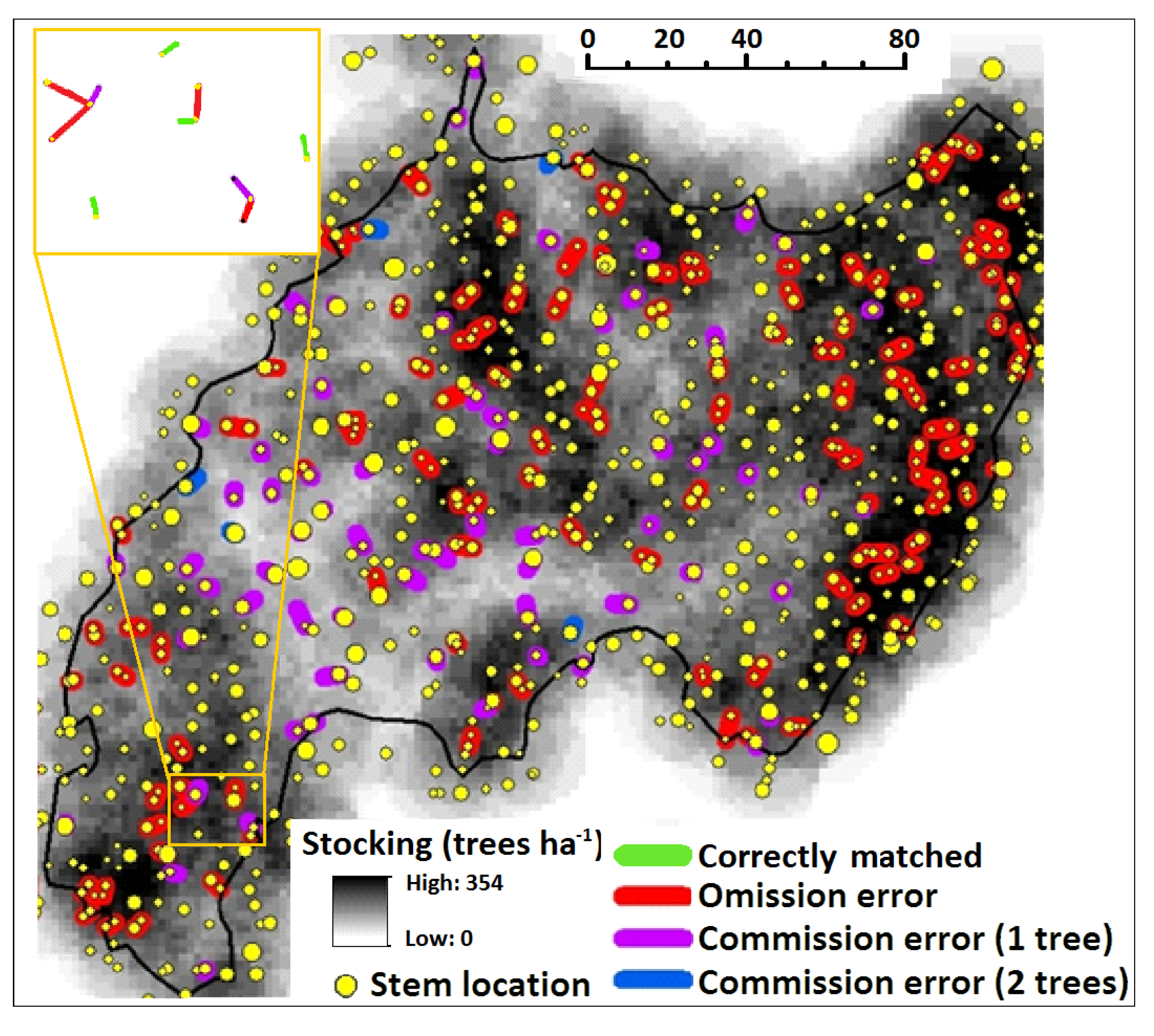
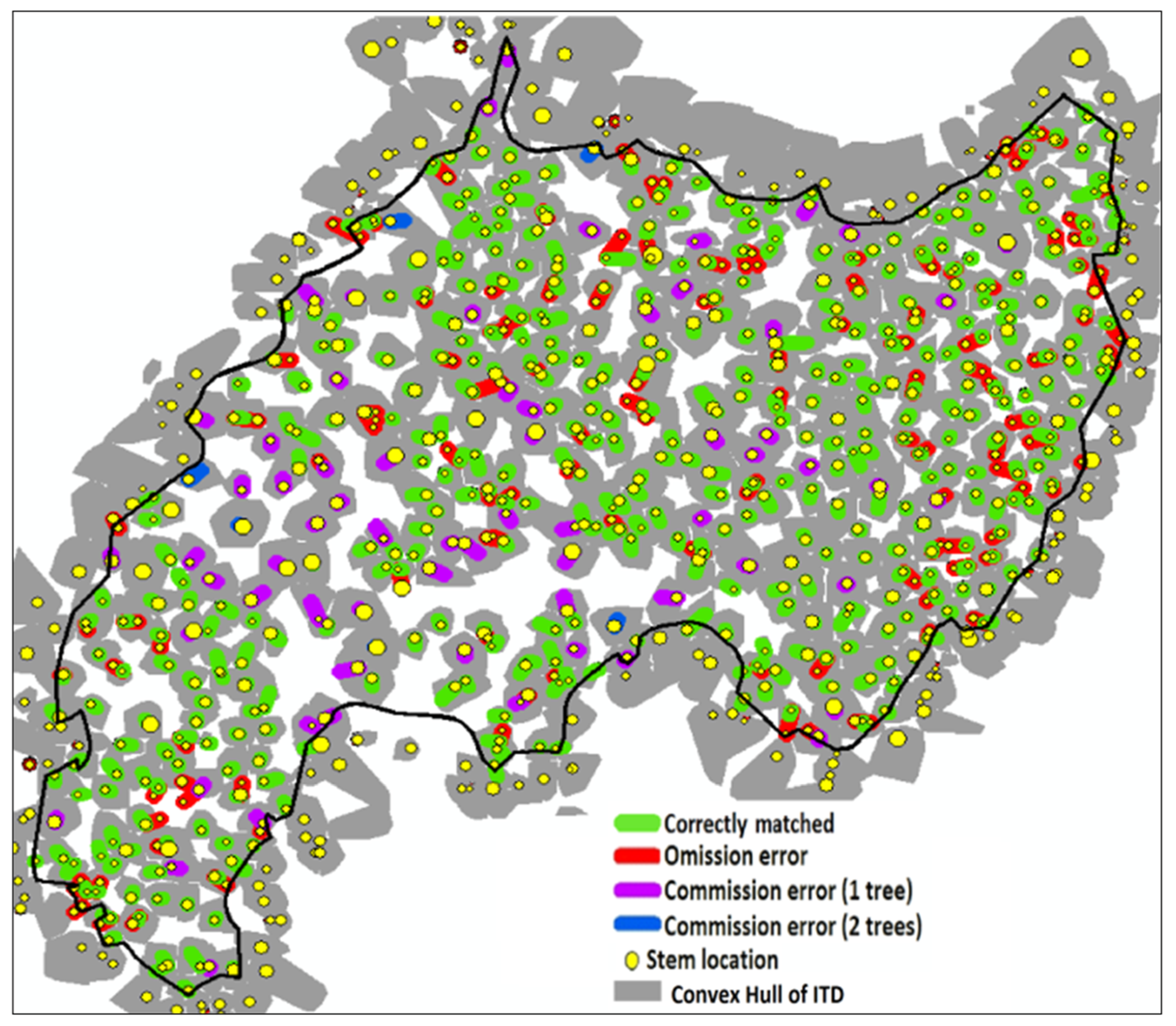
Figure 7 shows that this may be achieved with an efficient preliminary screening procedure capable of capturing the heterogeneity of canopy gaps across the landscape. Using each stem’s LiDAR points greater than 37 m, a 2D convex hull is provided in Figure 7 to show how well the heterogeneity in tree-crown form explains the distribution of stem commission and omission errors. Commission errors were more frequent in stands with large canopy gaps, as over-segmentation occurred for large tree canopies that extended towards large adjacent gaps.

To correct for this systematic S_Den bias, it would be necessary to segment the forested landscape into homogenous units characterised with canopy gap features and then apply varying sets of NCut parameter values calibrated to best segment forests with specific canopy gap features (see [48]). St-Onge et al. [49] have reviewed LiDAR based techniques that may be applied to automatically detect and characterise canopy gaps. The accuracy and resolution output of existing techniques is adequate for our purposes, considering [50] used an automated object-based technique to delineate canopy gaps with an accuracy of 96%, whereas [51] used multi-temporal LiDAR to identify newly opened gaps less than 1 m² in size.

Figure 7. A convex hull of each LiDAR segment, used to represent the crown canopy of each stem, showing that stems with commission error were adjacent to larger canopy gaps than stems with omission error.

Figure 7. A convex hull of each LiDAR segment, used to represent the crown canopy of each stem, showing that stems with commission error were adjacent to larger canopy gaps than stems with omission error.

4.2. Extrapolating SA_Ha over Large Water Supply Catchments

Stand BA represents a forest attribute commonly predicted with LiDAR data [52] and is regularly used in allometric relationships to predict SA [53]. We demonstrate that the NCut algorithm used in area-based estimates of BA_Ha is more accurate than the area-based mixture distribution function method, as we explained approximately 9% (median across five catchments) more BA_Ha variation. The improved performance was attributed to the NCut algorithm’s ability to generate plot-level indices with PLS segments that removed within-plot LiDAR points associated with trees found in adjacent plots and included LiDAR points in adjacent plots if they represented trees within the plots.

As well as predicting BA_Ha across a broad range of forest conditions (R² = 0.74; RMSE= 10.94), we provide a parsimonious model that is computationally efficient at accurately predicting BA_Ha with one explanatory variable, PH₃₇ (R² = 0.68; RMSE = 14.67). For extrapolating BA_Ha across large forested landscapes, the latter model is more appealing due to the intensive computational requirements of the NCut algorithm in the former model. For one hectare resolution BA_Ha estimates, we applied a pragmatic approach that involved calculating PH₃₇ from LiDAR points within 20 × 20 m grid cells, and then averaging the estimates using superimposed 100 m × 100 m grid cells. Averaging PH₃₇ reduced the propagated error generated when using a simplified calculation of PH₃₇ without the NCut algorithm to partition LiDAR points into PLS segments. Using this procedure to calculate PH₃₇, we applied the parsimonious model in Figure 5c to estimate BA_Ha across Melbourne’s Maroondah water supply catchments in Figure 8a.

Figure 8. Maps and histograms showing distribution of estimated (a) BA_Ha; (b) S_Den; and (c) SA_Ha of 1939 regrowth Ash forest across Melbourne’s Maroondah water supply catchment.

Figure 8. Maps and histograms showing distribution of estimated (a) BA_Ha; (b) S_Den; and (c) SA_Ha of 1939 regrowth Ash forest across Melbourne’s Maroondah water supply catchment.

Although it was more accurate to predict SA_Ha directly from LiDAR indices, the computational requirements of the NCut procedure (Table 5) may not justify the improved estimates (Figure 6). Using grids greater than 0.15 ha, [25] has shown that the perimeter index, $\sqrt{B{A}_{Ha}{S}_{Den}},$ accurately predicts SA_Ha (R² = 0.77, n = 15). In Table 6, we have shown that the computationally more efficient LMF method is capable of accurately predicting S_Den over a 5 ha site, which may further be improved using the relationship in (Figure 3 to correct for the systematic underestimation. Figure 8b provides the resulting S_Den map using this procedure. In (Figure 8c, SA_Ha across Melbourne’s Maroondah water supply catchment was calculated as [25]:

$$S{A}_{Ha}=0.0778\sqrt{B{A}_{Ha}{S}_{Den} }+1.05\left(R^2=0.77,n=15\right)$$

(7)

5. Conclusions

For even-aged forests, LiDAR data with as few as 0.9 pulses·m⁻² was able to be used with the LMF and NCut methods to determine S_Den and BA_Ha with moderate to high accuracy over large areas. Among 619 trees in a 69 year old E. regnans forest, the respective ITD rates were 72% and 68% using the LMF and NCut methods, with 25% and 20% of stems missed, and 2% and 12% of stems over-segmented. Given these similar ITD rates, we conclude that significantly lower computational requirements make the bias-corrected LMF method more suitable for predicting S_Den across large forest areas.

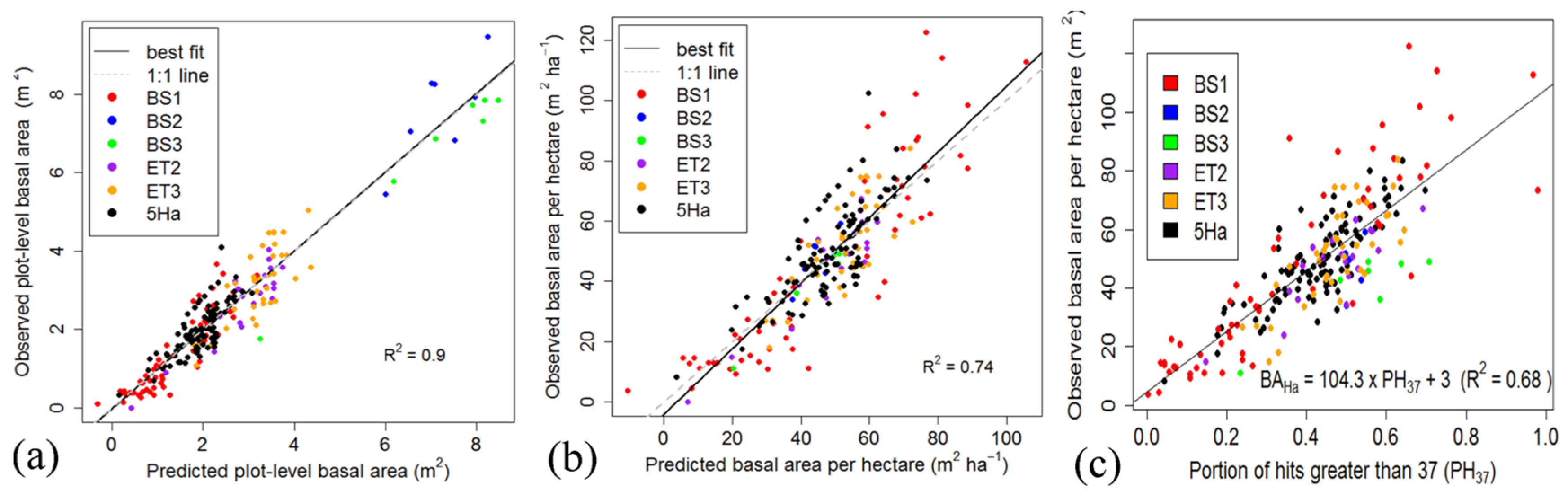
For estimating BA_Ha with plot resolution of the order of 0.04 ha, the NCut algorithm was a significant improvement over an area based method with mixture distribution functions, explaining 7% to 30% (median: 9%) more variation in BA_Ha for individual catchments. When applied to all catchments, we were able to produce a model that explained 68% of BA_Ha using only the PH₃₇ index that applies the NCut ITD segments. We demonstrate that this model may be extrapolated for one ha resolution estimates without the need to compute ITD segments. The two-step procedure involves calculating BA_Ha estimates by averaging PH₃₇ values calculated for each 20 m × 20 m grid cell over 100 m × 100 m grid cells.

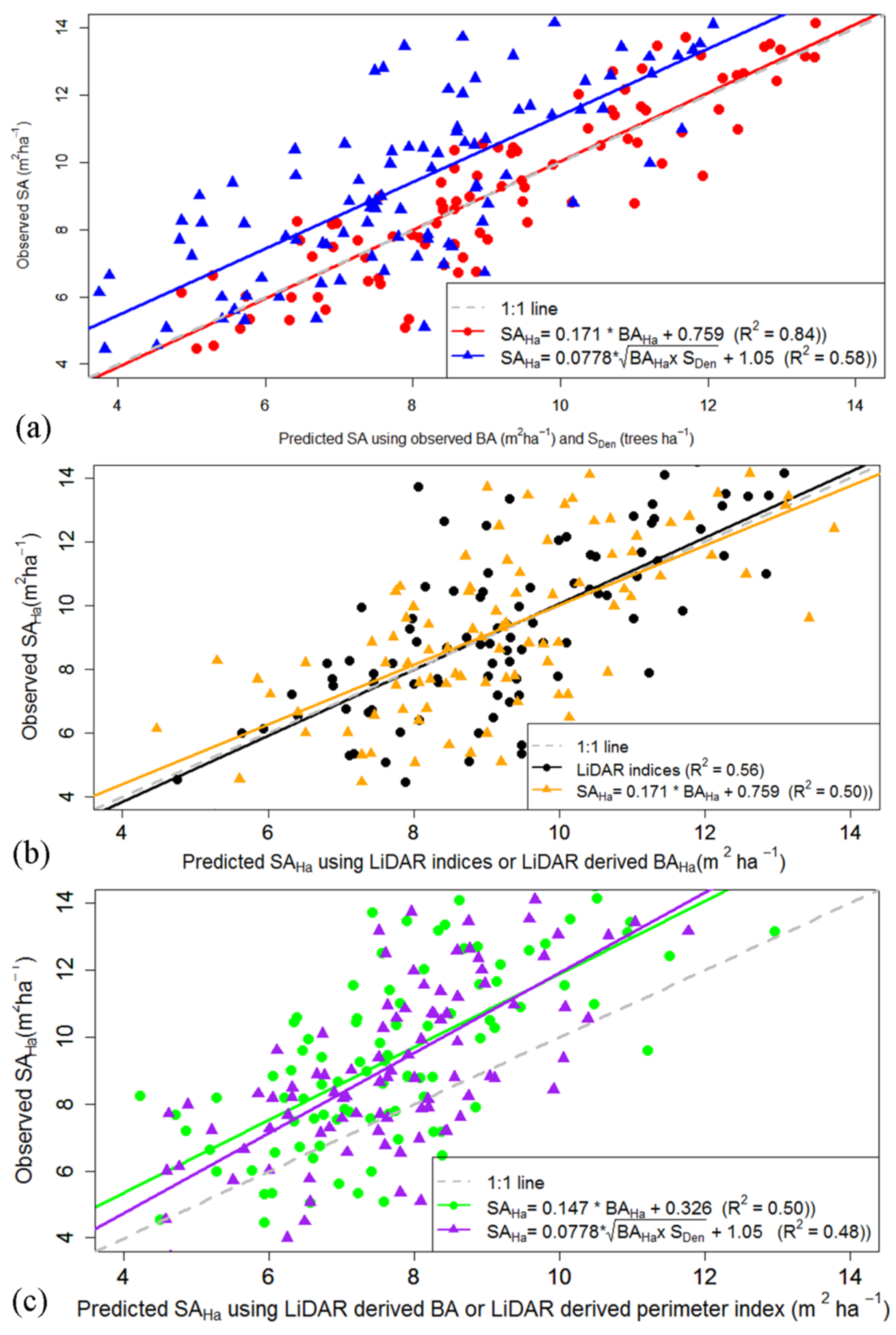
Although the relationship between observed and predicted SA_Ha was most accurate when directly relating SA_Ha to LiDAR indices (R² = 0.56), a two-step procedure that used the stem perimeter index to predict SA_Ha (R² = 0.48) was computationally more efficient. We conclude that a pragmatic approach for extrapolating SA_Ha across large water catchments involves using a one ha resolution grid to estimate: (i) S_Den with the bias-corrected LMF method; (ii) BA_Ha with a parsimonious model consisting of one explanatory variable, PH₃₇; and (iii) SA_Ha with the perimeter index using the BA_Ha and S_Den estimates.

References

1. Hyyppä, J.; Hyyppä, H.; Leckie, D.; Gougeon, F.; Yu, X.; Maltamo, M. Review of methods of small-footprint airborne laser scanning for extracting forest inventory data in boreal forests. Int. J. Remote Sens. 2008, 29, 1339–1366. [Google Scholar] [CrossRef]
2. Kuczera, G. Prediction of water yield reductions following a bushfire in ash-mixed species eucalypt forest. J. Hydrol. 1987, 94, 215–236. [Google Scholar] [CrossRef]
3. Cornish, P.M. The effects of logging and forest regeneration on water yields in a moist eucalypt forest in new south wales, Auastralia. J. Hydrol. 1993, 150, 301–322. [Google Scholar] [CrossRef]
4. Vertessy, R.A.; Watson, F.G.R.; O’Sullivan, S.K. Factors determining relations between stand age and catchment water balance in mountain ash forests. For. Ecol. Manag. 2001, 143, 13–26. [Google Scholar] [CrossRef]
5. Macfarlane, C.; Bond, C.; White, D.A.; Grigg, A.H.; Ogden, G.N.; Silberstein, R. Transpiration and hydraulic traits of old and regrowth eucalypt forest in southwestern Australia. For. Ecol. Manag. 2010, 260, 96–105. [Google Scholar] [CrossRef]
6. Haywood, A.; Stone, C. Using airborne laser scanning data to estimate structural attributes of natural eucalypt regrowth forests. Austral. For. 2011, 74, 4–12. [Google Scholar] [CrossRef]
7. Jaskierniak, D.; Lane, P.; Robinson, A.; Lucieer, A. Extracting lidar indices to characterise multilayered forest structure using mixture distribution functions. Remote Sens. Environ. 2011, 115, 573–585. [Google Scholar] [CrossRef]
8. Mitchell, P.J.; Lane, P.N.J.; Benyon, R.G. Capturing within catchment variation in evapotranspiration from montane forests using lidar canopy profiles with measured and modelled fluxes of water. Ecohydrology 2012, 5, 708–720. [Google Scholar] [CrossRef]
9. Kaartinen, H.; Hyyppä, J.; Yu, X.; Vastaranta, M.; Hyyppä, H.; Kukko, A.; Holopainen, M.; Heipke, C.; Hirschmugl, M.; Morsdorf, F.; et al. An international comparison of individual tree detection and extraction using airborne laser scanning. Remote Sens. 2012, 4, 950–974. [Google Scholar] [CrossRef] [Green Version]
10. Vauhkonen, J.; Ene, L.; Gupta, S.; Heinzel, J.; Holmgren, J.; Pitkänen, J.; Solberg, S.; Wang, Y.; Weinacker, H.; Hauglin, K.M.; et al. Comparative testing of single-tree detection algorithms under different types of forest. Forestry 2012, 85, 27–40. [Google Scholar] [CrossRef]
11. Kaartinen, H.; Hyyppa, J. EuroSDR/ISPRS Project, Commission II “Tree Extraction”; EuroSDR (European Spatial Data Research): Dublin, Ireland/Frankfurt, Germany, 2008; pp. 1–60. [Google Scholar]
12. Persson, A.; Holmgren, J.; Soderman, U. Detection and measuring individual trees using an airborne laser scanner. Photogram. Eng. Remote. Sens. 2002, 68, 925–934. [Google Scholar]
13. Maltamo, M.; Eerikäinen, K.; Pitkänen, J.; Hyyppä, J.; Vehmas, M. Estimation of timber volume and stem density based on scanning laser altimetry and expected tree size distribution functions. Remote Sens. Environ. 2004, 90, 319–330. [Google Scholar] [CrossRef]
14. Brandtberg, T.; Warner, T.; Landenberger, R.; McGraw, J. Detection and analysis of individual leaf-off tree crowns in small footprint, high sampling density lidar data from the eastern deciduous forest in north america. Remote Sens. Environ. 2003, 85, 290–303. [Google Scholar] [CrossRef]
15. Koch, B.; Heyder, U.; Weinacker, H. Detection of individual tree crowns in airborne lidar data. Photogramm. Eng. Remote Sens. 2006, 72, 357–363. [Google Scholar] [CrossRef]
16. Falkowski, M.J.; Smith, A.M.S.; Gessler, P.E.; Hudak, A.T.; Vierling, L.A.; Evans, J.S. The influence of conifer forest canopy cover on the accuracy of two individual tree measurement algorithms using lidar data. Can. J. Remote Sens. 2008, 34, S338–S350. [Google Scholar] [CrossRef]
17. Reitberger, J.; Krzystek, P.; Heurich, M.; Koukal, T.; Schneider, W. International Workshop on 3D Remote Sensing in Forestry Proceedings, 2006; Koukal, T., Schneider, W., Eds.; Institute of Surveying, Remote Sensing and Land Information: Vienna, Austria; p. 218.
18. Morsdorf, F.; Meier, E.; Allgower, B.; Nuesch, D. Clustering in airborne laster scanning raw data for segmentation of single trees. Int. Arch. Photogramm. Remote Sens. Spat. Inf. Sci. 2003, 24, 27–33. [Google Scholar]
19. Persson, Å.; Holmgren, J.; Söderman, U.; Olsson, H. Tree species classification of individual trees in sweden by combining high resolution laser data with high resolution near infrared digital images. Int. Arch. Photogramm. Remote Sens. Spat. Inf. Sci. 2004, XXXVI, 204–207. [Google Scholar]
20. Solberg, S.; NÆsset, E.; Bollandsas, O.M. Single tree segmentation using airborne laser scanner data in a structurally heterogeneous spruce forest. Photogramm. Eng. Remote Sens. 2006, 72, 1369–1378. [Google Scholar] [CrossRef]
21. Pyysalo, U.; Hyyppä, H. Reconstructing tree crowns from laser scanner data for feature extraction. Int. Arch. Photogramm. Remote Sens. Spat. Inf. Sci. 2002, 34, 218–221. [Google Scholar]
22. Wang, Y.; Weinacker, H.; Koch, B.; Sterenczak, K. Lidar point cloud based fully automatic 3D single tree modelling in forest and evaluations of the procedure. Int. Arch. Photogramm. Remote Sens. Spat. Inf. Sci. 2008, 37, 45–51. [Google Scholar]
23. Reitberger, J.; Schnörr, C.; Krzystek, P.; Stilla, U. 3D segmentation of single trees exploiting full waveform lidar data. ISPRS J. Photogramm. Remote Sens. 2009, 64, 561–574. [Google Scholar] [CrossRef]
24. Yao, W.; Krzystek, P.; Heurich, M. Enhanced Detection of 3D Individual Trees in Forested Areas Using Airborne Full-Waveform Lidar Data by Combining Normalised Cuts with Spatial Density Clustering. In Proceedings of the ISPRS Annals of the Photogrammetry, Remote Sensing and Spatial Information Sciences, Antalya, Turkey, 11–13 November 2013.
25. Jaskierniak, D.; Kuczera, G.; Benyon, R.J.; Lucieer, A. Spatial variation of tree and stand sapwood area in southeastern australian forests. J. Plant Ecol. 2014. Submitted. [Google Scholar]
26. Jaskierniak, D.; Benyon, R.; Kuczera, G.; Robinson, A. A new method for measuring stand sapwood area in forests. Ecohydrology 2014. [Google Scholar] [CrossRef]
27. Axelsson, P. Processing of laser scanner data—Algorithms and applications. ISPRS J. Photogramm. Remote Sens. 1999, 54, 138–147. [Google Scholar] [CrossRef]
28. Kraus, K.; Pfeifer, N. Determination of terrain models in wooded areas with airborne scanner data. ISPRS J. Photogramm. Remote Sens. 1999, 54, 193–203. [Google Scholar]
29. Hutchinson, M.F. A new procedure for gridding elevation and stream line data with automatic removal of spurious pits. J. Hydrol. 1989, 106, 211–232. [Google Scholar] [CrossRef]
30. Shi, J.; Malik, J. Normalized cuts and image segmentation. IEEE Trans. Pattern Anal. Mach. Intell. 2000, 22, 888–905. [Google Scholar]
31. Wikipedia. Eucalyptus Regnans. Available online: http://en.wikipedia.org/wiki/Eucalyptus_regnans (accessed on 01 June 2015).
32. R Core Team. R: A Language and Environment for Statistical Computing; R Foundation for Statistical Computing: Vienna, Austria, 2013. [Google Scholar]
33. Akaike, H. New look at statistical-model identification. IEEE Trans. Automat. Control 1974, 716, 716–723. [Google Scholar] [CrossRef]
34. Ben-Arie, J.R.; Hay, G.J.; Powers, R.P.; Castilla, G.; st-Onge, B. Development of a pit filling algorithm for lidar canopy height models. Comput. Geosci. 2009, 35, 1940–1949. [Google Scholar] [CrossRef]
35. Hyyppa, J.; Kelle, O.; Lehikoinen, M.; Inkinen, M. A segmentation-based method to retrieve stem volume estimates from 3-d tree height models produced by laser scanners. IEEE Trans. Geosci. Remote Sens. 2001, 39, 969–975. [Google Scholar] [CrossRef]
36. Yao, W.; Krzystek, P.; Heurich, M. A Sensitivity Analysis for a Novel Individual Tree Segmentation Algorithm Using 3d Lidar Point Cloud Data; Silvilaser: Vancouver, BC, Canada, 2012; pp. 1–13. [Google Scholar]
37. Lundgren, J. Alpha Shapes. In MATLAB Central File Exchange. 2010. Available online: http://www.Mathworks.Com.Au/matlabcentral/fileexchange/28851-alpha-shapes/content/alphavol.M (accessed on 01 April 2015).
38. Hastie, T.; Tibshirani, R.; Friedman, J. The Elements of Statistical Learning: Data Mining, Inference, and Prediction; Springer-Verlag: New York, NY, USA, 2001. [Google Scholar]
39. Golub, G.; Heath, M.; Wahba, G. Generalised cross-validation as a method for choosing a good ridge parameter. Technometrics 1979, 21, 215–223. [Google Scholar] [CrossRef]
40. Efron, B.; Tibshirani, R. Improvements on cross-validation. The 0.632+ bootstrap method. J. Am. Stat. Assoc. 1997, 2, 548–560. [Google Scholar]
41. Florence, R.G. Ecology and Silviculture of Eucalypt Forests; CSIRO Publishing: Melbourne, Australia, 1996; p. 413. [Google Scholar]
42. Ford, C.R.; Hubbard, R.M.; Kloeppel, B.D.; Vose, J.M. A comparison of sap flux-based evapotranspiration estimates with catchment-scale water balance. Agric. For. Meteorol. 2007, 145, 176–185. [Google Scholar] [CrossRef]
43. Loranty, M.M.; Mackay, D.S.; Ewers, B.E.; Adelman, J.D.; Kruger, E.L. Environmental drivers of spatial variation in whole-tree transpiration in an aspen-dominated upland-to-wetland forest gradient. Water Resourc. Res. 2008, 44, W02441. [Google Scholar] [CrossRef]
44. Dunn, G.M.; Connor, D.J. An analysis of sap flow in mountain ash (eucalyptus regnans) forests of different age. Tree Physiol. 1993, 13, 321–336. [Google Scholar] [CrossRef] [PubMed]
45. Haydon, S.R.; Benyon, R.G.; Lewis, R. Variation in sapwood area and throughfall with forest age in mountain ash (eucalyptus regnans f. Muell.). J. Hydrol. 1996, 187, 351–366. [Google Scholar] [CrossRef]
46. Lahivaara, T.; Seppanen, A.; Kaipio, J.P.; Vauhkonen, J.; Korhonen, L.; Tokola, T.; Maltamo, M. Bayesian approach to tree detection based on airborne laser scanning data. IEEE Trans. Geosci. Remote Sens. 2014, 52, 2690–2699. [Google Scholar] [CrossRef]
47. Yu, X.; Litkey, P.; Hyyppä, J.; Holopainen, M.; Vastaranta, M. Assessment of low density full-waveform airborne laser scanning for individual tree detection and tree species classification. Forests 2014, 5, 1011–1031. [Google Scholar] [CrossRef]
48. Palenichka, R.M.; Zaremba, M.B. Multiscale isotropic matched filtering for individual tree detection in lidar images. IEEE Trans. Geosci. Remote Sens. 2007, 45, 3944–3956. [Google Scholar] [CrossRef]
49. St-Onge, B.; Vepakomma, U.; Sénécal, J.-F.; Kneeshaw, D.; Doyon, F. Canopy gap detection and analysis with airborne laser scanning. In Forestry Applications of Airborne Laser Scanning; Maltamo, M., Næsset, E., Vauhkonen, J., Eds.; Springer: Dordrecht, The Netherlands, 2014; Volume 27, pp. 419–437. [Google Scholar]
50. Vepakomma, U.; st-Onge, B.; Kneeshaw, D. Spatially explicit characterization of boreal forest gap dynamics using multi-temporal lidar data. Remote Sens. Environ. 2008, 112, 2326–2340. [Google Scholar] [CrossRef]
51. St-Onge, B.; Vepakomma, U. Assessing forest gap dynamics and growth using multi-temporal laser-scanner data. In Proceedings of the Laser-Scanners for Forest and Landscape Assessment—Instruments, Processing Methods and Applications International Conference, Freiburg, Germany, 3–6 October 2004; pp. 173–178.
52. Lefsky, M.A.; Cohen, W.B.; Acker, S.A.; Parker, G.G.; Spies, T.A.; Harding, D. Lidar remote sensing of the canopy structure and biophysical properties of douglas-fir western hemlock forests. Remote Sens. Environ. 1999, 70, 339–361. [Google Scholar] [CrossRef]
53. Vertessy, R.A.; Benyon, R.G.; O’Sullivan, K.; Gribben, P.R. Relationships between stem diameter, sapwood area, leaf area and transpiration in a young mountain ash forest. Tree Physiol. 1995, 15, 559–567. [Google Scholar] [CrossRef] [PubMed]