Article

Mapping Flooded Rice Paddies Using Time Series of MODIS Imagery in the Krishna River Basin, India

by
Pardhasaradhi Teluguntla
1,*,
Dongryeol Ryu
1,*,
Biju George
1,2,
Jeffrey P. Walker
3 and
Hector M. Malano
1
1
Department of Infrastructure Engineering, The University of Melbourne, Victoria 3010, Australia
2
Integrated Water & Land Management Program, ICARDA, Cairo P.O. Box 2416, Egypt
3
Department of Civil Engineering, Monash University, Victoria 3800, Australia
*
Authors to whom correspondence should be addressed.
Remote Sens. 2015, 7(7), 8858-8882; https://doi.org/10.3390/rs70708858
Submission received: 23 March 2015 / Revised: 16 June 2015 / Accepted: 30 June 2015 / Published: 13 July 2015

Abstract

:
Rice is one of the major crops cultivated predominantly in flooded paddies, thus a large amount of water is consumed during its growing season. Accurate paddy rice maps are therefore important inputs for improved estimates of actual evapotranspiration in the agricultural landscape. The main objective of this study was to obtain flooded paddy rice maps using multi-temporal images of Moderate Resolution Imaging Spectroradiometer (MODIS) in the Krishna River Basin, India. First, ground-based spectral samples collected by a field spectroradiometer, CROPSCAN, were used to demonstrate unique contrasts between the Normalized Difference Vegetation Index (NDVI) and the Land Surface Water Index (LSWI) observed during the transplanting season of rice. The contrast between Enhanced Vegetation Index (EVI) and Land Surface Water Index (LSWI) from MODIS time series data was then used to generate classification decision rules to map flooded rice paddies, for the transplanting seasons of Kharif and Rabi rice crops in the Krishna River Basin. Consistent with ground spectral observations, the relationship of the MODIS EVI vs. LSWI of paddy rice fields showed distinct features from other crops during the transplanting seasons. The MODIS-derived maps were validated against extensive reference data collected from multiple land use field surveys. The accuracy of the paddy rice maps, when determined using field plot data, was approximately 78%. The MODIS-derived rice crop areas were also compared with the areas reported by Department of Agriculture (DOA), Government of India (Government Statistics). The estimated root mean square difference (RMSD) of rice area estimated using MODIS and those reported by the Department of Agriculture over 10 districts varied between 3.4% and 6.6% during 10 years of our study period. Some of the major factors responsible for this difference include high noise of the MODIS images during the prolonged monsoon seasons (typically June–October) and the coarse spatial resolution (500 m) of the MODIS images compared to the small crop fields in the basin. However, this study demonstrates, based on multi-year analysis, that MODIS images can still provide robust and consistent flooded paddy rice extent and areas over a highly heterogeneous large river basin.

Graphical Abstract

1. Introduction

Evapotranspiration (ET) from irrigated crop areas comprises the biggest anthropogenic consumption of fresh water in the world. Irrigation is known to consume about 70–80 percent of all water used by humans [1]. It is therefore important to estimate current irrigation water use accurately, not only for water resources assessment but also for the prediction of future water demand. Among all the irrigated crops, flooded paddy rice has drawn particular interest due to the large population living on rice consumption and its unique cultivation method, especially in Asia. Rice feeds more than half of the entire population of the world [1,2] and the cultivation of paddy rice on flooded soils requires large quantities of fresh water, which has significant implications to water security and terrestrial water balance. Moreover, waterlogged soils are one of the largest sources of methane gas emissions [3,4,5]. Mapping rice paddies is thus a critical component for developing environmentally sustainable water management [6,7].
Currently available land-cover and land-use maps based on satellite sensors, such as global land cover maps based on Landsat and Moderate Resolution Imaging Spectroradiometer (MODIS) produced by the Global Land Cover Facility (GLCF, http://www.landcover.org), do not provide detailed sub-classes within the class of agricultural fields. However, the unique flooded farming method of rice can be utilized to discriminate the paddy rice fields from other agricultural fields. Particularly, during the transplanting season of rice, a significant fraction of the rice paddies consists of ponded surface water, resulting in strong water reflectance. Even though detecting ponded surfaces using only visible (red) and near infrared (NIR) bands that are commonly used to classify vegetation types is not straightforward, it can be aided by using the Land Surface Water Index (LSWI) [8]. The LSWI is calculated using spectral signals in shortwave infrared (SWIR) and near infrared (NIR) ranges to detect water at the soil surface [9] and the vegetation water content [10,11].
Previous works [8,12,13,14] have compared NDVI or the Enhanced Vegetation Index (EVI) with LSWI during the transplant season to map paddy rice fields in China, South Asia and Southeast Asia. Xiao et al. [8] analyzed the multi-temporal SPOT-4 satellite imagery (Vegetation 10-day composite images, 1-km resolution) collected over Jiangsu, China to map flooded paddy rice fields, where pixels with LSWI greater than NDVI were classified as paddy rice. Xiao et al. [12,13] used multi-temporal MODIS images (8-day composites, MOD09A1, 500-m resolution) to extend the approach to larger regions in South China, South Asia and Southeast Asia. They used a relaxed set of criteria, LSWI + 0.05 > EVI or LSWI + 0.05 > NDVI, to identify flooded paddy rice fields. The mapped paddy rice fields were overall in good agreement with census statistics and regional land cover maps derived from the Landsat ETM+, although some discrepancies in land classes existed. The errors were attributed to cloud contamination of optical images, topographic effects, and low spatio-temporal resolution of the images. Sun et al. [14] provided more detailed multi-year LSWI vs. EVI relationships in paddy rice fields depending on the planting season of the crop. Recently, Gumma et al. [15] mapped rice area in South Asia using spectral matching techniques, which were fully based on MODIS NDVI time-series data.
Previous studies reported that the coarse spatial and temporal resolution of satellite observations used is an important source of error in identifying flooded rice fields. The ground coverage of rice increases steeply within a few weeks from transplanting and NDVI quickly saturates to its near-maximum values [16]. Moreover, due to the typically small size of paddies in South and Southeast Asian countries, most 500-m MODIS pixels contain mixed flooded rice, non-flooded crops and other vegetation. The MODIS SWIR bands required to calculate LSWI are available for 500-m spatial resolution. Consequently, the sub-pixel-scale heterogeneity can seriously degrade the performance of the NDVI (or EVI)/LSWI-based paddy-rice-mapping. In order to examine NDVI-vs.-LSWI behavior free from the effect of the sub-pixel-scale heterogeneity, it is therefore necessary to analyze field spectral samples collected from various crop covers and growth stages. Ground-based spectral samples can play a critical role [17,18] in developing and calibrating an algorithm to map rice paddies. Note that the previous works reviewed (e.g., [12,13,14]) developed algorithms directly on the assumed relationship between satellite-based NDVI (and EVI) and LSWI without presenting their actual relationship over homogeneous fields.
In this study, spectral samples of flooded paddy rice at various growth stages, along with those of non-paddy crops, were collected from the Musi sub-basin of the Krishna River Basin in India (Figure 1) using an MSR 16 CROPSCAN spectroradiometer to demonstrate behavioral features of NDVI and LSWI. After confirming a distinctive NDVI vs. LSWI relationship for paddy rice and non-paddy crops, flooded rice paddies are mapped using the time series of three indices—NDVI, LSWI and EVI—derived from the 8-day composite of MODIS data (MOD09A1). Consequently, decision rules for Kharif rice and Rabi rice were developed from a subset of the observed data using LSWI and EVI, the rules were then applied on MODIS data over the whole study area, and the spatial distribution of paddy rice maps for the Kharif and Rabi seasons finally produced over the Basin.
Figure 1. Ground survey locations of paddy rice fields used for rice algorithm where land use survey and the CROPSCAN-based spectral sampling were conducted in the Krishna River Basin.
Remotesensing 07 08858 g001

2. Study Area and Dataset
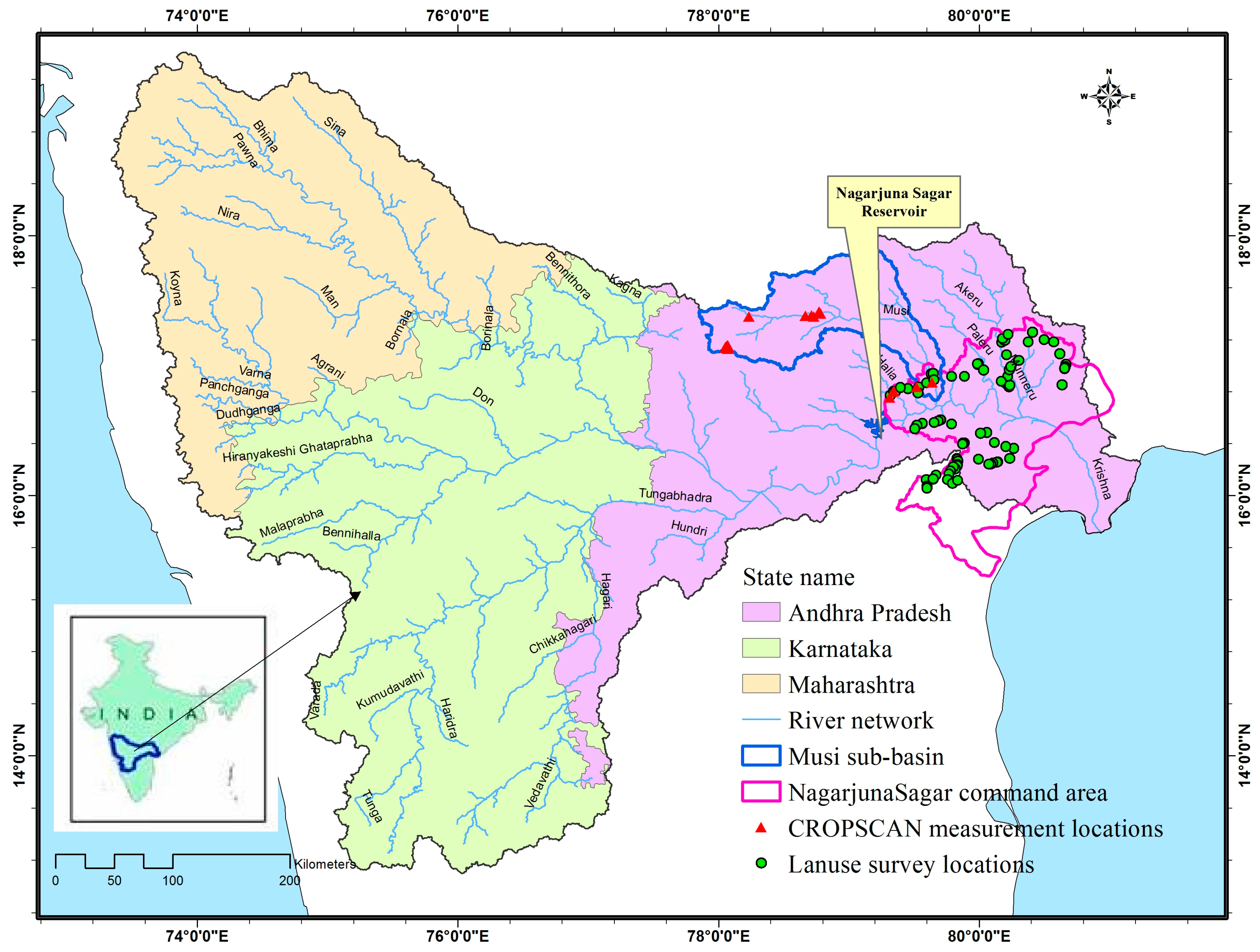
2.1. Study Area

The Krishna River Basin (Figure 1) is the fourth largest river basin in India in terms of drainage area, located in the southern part of India between longitudes 73°15′E and 81°15′E, and latitudes 13°05′N and 19°20′N. The total geographical area is 265,752 km2, covering the three states of Karnataka, Maharashtra and Andhra Pradesh. The River Krishna originates in the Western Ghats Mountains, flows east across the Deccan Plateau, and discharges into the Bay of Bengal. It has three main tributaries that drain from the northwest, west, and southwest (Figure 1). The climate is dominantly semi-arid, with some dry, sub-humid areas in the eastern delta and humid areas in the Western Ghats. Annual precipitation is 800 mm on average. Most of the rainfall occurs during the Indian monsoon from June to October [19,20]. Crops are grown in three seasons, during the monsoon (June to mid-December), called Kharif, in the post-monsoon dry season (mid-December to March) called Rabi, and dry summer period (April and May) [19,20]. Compared to Kharif and Rabi, the short dry summer period, called Zaid, comprises a very small fraction of the total rice production thus will not be considered for the land cover classification of this work. Major irrigated crops include single/double cropping rice, single cropping sugarcane, chili, cotton, pulses, fodder grass, and some light irrigated corn, sorghum and sunflower. Rainfed crops include grains (sorghum, millet), pulses (red and green gram, chickpea), and oilseeds (sunflower, groundnut). In the large irrigation command areas, such as Almatti, Tungabhadra, Ujjani-Bhima, Jurala, Nagarjuna Sagar, and Prakasam (Krishna Delta), crop fields are irrigated during the Kharif and Rabi seasons. Major canal irrigation schemes occur along each of the major reservoirs in the upper basin, and along the main drainage in the lower basin and in the delta (Figure 1), which are predominant rice growing areas. Minor irrigated systems include small tanks, small riparian lift schemes, and ground water irrigation. Ground water sources include dug wells, shallow tube wells, and deep tube wells. We conducted intensive land use surveys at different crop growth stages in the Nagajuna Sagar irrigation command (Figure 1), which is located in the eastern part of the basin. Ground-based spectral samples were collected from the Musi sub-basin located in the northeastern part of the basin.

2.2. Datasets and Description

2.2.1. Field Spectral Samples

In order to demonstrate and confirm the unique NDVI vs. LSWI relationship of flooded paddy rice, which were utilized to map rice paddies in previous works, a spectral library of paddy rice at different growth stages were taken from ground-based spectral samples using a portable multispectral radiometer (model MSR16) manufactured by CROPSCAN, Inc. The MSR16 used in this work collects 12 bands, six bands from sky and six bands from ground targets, providing on-site calibrated surface reflectance at six wavelengths ranging from 530 nm to 1640 nm. It is assumed that the irradiance flux density incident on the sky-facing radiometers is identical to the flux density incident to the target surface. Specifications of the spectral data are summarized in Table 1.
Table 1. Wavelength of spectral bands equipped in the CROPSCAN 16 (MSR16R) and their equivalent bands of Moderate Resolution Imaging Spectroradiometer (MODIS).
MSR16R BandsSub-DivisionCentre Wavelength (nm)Band Width (nm)MODIS Bands
Band 1Visible5308.5Band 11
Band 2Visible5709.7
Band 3Visible65040.0Band 1
Band 4NIR85540.0Band 2
Band 5MIR124011.6Band 5
Band 6SWIR164015.5Band 6
An intensive ground sampling was conducted as a part of the Australia-India Land Surface Parameterisation Experiment for Remote Sensing (AILSPEX-RS) during February 2011 (AILSPEX-11) and September 2012 (AILSPEX-12) in the Musi sub-basin of the Krishna River Basin in India [17]. The first experiment period captured the transplanting season of Rabi (winter, dry cropping season) in the region and the second experiment captured the peak growing season of Kharif. A comprehensive database was constructed for the field spectral sample survey. Information collected for each site includes:
  • Location information (GPS position, location name, date of collection).
  • Land use (crop type).
  • Vegetation height.
  • 12-band reflectance measurements by CROPSCAN.
  • Land surface temperature measured by the thermal infrared scanner.
  • Soil temperature at the depths of 1 cm, 5 cm and 10 cm.
  • Soil moisture content in the top 5 cm by the theta probe soil moisture sensor (model ML2 by Delta-T Devices Ltd.).
  • Digital photographs.
The data collected from this experiment was used to identify unique features of rice paddies and to justify the rice paddy identification criteria from MODIS imagery. LSWI and NDVI were produced over the paddy rice fields and surrounding non-flooded crop fields, and analyzed with varying crop height.

2.2.2. MODIS Surface Reflectance Data

The MODIS 8-day composite product from Terra (MOD09A1) was used in this work. From the seven bands of MOD09A1 product at 500 m resolution (Table 2), four bands (blue, red, NIR and SWIR) captured the seasonal variations in vegetation vigor, soil and vegetation moisture and surface water that characterize the key stages of rice cultivation [13,21].
Table 2. Specifics of the MODIS-Terra bands (MOD09A1) used in this study 1.
MODIS Bands 2Band Width (nm)Centre Wavelength (nm)Sub DivisionPotential Application 3
3459–479470BlueSoil/Vegetation Differences
1620–670648RedAbsolute Land Cover Transformation, Vegetation Chlorophyll
2841–876858NIRCloud Amount, Vegetation Land Cover Transformation
61628–16521640SWIRSnow/Cloud Differences
Note: 1 Out of the 36 MODIS bands, the first seven bands are specially processed for Land studies; 2 MODIS bands are re-arranged to follow the electromagnetic spectrum (e.g., blue band 3 followed by red band 1); 3 Source: http://modis-land.gsfc.nasa.gov.
The reflectance data have undergone several pre-processing steps, including algorithms for atmospheric correction. The 8-day composite MODIS product with 500-m spatial resolution (MOD09A1) was downloaded from http://modis-land.gsfc.nasa.gov for the period of June 2000 to May 2010. A total of 46 composites were available each year. For each 8-day composite, the following indices were calculated using surface reflectance values from the blue, red, near infrared (NIR) and shortwave infrared (SWIR) bands (see Table 2) NDVI, EVI [21], and LSWI [12,13].
N D V I = N I R R E D N I R + R E D
E V I = 2.5 N I R R E D N I R + 6 × R E D 7.5 × B L U E + 1
L S W I = N I R S W I R N I R + S W I R

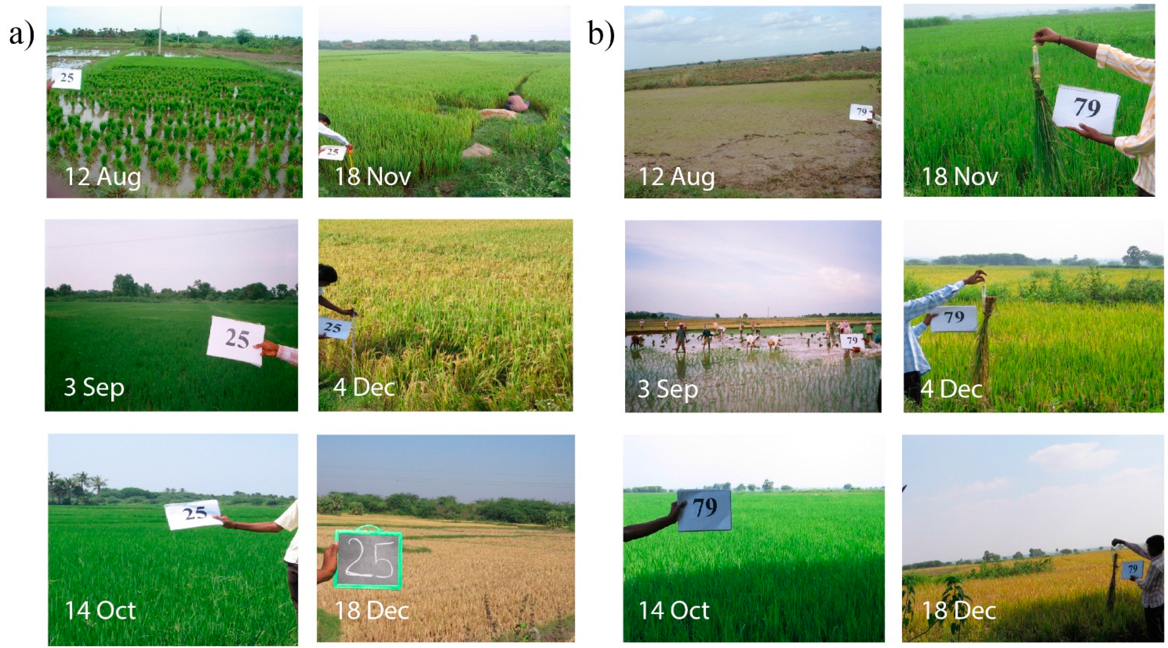
2.2.3. Field Survey of Land Use

In order to obtain characteristic EVI vs. LSWI for flooded paddy rice and non-paddy crops, and also to validate the paddy rice map of this study, we have used information collected from 91 sampling sites in the northeastern part of the Krishna River Basin were used (see Figure 1, Land use survey locations) during Kharif and Rabi in 2006–2007. Ground-based satellite validation can be complicated by the sub-pixel-scale surface heterogeneity. In order to reduce the impact of the heterogeneity, field survey sites were chosen over relatively homogeneous cropping fields. The sampling sites include various crop fields: irrigated rice, cotton, chili, sugarcane, turmeric, grams, etc. All of the sites are located within a major surface water irrigated area called the Nagarjuna Sagar irrigation command. A total of eight field surveys were conducted at different crop growth stages. A comprehensive database constructed from the field survey includes:
  • Location information (GPS position, location name, date of collection).
  • Land use/land cover type (class name).
  • Fraction of individual land cover types such as cropped canopy and no canopy area (water, fallow lands and weeds) within each crop field.
  • Crop types, cropping pattern and cropping calendar (i.e., Kharif, Rabi and summer seasons).
  • Agricultural intensification, sources of water and presence of irrigated, rain-fed and supplemental irrigation.
  • Characteristics of crops such as plant height, soil texture, and density of plants per square meter;
  • Digital photographs.
Some of the photos showing growth stages of two paddy rice fields (Sites 25 and 79) in the Nagarjuna Sagar irrigation command area are shown in Figure 2. The first photo in Figure 2a,b shows the rice paddies during the transplanting season, where a large fraction of ponded field was exposed when compared to other growth stages. The fraction of ponded surface is gradually decreasing with the increase in vegetation cover.

2.2.4. Agricultural Statistical Data

District level agricultural census data for the current study area (in 2000–2010) were obtained from the Directorate of Economics and Statistics (DES), Department of Agriculture (DOA), Government of India (http://apy.dacnet.nic.in). The database contains district level statistics on cropping area, production and productivity of each crop. The district-wise statistics of paddy rice area in each year, along with the field survey data, were used to validate the paddy rice maps produced from the satellite imagery in this work.
Figure 2. (a) Photos of the paddy rice site #25 (transplantation date of 12 August) at different growth stages in 2006–2007 Kharif season. (b) Photos of the paddy rice site #79 (transplantation date of 3 September) at different growth stages in 2006–2007 Kharif season.
Remotesensing 07 08858 g002

3. Methods

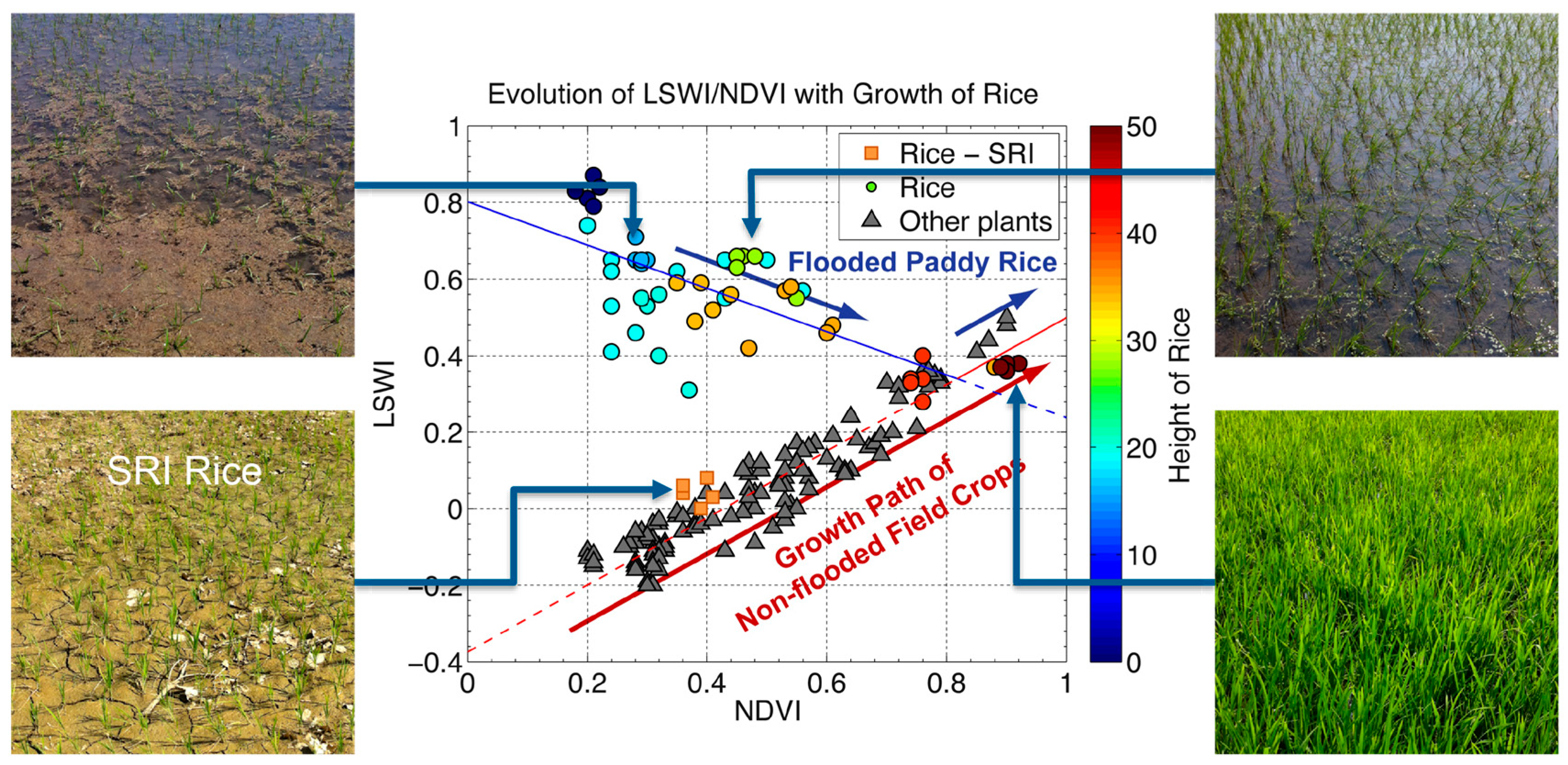
3.1. Growth Stages of Rice

The cropping period of rice varies between 4 and 6 months in the Krishna River Basin, depending on the rice variety. In general, paddy fields are ploughed and flooded before rice transplanting. Rice grows rapidly after transplantation with the temporal dynamics of paddy rice fields characterized by three main periods: flooding/transplanting period, cropping period (vegetative growth, reproductive and ripening stages) and the fallow period after harvest. During the rice transplant period, the land surface is a mixture of surface water and green plants with water depth ranging from 5 to 20 cm. About 50 to 60 days after transplanting, the rice canopy grows and covers most of the cultivated surface area. From the start of end of the growth period, leaf and stem moisture content start decreasing. The NDVI and EVI of paddy fields decrease during the transplanting period and then increase for the rest of the growing season, whereas LSWI steeply increases during the transplanting season. According to time-series data of the spectral reflectance of paddy fields [22], the NDVI and EVI reaches a maximum around the heading date as the rice crop changes its growth phase from vegetative growth to reproductive growth on reaching the heading date, and the leaves begin to wither. NDVI and EVI then decrease abruptly because of harvesting.

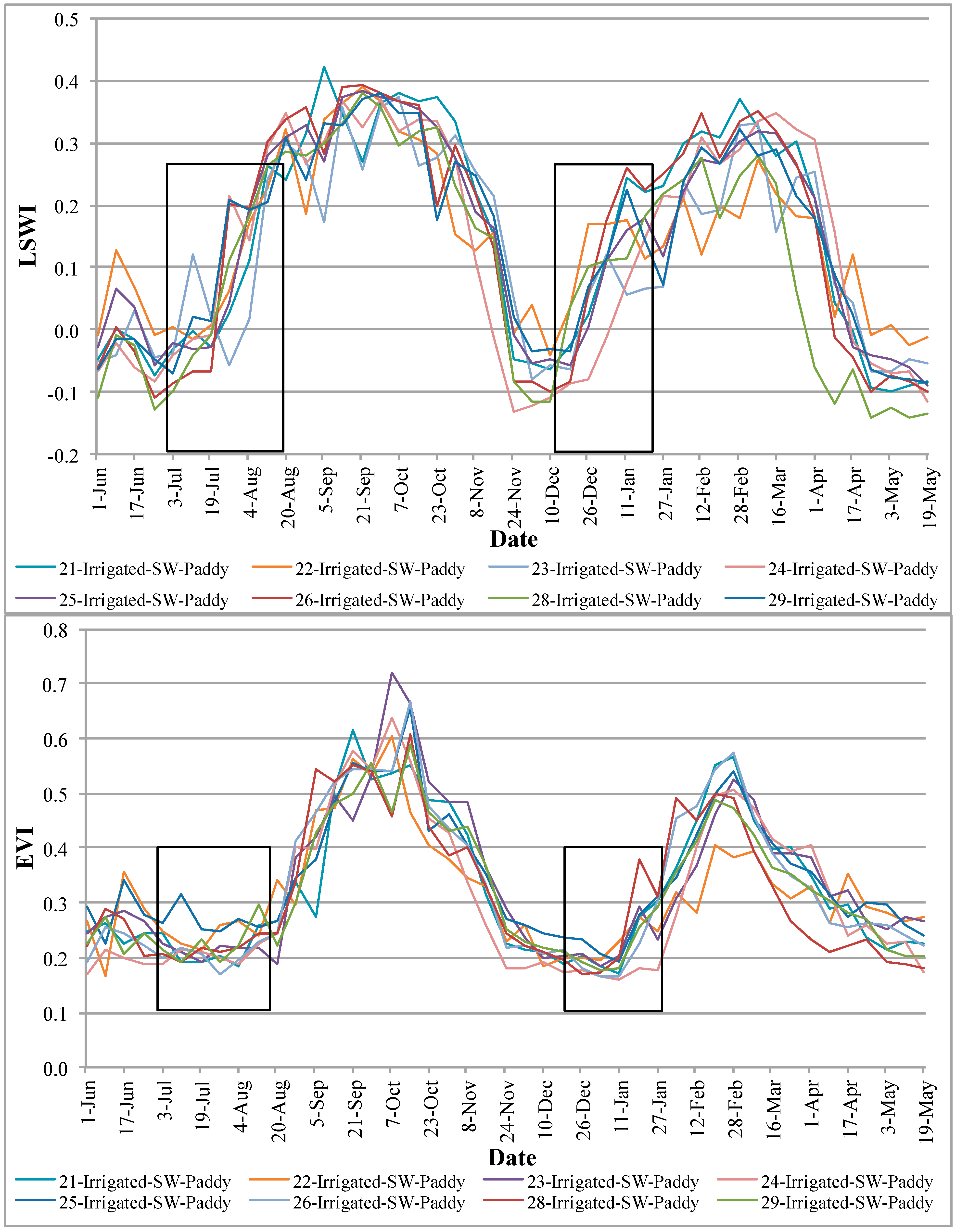
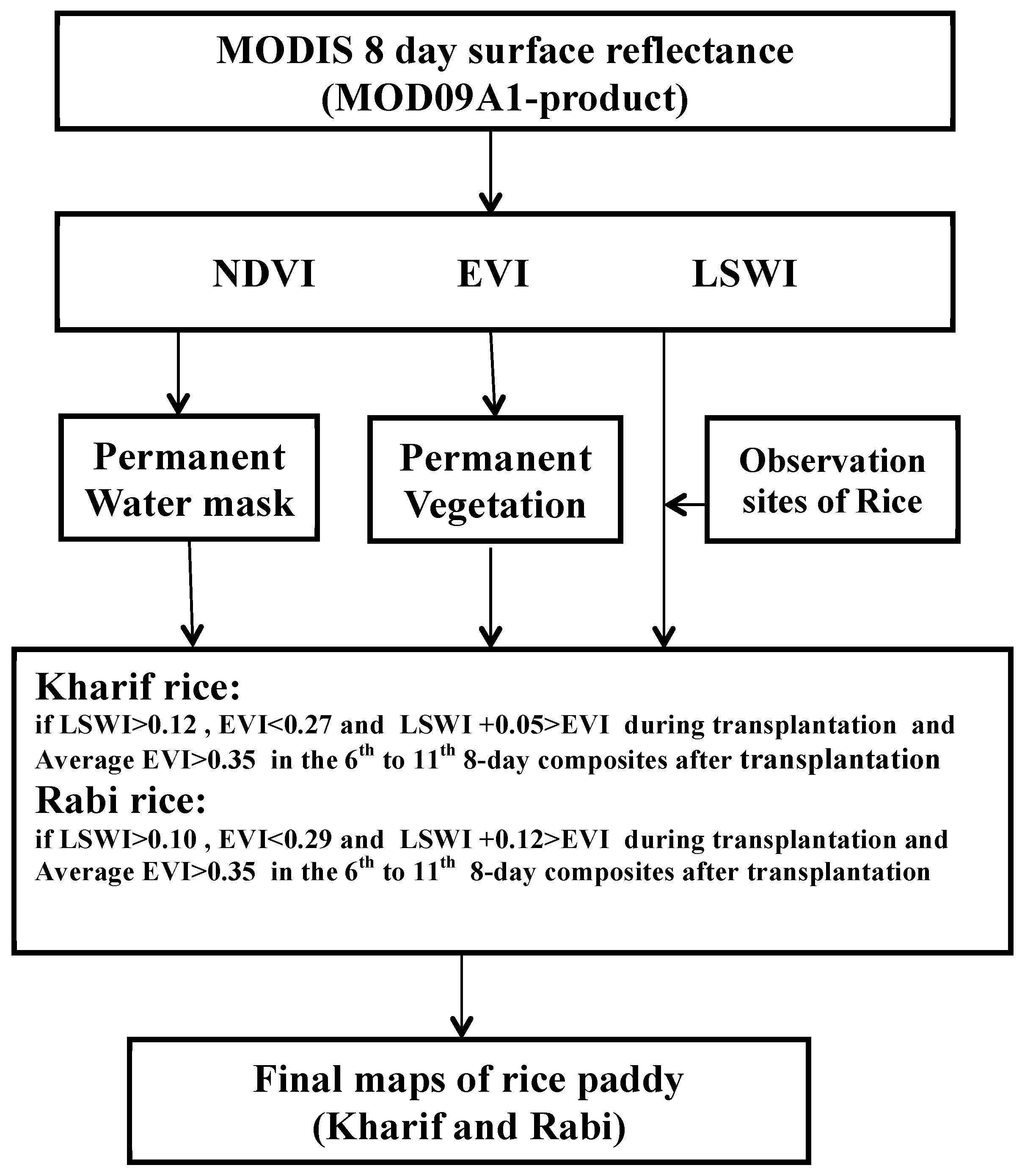
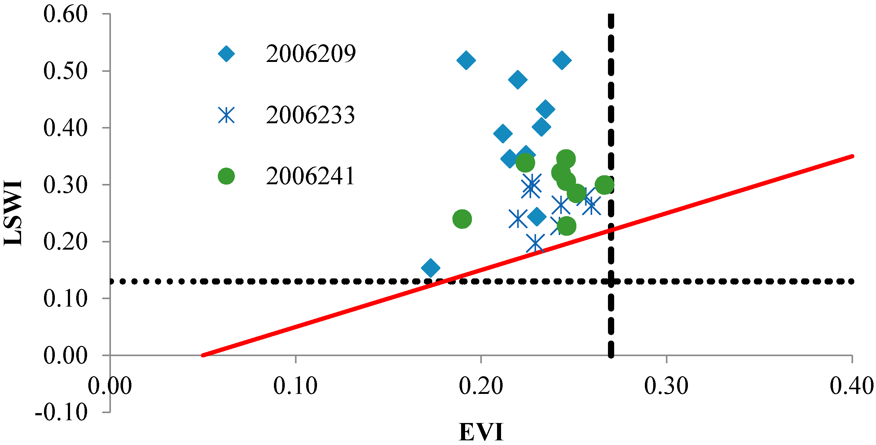
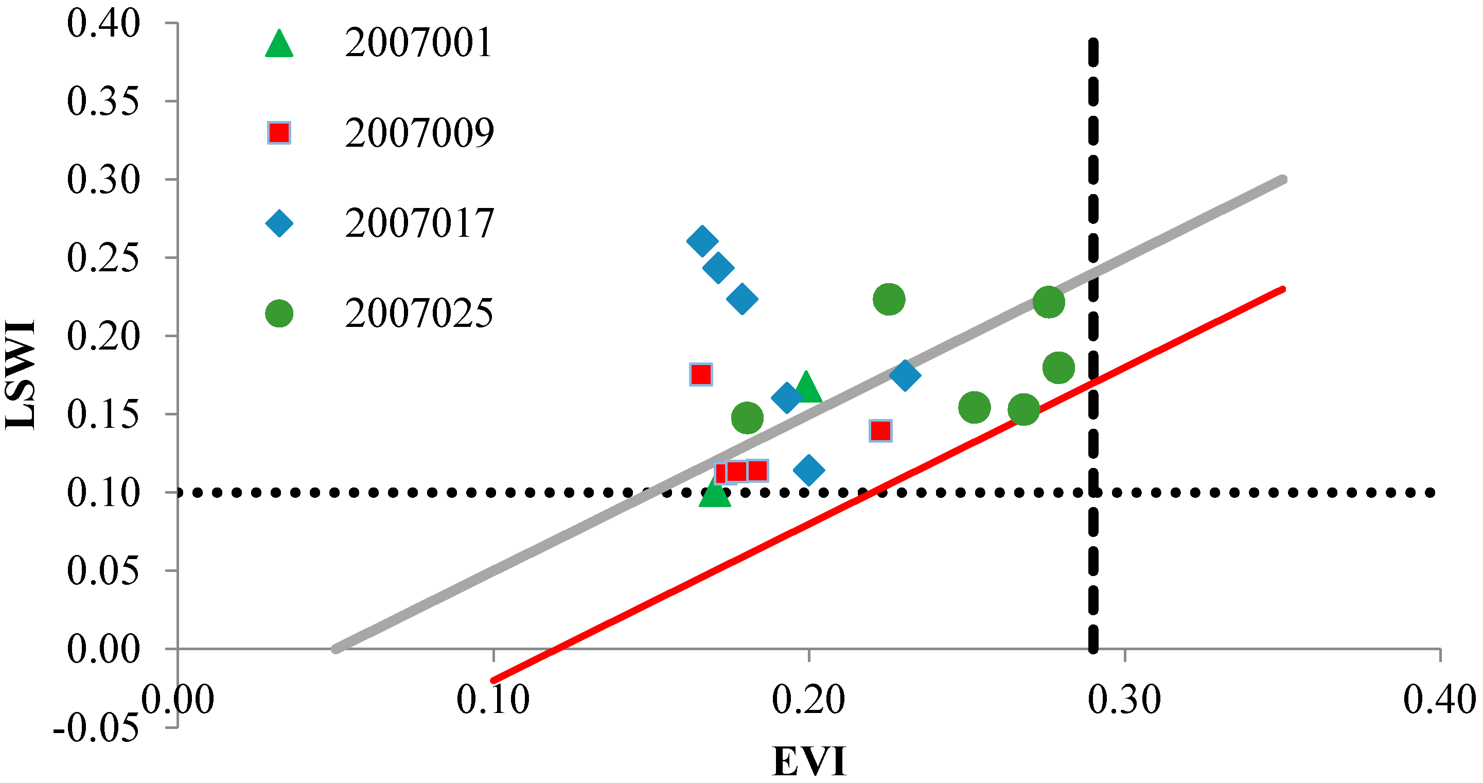
3.2. Identification of Flooded Paddy Rice

Rice fields are filled with water at the beginning of the transplanting season and remain ponded until approximately 1–2 weeks before harvest. However, due to the large fraction of water surface during the transplanting season, reflectance in the short-wavelength infrared (SWIR) range, which is sensitive to water, can be used to distinguish the flooded rice paddies from other crops. Thus, in order to detect the transplanting date, which follows flooding in paddy rice fields, using the time profile of EVI or NDVI and LSWI, existence of the period when a temporary inversion of NDVI/EVI and where LSWI becomes higher than EVI or NDVI values or approaches closer, can be used.
Due to the locally and regionally varying irrigation schedules in the basin, the transplanting occurs over a period of nearly 60 days from July through September for Kharif and from December through February for Rabi rice. Consequently, at least six to eight MODIS 8-day composite images are needed for each season to discriminate rice paddies, which are based on our field surveys, ground based spectral data collected from field experiments (see Section 4.1 for more details) and agriculture statistical information collected from different parts of the river basin.
Identification of changes in the mixture of surface water and vegetation canopies in paddy rice fields over time requires spectral bands or vegetation indices that are sensitive to both water and vegetation. NDVI is closely correlated with the Leaf Area Index (LAI) of paddy rice fields [11] but is sensitive to aerosols. However, EVI directly adjusts the reflectance in the red band as a function of the reflectance in the blue band, accounting for residual atmospheric contamination and variable soil and canopy background reflectance [21]. Consequently, EVI is known to be much less sensitive to aerosols than NDVI and so in this work, EVI is chosen instead of NDVI for the vegetation change detection. The SWIR band is sensitive to leaf water content and soil moisture and is used to develop improved water sensitive indices such as LSWI, which combines NIR with SWIR bands and has the capability of retrieving canopy water content [23,24]. The strong light absorption by liquid water in the SWIR (Band 6 of MODIS) range makes LSWI sensitive to the total amount of liquid water in vegetation and its soil background [9]. The Band 5 of MODIS (1230–1250 nm) is also sensitive to soil water content, but it is not used to detect LSWI because of weaker sensitivity than Band 6. Although the 8-day composite surface reflectance products of MODIS have been pre-processed to reduce the impacts of clouds, shadows, and aerosols, there remain residual noises due to atmospheric effect and heavy clouds in some regions. Algorithms used for removing noise in time-series methods include moving median or average and Fourier-based algorithms [25,26]. In this work, contaminated pixels were identified by abrupt changes in NDVI with time and were substituted by one of the values in the temporally adjacent images based on validity or by the average of the adjacent images when both of them are valid. If the pixels in both the adjacent images are contaminated, then those pixels are discarded.
Due to the prolonged heavy monsoon rains in the study area, temporary flooding can occur during the Kharif season. Xiao et al. [12,13] used the conditions LSWI + 0.05 ≥ EVI or LSWI + 0.05 ≥ NDVI for identifying rice paddy fields on the basis of transplanting period, irrespective of the acquired date of the images. An auxiliary condition was also used: the EVI value reaches half of the maximum EVI value within five 8-day composites following the flooding and transplanting period [12,13]. Moreover, the non-rice area was further removed using the digital elevation model (DEM) data and masks of cloud, permanent water, and permanent/evergreen vegetation. This method is expected to avoid the need of identifying various transplanting schedules over a region. However, it can overestimate the rice fields due to the other irrigated crops or temporary flooding due to rainfall. Moreover, Kharif rice and Rabi rice cannot be separated if they are planted in the same fields in a hydrological year.
To resolve these problems, MODIS data were integrated with prior information on the rice growth calendar obtained from field observations in different zones of the basin. The data were obtained from the Department of Agriculture (DOA), the Command Area Development Authority (CADA) and the Reservoir Monitoring Authorities. The planting calendar is relatively similar to the rice growth calendar with small inter-annual variations, thus all potential dates of the flooding and transplanting period in different zones are selected based on the calendars of 2000–2010. As the calendars of the plants in other croplands might be different from the rice calendar, so the noise in the images beyond the transplanting period (e.g., strong water signal) could be eliminated. After harvesting the Kharif rice, the rice fields are kept fallow for approximately 2–4 weeks before the Rabi season starts, or they are cultivated with short-term dry crops. Based on the cropping patterns of the study region, the available MODIS 8-day composite images in a hydrological year were partitioned into two seasons to generate Kharif and Rabi rice maps, consequently to produce separate categories for single crop (Kharif or Rabi) and double cropped rice (Kharif and Rabi) fields.
The reflectance over these areas is the mixture of paddy rice fields (composed of water, soil, seedlings, etc.) and the background (roads, weeds, other crops, etc.) in the rice-transplanting period. The characteristics of high water and low coverage of vegetation can be detected by comparing LSWI and EVI, since they feature relatively high LSWI and low EVI in this period. Areas of high EVI in this period are regarded as non-rice vegetation fields (trees, shrubs, grass, etc.). In order to obtain characteristic EVI vs. LSWI for flooded paddy rice and non-paddy crops, we examined time series of 8-day EVI and LSWI over the 20 rice and 20 non-rice sites in different regions of our study area including double crop rice (Figure 3) and single crop rice (Figure 4) grown areas. Average EVI and LSWI at each test site during the flooding and transplanting period (for Kharif and Rabi) were calculated. The decision rules for mapping rice are LSWI > 0.12, EVI < 0.27, and LSWI > (EVI − 0.05) for Kharif rice, and LSWI > 0.10, EVI < 0.29, and (LSWI + 0.12) > EVI for Rabi rice (with increased the relaxation from 0.05 to 0.12, see Section 4.2). An additional condition was applied to the initial rice-paddy pixels to remove permanent water bodies: the pixels with EVI ≤ 0.35 in the 6th~11th 8-day MODIS EVI composites following the transplanting period were flagged as permanent water bodies. These conditions were used to generate rice paddy maps for both Kharif and Rabi crops for the entire study region. An overview of the overall approach for mapping rice paddies for Kharif and Rabi seasons is shown in Figure 5 in the form of a flow diagram.
Figure 3. Time series of LSWI and EVI of observed rice fields in the double crop rice zones. The vertical lines represent transplantation season, during this period we can observe inversion of indices for flooded paddy rice pixels.
Remotesensing 07 08858 g003
Figure 4. Time series of LSWI and EVI of observed rice fields in the single crop rice zones. The vertical lines represent transplantation season, during this period we can observe inversion of indices for flooded paddy rice pixels.
Remotesensing 07 08858 g004
Figure 5. An overview of procedure used for identification of flooded paddy rice using MODIS data for Kharif and Rabi seasons shown in a systematic diagram.
Remotesensing 07 08858 g005

4. Results and Discussion

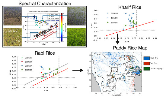
4.1. Spectral Characteristics from Ground Reflectance

The main aim of collecting ground reflectance data was to compare the distinct features of NDVI vs. LSWI between the paddy rice and other non-flooded crop fields. Even though a steep increase of LSWI paired with a decrease of NDVI during the transplant season was inferred from their general behavior and used to map rice paddies in previous works, it has not been shown explicitly using ground samples over the systematically varied homogeneous fields. The spectral responses from two categories of fields are summarized in Figure 6. The results show that LSWI of non-rice crops increases linearly with NDVI in general. The strong linear relationship between the indices is due to the dominant impact of vegetation water content and the non-flooded nature on the observed LSWI in the non-rice fields. In contrast with the other non-flooded crops, LSWI of the paddy rice fields showed decreasing trend with NDVI. Even though LSWI is scattered widely around the linear fit, LSWI decreased linearly with NDVI until the NDVI of rice reached approximately 0.75. The two linear models intersected at the point where the NDVI value is 0.85. It also appears that LSWI of paddy rice joins the increasing trend with NDVI beyond the threshold NDVI value. At full canopy cover the influence of ponded water on reflectivity becomes insignificant resulting in both LSWI and NDVI showing high values. The decreasing trend of LSWI is mainly due to that the fact that the spectral signal coming directly from the ponded surface in the back ground decreases with the growth of rice. During initial growth stages (canopy cover < 100%), the flooded paddy fields absorb both NIR and red heavily, resulting in low NDVI values whereas in LSWI the SWIR band absorption is relatively low (compared to NIR or red), resulting in high LSWI values. This contrast between LSWI and NDVI during initial growth stages in ponded paddy fields provides contrasting supplementary information, leading to an improved ability in separation of flooded rice from other crops. For paddy rice fields, the decreasing LSWI with increasing NDVI is highly correlated with the height of the rice (Figure 6).
Figure 6. Comparison of indices (NDVI and LSWI) for samples collected in the paddy rice and the other non-flooded crop fields (AILSPEX-11, AILSPEX-12).
Remotesensing 07 08858 g006
The results from the analysis in Figure 6 also shows that examining the trends between NDVI and LSWI are more informative for discriminating paddy rice fields than simply comparing the magnitude of the normalized indices, as was adopted by the previous works. The LSWI values are greater than NDVI only up until the height of the rice reaches approximately 20 cm (Figure 6). However, the spectral samples from the paddy rice exhibit clear distinction from the values of other fields up to NDVI = 0.6, which is equivalent to 35 cm of crop height. The observed difference in the crop height ranges can be used to discriminate paddy rice fields, but only when the rice crop is less than 35 cm tall. With the given limits on temporal scales of satellite images when using the 8-day composite imagery of MODIS for mapping, a larger time window for mapping is gained by explicit LSWI-NDVI analysis when it is assumed that the rice grows linearly with time just after transplanting. Figure 6 shows that plots of paddy rice can be better separated from the other fields while a number of LSWI and NDVI values are mixed when the height of rice is greater than 10 cm.

4.2. Decision Rules for Mapping Kharif and Rabi Rice Paddy Using MODIS Indices

The results from the analysis in Figure 7 and Figure 8 show the thresholds of MODIS EVI and MODIS LSWI for the paddy rice fields during transplantation period for Kharif and Rabi seasons. Based on these thresholds, we obtained the final set of decision rules for mapping Kharif and Rabi rice using MODIS 500 m datasets. The decision rules obtained for mapping rice are LSWI > 0.12, EVI < 0.27, and LSWI > (EVI − 0.05) (Figure 7) for Kharif rice, and LSWI > 0.10, EVI < 0.29, and (LSWI + 0.12) > EVI for Rabi rice (with increased the relaxation from 0.05 to 0.12, Figure 8). These conditions were then used to generate rice paddy maps for both Kharif and Rabi seasons using MODIS 500 m datasets. Also an additional condition was applied to the initial rice-paddy pixels to remove permanent water bodies: the pixels with EVI ≤ 0.35 in the 6th~11th 8-day MODIS EVI composites following the transplanting period, were flagged as permanent water bodies.
Figure 7. Characteristics of paddy rice fields reflected by EVI and LSWI in the transplanting period according to ground observation sites during 2006–2007 Kharif season. The red line is the threshold for potential rice in the transplantation season based on our analysis.
Remotesensing 07 08858 g007
Figure 8. Characteristics of paddy rice fields reflected by EVI and LSWI in the transplanting period according to ground observation sites during 2006–2007 Rabi season. The red line is the threshold for potential rice in the transplantation season of Rabi, whereas the green line was threshold used for Kharif.
Remotesensing 07 08858 g008

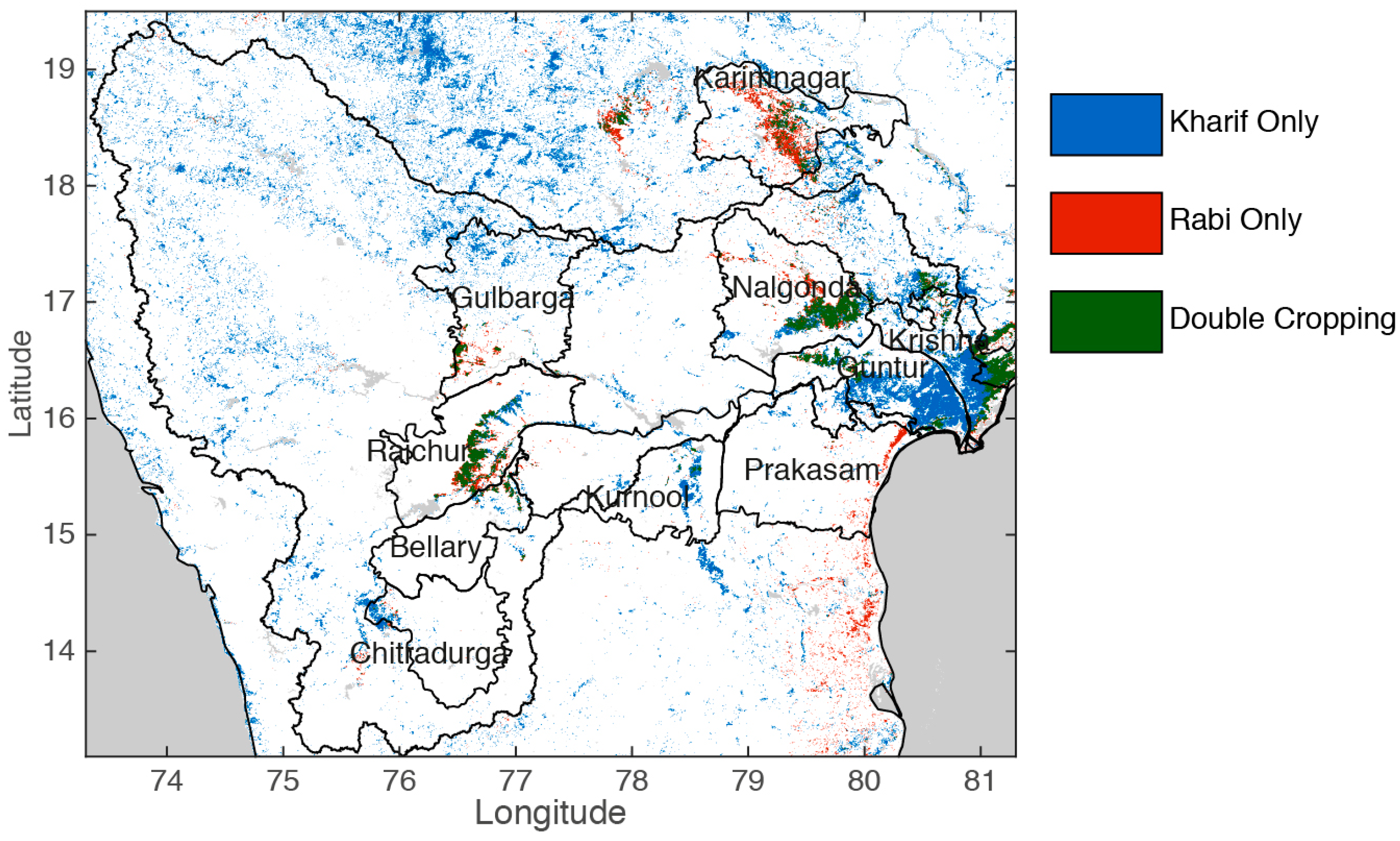
4.3. Spatial Distribution of MODIS-Derived Rice Paddies

The maps of Kharif and Rabi rice paddies were derived from MODIS data using the algorithm explained above. The classification results of 2006–2007 Kharif and Rabi rice fields were shown in Figure 9. The map shows four classes. Blue represents only Kharif-rice, red represents only Rabi-rice and green represents double crop rice (i.e., both Kharif and Rabi rice). The maps were validated using two types of data: field survey data and national statistics of rice cropping areas.
Figure 9. Spatial distribution of Kharif and Rabi paddy rice areas derived using MODIS 500-m datasets in the Krishna River Basin during 2006–2007. Boundaries of the districts chosen for statistical evaluation (used in Section 4.7) are overlaid.
Remotesensing 07 08858 g009

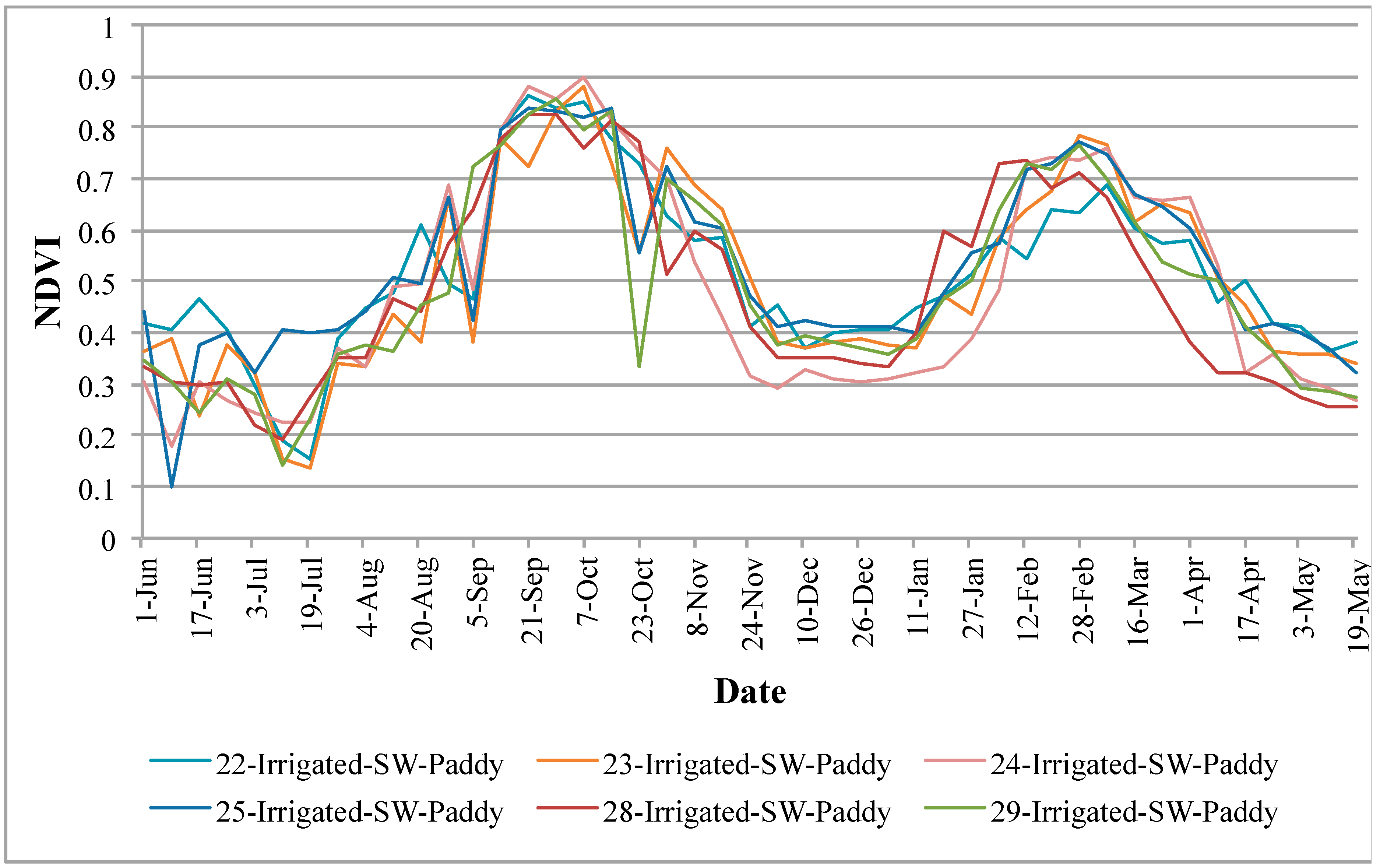
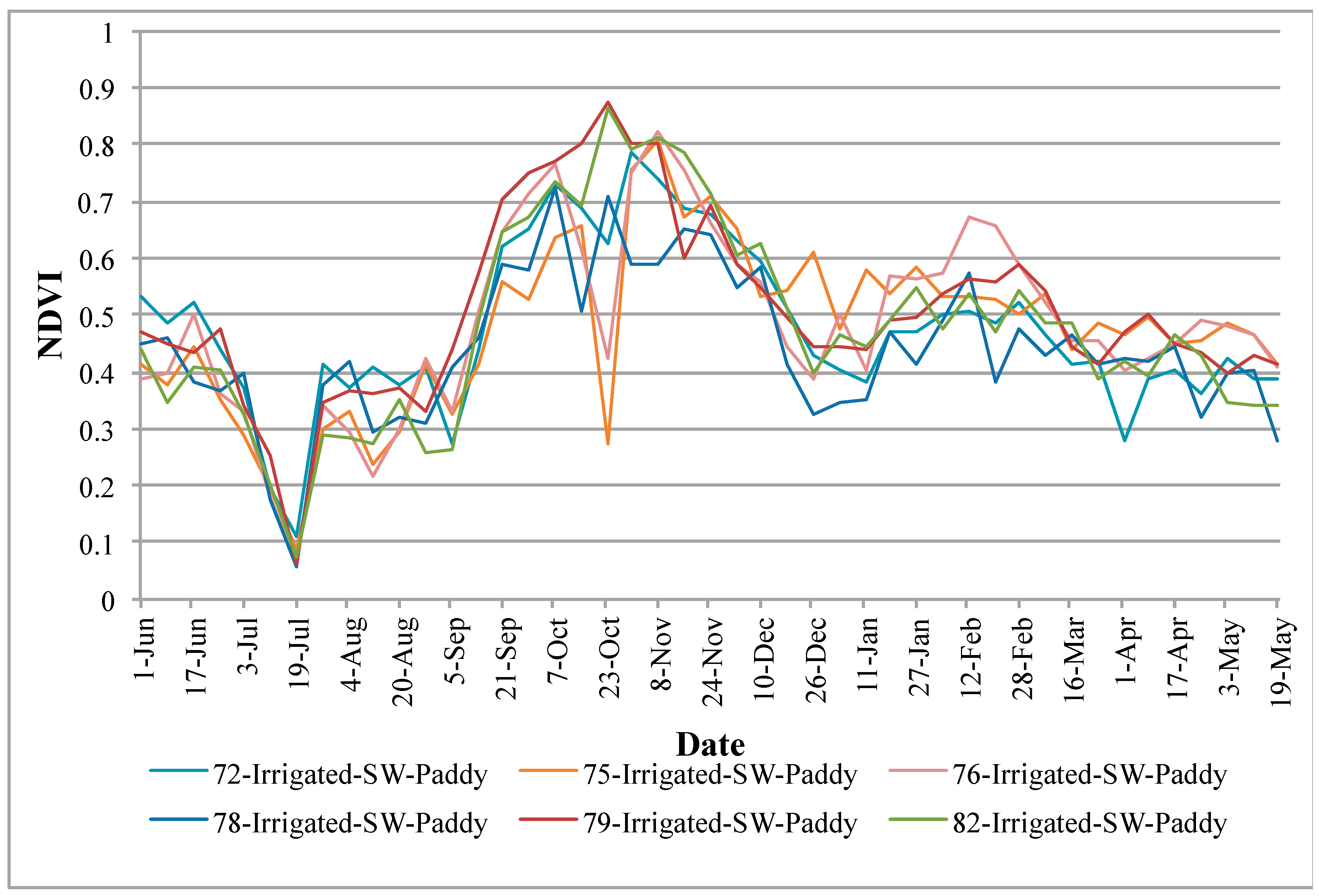
4.4. Vegetation Phenology of Various Rice Pixels from Different Zones/Regions in the Basin

Rice crop phenology was studied using NDVI time-series plots from observation points selected from land use survey data (Figure 10 and Figure 11). These NDVI time series profiles provided information on
(a)
Cropping intensities (e.g., double or single crop);
(b)
Crop calendar (i.e., when a crop begins and when it is harvested); and
(c)
Crop health and vigor (indicated by magnitude of NDVI).
Each rice class has a distinctly different phenology depicted by the NDVI magnitude and/or seasonality (Figure 10 and Figure 11). The NDVI time-series also allows the separation of short period rice and long period rice based on factors such as when a crop calendar begins, and the magnitude of NDVI.
Figure 10. NDVI time series of observed rice fields, which are classified as rice pixels in the double crop rice zone.
Remotesensing 07 08858 g010
Figure 11. NDVI time series of observed rice fields, which are classified as rice pixels in the single crop rice zone.
Remotesensing 07 08858 g011

4.5. Accuracy Assessment from Field Observations

A qualitative assessment was performed to check whether a known rice area was classified as rice or non-rice. This process was done using 91 independent observation sites (see Figure 1) where observations were conducted every 16 days during the Kharif season in 2006–2007. The error matrix (see Table 3) was constructed based on the theoretical description given by Jensen [27]. The columns of the error matrix contain the field-plot data points and the rows represent the results of the classified rice maps [28]. The error matrix is a multidimensional table in which the cells contain changes from one class to another [28,29]. Each field point is categorized as either rice or non-rice. Among the 91 ground sampling points, 44 samples were collected from rice fields in different zones with different crop calendar. The classification results show that 29 of 44 rice-sampling points (66% accuracy) were identified as rice (Table 3) and the remaining sample were identified as non-rice. There are five locations, which are identified as rice but the corresponding ground observation shows that they are from other crops such as irrigated chili, cotton, turmeric and sugarcane crops. These crops are also irrigated by surface water, which can cause high water signals ultimately making it fall into the rice category. The producer accuracy obtained for rice crop is 66% and for non-rice crop is 89%. The user accuracy for rice crop and non-rice crop are 85% and 74%, respectively. The overall accuracy for this classification is 78%. These errors are mainly the result of the MODIS 500 m × 500 m pixel size (22 hectares per pixel) and land parcels are usually relatively smaller than one pixel resulting in pixel heterogeneity of fields in the area. Also, the classification is binary, i.e., either rice or non-rice. Hence if we have a mixed class category such as rice mixed with other crops then accuracy would be expected to improve.
Table 3. Accuracy assessment using field surveyed data.
MODIS Classification
Ground ReferenceCategoryRiceNon RiceTotalProducer Accuracy
Rice29154466%
Non rice5424789%
Total345791
User Accuracy85%74%
Overall Accuracy 78%

4.6. Rice Area Fractions (RAFs)

Each rice pixel contains several different land cover classes in the study site; however, all the rice samples from the field survey, collected from different zones and used to calibrate the thresholds of our classification, have more than 80% rice area fraction. So, all the classified rice pixels are assumed to have relatively high rice fractions. Although, if the rice area fraction is not included, the resulting classified area will have overestimated rice cover. Hence, in order to reduce the potential bias caused by the rice fraction, RAF of individual pixels or its average value needs to be considered when calculating actual rice areas.
The MOD09A1 pixels have a size of approximately 22 hectares, which is larger than many individual agricultural fields of the study area. Thus, many pixels contain more than one land cover classes. Any rice classification derived from such data will provide only the full pixel area (FPA), whereas the actual rice area per pixel can be obtained only by computing sub-pixel area (SPA) [19,30,31,32], defined as:
S P A = F P A × R A F
where SPA is the sub-pixel area of rice pixel, FPA the full-pixel area of the MODIS pixel and RAF the rice area fraction. The rice area fraction, RAF = 0.8472, is derived from the 44 field survey sites distributed over the Nagarjuna Sagar canal command area (Figure 1), by measuring the areas of rice within each sample plot at each site. It is assumed that the areal composition of rice paddies over the field survey areas represents the typical sub-pixel-scale rice paddy fraction of the rice-dominant MODIS pixels for the entire study region. RAF is applied uniformly to the classified pixels to estimate actual rice area for MODIS derived rice paddy pixels for each season. The SPA of each location is computed by multiplying the FPA of that class with RAF of the class. Later, the SPAs of all samples are summed to obtain the rice area fraction from all the zones.

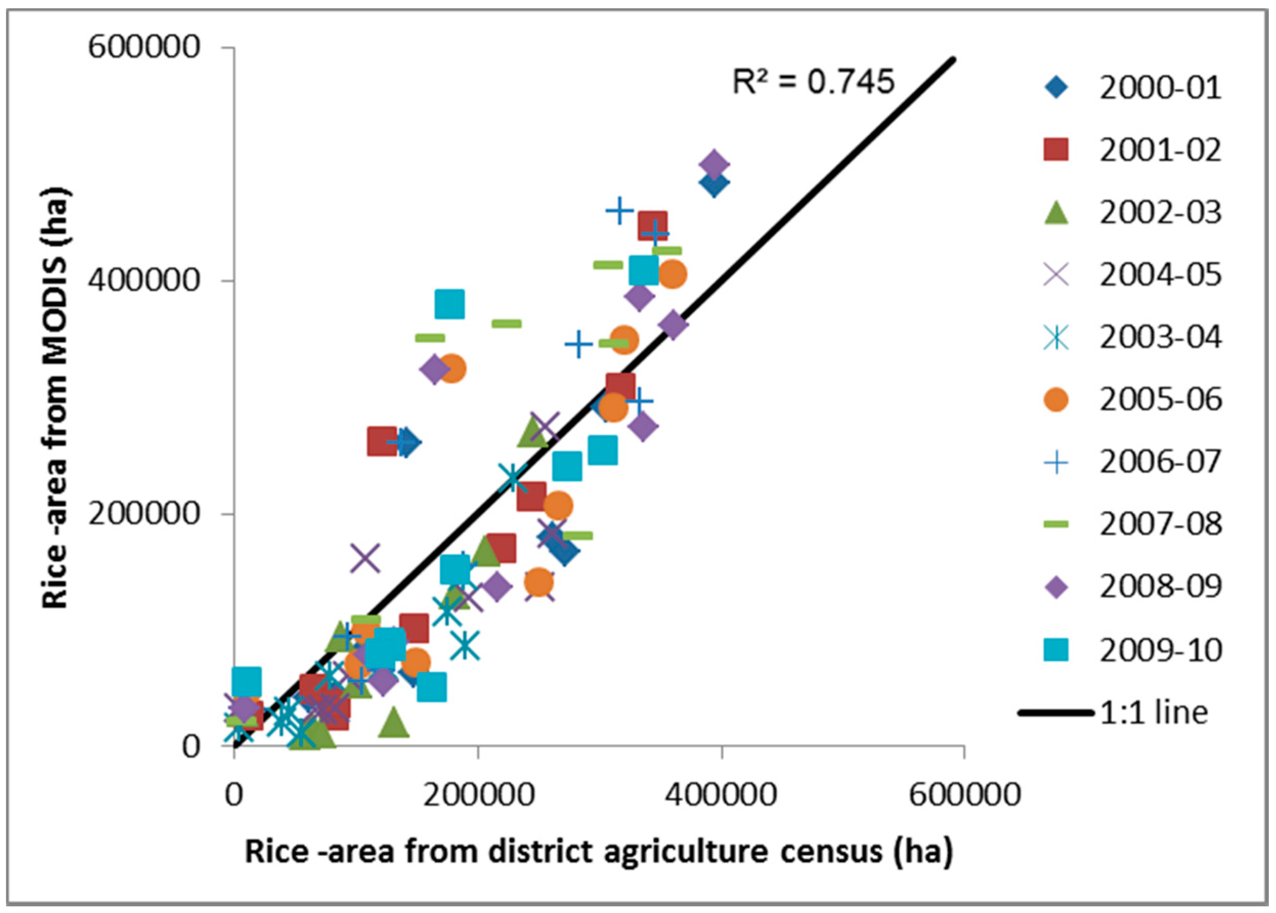
4.7. Accuracy Assessment from Agriculture Statistics

Since spatially distributed maps of Kharif or Rabi rice paddies for ground truth are not available, the agricultural statistics data from the Department of Agriculture (http://apy.dacnet.nic.in) are used to evaluate the MODIS derived rice paddy maps. To test the areal accuracy of the MODIS derived rice cropped areas, they were compared with district level agriculture statistics during the period 2000–2001 to 2009–2010. Ten districts (10 spatial units) were chosen, which are completely (not partly covered districts) covered within the extent of the study area with significant rice cropped area. District level rice cropped area were compared with MODIS derived crop area and is shown in the scatter plots (Figure 12 and Figure 13). It is obvious that there is some discrepancy between MODIS derived rice cropped area and the agriculture statistics. Therefore, further analysis of the results by statistical hypothesis significance t-test was undertaken to show whether the discrepancies can be acceptable statistically. The two groups were tested by paired-sample t-test at the level of 0.05. The results are in Table 4 showing that the MODIS derived results and the district level agriculture statistics have significant correlations except for the years 2002–2003 and 2003–2004. MODIS based estimates of rice areas during these two years are lower than the agriculture census data, which might be attributed to the over reporting of crop areas in the agriculture census data. These two years were relatively dry years when compared to others [33,34]. The total differences observed between district statistics and MODIS derived rice cropped areas from the selected 10 districts ranged from 0.2% to 24% during 2000–2001 to 2009–2010 (10 consecutive hydrological years).
The estimated RMSD of rice cropped area of the 10-districts ranged from 47,000 ha to 74,500 ha during 2000–2010, which is equivalent to 3.4% to 6.6% (Table 5) of the rice cropped area according to the district wise rice statistics. Discrepancy between the MODIS-based rice area estimates and agricultural census estimates in some administrative units can be attributed to: (1) the methods used in aggregation of rice cropped area per year from the small farm holdings and inconsistent approach and estimation methods from state to state; and (2) limitations of the 500-m resolution MODIS-based algorithm in identifying small patches of agricultural field sizes.
Figure 12. The district level comparison of rice cropped areas between agriculture census dataset and MODIS-500 m derived dataset (year wise 2000–2001 to 2009–2010). Numbers of samples are 10 districts per year and number of years are 10. Areas shown on X- and Y-axes are in hectares.
Remotesensing 07 08858 g012
Figure 13. Correlations between rice areas derived using MODIS-500 m dataset and district wise agriculture statistics (each series represents one district from 2000–2001 to 2009–2010). Numbers of samples are 10 districts per year and number of years are 10. Areas shown on X- and Y-axes are in hectares.
Remotesensing 07 08858 g013
For example, relevant to the potential issues with the agricultural census estimates (#1 above), errors in the census data of Raichur might have contributed to the particularly large discrepancy between the MODIS-derived and the census estimates (Figure 13). When the results of Raichur are excluded from evaluation, R2 of 0.745 increases to 0.841. The poorest performance of 2009–2010 results, R2 = 0.565, is also associated with the limited accuracy in Raichur. When the Raichur results are removed from the summary evaluation, R2 in 2009–2010 improves significantly from 0.565 to 0.803. Due to the large-scale irrigated rice paddies of Raichur (large double-cropping fields near the center of the Krishna River Basin in Figure 9), it is unlikely that MODIS-based estimates are more susceptible to errors in the region. Failure to account for double cropping fields potentially could have led to the large underestimation of the rice cropping areas in Raichur.
Table 4. Significance analyses between the MODIS-derived results and agriculture statistics on district scale by paired-sample t-test at the level of 0.05.
YeartThresholdSignificance
2000–20010.6413742.262Yes
2001–20020.0190642.262Yes
2002–20032.7095252.262No
2003–20043.2955482.262No
2004–20051.9680292.262Yes
2005–20060.2082692.262Yes
2006–20071.1333772.262Yes
2007–20081.3118172.262Yes
2008–20090.2208332.262Yes
2009–20100.0838922.262Yes
Table 5. Correlation between districts wise MODIS derived rice cropped areas and agriculture statistics for the selected 10 spatial units.
YearRice-Area MODIS (in ha)Rice-Area Ag. Statistics (in ha)RMSD (%)R2
2000–20011,642,6521,790,1584.30%0.752
2001–20021,641,7501,637,6563.92%0.784
2002–2003802,6261,158,4966.62%0.767
2003–2004783,9041,131,5836.00%0.693
2004–20051,069,2661,392,0695.50%0.819
2005–20062,007,7642,055,9873.47%0.695
2006–20072,200,9461,936,2173.40%0.818
2007–20081,999,0002,372,4583.93%0.681
2008–20092,180,9152,236,3443.38%0.777
2009–20101,819,7611,796,3664.66%0.565

5. Summary and Conclusions

This study demonstrates unique contrasts between the NDVI and the LSWI observed during the transplant season of rice based on ground-based spectral samples surveyed by a field spectroradiometer. Also, this study identified a new set of decision rules to map Kharif rice and Rabi rice based on land use survey. Finally, mapped flooded paddy rice for Kharif and Rabi seasons by analyzing the time series of MODIS (MOD09A1) data in the Krishna River Basin, India. Accuracy was determined by correlating MODIS-derived classification using field plot data and MODIS-derived rice areas with subnational statics obtained from the Ministry of Agriculture, Government of India. Overall a 78% of accuracy was obtained for the rice classification using field plot data and 3.4% to 6.6% of error (RMSD) observed in the MODIS derived rice area with sub national statistics over ten years.
There exist some discrepancies in MODIS derived results. We have tried to analyze the factors that might cause errors in the results. We found that clouds have a significant impact on results because all cloud contaminated pixels in the flooding and transplantation period were eliminated in the rice identifying algorithms due to their unreliability, so cloud contamination is a major source that can cause error of omission. The cloud contamination problem impacts classification, especially during Kharif season as the flooding and transplantation period of Kharif rice occurs along with monsoons. Therefore alternative datasets are needed in the regions with frequent and heavy clouds during the flooding and transplantation period. The MODIS derived results in the study have some errors due to the factors like mixed pixels caused by the coarse resolution (relative to the land parcel sizes). However, they are still useful for obtaining spatial distribution maps over a large scale and they might provide valuable information for studies such as estimation of improved evapotranspiration by accounting the open water evaporation from flooded irrigation.

Acknowledgments

The research was funded by the Australian Centre for International Agricultural Research (ACIAR) under the John All Wright Fellowship, and the ACIAR Project LWR-2007-113. The authors would like to thank the International Water Management Institute (IWMI) for providing access to the land use survey data collected during 2006–2007 and the secondary data collected from Govt Departments in India. The authors also would like to thank Venkataradha Akuraju for helping in the AILSPEX-11 and AILSPEX-12 field experiments in India. Finally, we would like to thank the four anonymous reviewers that helped improve this paper with their comments and suggestions.

Author Contributions

Pardhasaradhi Teluguntla and Dongryeol Ryu conceived the idea for this study. Preliminary work was done by these two authors. Pardhasaradhi Teluguntla extended the work and involved Biju George, Jeffrey P. Walker and Hector M. Malano in the data collection and implementation. Tables and figures that resulted from the analysis were generated by Pardhasaradhi Teluguntla and Dongryeol Ryu. The final paper was written by Pardhasaradhi Teluguntla and then sent to all authors for comments and edits. Pardhasaradhi Teluguntla and Dongryeol Ryu compiled all the edits and produced the final paper.

Conflicts of Interest

The authors declare no conflict of interest.

References

  1. FAOSTAT. FAOSTAT 2008. Available online: http://faostat.fao.org/ (accessed on 11 July 2011).
  2. Khush, G.S. What it will take to feed 5.0 billion rice consumers in 2030. Plant Mol. Biol. 2005, 59, 1–6. [Google Scholar] [CrossRef] [PubMed]
  3. Neue, H.U. Methane emission from rice fields. Bioscience 1993, 43, 466–474. [Google Scholar] [CrossRef]
  4. Denier Van Der Gon, H. Changes in CH4 emission from rice fields from 1960s to 1990s: 1. Impacts of modern rice technology. Glob. Biogeochem. Cycles 2000, 1, 61–72. [Google Scholar] [CrossRef]
  5. Wassmann, R.; Lantin, R.S.; Neue, H.U.; Buendia, L.V.; Corton, T.M.; Lu, Y. Characterization of methane emissions from rice fields in Asia. III. Mitigation options and future research needs. Nutr. Cycl. Agroecosystems 2000, 58, 23–36. [Google Scholar] [CrossRef]
  6. Belder, P.; Bouman, B.A.M.; Cabangon, R.; Guoan, L.; Quilang, E.J.P.; Yuanhua, L.; Spiertz, J.H.J.; Tuong, T.P. Effect of water-saving irrigation on rice yield and water use in typical lowland conditions in Asia. Agric. Water Manag. 2004, 65, 193–210. [Google Scholar] [CrossRef]
  7. Wisser, D.; Frolking, S.; Douglas, E.M.; Fekete, B.M.; Vörösmarty, C.J.; Schumann, A.H. Global irrigation water demand: Variability and uncertainties arising from agricultural climate data sets. Geophys. Res. Lett. 2008, 35. [Google Scholar] [CrossRef]
  8. Xiao, X.; Boles, S.; Frolking, S.; Salas, W.; Moore, B., III; Li, C.; He, L.; Zhao, R. Observation of flooding and rice transplanting of paddy rice fields at the site to landscape scales in China using VEGETATION sensor data. Int. J. Remote Sens. 2002, 23, 3009–3022. [Google Scholar] [CrossRef]
  9. Chandrasekar, K.; Sesha Sai, M.V.R.; Roy, P.S.; Dwevedi, R.S. Land Surface Water Index (LSWI) response to rainfall and NDVI using the MODSI Vegetation Index product. Int. J. Remote Sens. 2010, 31, 3987–4005. [Google Scholar] [CrossRef]
  10. Chen, D.Y.; Huang, J.F.; Jackson, T.J. Vegetation water content estimation for corn and soybeans using spectral indices derived from MODIS near- and short-wave infrared bands. Remote Sens. Environ. 2005, 98, 225–236. [Google Scholar] [CrossRef]
  11. Jackson, T.J.; Chen, D.; Cosh, M.; Li, F.; Anderson, M.; Walthall, C.; Doraiswamy, P.; Hunt, R. Vegetation water content mapping using Landsat data derived normalized difference water index for corn and soybeans. Remote Sens. Environ. 2004, 92, 475–482. [Google Scholar] [CrossRef]
  12. Xiao, X.; Boles, S.; Liu, J.; Zhuang, D.; Frolking, S.; Li, C.; Salas, W.; Moore, B., III. Mapping paddy rice agriculture in southern China using multi-temporal MODIS images. Remote Sens. Environ. 2005, 95, 480–492. [Google Scholar] [CrossRef]
  13. Xiao, X.; Boles, S.; Frolking, S.; Li, C.; Babu, J.Y.; Salas, W.; Moore, B., III. Mapping paddy rice agriculture in South and Southeast Asia using multi-temporal MODIS images. Remote Sens. Environ. 2006, 100, 95–113. [Google Scholar] [CrossRef]
  14. Sun, H.; Huang, J.; Huete, A.R.; Peng, D.; Zhang, F. Mapping paddy rice with multi-date moderate-resolution imaging spectroradiometer (MODIS) data in China. J. Zhejiang Univ. Sci. 2009, 10, 1509–1522. [Google Scholar] [CrossRef]
  15. Gumma, M.K.; Nelson, A.; Thenkabail, P.S.; Singh, A.N. Mapping rice areas of South Asia using MODIS multi temporal data. J. Appl. Remote Sens. 2011, 5. [Google Scholar] [CrossRef]
  16. Vaesen, K.; Gilliams, S.; Nackaerts, K.; Coppin, P. Ground-measured spectral signatures as indicators of ground cover and leaf area index: The case of paddy rice. Field Crops Res. 2001, 69, 13–25. [Google Scholar] [CrossRef]
  17. Ryu, D.; Teluguntla, P.; Malano, H.M.; George, B.A.; Nawarathna, B.; Radha, A. Analysis of Spectral Measurements in Paddy Rice Field: Implications for Land Use Classification. In Proceedings of the 19th International Congress on Modelling and Simulation (MODSIM), Perth, Australia, 12–16 December 2011; pp. 2009–2015.
  18. Motohka, T.; Nasahara, K.N.; Miyata, A.; Mano, M.; Tsuchida, S. Evaluation of optical satellite remote sensing for rice paddy phenology in monsoon Asia using a continuous in situ dataset. Int. J. Remote Sens. 2009, 30, 4343–4357. [Google Scholar] [CrossRef]
  19. Biggs, T.W.; Thenkabail, P.S.; Gumma, M.K.; GangadharaRao, T.P.; Turral, H. Irrigated area mapping in heterogeneous landscapes with MODIS time series, ground truth and census data, Krishna Basin, India. Int. J. Remote Sens. 2006, 27, 4245–4266. [Google Scholar] [CrossRef]
  20. Biggs, T.W.; Gaur, A.; Scott, C.A.; Thenkabail, P.S.; GangadharaRao, T.P.; Gumma, M.K.; Acharya, S.; Turral, H. Closing of the Krishna basin: Summary of research, Hydronomic zones and water accounting. In IWMI Research Report 111; International Water Management Institute: Colombo, Srilanka, 2007; p. 44. [Google Scholar]
  21. Huete, A.R.; Didan, K.; Miura, T.; Rodriguez, E.; Gao, X.; Ferreira, L. Overview of the radiometric and biophysical performance of the MODIS vegetation indices. Remote Sens. Environ. 2002, 83, 195–213. [Google Scholar] [CrossRef]
  22. Shibayama, M.; Akiyama, T. Seasonal visible, near-infrared and mid-infrared spectra of rice canopies in relation to LAI and above-ground dry phytomass. Remote Sens. Environ. 1989, 27, 119–127. [Google Scholar] [CrossRef]
  23. Ceccato, P.; Gobron, N.; Flasse, S.; Pinty, B.; Tarantola, S. Designing a spectral index to estimate vegetation water content from remote sensing data: Part 1. Theoretical approach. Remote Sens. Environ. 2002, 82, 188–197. [Google Scholar] [CrossRef]
  24. Ceccato, P.; Flasse, S.; Grégoire, J.M. Designing a spectral index to estimate vegetation water content from remote sensing data: Part 2. Validation and applications. Remote Sens. Environ. 2002, 82, 198–207. [Google Scholar] [CrossRef]
  25. Cihlar, J. Identification of contaminated pixels in AVHRR composite images for studies of land biosphere. Remote Sens. Environ. 1996, 56, 149–153. [Google Scholar] [CrossRef]
  26. Sellers, P.J.; Tucker, C.J.; Collatz, G.J.; Los, S.O.; Justice, C.O.; Dazlich, D.A.; Randall, D.A. A global 1° by 1° NDVI data set for climate studies: Part II. The generation of global fields of terrestrial biophysical parameters from the NDVI. Int. J. Remote Sens. 1994, 15, 3519–3545. [Google Scholar] [CrossRef]
  27. Jensen, J.R. Introductory Digital Image Processing: A Remote Sensing Perspective, 3rd ed.; Prentice Hall: Up-per Saddle River, NJ, USA, 2004; p. 544. [Google Scholar]
  28. Congalton, R.G. A review of assessing the accuracy of classifications of remotely sensed data. Remote Sens. Environ. 1991, 37, 35–46. [Google Scholar] [CrossRef]
  29. Congalton, R.G.; Green, K. Assessing the Accuracy of Remotely Sensed Data: Principles and Practices; CRC: London, UK, 2009. [Google Scholar]
  30. Thenkabail, P.S.; GangadharaRao, P.; Biggs, T.; Krishna, M.; Turral, H. Spectral matching techniques to determine historical land use/land cover (LULC) and irrigated areas using time-series AVHRR pathfinder datasets in the Krishna River Basin, India. Photogramm. Eng. Remote Sens. 2007, 73, 1029–1040. [Google Scholar]
  31. Thenkabail, P.S.; Biradar, C.M.; Noojipady, P.; Dheeravath, V.; Li, Y.J.; Velpuri, M.; Gumma, M.; Reddy, G.P.O.; Turral, H.; Cai, X.L.; et al. Global irrigated area map (GIAM), derived from remote sensing, for the end of the last millennium. Int. J. Remote Sens. 2009, 30, 3679–3733. [Google Scholar] [CrossRef]
  32. Gumma, M.K.; Thenkabail, P.S.; Iyyanki, M.V.; Velpuri, N.M.; GangadharaRao, T.P.; Dheeravath, V.; Biradar, C.M.; Nalan, A.S.; Gaur, A. Changes in agricultural cropland areas between a water-surplus year and water-deficit year impacting food security determined using MODIS 250 m time-series data and spectral matching techniques in the Krishna River Basin (India). Int. J. Remote Sens. 2011, 32, 3495–3520. [Google Scholar] [CrossRef]
  33. Gaur, A.; Biggs, T.W.; Gumma, M.K.; Parthasaradhi, G.; Turral, H. Water scarcity effects on equitable water distribution and land use in major irrigation projects a case study in India. J. Irrig. Drain. Eng. 2008, 134, 26–35. [Google Scholar] [CrossRef]
  34. Biggs, T.W.; Gangadhara Rao, P.; Bharati, L. Mapping agricultural responses to water supply shocks in large irrigation systems, southern India. Agric. Water Manag. 2010, 97, 924–932. [Google Scholar] [CrossRef]

