Logical Inference Framework for Experimental Design of Mechanical Characterization Procedures


1
Department of Structural Mechanics, University of Granada, 18071 Granada, Spain
2
Biosanitary Research Institute, 18016 Granada, Spain
3
MNat Scientific Unit of Excellence, University of Granada, 18071 Granada, Spain
*
Author to whom correspondence should be addressed.
Sensors 2018, 18(9), 2984; https://doi.org/10.3390/s18092984
Submission received: 18 July 2018
/
Revised: 28 August 2018
/
Accepted: 1 September 2018
/
Published: 7 September 2018
(This article belongs to the Special Issue Ultrasonic Sensors 2018)
Abstract
:Optimizing an experimental design is a complex task when a model is required for indirect reconstruction of physical parameters from the sensor readings. In this work, a formulation is proposed to unify the probabilistic reconstruction of mechanical parameters and an optimization problem. An information-theoretic framework combined with a new metric of information density is formulated providing several comparative advantages: (i) a straightforward way to extend the formulation to incorporate additional concurrent models, as well as new unknowns such as experimental design parameters in a probabilistic way; (ii) the model causality required by Bayes’ theorem is overridden, allowing generalization of contingent models; and (iii) a simpler formulation that avoids the characteristic complex denominator of Bayes’ theorem when reconstructing model parameters. The first step allows the solving of multiple-model reconstructions. Further extensions could be easily extracted, such as robust model reconstruction, or adding alternative dimensions to the problem to accommodate future needs.
1. Introduction
Inverse problems are used in various fields, including medical imaging, nondestructive testing, mathematical finance, astronomy, geophysics, or sub-surface prospecting, whenever interrogating phenomena or properties of a system that cannot be readily quantified. The inverse problem can be defined in opposition to the forward problem. Given a physical system, the forward problem consists of using an idealized model of that system to predict the outcome of possible experiments. In contrast, the inverse problem is posed to interrogate or reconstruct an unknown part of the system given an observed set of output data.
This reconstruction problem was historically first solved in a deterministic way, providing a unique answer to the unknown parameters [1,2,3]. However, if the degree of certainty and reliability of the parameters is relevant, a probabilistic approach is required. This was introduced using the framework of Bayesian statistics by Cox and Jaynes [4] based on Cox’s postulates [5], and still being developed [6,7,8,9,10,11,12,13]. Its central idea is that the unknown is defined as a probability density function over the model parameters to be reconstructed, and this probability is updated with the experimental information and linked with a model through Bayes’ theorem. An alternative theoretical framework was posed by Tarantola [14] based on the idea of conjunction of states of information (theoretical, experimental, and prior information, generally on model parameters). The axioms of probability theory apply to different situations: the Bayesian perspective is the traditional statistical analysis of random phenomena, whereas the information states criterion is the description of (more or less) subjective states of information on a system. However, the collection of applications successfully solved by Ensemble Kalman Filter-type algorithms (EnKF) are not directly solvable by the proposed formulation, at least without profound adaptations.
Furthermore, its delicate formulation poses difficulties when modifying and extending it to solve real-world needs. To overcome this, we propose an information-theoretic reconstruction framework, which is built on a new metric of information density that drops Cox’s normalization in favor of simplifications. This metric is used with the concept of combining information density functions from two independent sources: (i) experimental measurements and (ii) mathematical models, over the same data (observations and model parameters) with the aim of finding which ones are all plausible at the same time. This new framework ultimately allows the straightforward solving of problems combining multiple concurrent models, or conveniently solve as experimental design, sensor design and placement problems in specific cases as in the ultrasonics testing in a probabilistic way, which only recently has been computed from the Bayesian perspective [15,16,17,18]. Beyond this, new dimensions can be defined into the problem to accommodate future needs. Moreover, models are not required to be causal, paving the way to contingent models such as stochastic associations, for instance, whose scope extends to applications such as image reconstruction, face recognition or complex physics-based model parameters reconstruction.
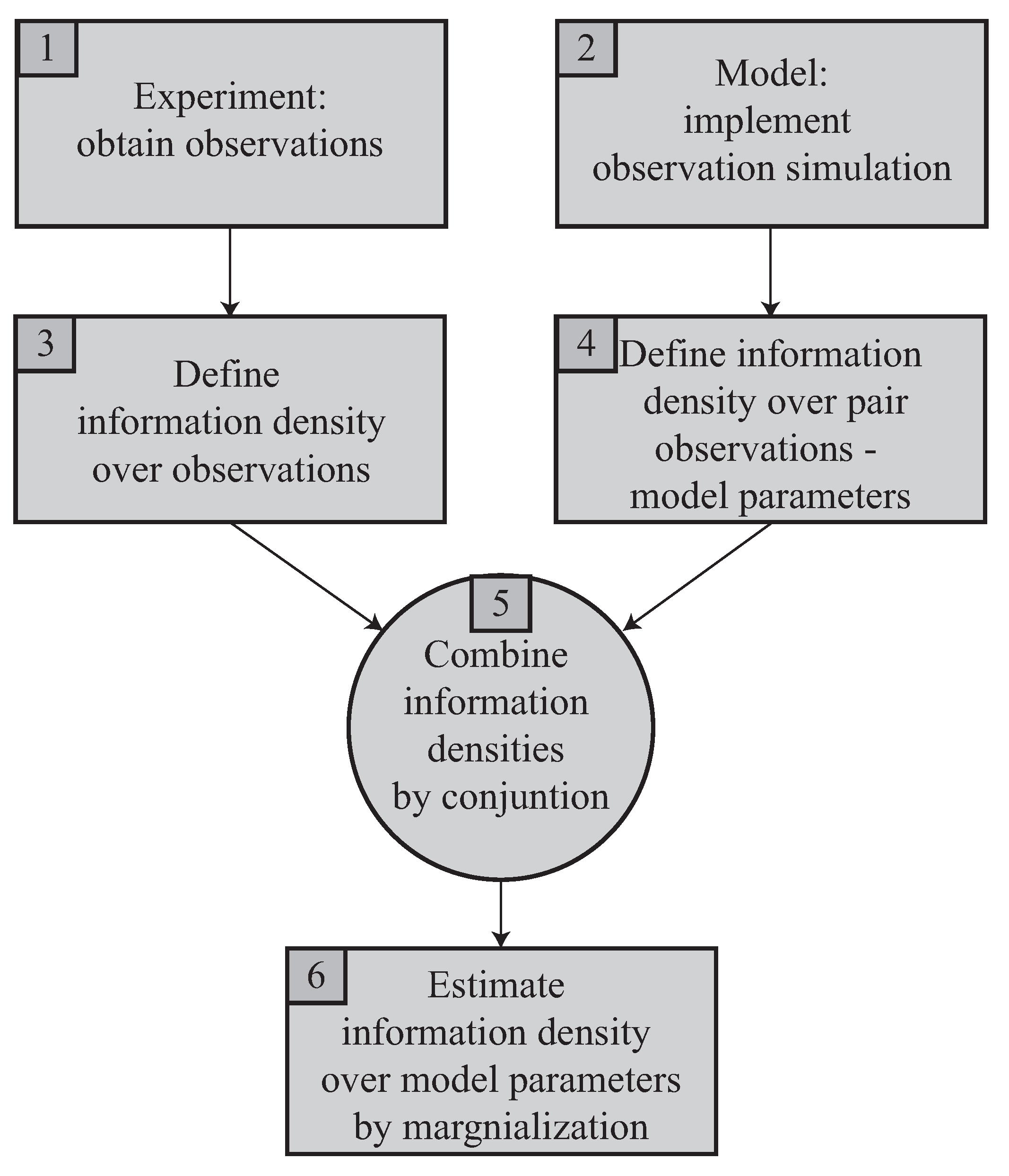
The next section details and formalizes the procedure to solve the problem, whose components are reorganized and outlined in Figure 1.
As follows. The two mentioned starting ingredients at the top are an experiment performed to capture some measurements, in box 1, and, in box 2, an idealization of the experimental system made throughout a model, which allows simulation of the measurements, but depends on the model parameters, which are the unknowns of the problem. In box 3, to treat the observations from box 1 in an uncertain way, they are described by means of the concept of information density over the theoretically possible space of observations, formally defined in Section 2.1 and Section 2.2. In box 4, the pairs of values of sought model parameters and simulated observations are analogously defined by means of their joint information density. In box 5, both sources of information, experiment and model, are combined as described in Section 2.2. In box 6, the probabilistic reconstruction answer is yielded as described in Section 2.4.
This scheme solves the basic form of the reconstruction inverse problem, assuming a single model and a predetermined way of measuring. However, the formulation proposed below has the strength of being easily extended to solve practical problems explained in Section 2.3, where the former assumptions need not be made.
In this work we propose a new technique to optimize the experimental design of a testing system or sensor and illustrate it for the particular case of characterizing a viscoelastic material, step by step. First, the information-theoretic inverse problem framework is formulated, then, the practical method is detailed describing the process of parametrization, the operation with discrete observation data or signals, and two key extensions: to hypothesis testing and to experimental design optimization. The proposal is illustrated with a practical example to reconstruct a mechanical model from a tensile testing.
2. Theory
2.1. Definition of Basic Variables
Assuming that the two sources of information are the experimental observations and an idealized model that simulates observations for given model parameters, two basic variables stem from this premise: observations and model parameters.
The observations are, in the most general case, vectors compounding a set of signals , but may also be a single signal, analog or digitally sampled, sets of values, or even a single measurement value. Although a unique space of observations can be defined to contain all possible observations, depending on their origin they can be either observed or modeled . Examples of observations may be ultrasonic or seismic recorded signals, optical, X-ray or thermographic images, or any measurement based on any physical magnitude used to interrogate the system under study.
The model parameters are analogously a set of diverse physical parameters, which define a manifold . They are the input of the mathematical model that simulates the experimental behavior and its measurable by an output. They may stand for damage parameters, pathology or sought mechanical properties, for instance, that feed models that simulate the observations described above. In the numerical example in Section 4, combining three sources of information is tested: model-based forecast, observation, and experimental design parameters for its optimization.
2.2. Definition of Information Density and Its Operations
To treat this data and in an uncertain way, we do not define univocal values, but information densities over them. The information density over either of them (x for generality) is defined from the conception of Cox [5] as a degree of belief or certainty that the values of x are plausible. Therefore, the probabilities that are established as a consequence of this logical framework are objective and the logical relations in that axiomatization [19,20]. They can be understood as states of knowledge, in contrast to the physical propensity of a phenomenon. A more detailed discussion is provided in [21]. The present definition of information density is compatible with either the evidential, logical and even subjective theoretical frameworks described in [21].
In particular, we formally define the information density of an event or value x as a nonnegative real that is zero () when its value is impossible, and the larger the more plausible. Two logical inference operations introduce a structure to the space of all probability distributions. Starting from the and and or operator definition for Boolean logic (which can adopt the values of true or false, without intermediate degrees of certainty), over two probability distributions and that may represent two different sources of information a and b about the same events,
the simplest logical operations over information densities f that fulfill these axioms are,
| false | false | false | false |
| false | true | false | true |
| true | false | false | true |
| true | true | true | true |
Note that the normalization requirement of either Kolmogorov axioms or Cox’s postulates (Kolmogorov axioms state that the probability P of any events A, B satisfy [22],
- Non-negativity: .
- Finite additivity: .
- Normalization: .)
is not imposed here, which will strongly simplify the formulation, as shown later. In particular, dropping the normalization axiom in the definition of the information density f simplifies the final formulation in comparison with the Bayesian inverse problem as well as theory of Tarantola.
A main cornerstone of this formulation is that the relationship between the model parameters and the observations provided by a model need not to be an implication due to a cause-effect, which requires to define the conditional probability of Bayesian statistics. Instead, just the conjunction of information densities needs to be defined, in which the causality between model and observations may be inverted or even not exist, as further discussed in [21]. These two characteristics define the relationship between model and observation. One uses probability as logic, and alternative one interprets it as information content. They will be shown below to allow the solving of reconstruction problems with multiple concurrent models, also paving the way to contingent models such as stochastic associations, as well as experimental design and placement problems, in a simple and straightforward way, both conceptually and computationally.
Therefore, we define the information contents that come from the observations as , and that provided by the model as , in the sense that the model couples values of model parameters with observations , yielding degrees of certainty f when the fed values in the model is fulfilled or not with a range of degrees of plausibility.
The origin of the uncertainties is, therefore, incorporated into the interpretation of probability as a measure of relative plausibility of the various possibilities obtained from the available information. This interpretation is not well known in the engineering community where there is a wide-spread belief that probability only applies to aleatory uncertainty (inherent randomness in nature) and not to epistemic uncertainty (missing information). Jaynes [4] noted that the assumption of inherent randomness is an example of what he called the Mind-Projection Fallacy: our uncertainty is ascribed to an inherent property of nature, or, more generally, our models of reality are confused with reality.
The interpretation of the final inferred model probability can be used either to identify a set of plausible values, or to find the most probable one (expected, i.e., that with maximal information density, argmax ), or, following Tarantola [14], just to falsify inconsistent models (those with low f), since according to Poppers falsationism [23], that is the only thing we can assert.
2.3. Definition of Extended Variables
The first extension that this framework allows is the case when several models can be combined. The model forecast may therefore also depend on the hypothesis we assume about the model physics, which in turn implies distinct sets of model parameters for each hypothesis. This brings in the hypothesis within a set (which is usually a discrete manifold, but not necessarily) as a new uncertain variable, which conditions the number of unknowns and therefore the model complexity. For instance, decisions can be made on whether some model parameters are known from literature or treated as unknowns to be sought. Alternatively, models can be added or removed in hierarchical combinations (for instance as multiscale models) or in parallel, as illustrated and clarified in the numerical example at the end of this work.
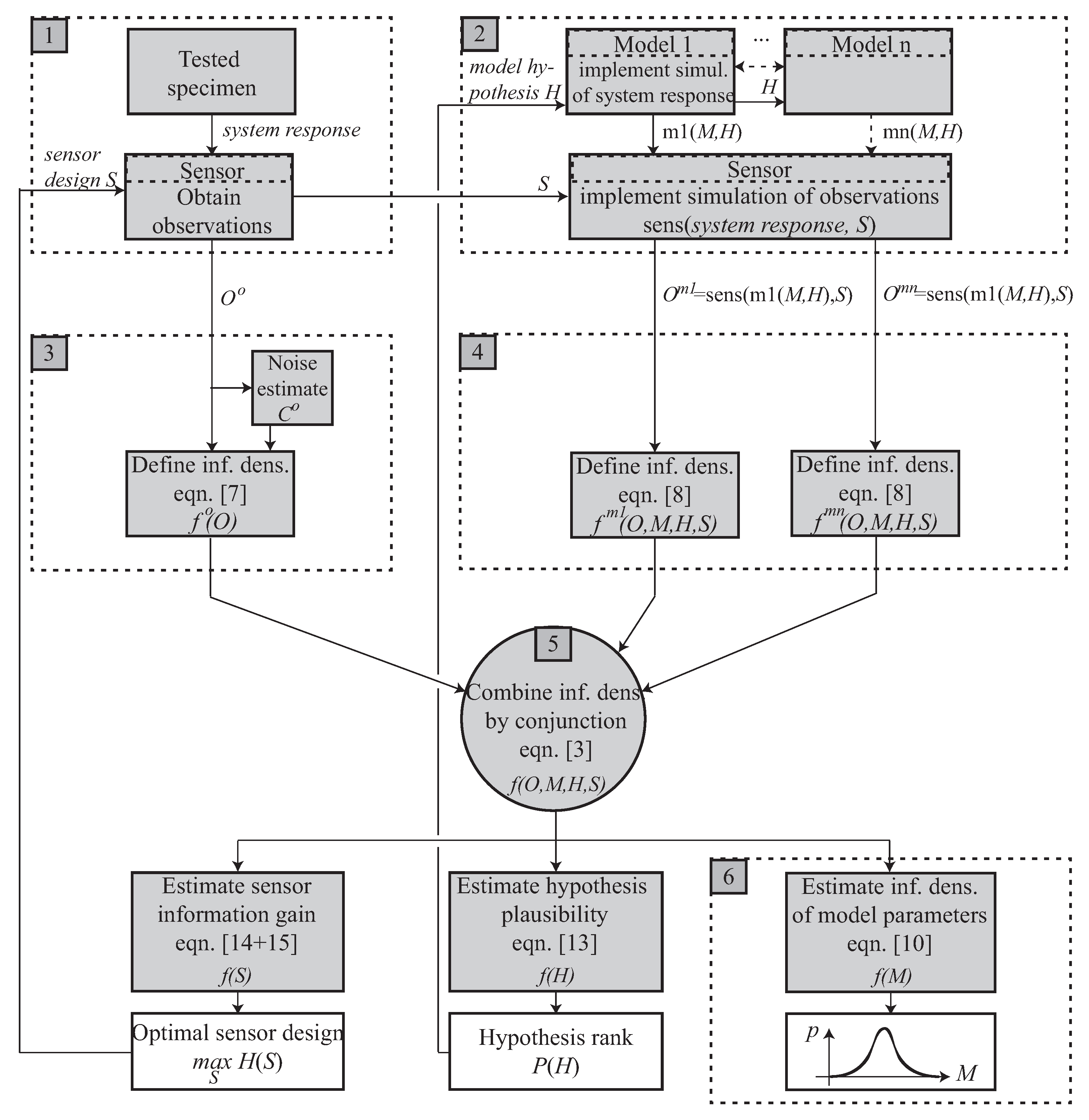
This extension to consider several hypotheses on the model or models is included in box 2 of the flow chart in Figure 2 by multiplying the possible models and making them dependent on the hypothesis .
On the other hand, in real practice, the way the system is interrogated must be decided. This implies a problem of sensor optimization and even in experiments for large-scale [24,25,26,27], in the wide sense of sensors, either as positioning, their internal design, any measurement filtering or signal processing aimed at extracting the signal parts with most useful information while minimal noise, or the measurement domains (time, frequency, phase, cepstrum, etc.). This gives rise to a set of sensor parameters within a manifold of possible values , which become the variables to optimize. The sensor placement optimization procedure will be described and illustrated in detail in a future work.
This extension to consider the design of the interrogation system is included in boxes 1 and 2 of the flow chart in Figure 2 by splitting the experiment into the system and the sensor that captures its response, which depends on the experimental design parameters .
Both and are analogously defined in a probabilistic sense by means of information densities defined over their spaces and , yielding the information contents provided by the observations as , and those provided by each concurrent model n as , or, in the case of a single model, just .
Analogously to the extension to and , further dimensions could be easily extended to the formulation, to accommodate future needs.
2.4. Information Theory Inverse Problem
Recall the flow chart in Figure 1 and focus on the concept of information density functions f, which are combined using the logical and operator [21,28,29]. Then, we have two or more sources of information (probabilistic propositions) to infer information about the model parameters . We introduce, i) a source from experimental observations of the system , and ii) a source from a mathematical model of the system , in this case, the probabilistic logic conjunction operator allows computation of the information state that the system parameters fulfill both propositions simultaneously, , as,
Note that the simultaneity of the propositions relieves the causality requirement of the Bayesian framework. Following the basics of the scientific method for physical sciences, hypotheses are proposed that explain the observations, which, in our case, are materialized as models that try to be predictive. The next step is the hypothesis validation by confronting those predictions against the observations, which is here formulated with the aim of partial degrees of certainty as the conjunction of certainty of predictions being true at the same time as observations. This is parallel and therefore consistent with hypothesis testing.
In addition, multiple models can be combined, following Figure 2. If several models (, , …) provide information, the joint information can be generalized as,
Note that these models may possibly relate different subsets of model parameters, or just represent competing hypothesized imperfect models relating the same parameters in an attempt to make robust predictions in the case none of the available models perfectly predict observations.
Assuming that the experimental information on observations is carried out with sensors that are independent of techniques to infer experimental information on model parameters, and the same is true for model hypothesis and experimental designs, the joint density can be split as the product . Note that is the noninformative density function or constant. This is not true for the model information , since it relates observations and model. In the case of the observational world, as opposed to the simulations, superscripted by m, which usually is no information (noninformative uniform distribution). However, depending on the experimental design, the observations may be of different size or even nature (for instance measuring at different points or even measuring velocities instead of displacements, for instance), which makes dependent on S in the sense that the structure of O changes, but not that the information density on S modifies the information density on O.
The reconstructed probability for the model parameters providing the model hypothesis and experimental design is obtained from the joint probability in Equation (3) by extracting the marginal probability for all possible observations and provided the model hypothesis is assumed to be true () and one experimental design as,
where is a normalization constant that replaces the dropped model hypothesis probability, which can be removed since f is unscaled. Note that here, ’marginal probability’ is defined in the loose sense of dropping the scaling. The assumption of no prior knowledge about the model parameters is represented by the noninformative distribution, i.e., an arbitrary constant in the assumed case of Jeffrey’s parameters , leaving,
3. Method
3.1. Model Parametrization
The mathematical model of the experimental system maps a set of model parameters to simulated observations , following some idealizations, in turn based on some hypothesis and interrogation system design . Note that this mapping can range from a cause-effect physical relationship to just a contingent stochastic association.
The present inverse problem formulation requires that the model parameters are of Jeffrey’s type, which have the characteristic of being positive and as popular as their inverses [14]. If parameters are of Jeffrey’s type, the present formulation can be shown to be equivalent to the Bayesian framework except for a constant, which is detailed later in Section 3.6. The benefits are that all noninformative densities are constant and therefore dropped from the formulation. This assumption is required for the definition above of the logical operators and , as well as for defining noninformative densities as constants to be fully correct.
Many model parameters are non-Jeffreys, which is evident in the following example. If two materials with different elasticities (for instance of twice Young’s modulus) are compared in terms of their stiffness and compliance (its inverse), different distances are obtained. Since there is no reason to prefer one over the other, the definition of their distance should be independent of the choice, which can be attained through a logarithmic change of variable [30,31]. This change of variables is completed with a mapping from to a predefined range of physically reasonable values , to improve numerical stability, as,
3.2. Particularization for Set of Discrete Observations with Gaussian Uncertainties
Observations are usually assumed to follow a Gaussian distribution whose mean is that of the experimental observations and whose covariance matrix quantifies the measurement error noise [32,33,34]. Likewise, the numerical errors from model m may also be assumed Gaussian centered at the numerically computed ones , where is the m-dimensional mean vector of , with covariance matrix . However, the numerical errors are oftentimes negligible compared to the experimental ones. The density fulfilling both propositions and is similar with the likelihood density under Gaussian assumption with .
Recall that the observations are a discrete vector , , and that the assumptions made above are valid for every sample i. In addition, considering the compound probability of the information of the sensors and all instants of time is the product of each one individually, it supposes independence of information, and this product is equivalent to a sum within the exponential and the Gaussian distribution that allows an explicit expression of probability densities,
The term corresponds to a misfit function between model and observations,
The mode criterion can be adopted as it finds the most probable model parameter. Finally, if classical probability densities are desired, the constant is derived by imposing the theorem of total probability since the latter is defined by normalization to 1 as,
3.3. Extension to Model Hypothesis Selection
As introduced above, the probabilistic nature of the reconstruction is partly motivated by the fact that the model itself may not necessarily reproduce or fully explain the experimental setup. If several models (or hypothesis within the model) are candidates based on different hypothesis about the system, the previous probabilistic formulation of the inverse problem also provides information to rank them. The underlying idea is the following: if the model hypothesis is considered to be an uncertain discrete variable, its probability can eventually be extracted as a marginal probability from Equation (3). The probability of each hypothesis will therefore have the sense of degree of certainty of being true in the sense that the probabilistic conjunction of certainty (or information) provided by the experimental measurements and model are coherent [9,11].
The goal is to find the probability , understood as a measure of plausibility of a model hypothesis [13], or in other words, the information gain it provides, or how much can be learned by using the hypothesized model. It is simply derived as the marginal probability of the posterior probability defined in Equation (3),
If no prior information is provided by the user about the hypothesis then . Furthermore, this procedure involves the same integral as that for the constant , i.e., allowing to reuse the integral defined in Equation (11),
where the normalization constant comes from grouping previous constants that multiply and it can be solved from the theorem of total probability over all hypothesis to obtain probabilities, .
Note that multiple dimensions of the problem can be coupled to try to solve problems such as robust parameter reconstruction [35], for instance, or others defined in future needs. The procedure for robust parameter reconstruction would imply a first step where the hypothesis plausibility is computed using Equation (13), followed by a second step where the model parameters plausibility is computed using an alternative derivation of Equation (5) without restricting to a particular hypothesis , but rather incorporating all of them, by,
Note that the space of hypothesis is discrete, so rather than integrating over it, a sum is formulated.
3.4. Extension to Interrogation System Design
Recall that by interrogation system design, we may understand any mapping from experimental output to recorded signals, which may range from experimental design parameters, the positioning of the sensors, any measurement filtering aimed at extracting the signal parts with most useful information while minimal noise, or the measurement domains (time, frequency, phase, cepstrum, etc.), with the same goal.
This goal is formulated as finding the that maximizes the information density . It may be more useful to understand it as maximizing the information entropy , which is a measure of the information contents [36]. The information density is again derived as the marginal probability of the posterior probability defined in Equation (3), assuming no prior information about the sensors nor model parameters,
and can be interpreted as the information gain or a measure of what can be learned for every value of . Instead, the information theory community typically operates with information entropy (measured in bits, nits or hartleys depending on whether the log base is 2, e or 10) which is readily obtained from the probability, which in turn comes from normalizing the information density to fulfill the theorem of total probability,
If a reliability or cost of failure related criterion is preferred for the sensor optimization, the probability curve should be computed instead of the entropy, since is directly related to the reliability , whereas the cost efficiency can be attained by estimating the total probabilistic cost as the sum of the cost of sensors, that may depend on their configuration and number , and the cost of failure, which in turn depends on .
3.5. Summary of Extended Framework
The variables and equations described above are organized in the flow-chart in Figure 2, which details the concepts outlined in Figure 1, where the extensions are clearly marked. It starts from the ingredients at the top and yields the answers at the bottom, from left to right.
In particular, note that, beyond the standard inverse problem goal of estimating the model parameters (box 6), the framework delivers (i) the sensor information gain depending on its design, which allows optimization of the experimental design or placement, and (ii) the plausibility of alternative model hypothesis, which allows ranking and choosing among plausible mathematical idealizations of the physical system. In addition, note that multiple models may be concurrently adopted (unfolding of box 2), which provides practical solutions where multimodal, multiscale or multiphysics are relevant.
3.6. Validation
A simple procedure to validate the provided formulation is to compare the model reconstruction Equation (3) and the hypothesis ranking Equation (13) with those obtained using the Bayesian framework by Beck [9,37],
where stands for the data, the model parameters, the model class, and is the prior on the model parameters [14], respectively. Note that all formulations imply the same computations except for a computationally expensive constant, whose computation is typically omitted and adjusted using the theorem of total probability, which coincides exactly with the proposed procedure when extended to computing the posterior probability p by normalizing the information contents f. The computation of the integral is here avoided for the model parameter reconstruction, and only needed for hypothesis testing and experimental design optimization. The Bayesian concepts used in this study requires Jeffrey’s type parameter, which is obtained through a logarithmic mapping, and is used combining a priori information from two independent sources over the observations and model parameters, to find the plausibility of them simultaneously.
4. Example
To illustrate the utility and effectiveness of the proposed method, a simple but nontrivial inverse problem is solved. It consists of a tensile test where the sensor is a generic displacement sensor characterized by its measurement error. The requested results are the constitutive nonlinear viscoelastic mechanical constants of a quasi-incompressible soft tissue sample. However, the extended formulation allows the easy ranking of the plausibility of several models detailed below, as well as optimizing the interrogation system, also detailed later.
The following constitutive laws are hypothesized:
- :
- Maxwell viscoelasticity that additively combines strains from damper of viscosity and nonlinear elastic spring described by shear modulus and nonlinearity of first order Landau-type , which relates shear stress and strain , with parameters constants being the output of the model governed by,The strain is defined in the models depending on the constitutive assumption considered as, , and , or linear elastic strain, nonlinear elastic strain, and viscoelastic strain, respectively. Note that is the strain tensor the subscript e.g., is referred to linear, nonlinear, or viscoelastic part, respectively. This consideration is defined in the constitutive equation that is useful to establish the different model hypothesis.
- :
- Maxwell linear viscoelastic, with parameters constants ,
- :
- Linear elastic, with parameters constants ,
- :
- Maxwell viscoelasticity with third order nonlinear elasticity, parameters constants governed by,
- :
- model combined with a second phenomenological model that states that as dynamic viscosity where t is time in seconds.
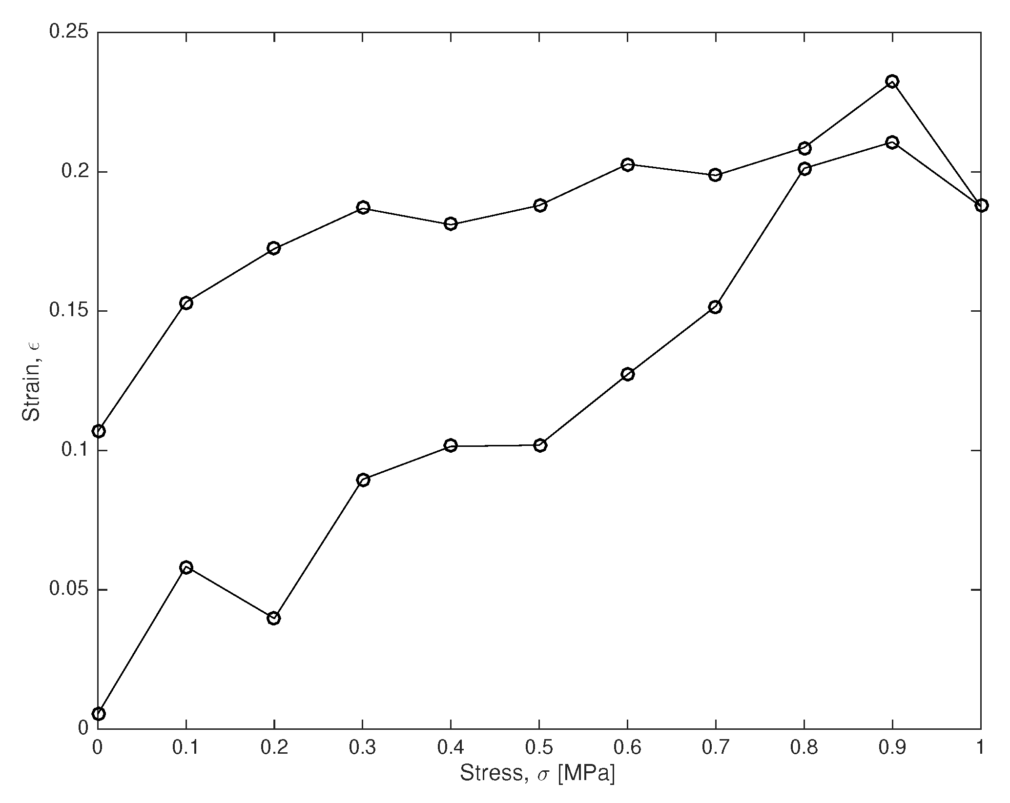
The test is defined as a stress-controlled loading and unloading test at constant velocity between 0 and 1 [MPa] and duration [s]. It yields the simulated stress-strain curve in Figure 3, where measurements are taken every s.
To validate the capability of the method under fully controlled uncertainties, instead of real data, the experiment was simulated from model with [MPa], [MPa·s] and [kPa], by adding Gaussian noise simulated with a significative standard deviation of 10 [kPa].
The probabilistic inversion is carried out by joining the experimental information from the experimental stress-strain curves with the models above.
4.1. Model Parameters Reconstruction
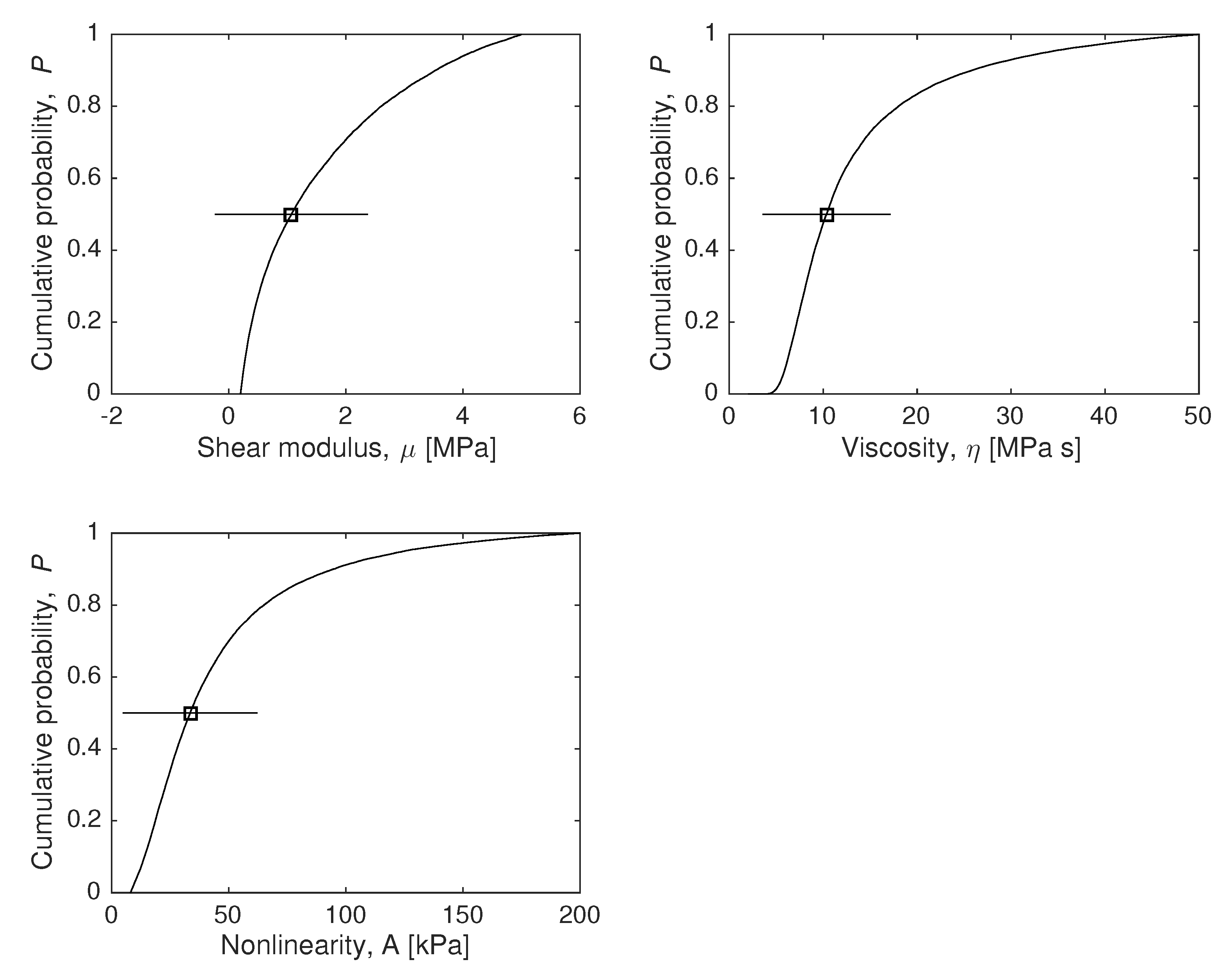
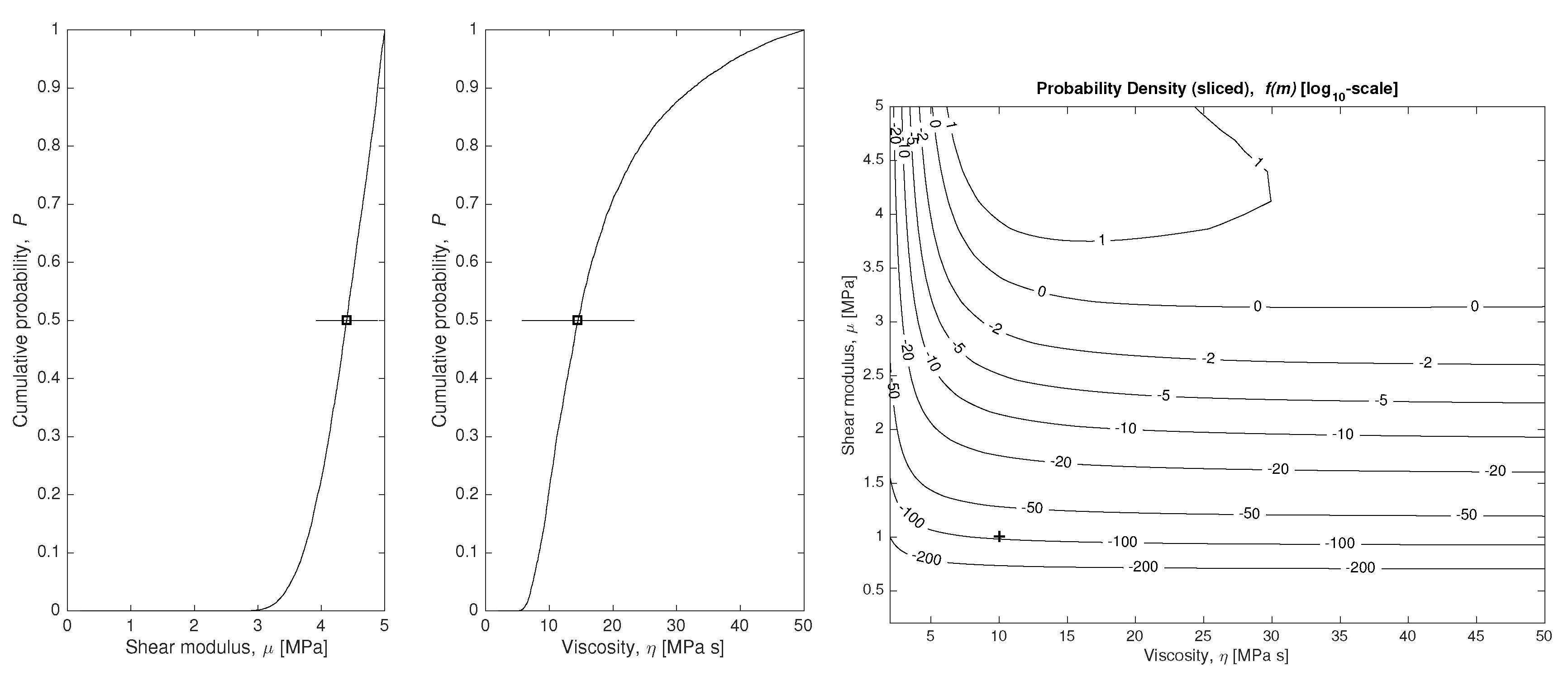
To answer the question of how much we can know about the values of the constitutive constants , under hypothesis , the marginal probability density can be computed using Equations (10) (a continuous formulation is introduced using integrals) and (21). because in this example, the time dimension is discretized, which forces the use of Monte-Carlo approximation. The results are shown in Figure 4.
The integral in Equation (11) is approximated computationally by a standard Monte Carlo sampling, which approximates the integral of any integrand that depends on the parameters x over a parameter subspace using,
where the integrand is evaluated at N random points called samples. The precision is controlled by the number of samples, here chosen as points, which takes a few seconds on a laptop. Note that, in each hypothesis, the physical parameters that are not present in the formulation are not assigned value zero, but rather not assigned any preferential information density. In other words, this is equivalent to assigning the noninformative (constant) information density over the non-used models’ parameters. When numerically solving the problem, such parameters are actually never assigned any value. The integral is only performed at the computation of the model-class selection.
Considering that we only have 21 experimental data (21 circles in Figure 3) with a significative simulated measurement error (10% Gaussian noise on each data), all parameters are successfully estimated (squares with error bars on each plot of Figure 4), as well as their certainty and the shape of the distribution function.
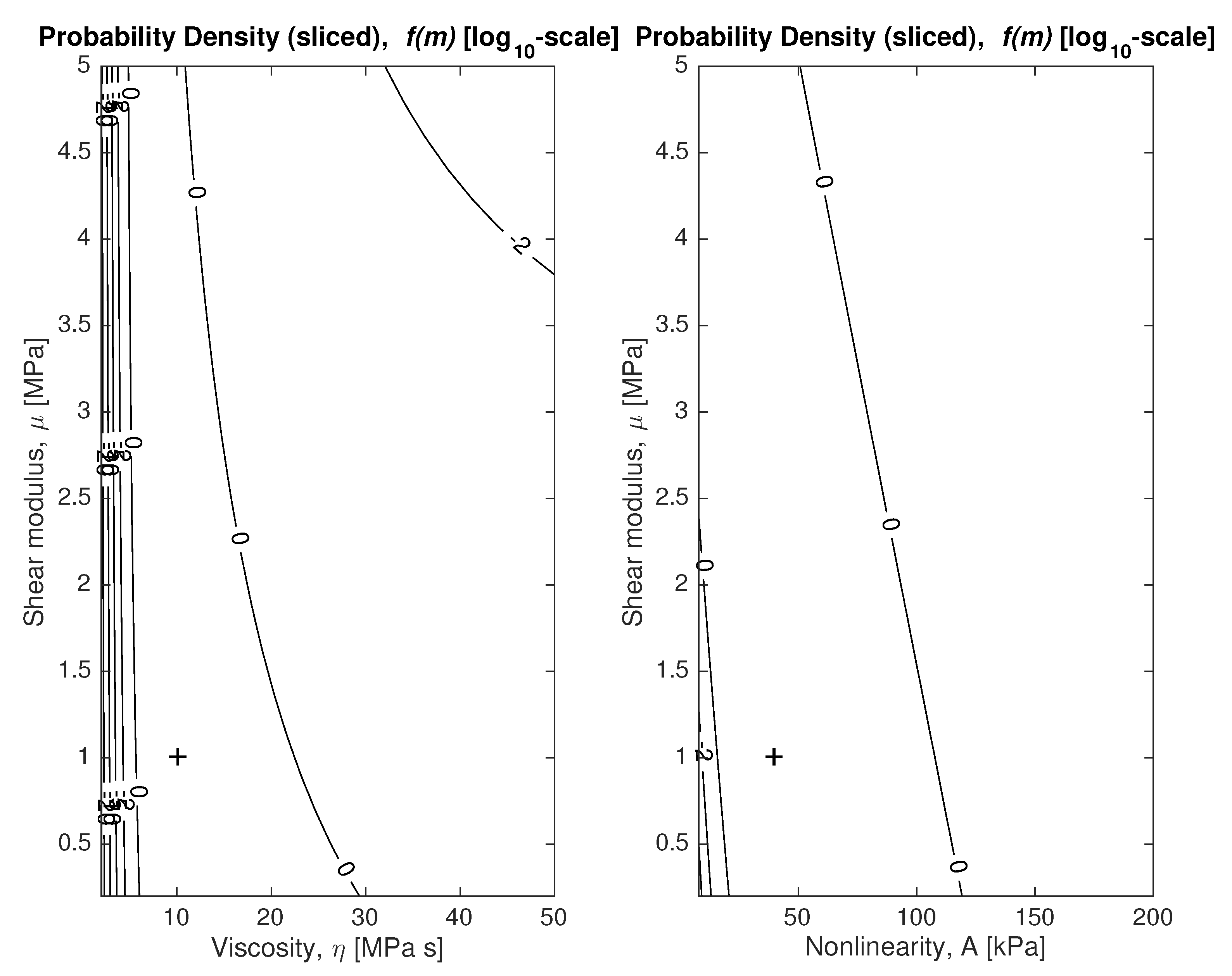
To answer the question of how coupled or entangled the unknown model parameters are, visualizing the plausibility maps, which is a function, would require a 4-dimensional plot. Instead, we slice it in two 2D contour plots. The slices mean that the model parameters are evaluated by moving two and by fixing the remaining parameters at the most probable values. The contour plots are shown in Figure 5, where the optimal viscosity parameter is 10 [MPa · s] and it is marked with a plus sign in the plot.
Note that the figure on the right reveals a strong correlation between the linear and nonlinear shear moduli (usually considered in biomechanical characterization [38]), which is a factor for the ill-conditioning of the inverse problem.
4.2. Model Hypothesis Ranking
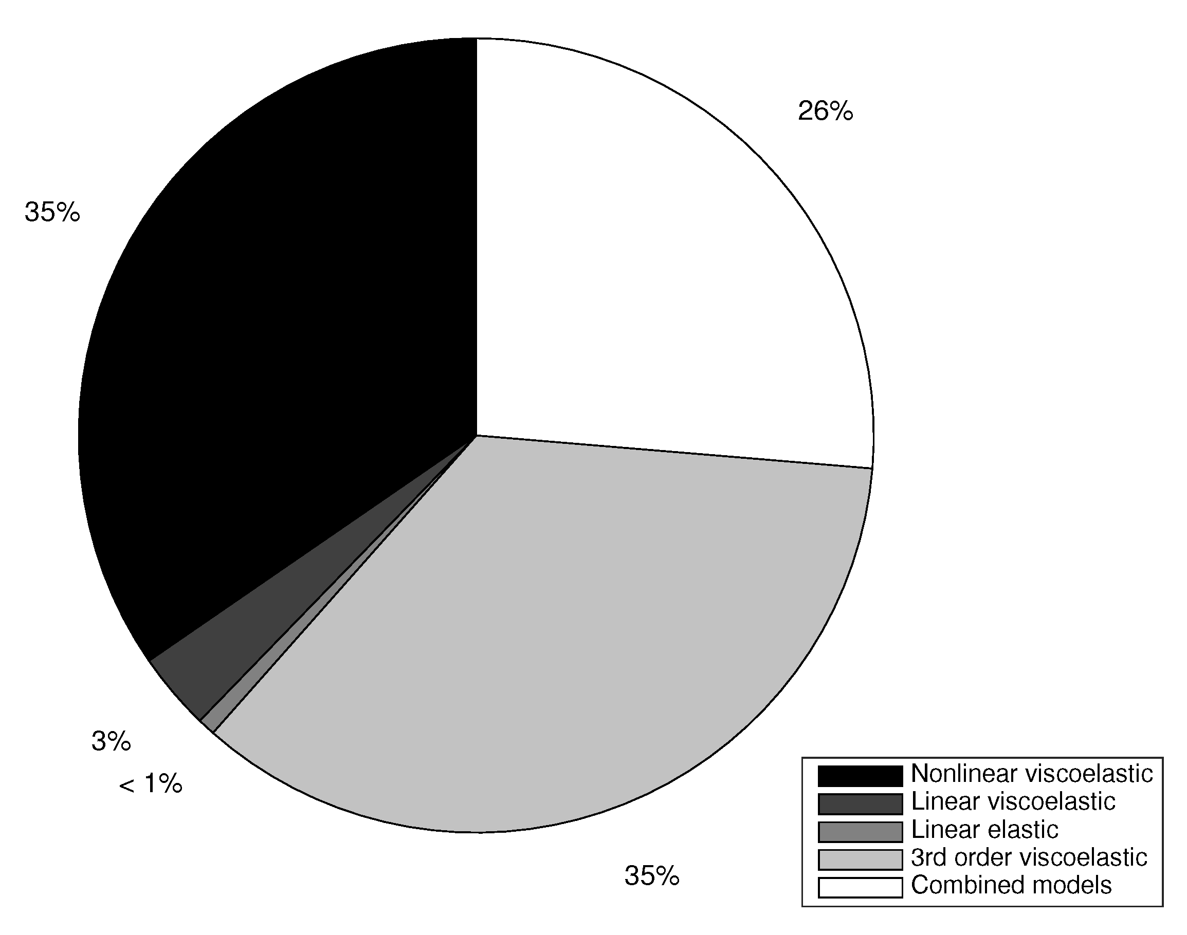
To answer the question of how much we can trust the assumed physics among a set of candidates, or which model complexity is best by assuming known or unknown physical constants, the model hypothesis raking of the five hypothesis described above is computed using Equations (13) and (21) in Figure 6.
For clarity, the degrees of hypothesis reliability is presented in % by rescaling the information density from Equation (13) as,
As an example, the reconstruction of the nonlinear experimental data using the model and the corresponding plausibility map contour plots are shown in Figure 7,
Note that the reconstructed parameters are distant from the ones used for the simulation, which is to be expected. The badness of the fitting is also quantified by its low plausibility shown in the ranking in Figure 6.
4.3. Interrogation System Optimization
Finally, the problem of sensor optimization is illustrated by solving the optimal testing duration , within a search range s. Despite the CPU time for solving this low-dimensional problem is quite small, in large-dimensional problems the computational time is expected to be large, and scalability should be studied carefully. The entropy H is computed using Equations (16) and (21) and yields the optimal testing configuration using duration [s], as shown in Figure 8 sensor information gain dependence on its design.
The case where some models are particular cases of others (for instance is with , or is with ), will not yield the same plausibility, nor zero plausibility, contrarily to first intuition. Note the model complexity is automatically penalized as the integral in Equation (13). It is performed over a higher dimensionality since the model space has as many dimensions as parameters, yielding smaller integrands. As Beck discusses [9,37], this is a mathematical version of Occam’s razor, which prefers the simplest yet accurate model to observations.
5. Conclusions
This work presents a new framework to solve probabilistic inverse problems. The framework inherits the ability to move away from the causality relationships of the Bayesian inference formalism from Tarantola [7,14]. Dropping the Cox’s normalization was also done previously [21] exceeding the limits of causality relationships and allowing for a straightforward formulation and computation of realistic problems. This includes multiple concurrent models and stochastic associations, by means of an information-theoretic framework to merge information sources, and a measure of information density that drops Cox’s normalization in favor of strong simplifications, which allows useful generalizations.
These simplifications that arise with the purpose of avoiding the extensive denominator that appears in Bayes’ theorem when the parameters of the model are reconstructed. This metric just requires that the parameters be of Jeffrey’s type, which is usually achievable just through a logarithmic mapping, and is used with the concept of combining information density functions from two independent sources: (i) experimental measurements and (ii) mathematical models, over the observations and model parameters, with the aim of finding which ones are all plausible at the same time.
The derived formulation, beyond the typical estimate of model parameters in a probabilistic way (which answers the question of how much can we know about their values), simplifies a straightforward extension that delivers: (i) the sensor information gain depending on its design, which provides a simpler approach to optimize the experimental design, sensor design or placement; (ii) the plausibility of alternative model hypothesis (which answers the question of how much we can trust the assumed physics among a set of candidates, or which model complexity is best by dropping parameters); and (iii) facilitates multiple concurrent models, which provides practical solutions where multimodal, multiscale or multiphysics are relevant. In addition to this, the framework overrides Bayes’ theorem’s requirement of a causal model, paving the way to contingent models such as stochastic associations, for a start. Further extensions as regularization problems under this approach will be considered in the future and could also be easily extracted, such as robust model reconstruction, or adding new dimensions to the problem to accommodate future real-world needs.
Author Contributions
G.R. conceived and designed the paper, G.R. and J.M. analyzed the data and wrote the paper.
Funding
This research was supported by the Ministry of Education DPI2014-51870-R, DPI2017-85359-R and UNGR15-CE-3664, Ministry of Health DTS15/00093 and PI16/00339, and Junta de Andalucía PIN-0030-2017 and PI-0107-2017 projects, and university of Granada PP2017-PIP2019.
Acknowledgments
The authors thank Rafael Muñoz for his valuable comments and suggestions.
Conflicts of Interest
The authors declare no conflict of interest.
References
- Ambartsumian, V. On the Relationship between the Solution and the Resolvente of the Integral Equation of the Radiative Balance. Zeitschrift für Physik 1929, 52, 263–267. [Google Scholar]
- Bui, H.D. Inverse Problems in the Mechanics of Materials. An Introduction; CRC: Boca Raton, FL, USA, 1994. [Google Scholar]
- Tanaka, M.; Bui, H.D. Inverse Problems in Engineering Mechanics; Balkema: Rotterdam, The Netherlands, 1994. [Google Scholar]
- Jaynes, E.T. Information theory and statistical mechanics. Phys. Rev. 1957, 106, 620. [Google Scholar] [CrossRef]
- Cox, R.T. Probability, frequency and reasonable expectation. Am. J. Phys. 1946, 14, 1. [Google Scholar] [CrossRef]
- Jaynes, E. Papers on Probability, Statistics and Statistical Physics; Rosenkrantz, R.D., Ed.; Kluwer Academic Publishers: Alphen aan den Rijn, The Netherlands, 1983. [Google Scholar]
- Beck, J.; Katafygiotis, L. Updating models and their uncertainties. I: Bayesian statistical framework. J. Eng. Mech. 1998, 124, 455–462. [Google Scholar] [CrossRef]
- Kaipio, J.; Somersalo, E. Statistical and Computational Inverse Problems; Springer: New York, NY, USA, 2004. [Google Scholar]
- Beck, J.L.; Yuen, K.V. Model selection using response measurements: Bayesian probabilistic approach. J. Eng. Mech. 2004, 130, 192. [Google Scholar] [CrossRef]
- Muto, M.; Beck, J.L. Bayesian Updating and Model Class Selection for Hysteretic Structural Models Using Stochastic Simulation. J. Vib. Control 2008, 14, 7–34. [Google Scholar] [CrossRef]
- Beck, J. Bayesian system identification based on probability logic. Struct. Control Health Monit. 2010, 17, 825–847. [Google Scholar] [CrossRef]
- Jaynes, E.; Bretthorst, G. Probability Theory: The Logic of Science; Cambridge University Press: Baltimore, MD, USA, 2003. [Google Scholar]
- Cox, R. The Algebra of Probable Inference; The Johns Hopkins University Press: Baltimore, MD, USA, 1961. [Google Scholar]
- Tarantola, A. Inverse Problem Theory and Methods for Model Parameter Estimation; SIAM: Philadelphia, PA, USA, 2005. [Google Scholar]
- Papadimitriou, C.; Beck, J.; Au, S.K. Entropy-Based Optimal Sensor Location for Structural Model Updating. J. Vib. Control 2014, 6, 781–800. [Google Scholar] [CrossRef]
- Bui-Thanh, T.; Ghattas, O.; Martin, J.; Stadler, G. A computational framework for infinite-dimensional Bayesian inverse problems Part I: The linearized case, with application to global seismic inversion. SIAM J. Sci. Comput. 2013, 35, A2494–A2523. [Google Scholar] [CrossRef]
- Smith, R.C. Uncertainty Quantification: Theory, Implementation, and Applications; SIAM: Philadelphia, PA, USA, 2013; Volume 12. [Google Scholar]
- Rus, C.; Rus, G. Logical inference for model-based reconstruction of ultrasonic nonlinearity. Math. Probl. Eng. 2015, 2015, 162530. [Google Scholar] [CrossRef]
- Keynes, J.M. A Treatise on Probability. Diamond 1909, 3, 12. [Google Scholar]
- Carnap, R. Philosophy and Logical Syntax; K. Paul, Trench, Trubner & Co., ltd.: London, UK, 1935. [Google Scholar]
- Rus, G.; Chiachío, J.; Chiachío, M. Logical inference for inverse problems. Inverse Probl. Sci. Eng. 2016, 24, 448–464. [Google Scholar] [CrossRef]
- Kolmogorov, A. Three approaches to the quantitative definition of information. Probl. Inf. Trans. 1965, 1, 1–7. [Google Scholar] [CrossRef]
- Popper, K.R. The Logic of Scientific Discovery; Hutchinson: London, UK, 1959; Volume 1. [Google Scholar]
- Alexanderian, A.; Saibaba, A.K. Efficient D-optimal design of experiments for infinite-dimensional Bayesian linear inverse problems. arXiv, 2017; arXiv:1711.05878. [Google Scholar]
- Atkinson, A.; Donev, A. Optimum Experimental Designs; Oxford Science Publications: Oxford, UK, 1992. [Google Scholar]
- Ucinski, D. Optimal Measurement Methods for Distributed Parameter System Identification; CRC Press: Boca Raton, FL, USA, 2004. [Google Scholar]
- Attia, A.; Alexanderian, A.; Saibaba, A.K. Goal-Oriented Optimal Design of Experiments for Large-Scale Bayesian Linear Inverse Problems. arXiv, 2018; arXiv:1802.06517. [Google Scholar] [CrossRef]
- Bochud, N.; Rus, G. Probabilistic inverse problem to characterize tissue-equivalent material mechanical properties. IEEE Trans. Ultrason. Ferroelectr. Freq. Control 2012, 59, 1443–1456. [Google Scholar] [CrossRef] [PubMed]
- Rus, G.; Bochud, N.; Melchor, J.; Alaminos, M.; Campos, A. Dispersive model selection and reconstruction for tissue culture ultrasonic monitoring. AIP Conf. Proc. 2012, 1433, 375–378. [Google Scholar]
- Melchor, J.; Rus, G. Torsional ultrasonic transducer computational design optimization. Ultrasonics 2014, 54, 1950–1962. [Google Scholar] [CrossRef] [PubMed]
- Melchor, J.; Muñoz, R.; Rus, G. Torsional Ultrasound Sensor Optimization for Soft Tissue Characterization. Sensors 2017, 17, 1402. [Google Scholar] [CrossRef] [PubMed]
- Bevington, P.R. Data Reduction and Error Analysis for the Physical Sciences; McGraw Hill Book Co.: New York, NY, USA, 1969. [Google Scholar]
- Meyer, S.L. Data Analysis for Scientists and Engineers; Wiley: Hoboken, NJ, USA, 1975. [Google Scholar]
- James, F. Statistical Methods in Experimental Physics; World Scientific Publishing Company: Singapore, 2006. [Google Scholar]
- Stefanescu, R.; Hite, J.; Smith, R.; Mattingly, J. Surrogate Based Robust Design for a Non-Smooth Radiation Problem. arXiv, 2018; arXiv:submit/2130637. [Google Scholar]
- Jaynes, E. Predictive statistical mechanics. In Frontiers of Nonequilibrium Statistical Physics; Springer: Berlin, Germany, 1986; pp. 33–55. [Google Scholar]
- Beck, J.L.; Au, S.K. Bayesian Updating of Structural Models and Reliability using Markov Chain Monte Carlo Simulation. J. Eng. Mech. 2002, 128, 380–391. [Google Scholar] [CrossRef] [Green Version]
- Jiang, Y.; Li, G.Y.; Qian, L.X.; Hu, X.D.; Liu, D.; Liang, S.; Cao, Y. Characterization of the nonlinear elastic properties of soft tissues using the supersonic shear imaging (SSI) technique: inverse method, ex vivo and in vivo experiments. Med. Image Anal. 2015, 20, 97–111. [Google Scholar] [CrossRef] [PubMed]
Figure 1.
Conceptual framework of the basic information-theoretic probabilistic inverse problem.

Figure 2.
Flow chart of the complete information-theoretic probabilistic inverse problem. The abbreviation “inf. dens.” is referred to information density.
Figure 2.
Flow chart of the complete information-theoretic probabilistic inverse problem. The abbreviation “inf. dens.” is referred to information density.

Figure 3.
Example of stress control test. Each circle stands for a recorded measurement. The lower branch is the loading curve, whereas the upper one is the unloading curve.
Figure 3.
Example of stress control test. Each circle stands for a recorded measurement. The lower branch is the loading curve, whereas the upper one is the unloading curve.

Figure 4.
Marginal plausibility maps of model parameters using the model . The expected values (p = 50% value) are marked, as well as their standard deviation bars.
Figure 4.
Marginal plausibility maps of model parameters using the model . The expected values (p = 50% value) are marked, as well as their standard deviation bars.

Figure 5.
Plausibility maps of model parameters (left) and (right) given hypothesis . Plus sign represents optimal shear modulus and viscosity (left) and shear modulus and Nonlinear Elastic Constant (right).
Figure 5.
Plausibility maps of model parameters (left) and (right) given hypothesis . Plus sign represents optimal shear modulus and viscosity (left) and shear modulus and Nonlinear Elastic Constant (right).

Figure 6.
Ranking of model hypothesis.

Figure 7.
Left: marginal plausibility maps of model parameters using the model . The expected values (p = 50% value) are marked, as well as their standard deviation bars. Right: plausibility maps of the model parameters using the model .
Figure 7.
Left: marginal plausibility maps of model parameters using the model . The expected values (p = 50% value) are marked, as well as their standard deviation bars. Right: plausibility maps of the model parameters using the model .

Figure 8.
Interrogation system optimization.

© 2018 by the authors. Licensee MDPI, Basel, Switzerland. This article is an open access article distributed under the terms and conditions of the Creative Commons Attribution (CC BY) license (http://creativecommons.org/licenses/by/4.0/).
Share and Cite
MDPI and ACS Style
Rus, G.; Melchor, J. Logical Inference Framework for Experimental Design of Mechanical Characterization Procedures. Sensors 2018, 18, 2984. https://doi.org/10.3390/s18092984
AMA Style
Rus G, Melchor J. Logical Inference Framework for Experimental Design of Mechanical Characterization Procedures. Sensors. 2018; 18(9):2984. https://doi.org/10.3390/s18092984
Chicago/Turabian StyleRus, Guillermo, and Juan Melchor. 2018. "Logical Inference Framework for Experimental Design of Mechanical Characterization Procedures" Sensors 18, no. 9: 2984. https://doi.org/10.3390/s18092984
Note that from the first issue of 2016, this journal uses article numbers instead of page numbers. See further details here.