
Evaluation of Lake Sediment Thickness from Water-Borne Electrical Resistivity Tomography Data

 , , and
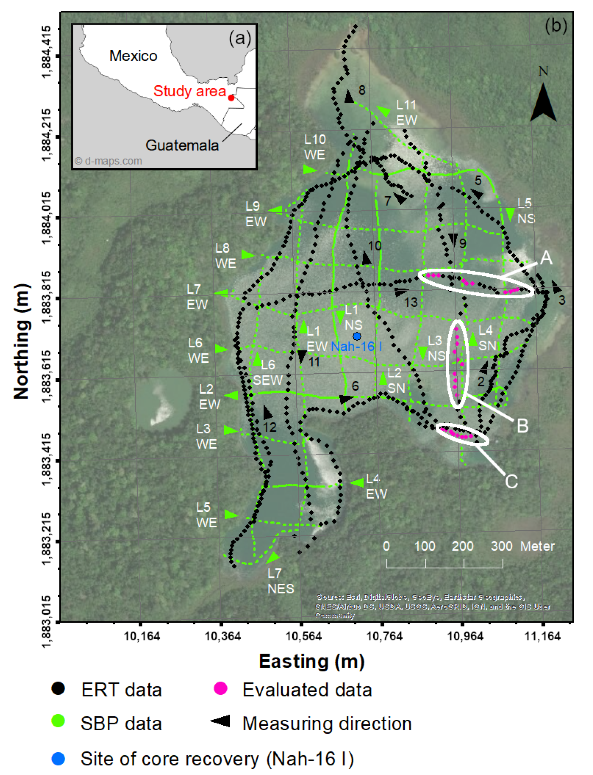
Abstract
:1. Introduction
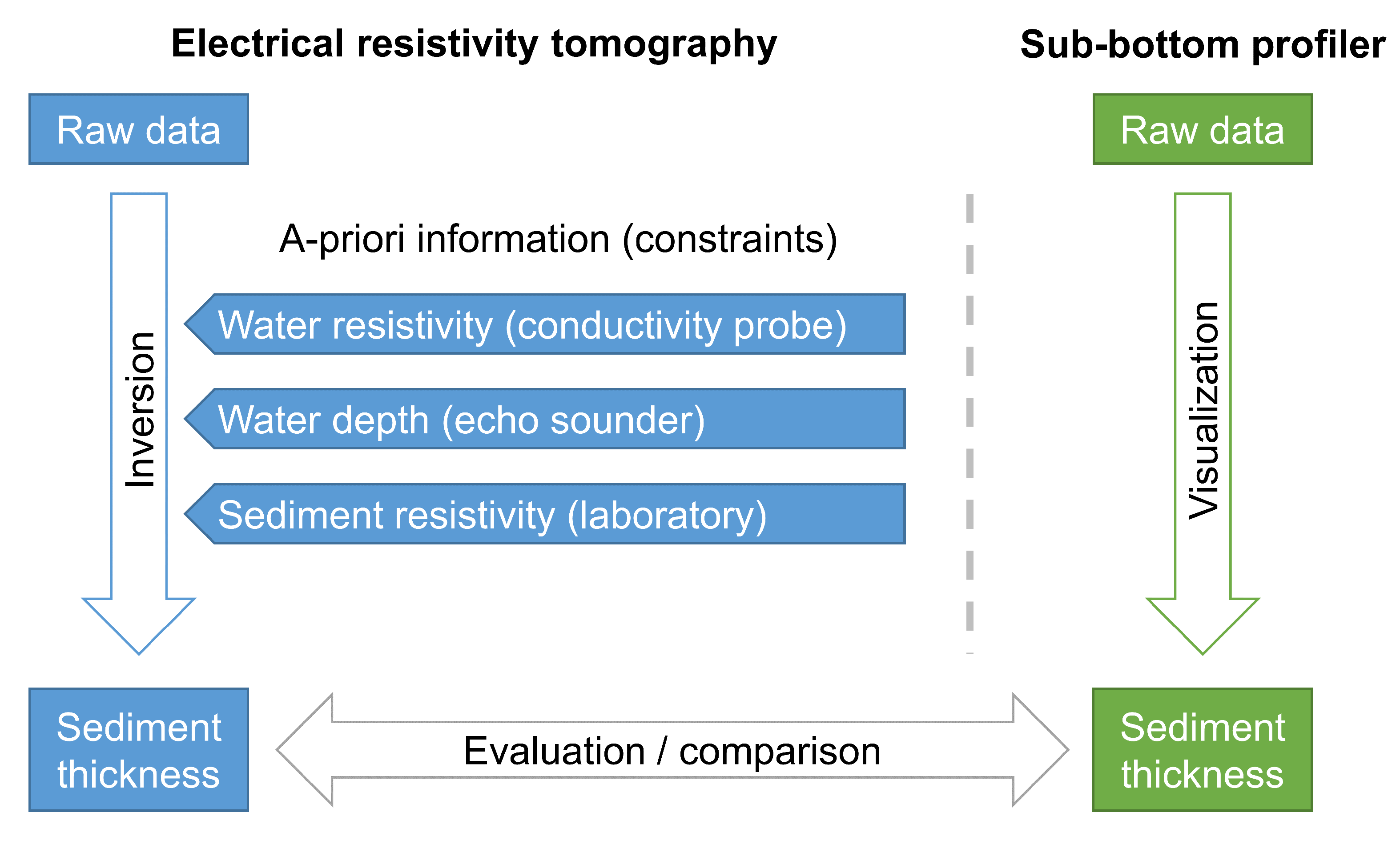
2. Materials and Methods
2.1. Study Site and Survey Layout
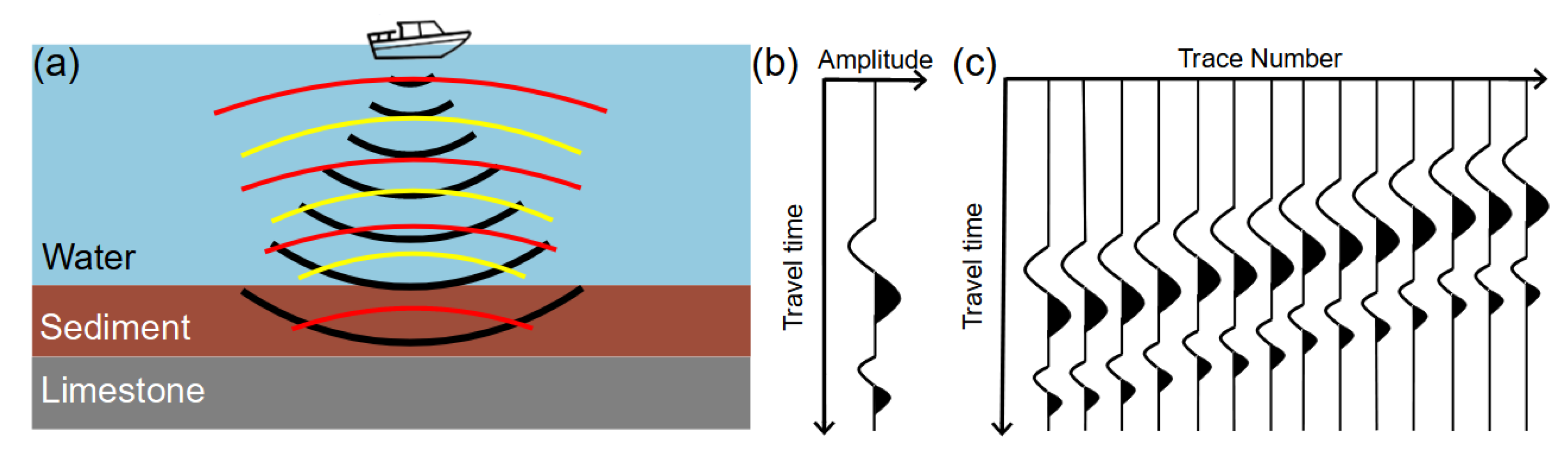
2.2. Sub-Bottom Profiler (SBP)
SBP Data Acquisition
2.3. Electrical-Resistivity Tomography (ERT)
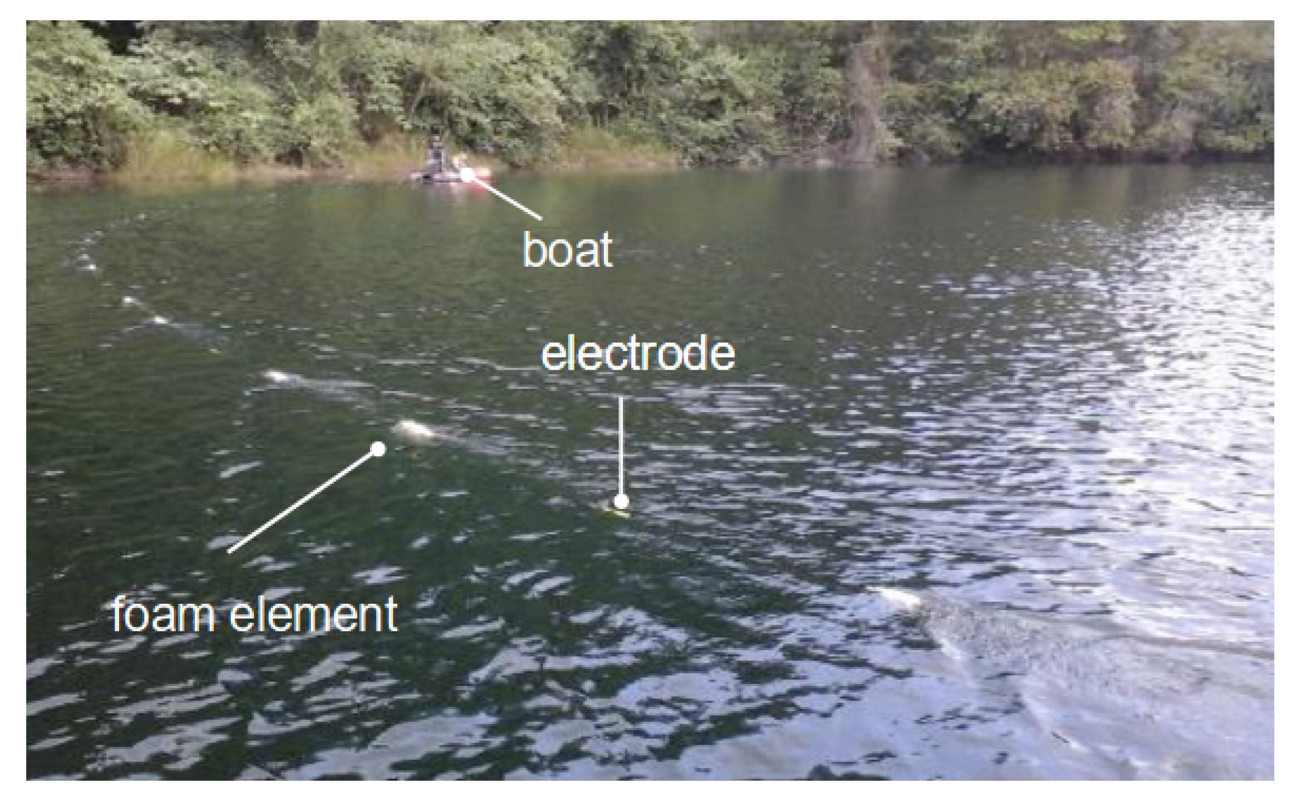
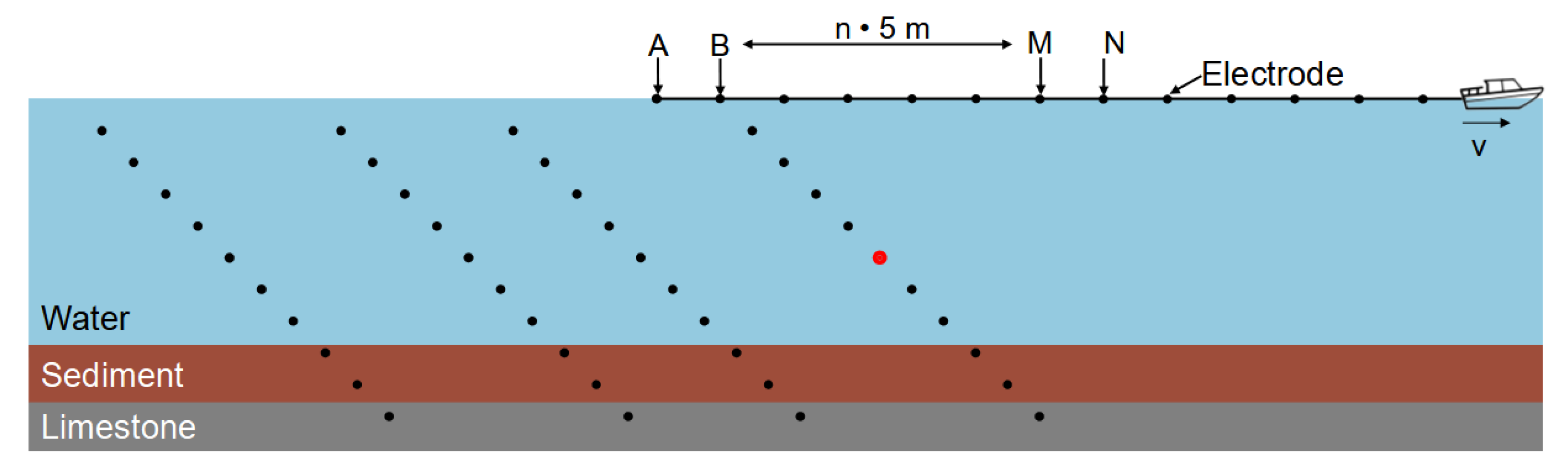
2.3.1. ERT Data Acquisition
2.3.2. Processing and Inversion of ERT Data
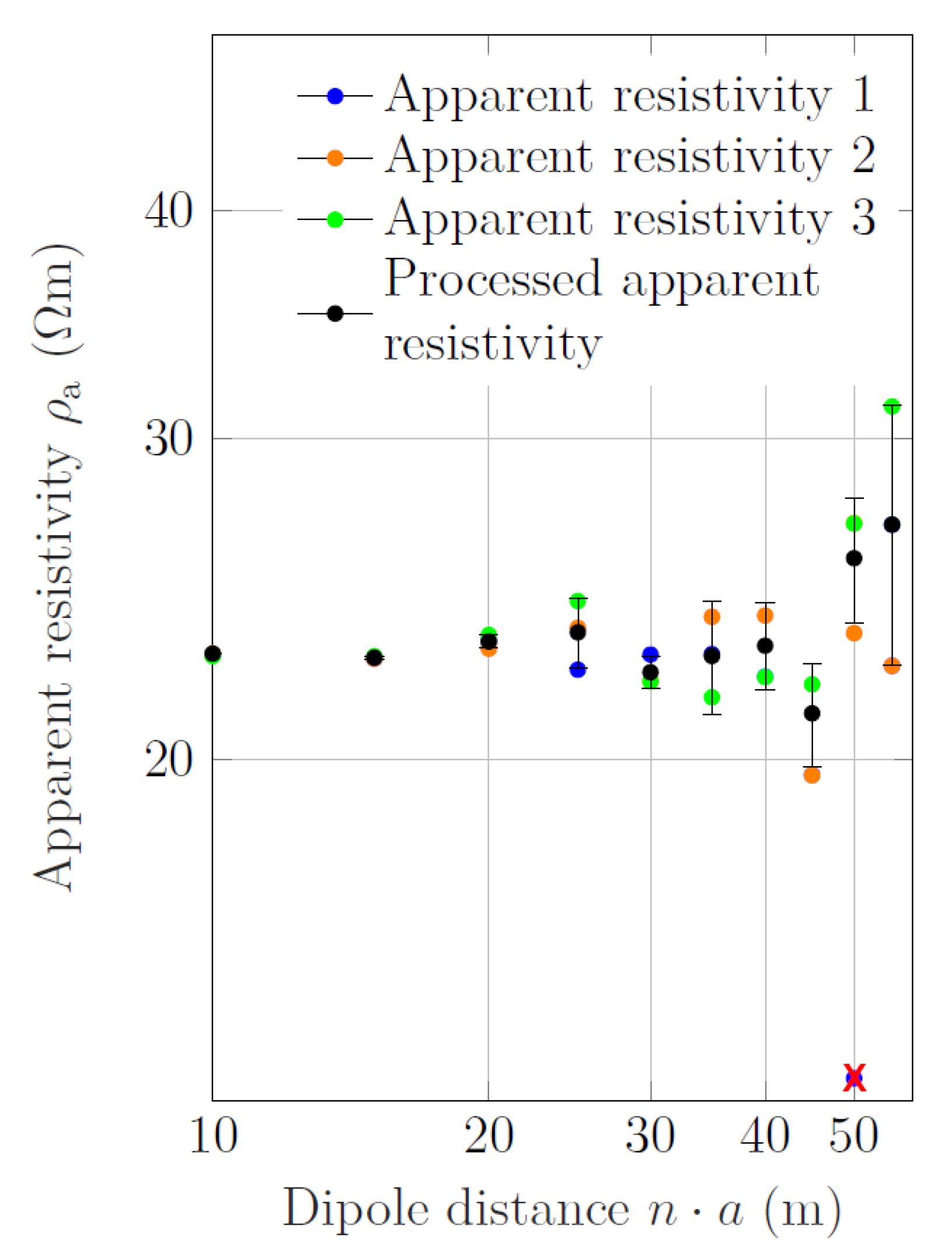
- The 10 apparent resistivity measurements at one single current–dipole location.
- The mean values of the 10 apparent resistivity measurements of x consecutive current–dipole locations (as sketched in Figure 5 for ).
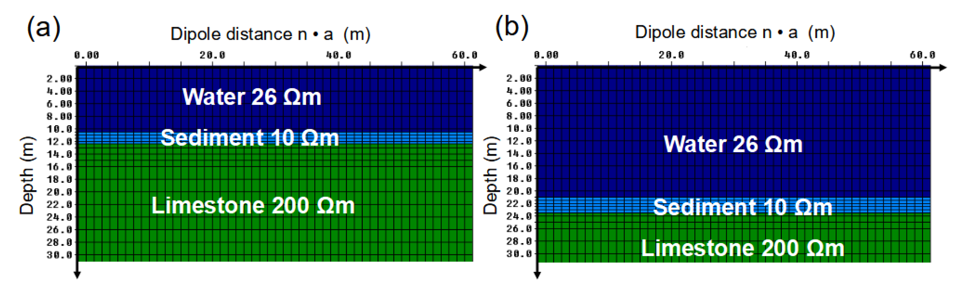
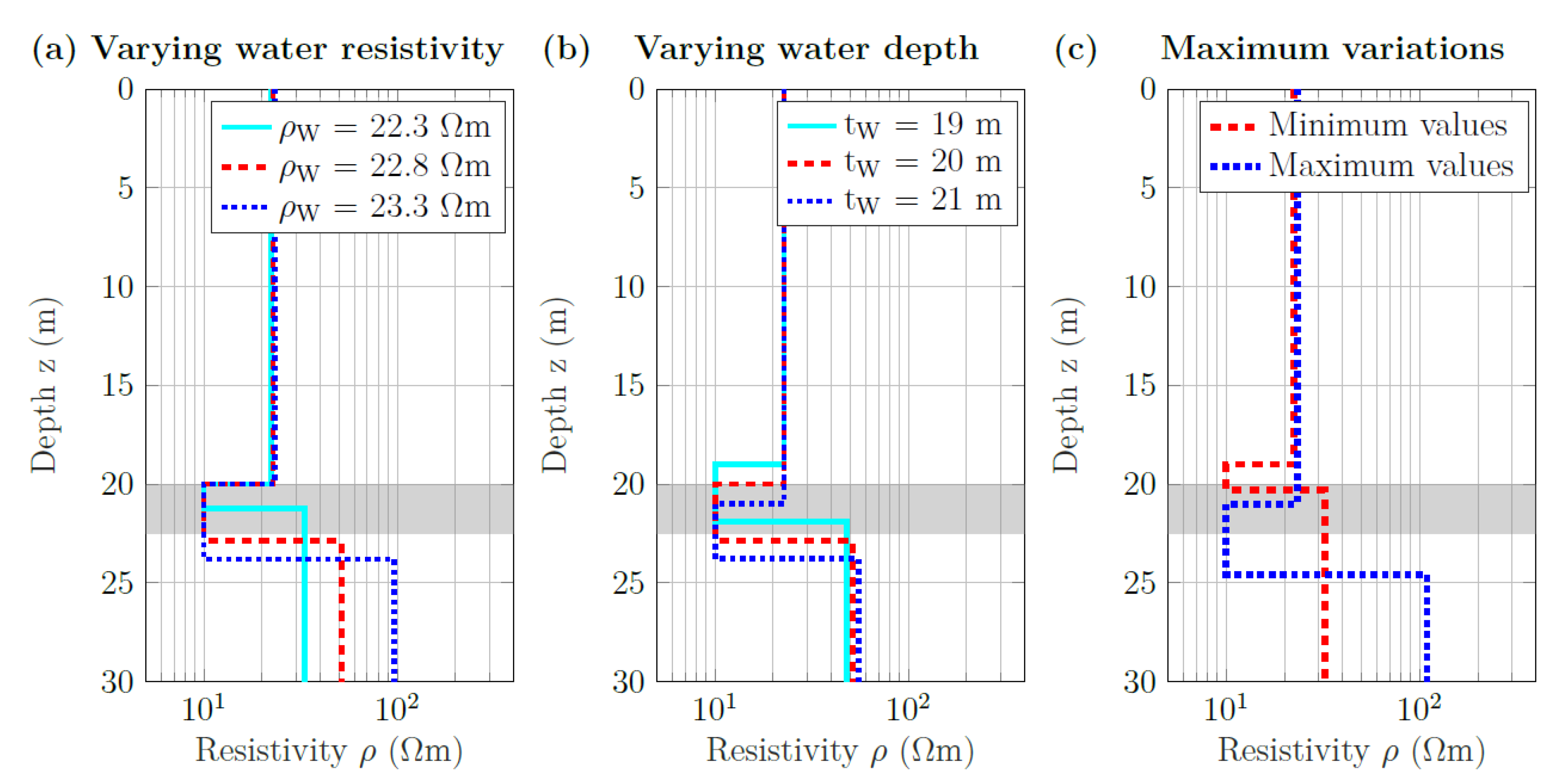
2.3.3. Forward Modeling Study
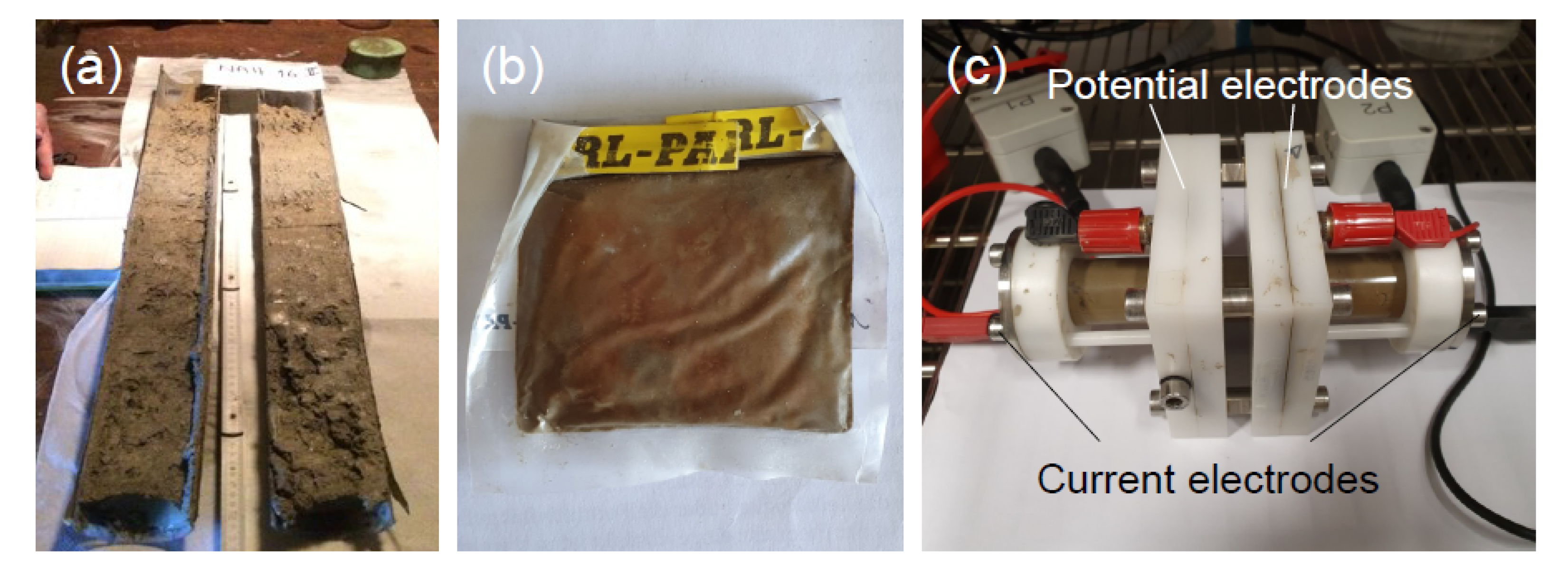
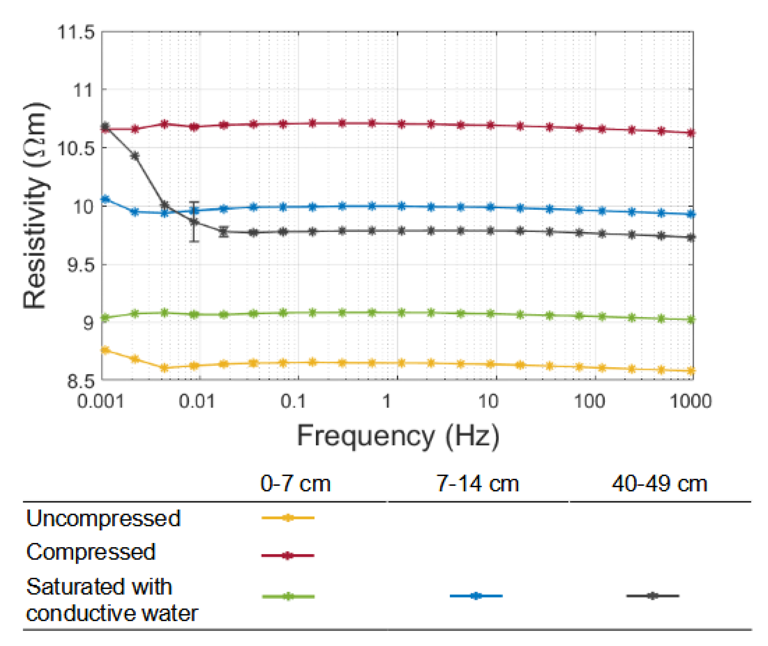
2.4. Laboratory Measurement of Sediment Resistivity
3. Results and Discussion
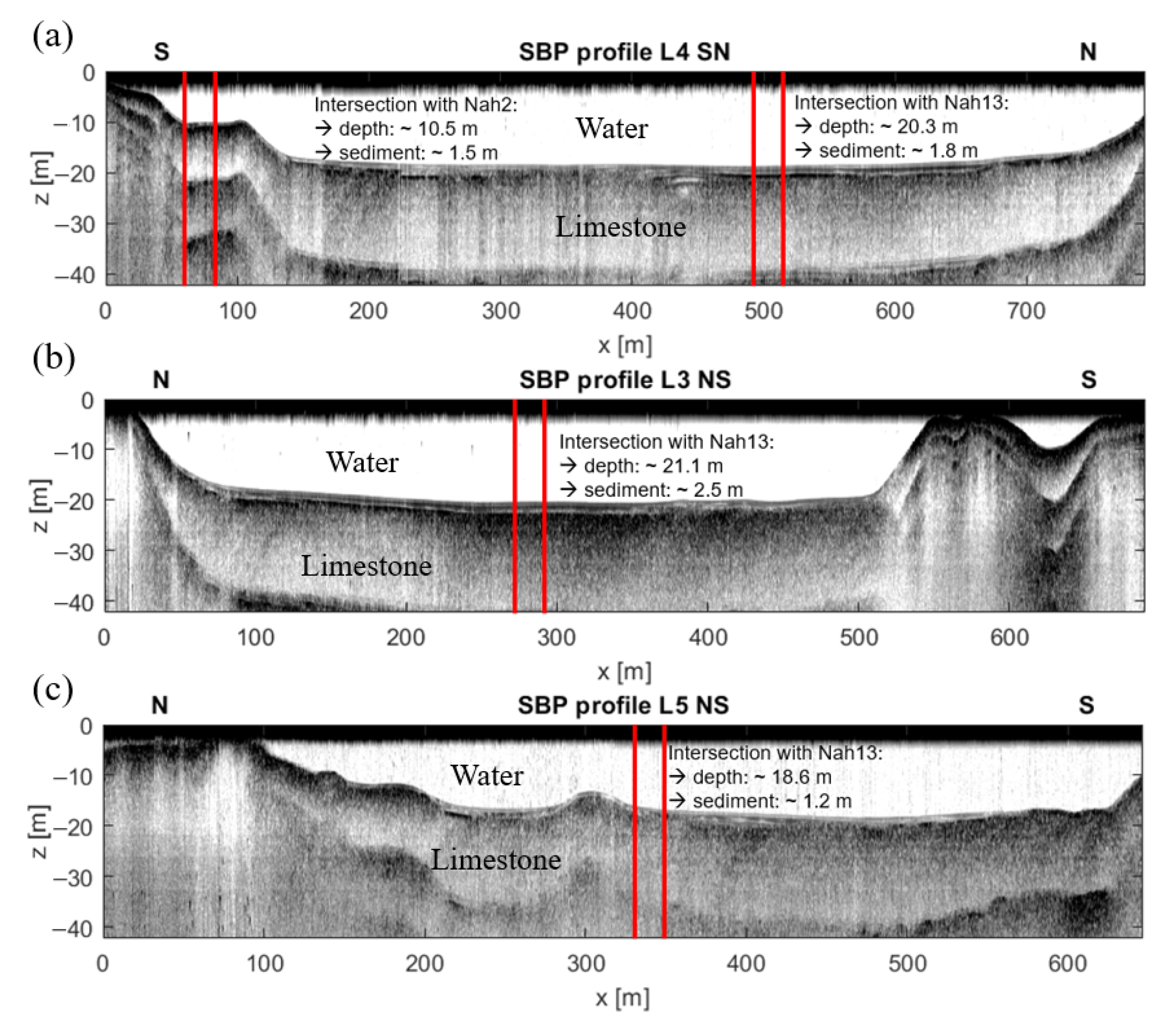
3.1. SBP Data Reveals Bathymetric Profile and Sediment Thickness
3.2. Laboratory Measurements Narrow down Sediment Resistivity
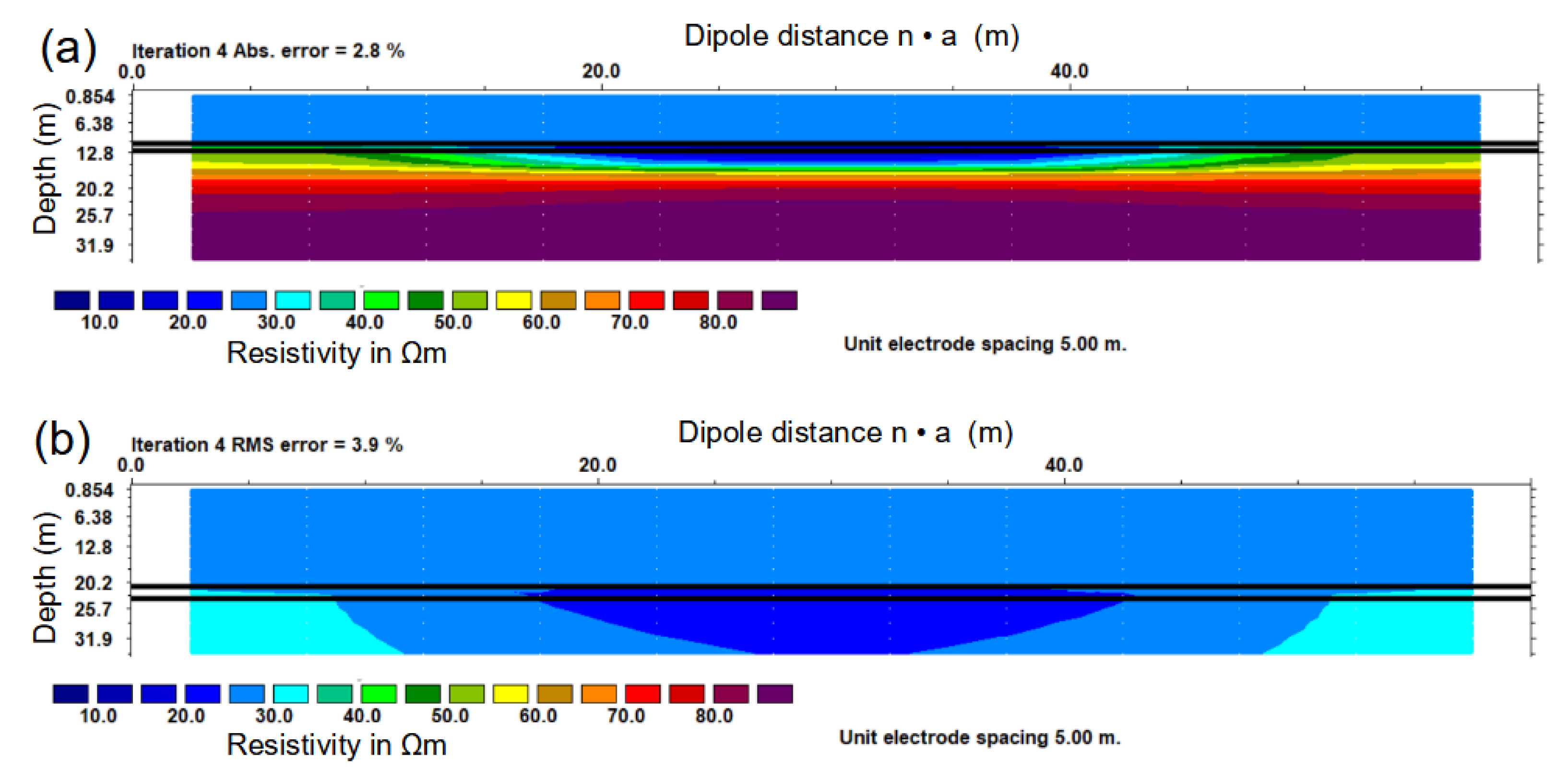
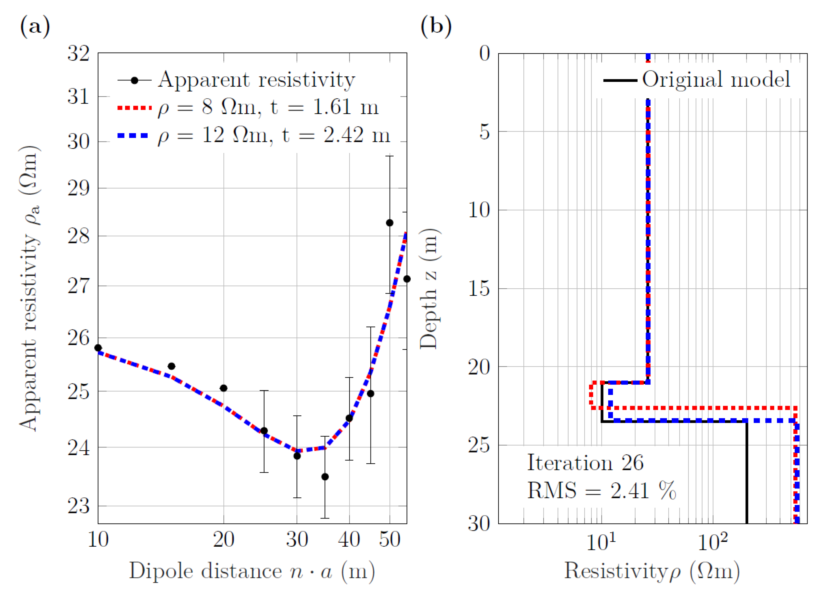
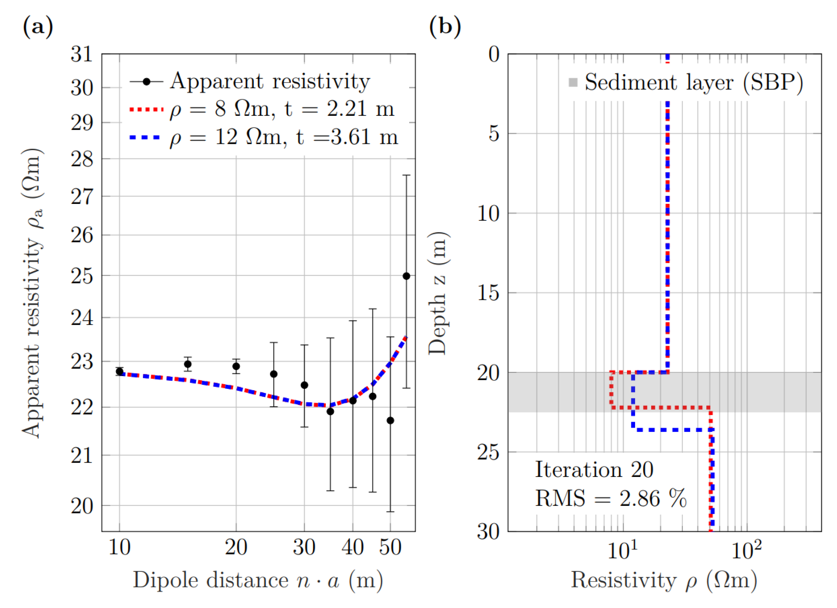
3.3. Modeling Study Shows That Constrained 1D Inversion Improves Sediment-Thickness Estimate from ERT Data
3.4. Constrained 1D Inversion Yields Sediment-Thickness Estimates Comparable to SBP Results
3.4.1. Performance in Deep Water
3.4.2. Performance in Shallow Water
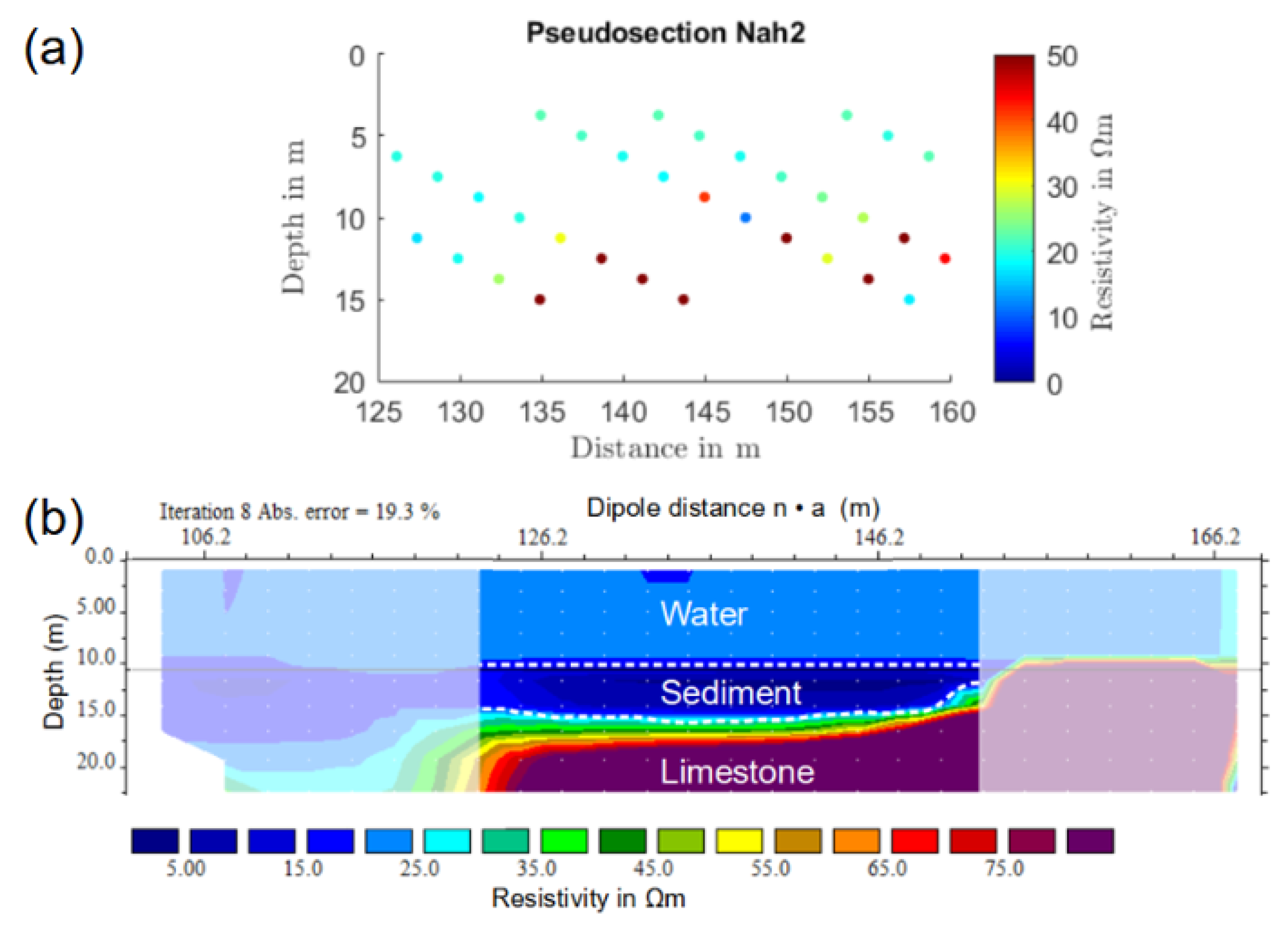
3.5. 2D Inversion of Shallow-Water ERT Data Were Not Able to Estimate Sediment Thickness
3.6. Assessment of the Approach
4. Conclusions
Author Contributions
Funding
Institutional Review Board Statement
Informed Consent Statement
Data Availability Statement
Acknowledgments
Conflicts of Interest
References
- Schindler, D. Lakes as Sentinels and Integrators for the Effects of Climate Change on Watersheds, Airsheds, and Landscapes. Limnol. Oceanogr. 2009, 54, 2349–2358. [Google Scholar] [CrossRef]
- Cohen, A. Paleolimnology: The History and Evolution of Lake Systems; Oxford University Press: Oxford, UK, 2003. [Google Scholar]
- Bradley, R. Lake Sediments. In Paleoclimatology: Reconstructing Climates of the Quaternary; Academic Press: Cambridge, MA, USA, 2015; pp. 319–343. [Google Scholar] [CrossRef]
- Moguel, B.; Pérez, L.; Alcaraz, L.; Blaz, J.; Caballero, M.; Muñoz-Velasco, I.; Becerra, A.; Laclette, J.; Ortega, B.; Romero-Oliva, C.; et al. Holocene life and microbiome profiling in ancient tropical Lake Chalco, Mexico. Sci. Rep. 2021, 11, 13848. [Google Scholar] [CrossRef] [PubMed]
- Chávez-Lara, C.; Roy, P.D.; Pérez, L.; Sankar, G.M.; Neri, V. Ostracode and C/N based paleoecological record from Santiaguillo Basin of subtropical Mexico over last 27 cal kyr BP. Rev. Mex. Cienc. Geológicas 2015, 32, 1. [Google Scholar]
- Vázquez-Molina, Y.; Correa-Metrio, A.; Zawisza, E.; Franco-Gaviria, F.; Pérez, L.; Romero, F.; Prado, B.; Charqueño-Célis, F.; Esperón-Rodríguez, M. Decoupled lake history and regional moisture availability in the middle elevations of tropical Mexico. Rev. Mex. Cienc. Geológicas 2016, 33, 355–364. [Google Scholar]
- Cohuo, S.; Macario-González, L.; Pérez, L.; Sylvestre, F.; Paillès, C.; Curtis, J.H.; Kutterolf, S.; Wojewódka, M.; Zawisza, E.; Szeroczyńska, K.; et al. Climate ultrastructure and aquatic community response to Heinrich Stadials (HS5a-HS1) in the continental northern Neotropics. Quat. Sci. Rev. 2018, 197, 75–91. [Google Scholar] [CrossRef]
- Cohuo, S.; Macario-González, L.; Wagner, S.; Naumann, K.; Echeverria-Galindo, P.; Pérez, L.; Curtis, J.; Brenner, M.; Schwalb, A. Influence of late Quaternary climate on the biogeography of Neotropical aquatic species as reflected by non-marine ostracodes. Biogeosciences 2020, 17, 145–161. [Google Scholar] [CrossRef] [Green Version]
- Obrist-Farner, J.; Brenner, M.; Curtis, J.; Kenney, W.; Salvinelli, C. Recent onset of eutrophication in Lake Izabal, the largest water body in Guatemala. J. Paleolimnol. 2019, 62, 1–14. [Google Scholar] [CrossRef]
- Hernandez, E.; Obrist-Farner, J.; Brenner, M.; Kenney, W.; Curtis, J.; Duarte, E. Natural and anthropogenic sources of lead, zinc, and nickel in sediments of Lake Izabal, Guatemala. J. Environ. Sci. 2020, 96, 117–126. [Google Scholar] [CrossRef]
- Lorenschat, J.; Pérez, L.; Correa-Metrio, A.; Brenner, M.; von Bramann, U.; Schwalb, A. Diversity and Spatial Distribution of Extant Freshwater Ostracodes (Crustacea) in Ancient Lake Ohrid (Macedonia/Albania). Diversity 2014, 6, 524–550. [Google Scholar] [CrossRef] [Green Version]
- Lozano, S.; Brown, E.; Ortega, B.; Caballero, M.; Werne, J.; Fawcett, P.; Schwalb, A.; Valero-Garcés, B.; Schnurrenberger, D.; O’Grady, R.; et al. Perforación profunda en el lago de Chalco: Reporte técnico. Bol. Soc. Geol. Mex. 2017, 69, 299–311. [Google Scholar] [CrossRef]
- Brown, E.T.; Caballero, M.; Cabral Cano, E.; Fawcett, P.J.; Lozano-García, S.; Ortega, B.; Pérez, L.; Schwalb, A.; Smith, V.; Steinman, B.A.; et al. Scientific drilling of Lake Chalco, Basin of Mexico (MexiDrill). Sci. Drill. 2019, 26, 1–15. [Google Scholar] [CrossRef] [Green Version]
- Chen, C.; McGee, D.; Woods, A.; Pérez, L.; Hatfield, R.; Edwards, R.; Cheng, H.; Valero-Garcés, B.; Lehmann, S.; Stoner, J.; et al. U-Th dating of lake sediments: Lessons from the 700 ka sediment record of Lake Junín, Peru. Quat. Sci. Rev. 2020, 244, 106422. [Google Scholar] [CrossRef]
- Pérez, L.; Correa-Metrio, A.; Cohuo, S.; González, L.M.; Echeverría-Galindo, P.; Brenner, M.; Curtis, J.; Kutterolf, S.; Stockhecke, M.; Schenk, F.; et al. Ecological turnover in neotropical freshwater and terrestrial communities during episodes of abrupt climate change. Quat. Res. 2021, 101, 26–36. [Google Scholar] [CrossRef]
- Bücker, M.; Lozano, S.; Ortega, B.; Caballero, M.; Pérez, L.; Caballero, L.; Carlos, P.; Sánchez-Galindo, A.; Villegas, F.; Flores Orozco, A.; et al. Geoelectrical and Electromagnetic Methods Applied to Paleolimnological Studies: Two Examples from Desiccated Lakes in the Basin of Mexico. Bol. Soc. Geol. Mex. 2017, 69, 279–298. [Google Scholar] [CrossRef]
- Bücker, M.; Flores Orozco, A.; Gallistl, J.; Steiner, M.; Aigner, L.; Hoppenbrock, J.; Glebe, R.; Morales Barrera, W.; Pita de la Paz, C.; García García, C.E.; et al. Integrated land and water-borne geophysical surveys shed light on the sudden drying of large karst lakes in southern Mexico. Solid Earth 2021, 12, 439–461. [Google Scholar] [CrossRef]
- Scholz, C.A. Applications of Seismic Sequence Stratigraphy in Lacustrine Basins. In Tracking Environmental Change Using Lake Sediments: Basin Analysis, Coring, and Chronological Techniques; Last, W.M., Smol, J.P., Eds.; Springer: Dordrecht, The Netherlands, 2001; pp. 7–22. [Google Scholar] [CrossRef]
- Bartole, R.; Lodolo, E.; Obrist-Farner, J.; Morelli, D. Sedimentary architecture, structural setting, and Late Cenozoic depocentre migration of an asymmetric transtensional basin: Lake Izabal, eastern Guatemala. Tectonophysics 2019, 750, 419–433. [Google Scholar] [CrossRef]
- Orlando, L. Some considerations on electrical resistivity imaging for characterization of waterbed sediments. J. Appl. Geophys. 2013, 95, 77–89. [Google Scholar] [CrossRef] [Green Version]
- Binley, A.; Kemna, A. DC Resistivity and Induced Polarization Methods. In Hydrogeophysics; Rubin, Y., Hubbard, S.S., Eds.; Springer: Dordrecht, The Netherlands, 2005; pp. 129–156. [Google Scholar] [CrossRef]
- Day-Lewis, F.D.; White, E.A.; Johnson, C.D., Jr.; Lane, J.W.L.; Belaval, M. Continuous resistivity profiling to delineate submarine groundwater discharge—Examples and limitations. Lead. Edge 2006, 25, 724–728. [Google Scholar] [CrossRef]
- Kwon, H.S.; Kim, J.H.; Ahn, H.Y.; Yoon, J.S.; Kim, K.S.; Jung, C.K.; Lee, S.B.; Uchida, T. Delineation of a Fault Zone Beneath a Riverbed By an Electrical Resistivity Survey Using a Floating Streamer Cable. Explor. Geophys. 2005, 36, 50–58. [Google Scholar] [CrossRef]
- Befus, K.; Cardenas, M.; Ong, J.; Zlotnik, V. Classification and delineation of groundwater–lake interactions in the Nebraska Sand Hills (USA) using electrical resistivity patterns. Hydrogeol. J. 2012, 20. [Google Scholar] [CrossRef]
- McLachlan, P.; Chambers, J.; Uhlemann, S.; Sorensen, J.; Binley, A. Electrical resistivity monitoring of river-groundwater interactions in a Chalk river and neighbouring riparian zone. Near Surf. Geophys. 2020, 18, 385–398. [Google Scholar] [CrossRef]
- Colombero, C.; Comina, C.; Gianotti, F.; Sambuelli, L. Waterborne and on-land electrical surveys to suggest the geological evolution of a glacial lake in NW Italy. J. Appl. Geophys. 2014, 105, 191–202. [Google Scholar] [CrossRef] [Green Version]
- McLachlan, P.; Chambers, J.; Uhlemann, S.; Binley, A. Limitations and considerations for electrical resistivity and induced polarization imaging of riverbed sediments: Observations from laboratory, field, and synthetic experiments. J. Appl. Geophys. 2020, 183, 104173. [Google Scholar] [CrossRef]
- Dahlin, T.; Loke, M. Underwater ERT surveying in water with resistivity layering with example of application to site investigation for a rock tunnel in central Stockholm. Near Surf. Geophys. 2018, 16, 230–237. [Google Scholar] [CrossRef] [Green Version]
- Vozoff, K.; Jupp, D.L.B. Joint Inversion of Geophysical Data. Geophys. J. Int. 1975, 42, 977–991. [Google Scholar] [CrossRef] [Green Version]
- Hermans, T.; Vandenbohede, A.; Lebbe, L.; Martin, R.; Kemna, A.; Beaujean, J.; Nguyen, F. Imaging artificial salt water infiltration using electrical resistivity tomography constrained by geostatistical data. J. Hydrol. 2012, 438–439, 168–180. [Google Scholar] [CrossRef] [Green Version]
- Doetsch, J.; Linde, N.; Pessognelli, M.; Green, A.; Günther, T. Constraining 3-D electrical resistance tomography with GPR reflection data for improved aquifer characterization. J. Appl. Geophys. 2012, 78, 68–76. [Google Scholar] [CrossRef]
- Loke, M.H.; Barker, R.D. Least-squares deconvolution of apparent resistivity pseudosections. Geophysics 1995, 60, 1682–1690. [Google Scholar] [CrossRef]
- Ekinci, Y.L.; Demirci, A. A Damped Least-Squares Inversion Program for the Interpretation of Schlumberger Sounding Curves. J. Appl. Sci. 2008, 8. [Google Scholar] [CrossRef] [Green Version]
- Mandujano, J.; Keppie, J. Middle Miocene Chiapas fold and thrust belt of Mexico: A result of collision of the Tehuantepec Transform/Ridge with the Middle America Trench. Geol. Soc. London Spec. Publ. 2009, 327, 55–69. [Google Scholar] [CrossRef]
- García-Gil, J.; Lugo Hupb, J. Las formas del relieve y los tipos de vegetación en la Selva Lacandona. In Reserva de la Biósfera Montes Azules, Selva Lacandona: Investigación para su Conservación; Sánchez, M.A.V., Olmos, M.A.R., Eds.; Publicaciones Especiales Ecosfera: Dordrecht, The Netherlands, 1992; pp. 39–49. [Google Scholar]
- Rubio Sandoval, C.Z. Estudio Paleoambiental en dos Lagos káRsticos de la Selva Lacandona, Chiapas, Mexico, Durante los últimos 500 años Utilizando Indicadores Biológicos y geoquíMicos. Master’s Thesis, Universidad Nacional Autónoma de México, Mexico City, Mexico, 2019. [Google Scholar]
- Díaz, K.; Pérez, L.; Correa-Metrio, A.; Franco-Gaviria, F.; Echeverría-Galindo, P.; Curtis, J.; Brenner, M. Holocene environmental history of tropical, mid-altitude Lake Ocotalito, México, inferred from ostracodes and non-biological indicators. Holocene 2017, 27, 095968361668738. [Google Scholar] [CrossRef]
- Echeverría Galindo, P.G.; Pérez, L.; Correa-Metrio, A.; Avendano, C.E.; Moguel, B.; Brenner, M.; Cohuo, S.; Macario, L.; Caballero, M.; Schwalb, A. Tropical freshwater ostracodes as environmental indicators across an altitude gradient in Guatemala and Mexico. Rev. Biol. Trop. 2019, 67, 1037–1058. [Google Scholar] [CrossRef]
- Charqueño, N.; Garibay, M.; Sigala, I.; Brenner, M.; Echeverría-Galindo, P.; Lozano, S.; Massaferro, J.; Pérez, L. Testate amoebae (Amoebozoa: Arcellinidae) as indicators of dissolved oxygen concentration and water depth in lakes of the Lacandón Forest, southern Mexico. J. Limnol. 2020, 79. [Google Scholar] [CrossRef]
- Dondurur, D. Acquisition and Processing of Marine Seismic Data; Elsevier: Amsterdam, The Netherlands, 2018; p. 606. [Google Scholar] [CrossRef]
- Bashkardin, V. GSEGYView (Version 0.2). 2013. Available online: https://sourceforge.net/projects/gsegyview/ (accessed on 26 November 2021).
- Flores Orozco, A.; Bücker, M.; Steiner, M.; Malet, J.P. Complex-conductivity imaging for the understanding of landslide architecture. Eng. Geol. 2018, 243, 241–252. [Google Scholar] [CrossRef]
- Knödel, K.; Krummel, H.; Lange, G. Handbuch zur Erkundung des Untergrundes von Deponien und Altlasten/BGR, Bundesanstalt für Geowissenschaften und RohstoffeBd. 3: Geophysik, 2. überarbeitete auflage ed.; Springer: Berlin/Heidelberg, Germany, 2005. [Google Scholar]
- Nyman, D.C.; Landisman, M. VES dipole-dipole filter coefficients. Geophysics 1977, 42, 1037–1044. [Google Scholar] [CrossRef]
- Hoppenbrock, J.; Bücker, M.; Gallistl, J.; Flores Orozco, A.; Pita de la Paz, C.; García García, C.E.; Razo Pérez, J.A.; Buckel, J.; Pérez, L. Data set, Evaluation of Lake Sediment Thickness from Water-Borne Electrical Resistivity Tomography Data (v1.0). Zenodo 2021. [Google Scholar] [CrossRef]
- Loke, M. RES2DMOD ver. 3.03.06: Rapid 2D Resistivity and I.P. forward Modeling Using the Finite-Difference and Finite-Element Methods. 2016. Available online: https://www.geotomosoft.com/downloads.php (accessed on 26 November 2021).
- Bairlein, K.; Hördt, A.; Nordsiek, S. The influence on sample preparation on spectral induced polarization of unconsolidated sediments. Near Surf. Geophys. 2014, 12, 667–678. [Google Scholar] [CrossRef]
- Przyklenk, A.; Hördt, A.; Radic, T. Capacitively-Coupled Resistivity measurements to determine frequency dependent electrical parameters in periglacial environment—Theoretical considerations and first field tests. Geophys. J. Int. 2016, 206, ggw178. [Google Scholar] [CrossRef] [Green Version]
- Lowrie, W. Seismology and the internal structure of the Earth. In Fundamentals of Geophysics, 2nd ed.; Cambridge University Press: Cambridge, UK, 2007; pp. 121–206. [Google Scholar] [CrossRef]
- Telford, W.M.; Geldart, L.P.; Sheriff, R.E. Resistivity Methods. In Applied Geophysics, 2nd ed.; Cambridge University Press: Cambridge, UK, 1990; pp. 522–577. [Google Scholar] [CrossRef]
- Rücker, C.; Günther, T.; Wagner, F.M. pyGIMLi: An open-source library for modelling and inversion in geophysics. Comput. Geosci. 2017, 109, 106–123. [Google Scholar] [CrossRef]
- Lachhab, A.; Booterbaugh, A.; Beren, M. Bathymetry and Sediment Accumulation of Walker Lake, PA Using Two GPR Antennas in a New Integrated Method. J. Environ. Eng. Geophys. 2015, 20, 245–255. [Google Scholar] [CrossRef] [Green Version]
- Boehrer, B.; Schultze, M. Stratification of lakes. Rev. Geophys. 2008, 46. [Google Scholar] [CrossRef] [Green Version]
- Pérez, L.; Bugja, R.; Lorenschat, J.; Brenner, M.; Curtis, J.; Hoelzmann, P.; Islebe, G.; Scharf, B.; Schwalb, A. Aquatic ecosystems of the Yucatán Peninsula (Mexico), Belize, and Guatemala. Hydrobiologia 2011, 661, 407–433. [Google Scholar] [CrossRef]
- Baumgartner, F. A new method for geoelectrical investigations underwater1. Geophys. Prospect. 1996, 44, 71–98. [Google Scholar] [CrossRef]


Publisher’s Note: MDPI stays neutral with regard to jurisdictional claims in published maps and institutional affiliations. |
© 2021 by the authors. Licensee MDPI, Basel, Switzerland. This article is an open access article distributed under the terms and conditions of the Creative Commons Attribution (CC BY) license (https://creativecommons.org/licenses/by/4.0/).
Share and Cite
Hoppenbrock, J.; Bücker, M.; Gallistl, J.; Flores Orozco, A.; de la Paz, C.P.; García García, C.E.; Razo Pérez, J.A.; Buckel, J.; Pérez, L. Evaluation of Lake Sediment Thickness from Water-Borne Electrical Resistivity Tomography Data. Sensors 2021, 21, 8053. https://doi.org/10.3390/s21238053
Hoppenbrock J, Bücker M, Gallistl J, Flores Orozco A, de la Paz CP, García García CE, Razo Pérez JA, Buckel J, Pérez L. Evaluation of Lake Sediment Thickness from Water-Borne Electrical Resistivity Tomography Data. Sensors. 2021; 21(23):8053. https://doi.org/10.3390/s21238053
Chicago/Turabian StyleHoppenbrock, Johannes, Matthias Bücker, Jakob Gallistl, Adrián Flores Orozco, Carlos Pita de la Paz, César Emilio García García, José Alberto Razo Pérez, Johannes Buckel, and Liseth Pérez. 2021. "Evaluation of Lake Sediment Thickness from Water-Borne Electrical Resistivity Tomography Data" Sensors 21, no. 23: 8053. https://doi.org/10.3390/s21238053