
Complex Pearson Correlation Coefficient for EEG Connectivity Analysis


1
Faculty of Engineering, Department of Automation and Electronics, University of Rijeka, 51000 Rijeka, Croatia
2
Faculty of Mathematics, Natural Sciences and Information Technologies, University of Primorska, 6000 Koper, Slovenia
*
Author to whom correspondence should be addressed.
Sensors 2022, 22(4), 1477; https://doi.org/10.3390/s22041477
Submission received: 21 January 2022
/
Revised: 9 February 2022
/
Accepted: 11 February 2022
/
Published: 14 February 2022
(This article belongs to the Special Issue EEG Signal Processing for Biomedical Applications)
Abstract
:In the background of all human thinking—acting and reacting are sets of connections between different neurons or groups of neurons. We studied and evaluated these connections using electroencephalography (EEG) brain signals. In this paper, we propose the use of the complex Pearson correlation coefficient (CPCC), which provides information on connectivity with and without consideration of the volume conduction effect. Although the Pearson correlation coefficient is a widely accepted measure of the statistical relationships between random variables and the relationships between signals, it is not being used for EEG data analysis. Its meaning for EEG is not straightforward and rarely well understood. In this work, we compare it to the most commonly used undirected connectivity analysis methods, which are phase locking value (PLV) and weighted phase lag index (wPLI). First, the relationship between the measures is shown analytically. Then, it is illustrated by a practical comparison using synthetic and real EEG data. The relationships between the observed connectivity measures are described in terms of the correlation values between them, which are, for the absolute values of CPCC and PLV, not lower that 0.97, and for the imaginary component of CPCC and wPLI—not lower than 0.92, for all observed frequency bands. Results show that the CPCC includes information of both other measures balanced in a single complex-numbered index.
1. Introduction
A human brain contains on average about 100 billion () neurons connected by about 100 trillion () synapses. The neurons are anatomically organized in different spatial regions and functionally interact over different time points [1]. In this work, electroencephalography (EEG) was used to record neuron activity. EEG is an electrophysiological monitoring method for observing neurophysiological changes related to postsynaptic activity in the neocortex, i.e., a method for recording the electrical activity of the brain [2]. Monitoring brain activity using this method provides high temporal resolution. This property makes EEG one of the most suitable monitoring methods for non-invasive detection of neurons’ interactions inside the brain and, consequently, for detection of information transmission within the same brain regions and between different brain regions [3]. Brain connectivity analysis is generally divided into two types: structural and functional. Tracking the direction of fibers between different brain regions or within a brain region is called structural connectivity analysis [4]. The most suitable recording methods for determining structural connectivity are magnetic resonance imaging (MRI) [5] and diffusion tensor imaging (DTI) [6]. On the other hand, functional connectivity analysis can be defined as an analysis of the amount of information transmitted between brain regions or within a brain region. This type of connectivity analysis is usually divided into two groups: undirected and directed. Undirected connectivity measures evaluate the degree of connectivity, while directed connectivity measures evaluate the degree and direction of connectivity between observed brain regions. In this paper, we focus on undirected connectivity measures. Different cognitive tasks require different information flows within a brain area or between different brain areas. This is due to the fact that neuronal oscillations are background mechanisms essential for dynamic cooperation in the brain [7,8,9,10,11,12].
The most suitable methods for monitoring brain activity to determine functional connectivity are magnetoencephalography (MEG) and electroencephalography (EEG) due to their good temporal resolutions [13].
Different types of measures can be used to determine functional connectivity, such as phase synchronization, generalized synchronization measures, linear temporal correlation, etc. [14,15,16]. In this paper, we focus on undirected phase synchronization measures. The most often used measures are the phase locking value (PLV) [17,18] and the weighted phase lag index (wPLI) [19]. The main difference between these two measures is the ability to avoid the effect of volume conduction.
The PLV index is based on phase differences of signals from two EEG channels. For a set of N time points, it calculates an average of N unit vectors that represent the phase difference between the signals of both channels. The PLV value of zero represents no connection between the observed signals’ regions and the maximum PLV value of one represents a perfect connection. Although very widely used, a drawback of the PLV measure is the tendency to be biased towards higher values due to volume conduction [17].
The phase lag index (PLI) was designed as a solution to avoid the misinterpretation of volume conduction as a connectivity component [17]. Volume conduction reflects in the appearance of signal components with phase differences closer to 0 or . PLI avoids them by only considering the number of samples with positive and negative phase differences. Only if the number of samples in one group, i.e., positive or negative, is predominant then PLI gets value close to one. This cancels out the components with phase angle distributions centered at 0 and .
The extended version of the PLI is the weighted phase lag index (wPLI [19]). The wPLI measure adds weighting of samples by the imaginary component of the cross-spectral density. Because the real component of cross spectral density is not considered, samples where the phase differences are close to 0 or have no contribution to the connectivity estimation and signal components that may arise due to volume conduction have no influence.
There are several other undirected connectivity measures, such as coherence, imaginary part of coherence, mutual information, etc., but for the purposes of this article, we limit our analysis to only those two most common ones, i.e., PLV and wPLI. They complement one another, providing connectivity estimation with and without consideration of the volume conduction effect. As an alternative, we propose a complex Pearson correlation coefficient (CPCC), which in a single unique measure provides information of both connectivity components.
The rest of the article is structured in the following way. In Section 2, we propose the complex Pearson correlation coefficient as a novel measure of undirected channel connectivity, review the PLV and wPLI measures, and analytically show their relationships to CPCC. In section three, the relationship is demonstrated with practical experiments, using synthetic and real EEG signals. We end the paper with a discussion and conclusion.
2. Methods
In this section, we define the proposed complex Pearson correlation measure (CPCC) and show its analytical relationship with PLV and wPLI connectivity measures.
2.1. Complex Pearson Correlation Coefficient as a Measure of Undirected Connectivity
Various types of complex correlation calculations are used in the literature [20], and in different research fields, such as geophysics [21], radar systems [22], optics [23], etc. In this section, we propose the use of complex Pearson correlation coefficient for EEG connectivity analysis.
Pearson’s linear correlation coefficient (r) is the most commonly used linear correlation coefficient. It is a statistical measure of the degree to which variables change their values in relation to each other, or in other words, expresses the level to which two variables are linearly related. It is defined as follows:
Here, N is the number of samples, and , are the series being analyzed, represents mean values of observed series, and is the complex conjugate operator (if the values in series are complex). The resulting r ranges from −1 (indicating perfect negative correlation) to +1 (indicating perfect positive correlation). A zero value is an indicator of no linear signal relationship. Assuming that EEG signals for the analysis should be pre-filtered, which removes DC signal components, the equation can be simplified:
The numerator in the Equation (2) can be understood as a time-averaged temporal estimation of sample relationship, while the denominator is a weighting factor to obtain the desired range from −1 to 1. Let us first focus to the numerator. For two oscillatory signals represented as series of real values, the temporal relationship estimation is also an oscillatory signal. Consequently, the temporal contribution of a single time step does not have any direct meaning and at least one period of signal samples need to be averaged to become informative. To improve temporal meaningfulness of the estimation, analytic signal representations can be used instead of real valued ones. Analytic signal sample is a complex number that adds an imaginary part indicating the oscillatory nature of the signal to its existent real valued part. Thus, in addition to a real signal value, the analytic signal sample includes the information of signal instantaneous amplitude and instantaneous phase, which can be represented as a vector in a complex plane. Because basic sinusoidal oscillatory signal keeps the instantaneous amplitude constant over time while its instantaneous phase increases linearly, these vectors are also called phasors. For two phase-locked signals the phase difference is constant and the numerator of Equation (2) gets constant over time, too. Its real value represents the dot product of the phasors, while its imaginary part equals the size of the cross product. Altogether the product of two phasors of two analytic signals is analogous to the cross spectral density for the stationary or quasi-stationary signals. The denominator of Equation (2), needed for scaling, relates to the power of both signals. The final result when using analytic signals is the complex Pearson correlation coefficient (CPCC):
where denotes analytic signals.
The analytic signal representation is defined only for narrow frequency band signals. In such cases analytic signals can be computed from real ones by adding imaginary part equal to the Hilbert transform (HT) of the original signal:
where HT (x(t)) represents the Hilbert transform of x (real signal) and is an analytic signal, as explained in [17]. With HT we obtain a phasor influenced by all the frequencies in the observed narrow band. Phasors can also be obtained using the discrete Fourier transform, where one phasor presents each frequency component, but only stationary, without temporal dimension. HT provides this additional temporal perspective, which enables analysis of non-stationary signals. Because EEG signals are non-stationary, in this paper we limit to the analysis of their narrow band pre-filtered components with the analytic form obtained using HT.
Connectivity measures estimate the relationship between two signals and this can be performed using the CPCC. The in-phase signals have high real CPCC part and zero imaginary part. On the other hand, imaginary component represents the relationship between signals with the phase lag of . Thus, the connectivity of two brain regions can be estimated considering both parts of the complex CPCC value for the corresponding EEG signals, by computing its absolute value (absCPCC). In such a case the obtained value should be related to the PLV value. When the volume conduction effect needs to be avoided, only the imaginary component shall be used (imCPCC). Such estimation is expected to be related to the wPLI value.
2.2. Phase Locking Value PLV and Its Relation to CPCC
Phase-locking value (PLV) is calculated based on the phase differences of the two analytical signals [17,18]:
In Equation (5), represents the phase difference and N represents the number of samples. The instantaneous phase difference is defined as:
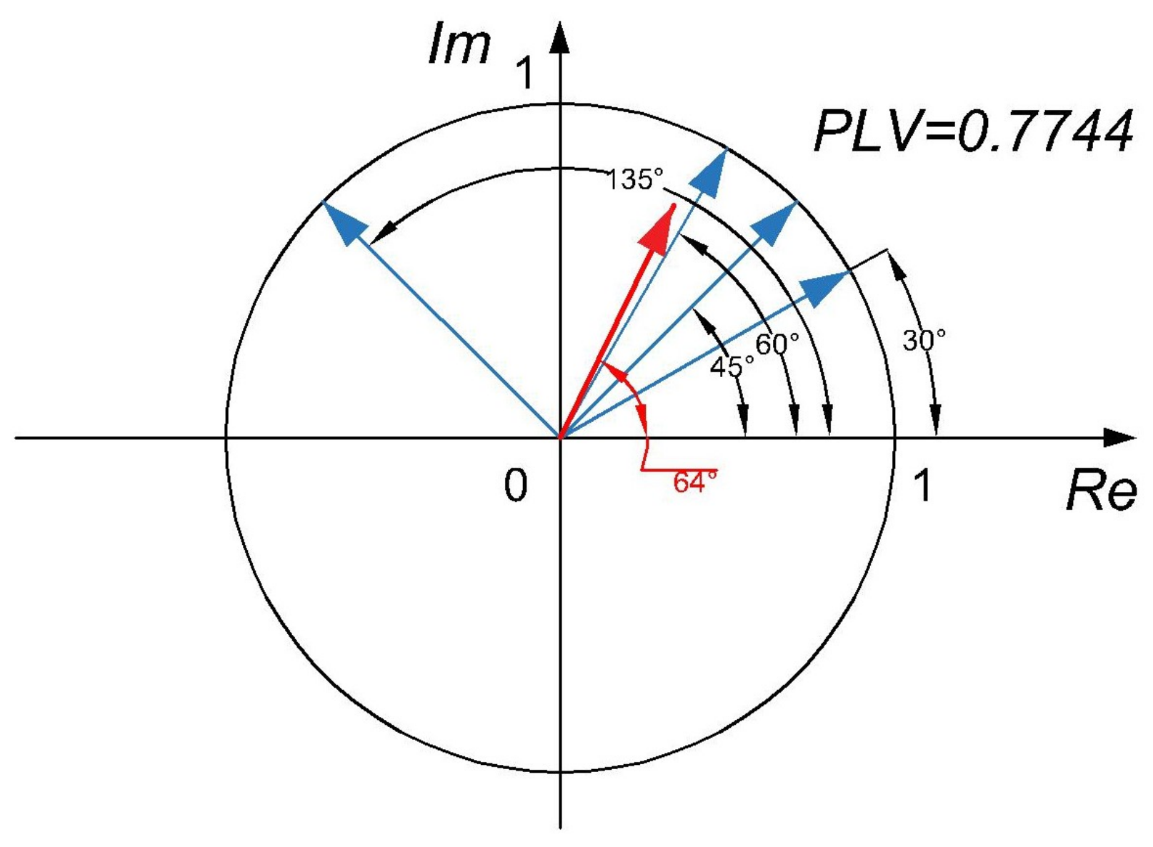
where and stand for the phase angles at n-th sample. In order to obtain instantaneous phases, analytical signals need to be computed, using (HT). Computation of PLV can be visualized by creating a set of N unit vectors corresponding to N time samples, see Figure 1. Phase angles of those vectors are equal to phase differences between the two EEG signals for samples from 1 to N. All the N unit vectors representing phase differences are averaged to obtain PLV.
The high value of PLV is obtained when the vectors are well clustered, which means that the phase difference between the two EEG channels is mostly constant for all the time samples On the other hand, when the phase difference between the two channels is changing with time, the unit vectors are scattered, which results in low PLV value.
The lack of this measure is its tendency to falsely over-estimate the connectivity level due to the volume conduction. The reason is that the volume conduction enables a signal from a single source to be measured on both EEG electrodes under consideration, which results in a zero-phase difference over a larger time interval, leading to a larger PLV value.
In order to prove our assumption that the absolute value of the complex Pearson correlation is related to the PLV index, the Equation (2) can be rewritten in the following way:
where represents the instantaneous amplitude of a complex signal.
2.3. Weighted Phase Lag Index wPLI and Its Relation to CPCC
The PLI and wPLI measures of connectivity address the volume conduction problem. Let us first present the PLI measure, as a transitional step towards a more refined weighted PLI measure (wPLI). The PLI is defined as [17]:
where N is the number of samples. In the original definition [24], is the cross-spectral density of the observed signals defined by Fourier transform. In [17], PLI was defined using analytical signals obtained by HT and the cross-spectral density is defined as:
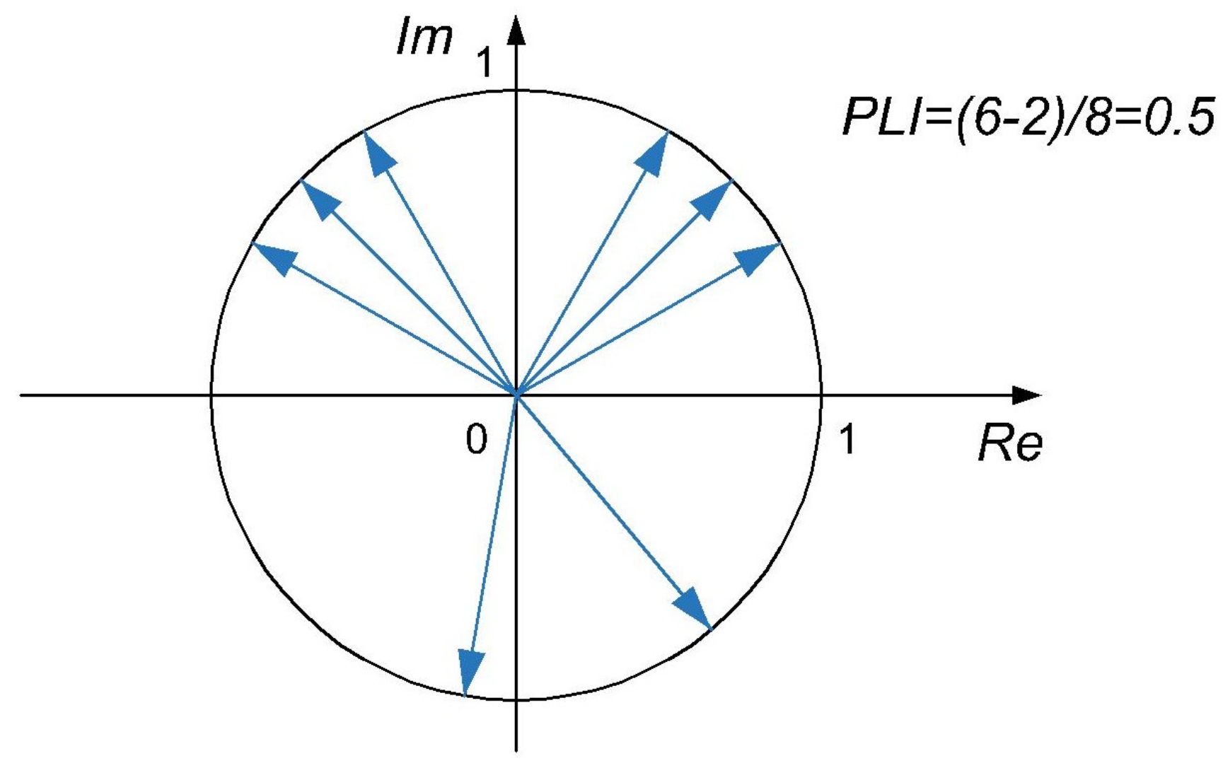
where and are the instantaneous amplitudes of the observed signals and at sample n. Based on Equation (9) and as shown in, Computation of PLI is illustrated in Figure 2. All unit vectors that represent phase differences are first divided into two subsets: those with positive, and those with negative imaginary part. Then, the difference of subsets’ sizes is divided by the number of all vectors N, and its absolute value equals the PLI.
Therefore, if there is a predominant positive or negative phase difference throughout the observed time interval, then the obtained value of PLI will be close or equal to 1. On the contrary, PLI which equals 0 is obtained when half of the phase differences are negative and the other half of them are positive.
The weighted phase lag index (wPLI) is an improved version of the phase lag index connectivity measure. The unit vectors of phase differences from PLI are now scaled with instantaneous amplitudes of both signals [19]. In other words, wPLI is obtained by weighting PLI with the imaginary part of the cross spectral density:
By expressing the cross spectral density from Equation (10) using the complex conjugate operator, the wPLI can be rewritten as follows:
which can be further simplified as:
Now we can show its relationship to the CPCC or more specifically to its imaginary part, denoted imCPCC:
Comparing Equations (14) and (15) we see that both measures, wPLI and imCPCC, are based on the imaginary part of the cross spectral density S in the numerator, and differ only in scaling in the denominator. The wPLI is scaled using the imaginary part of S only, while imCPCC with the power of both signals.
2.4. Connectivity Estimation Based on Phase Difference Histograms
In this section, we explain how connectivity reflects in phase difference histograms, to illustrate the connectivity measures. Although statistical properties of the phase difference distribution can clearly indicate phase locking of the signals [25], in practice, connectivity measures are rarely explained in these terms. We will use it to gain better insight into real connectivity between signals, particularly for the cases where values of connectivity measures are the highest or most different between each other.
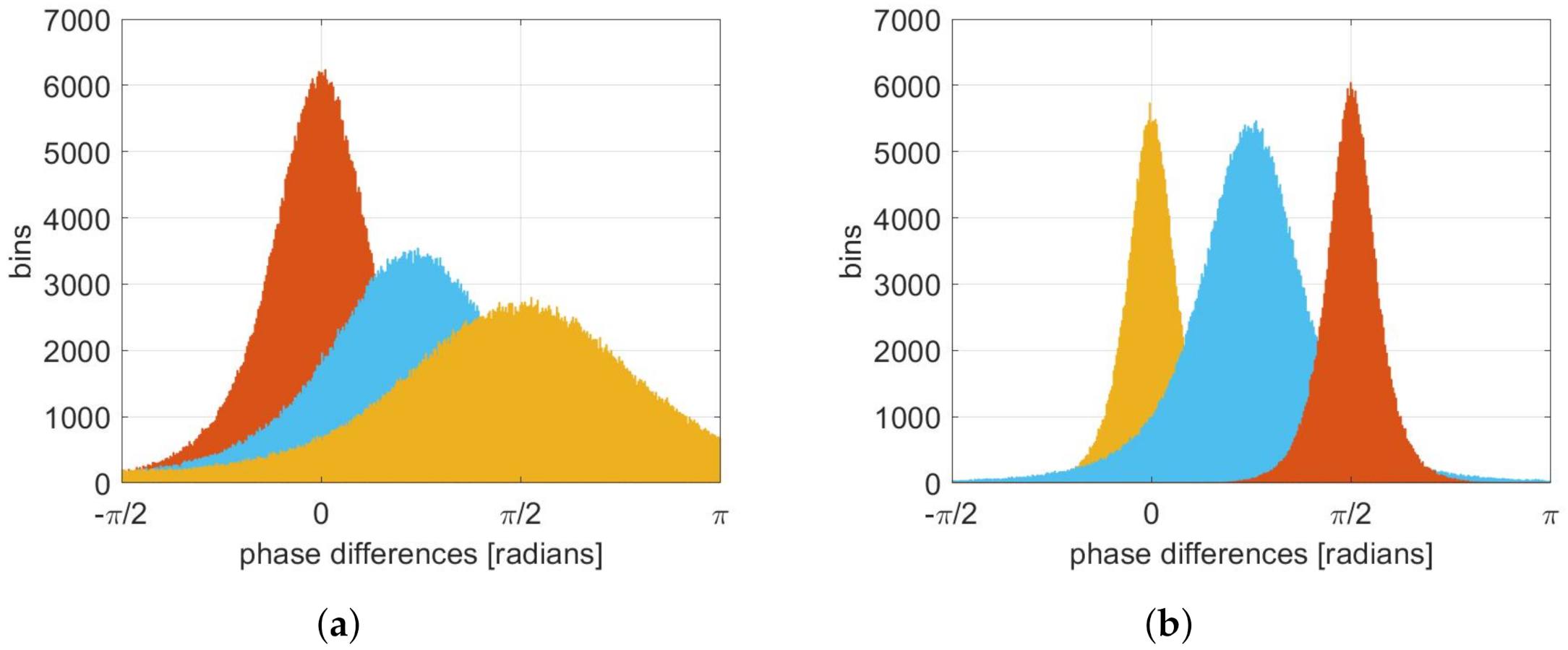
Let us first assume no volume conduction is present. When two signals are not connected, they change independently and the phase differences are uniformly distributed. Connectivity between two brain regions reflect in more expressed phase differences of corresponding signals. The higher the connectivity, the more pronounced the extreme gets, and the standard deviation of the distribution gets lower, see Figure 3a. The “red” distribution reflects the highest connectivity and its standard deviation is the lowest. On the other hand, the “orange” distribution has the highest standard deviation and reflects the lowest connectivity. The mean value of the phase distribution equals the average phase difference, and can have an arbitrary value in the range, and it does not depend on the connectivity level.
If volume conduction is present, certain signal components are included in both of the signals under consideration. These signal components have a phase difference of 0 or , but due to noise and signal interference, instantaneous phase differences spread around these values. These values therefore do not (necessarily) imply higher connectivity. In the example in Figure 3b, we can expect that distributions with peaks closer to are more likely to reflect volume conduction and not connectivity. The estimated connectivity is therefore the highest when the value at 0 and is the lowest and the variance the smallest.
3. Results
In this section, we compare the proposed CPCC measures with PLV and wPLI using synthetic signals and real-life signals from freely available datasets.
3.1. Synthetic Signals from the MRC Brain Network Dynamics Unit (University of Oxford)
In the first experiment, we generated synthetic signals following Mäkinen et al. [26]. The EEG data we generated contained 31 channels from 973 trials, which were concatenated into a single large signal. This suited our particular purpose, as we analyzed general brain connectivity independent of specific brain events.
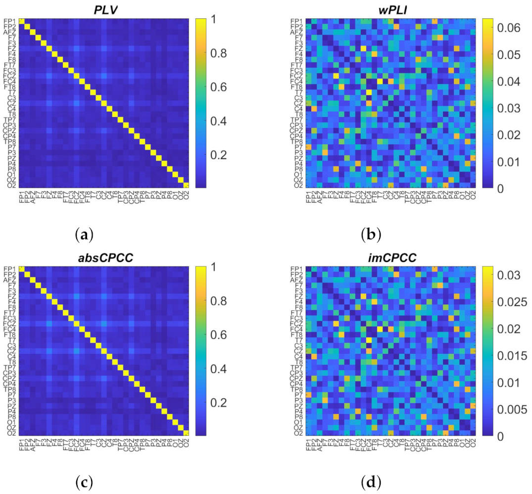
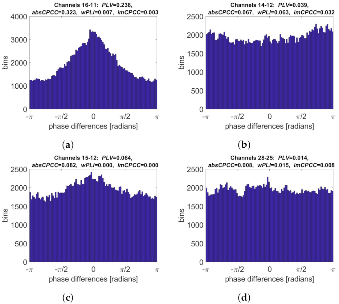
We computed connectivity using the proposed and established methods for different frequency bands. The connectivity matrices representing the estimated connectivity for each electrode pair and for all four measures are shown in Figure 4. We can clearly see strong visual similarities between the proposed measures and the most commonly used measures, i.e., between PLV and absCPCC, as well as wPLI and imCPCC.
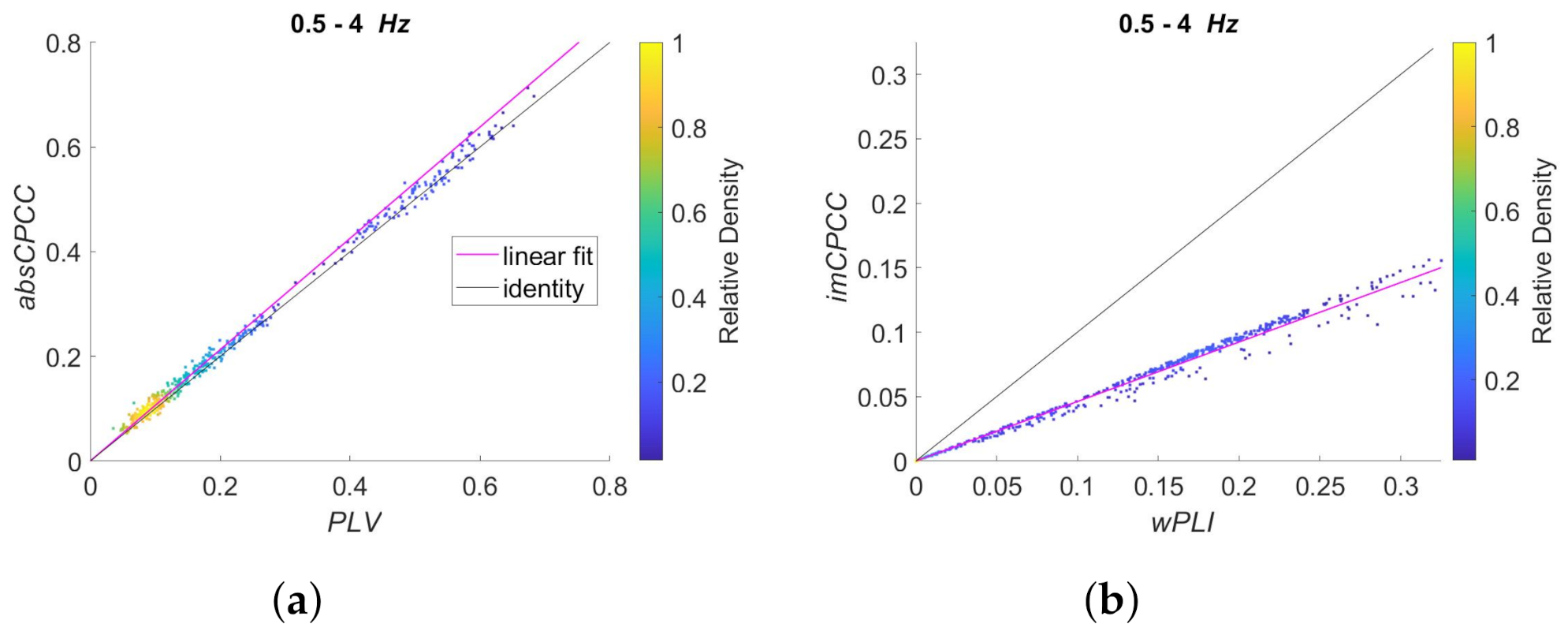
To better compare the connectivity measures, see Figure 5, with scatter plots for measure pairs PLV to absCPCC and wPLI to imCPCC. Each dot in a scatter plot represents one electrode pair. The color of the dots depends on the relative density of the dots in the graph. There are also two lines shown, where the black one represents identity while the cyan one the best linear fit. High correlation is evident for both connectivity measure pairs, while the scaling differences depend on the frequency band, most evidently for the PLV to absCPCC pair. There are some electrode pairs that deviate slightly from the general linear relationship while the overall correlation of the measures seem to be high.
To evaluate the relationship between the measures, evident from Figure 5, we computed their correlation. In addition to frequency bands shown in Figure 5, 0.5–4 Hz, 4–8 Hz and 8–13 Hz, we computed it for 13–18, 18–30, and 35–45 Hz frequency bands. For all the frequency bands and both pairs, i.e., PLV to absCPCC, and wPLI to imCPCC; the obtained correlation equaled , proving the close to perfect relationship between the measures.
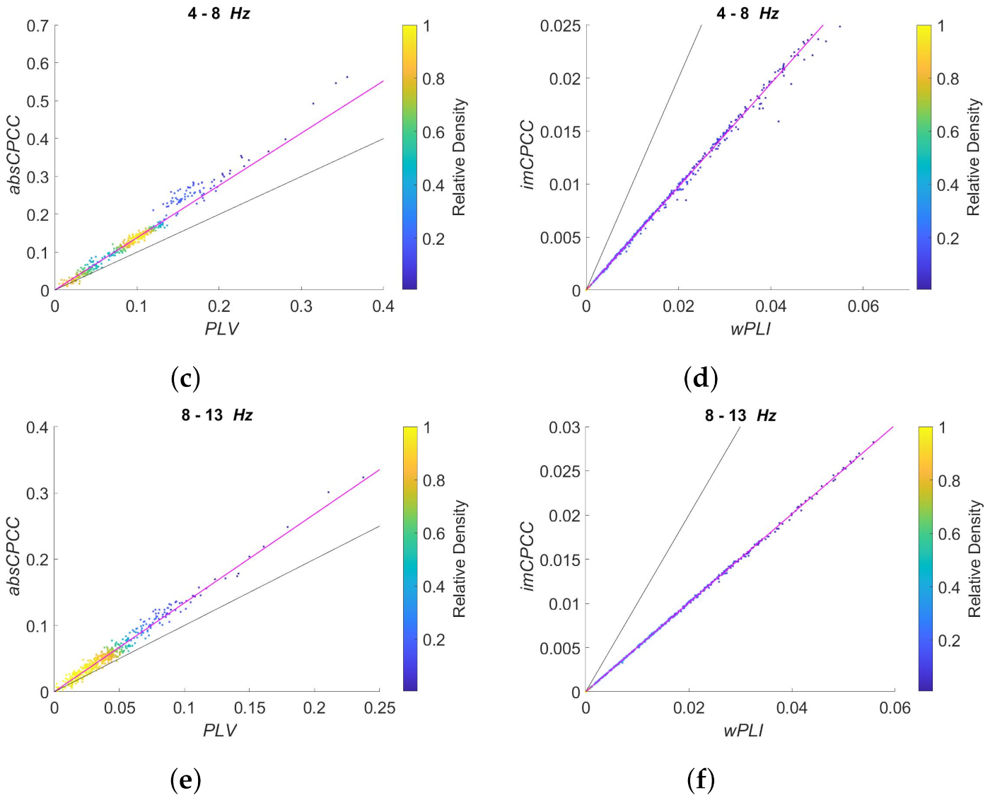
Finally, we selected electrode pairs with the highest connectivity values and the highest ratio between them. Their phase difference distributions are shown in Figure 6. As expected, the same electrode pair (16–11) had the highest PLV and absCPCC values. The corresponding phase distribution was centered at the phase angle 0, indicating the possibility of volume conduction. Similarly, one electrode pair (14–12) had the highest in both wPLI and imCPCC values. The corresponding phase distribution has a less pronounced peak off the center. The ratios between PLV and wPLI, as well as absCPCC and imCPCC values, were the highest when the later ones equalled 0 and the histogram was centered (electrode pair 15–12). The highest and wPLI to PLV ratio and imCPCC to absCPCC ratio were obtained when absCPCC equaled imCPCC.
3.2. Synthetic Signals Generated with the Kuramoto Model
The second set of synthetic signals to test connectivity estimation methods was generated using the Kuramoto model according to [27]. The reason for using it is that the relationship between electrodes is defined and known in advance. Twenty-four signals (channels/electrodes) were generated. The signals form three groups, from 1 to 8, 9 to 16, and 17 to 24. They are composed of two signal components, where the first component is synchronized between all electrodes in a group and the second component is not synchronized and gives a more realistic variability to the signal set. The signals from 17 to 24 are composed of the first components only and due to the high coupling factor (K = 1000), these signals are synchronized very quickly. As a result of the fast synchronization, these signals are in phase and can be observed as an example of high volume conduction.
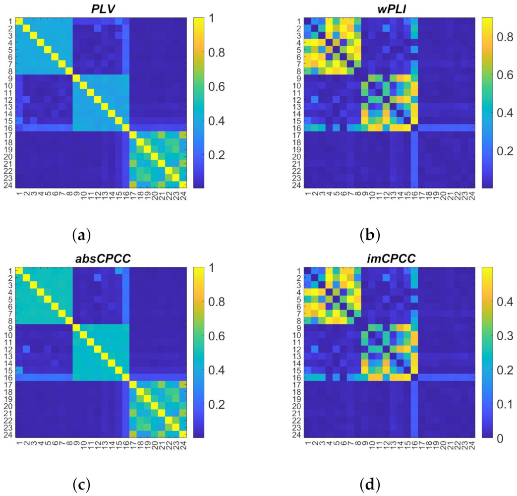
Figure 7 shows the connectivity matrices of the observed connectivity measures. It is visible that the signals are connected within groups and much less between the groups. The random nature of the generation process could lead to synchronous signals even between different groups. Looking at the third group of signals, we also see a tendency for the PLV and absCPCC to include volume conduction as an acceptable contribution to the connectivity, while wPLI and imCPCC avoid this component.
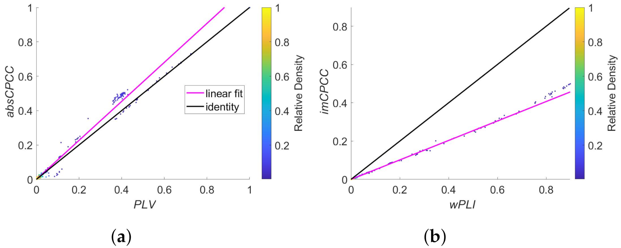
In Figure 8 is a scatter plot showing the relationship between absCPCC and PLV values (a) and between the imCPCC and wPLI values (b). A strong linear relationship is evident for both connectivity estimation method pairs, while the scaling is different.
The correlation between PLV and absCPCC values as well as the correlation between wPLI and imCPCC equals , indicating strong similarities between these measures.
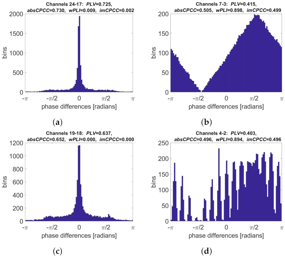
The phase difference distributions for signal pairs with the highest connectivity values and the highest ratio between them are shown in Figure 9. The phase difference distribution corresponding to the highest PLV and absCPCC values was narrow and centered around 0. It was obtained for two signals from the last group (24–17), which modeled volume conduction. The highest wPLI and imCPCC values were obtained for signals from the first group (7–3), with wide distribution centered at radians. The ratio between the absCPCC and imCPCC values was the highest when the latter one equaled 0 and the histogram was centered, indicating possible volume conduction (signal pair 19–18). The highest imCPCC to absCPCC ratio was, again, obtained when values for both measures were equal, with a clear peak of the distribution at radians.
3.3. Real-Life Signals
For testing on real-life data, we used the SPIS Resting State Dataset [28], a multimodal dataset with EEG and forehead EOG signals. In our analysis, we used only EEG signals from the “eyes closed” (EC) and “eyes open” (EO) states with a duration of 2.5 min, using 256 Hz sampling rate.
Offline preprocessing of the EEG signal was performed in the following sequence of steps:
- The raw brain activity data were imported into MATLAB using the EEGLAB toolbox;
- Electrode positions (also called channel locations) were defined in the software;
- The data were referenced to average;
- The data were filtered with a band pass filter limited to 0.5 and 45 Hz;
- Automatic spectral-based channel suppression (z = 5) was performed using the EEGLAB “pop rejchan” function;
- Artifacts were removed using the ICLabel plugin for EEGLAB (thresholds for removing components were less than or equal to 0.05 for brain activity and greater than or equal to 0.9 for artifacts);
- The data were re-referenced to average;
- Sub-bands of the EEG signal were extracted (delta 0.5–4 Hz, theta 4–8 Hz, alpha 8–13 Hz, low beta 13–18 Hz, high beta 18–30 Hz, gamma 35–45 Hz).
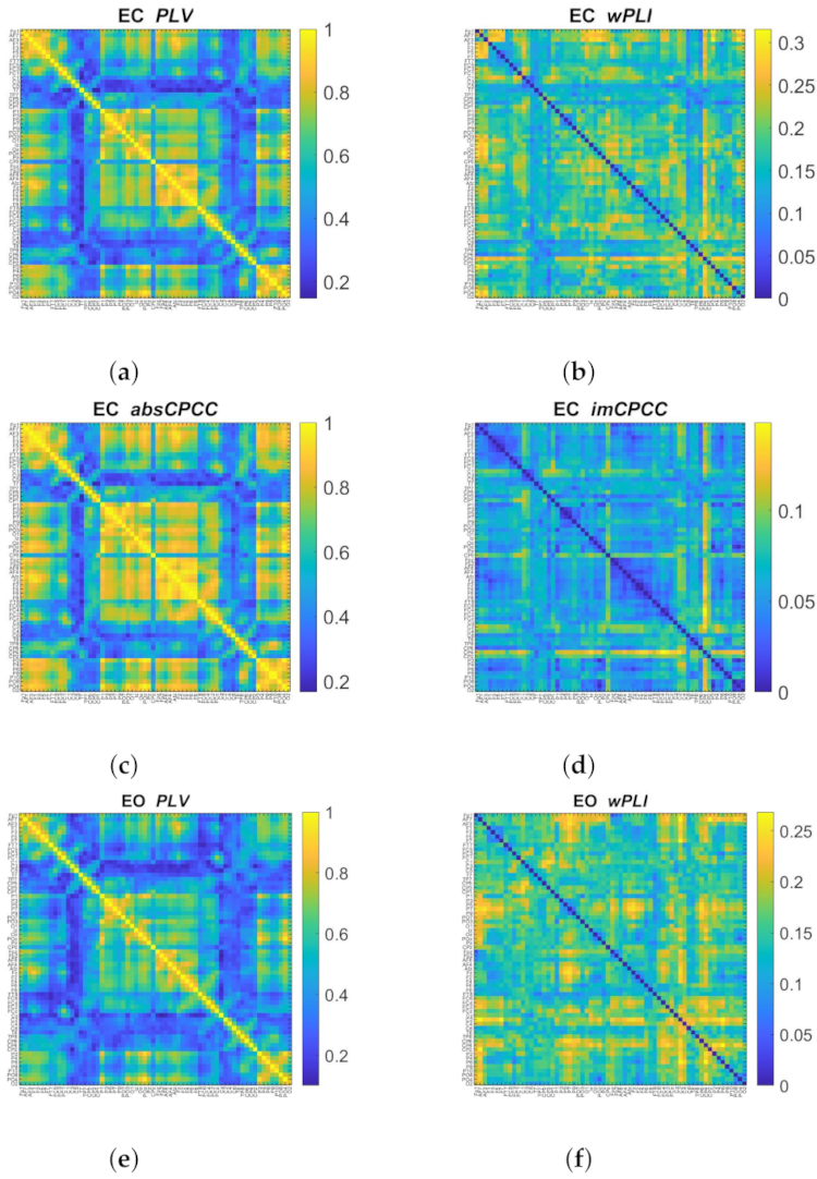
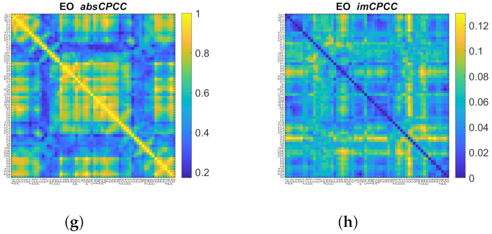
Figure 10 shows the connectivity matrices for PLV, absCPCC, wPLI, and imCPCC for both conditions (EC and EO) in the alpha band (8–13 Hz). The similarity between PLV and absCPCC, as well as between wPLI and imCPCC, is visible, although with some evident differences, mainly between the latter two. Although the patterns are similar, the color scaling (based on the highest value) is different.
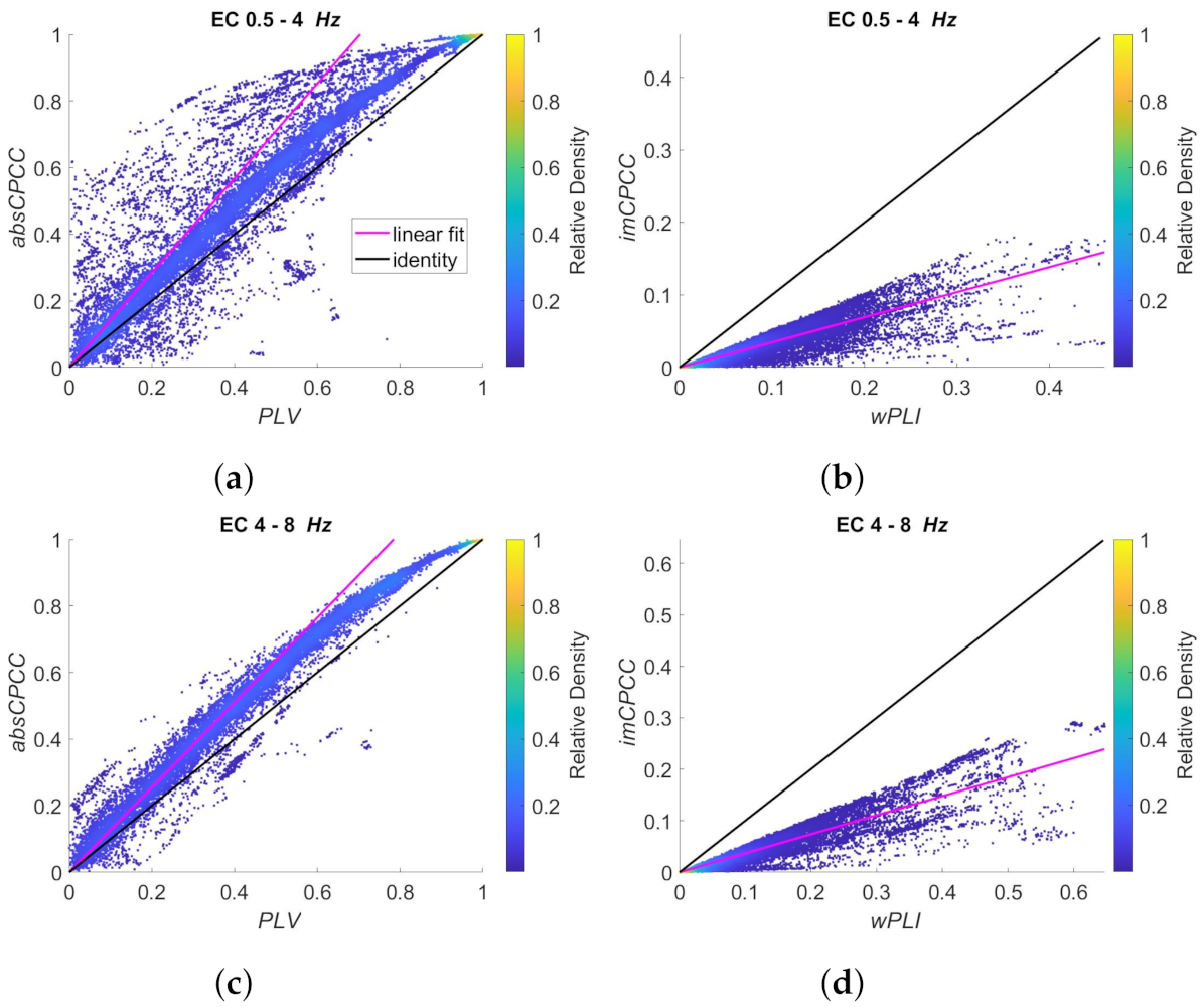
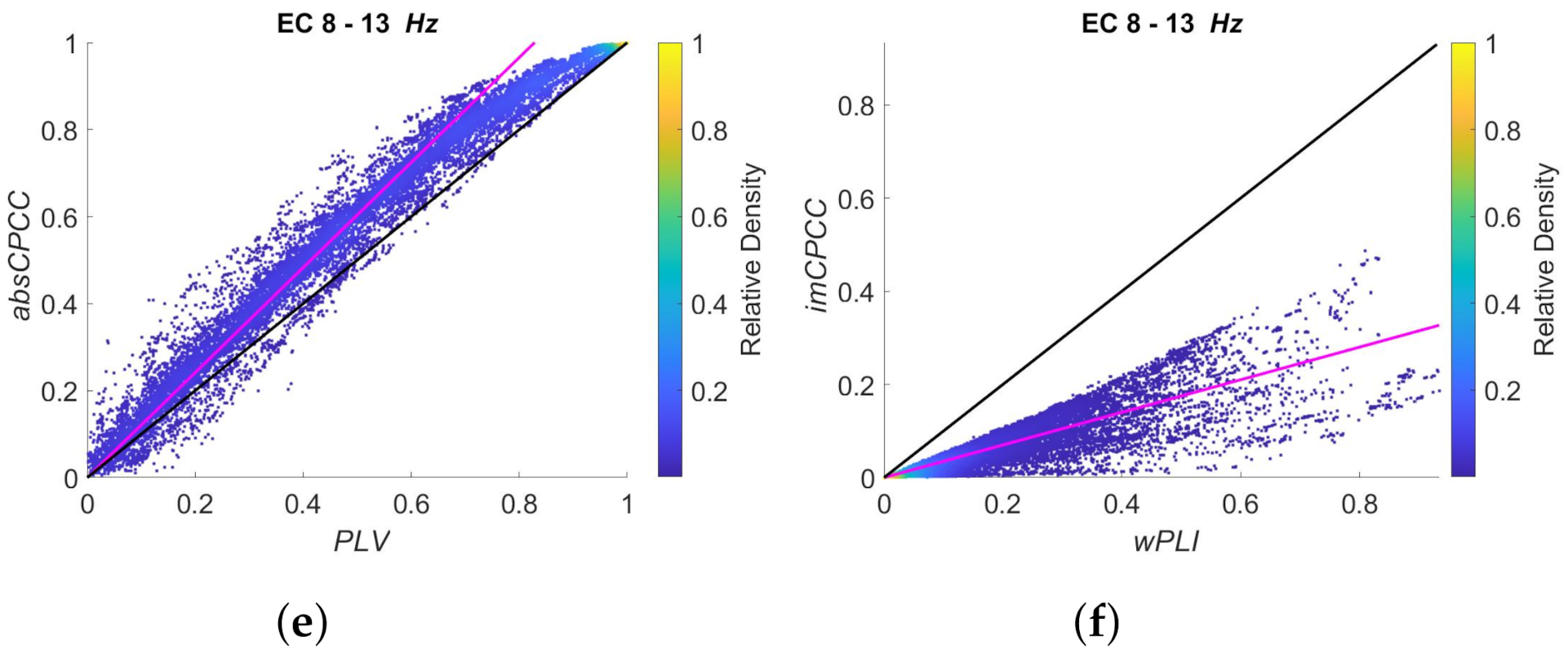
Figure 11 and Figure 12 show the relationship between absCPCC and PLV values (left) and between the imCPCC and wPLI values (right) for all the frequency ranges. Figure 11 shows the signals recorded with eyes closed (EC state), while Figure 12 is for eyes open (EO state). We can see that absCPCC and PLV as well as imCPCC and wPLI are positively correlated in all frequency bands. However, we have to be aware that real-life signals include multiple signal components with different amplitudes, while the scaling is common for the whole sequence. This makes the results more scattered in PLV-absCPCC and wPLI-imCPCC distributions. The relationship between absCPCC and PLV is evident, but with visible deviation from being perfectly linear due to reduced scaling difference for high connectivity values. The relationship between imCPCC and wPLI also deviates from linear, with evident range of scaling differences. The relationships do not seem to be dependent on the EC/EO state.
To enumerate the linearity of relationships between the connectivity measures, we show the correlation values between them in Table 1.
The correlation between absCPCC and PLV connectivity measures is high for all frequency bands and both states (EC and EO), with an average of . Only slightly lower values are obtained for the correlation between imCPCC and wPLI, with an average of . The corresponding p-values for the alternative hypothesis that measures are not correlated are all smaller than 0.0001 and, thus, well below the significance level of 0.05, which means that the hypothesis of the correlation between the absCPCC and PLV and between imCPCC and wPLI is proven for all frequency bands and both states.
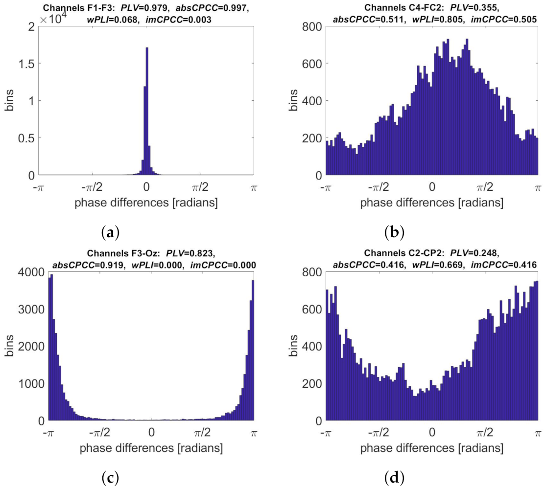
Phase difference distributions for real-life signals for electrode pairs with the highest connectivity values and the highest ratios between them are shown in Figure 13. The phase difference distributions corresponding to the highest PLV and absCPCC values are narrow and centered around 0. The highest wPLI and imCPCC values are obtained when the distribution that is wide, slightly asymmetric, and centered at non-zero phase difference. The ratio between absCPCC and imCPCC values is the highest when the later one equal 0 and the histogram is centered at radians. The highest imCPCC to absCPCC ratio is, again, obtained when their values are equal and the histogram is not symmetric around 0.
4. Discussion and Conclusions
In this paper, we shed new light on the Pearson correlation for the EEG connectivity analysis. We introduced the complex correlation (CPCC) as a measure of brain connectivity. We compared it to the (currently) most widely used brain connectivity measures, i.e., PLV [17,18] and wPLI [19]. The correlation coefficient (CC) has been used before, but only between the real signals, not the analytic ones, and it was shown that it does not represent the optimal metric to estimate functional interactions [29]. It equals the real component of CPCC, while we showed the importance of the absolute value and the imaginary component of CPCC.
We showed that the imaginary part of the complex Pearson correlation (imCPCC) is closely related to the wPLI measure and that the absolute value of the complex Pearson correlation absCPCC is closely related to PLV. The relationships are proven analytically and numerically, on two types of synthetic signals [26,27] and on real-life EEG signals [28]. Analytically, the differences are only in the denominators that are normalizing the measures to the interval. Numerically, high correlations between the results obtained with related measures are shown. For synthetic signals, the correlation level is for all frequency bands equal to . The scaling differences are evident for absCPCC to PLV relationship, and differ for different frequency bands. The connectivity results for real-life signals show more differences and the measures are less correlated, but still with an average correlation of for absCPCC to PLV relationship and for the imCPCC to wPLI relationship. Real-life signals consist of more components, which originate in different sources, are related through different neural paths, and include different (although similar) frequencies. Even when limiting frequency bandwidths, they are more information-rich than simulated signals. Connectivity could be understood as a portion of signal components that affects two distinct electrode signals, but can vary with time. All of this reflects in more complex phase difference histograms and more complex scatter-plotted relationships between the measures.
Based on the results shown in this paper, and the fact that connectivity measures are currently typically analyzed relatively, we conclude that PLV can be replaced with absCPCC and wPLI with imCPCC. Moreover, the absCPCC and imCPCC measures are defined as two components of the the same CPCC measure and are, therefore, related, while PLV and wPLI are not. This enables comparison of the connectivity components that may be affected by volume conduction and those which are certainly not. The imaginary component of CPCC can only be lower or equal to the absolute CPCC value due to the excluded real CPCC component, which depends on signal components that may result from volume conduction. It can be expected that the true connectivity may also yield in-phase signals of two electrodes, which makes them indistinguishable from volume conduction. Similar to wPLI, imCPCC scales the components, such that ones more likely arise from volume conduction have lower influence. Thus, the estimated connectivity deviates from the true one, but CPCC provides the upper and lower boundary, with absCPCC and imCPCC respectively. Neuroscientists sometimes have a practice of calculating both the PLV and wPLI (or PLI) and then interpreting the results [29,30,31,32] because the PLV method, unlike the wPLI, does not take into account the influence of volume conduction. With the proposed CPCC measures, they can get additional information, related to the ratio of both connectivity components. As such, the CPCC measure could be used for various neurology related studies. Such studies include the EEG-based brain mechanism of sleep stages, which is important for sleep quality assessment and disease diagnosis [33]. By averaging over the trial set, the proposed measures could also be used as a solution to improve the prediction results of the phases of the synchronization and desynchronization tasks [34]. The potential application of CPCC also lies in the assessment of mental stress levels using functional connectivity as a parameter [35,36] and in the diagnosis dyslexia [37]. In addition, the proposed measures could be used as parameters for the evaluation of simulated EEG data based on the theory of functional connectivity of the brain [38].
The next valuable property of the proposed CPCC measure is that it can be computed as a summation of temporal sample contributions. This enables the measure to reveal temporal changes of connectivity and opens a new direction for further research. This can be especially useful for analyzing human brain networks in auditory and visual tasks [39,40] and is also promising for assessing motor skills [41]. This also allows us to observe changes in the organization of brain network connectivity over time using well-known measures from complex network graph theory [42].
The CPCC measure has an advantage in the computational complexity. In our experiments the computation of absCPCC and imCPCC was to faster than the computations of PLV and wPLI.
Finally, the computation of the correlation of two analytic signals is easy to implement and already available in most of the statistical and signal analysis tools.
Following the above discussion—we can state that the newly proposed CPCC connectivity measure, with absCPCC and imCPCC as its components, could replace PLV and wPLI measures, accelerate the computation of brain connectivity, and provide further information about brain processes. The data, code, and instructions for replicating the study presented in this article are freely available at https://github.com/zsverko/Code_CPCC.git (accessed on 10 January 2022).
Author Contributions
Conceptualization, S.V. and P.R.; methodology, S.V., P.R. and Z.Š.; software, Z.Š. and P.R.; validation, Z.Š. and P.R.; formal analysis, Z.Š.; investigation, Z.Š.; resources, M.V. and P.R.; data curation, Z.Š.; writing—original draft preparation, Z.Š. and P.R.; writing—review and editing, Z.Š., P.R., S.V. and M.V.; visualization, Z.Š.; supervision, P.R., S.V. and M.V.; project administration, Z.Š.; funding acquisition, Z.Š., S.V. and M.V. All authors have read and agreed to the published version of the manuscript.
Funding
This research received no external funding.
Institutional Review Board Statement
Not applicable.
Informed Consent Statement
Not applicable.
Data Availability Statement
The data, code, and instructions are freely available at https://github.com/zsverko/Code_CPCC.git (accessed on 10 January 2022).
Conflicts of Interest
The authors declare no conflict of interest.
Abbreviations
The following abbreviations are used in this manuscript:
| absCPCC | absolute value of complex Pearson correlation coefficient |
| CPCC | complex Pearson correlation coefficient |
| DTI | diffusion tensor imaging |
| EC | eyes closed |
| EEG | electroencephalography |
| EO | eyes open |
| HT | Hilbert transform |
| imCPCC | imaginary component of complex Pearson correlation coefficient |
| MEG | magnetoencephalography |
| MRI | magnetic resonance imaging |
| PLV | phase locking value |
| PLI | phase lag index |
| wPLI | weighted phase lag index |
References
- Fornito, A.; Zalesky, A.; Bullmore, E. Fundamentals of Brain Network Analysis, 1st ed.; Academic Press: London, UK, 2016; pp. 1–3. [Google Scholar]
- Sanei, S.; Chambers, J.A. EEG Signal Processing, 1st ed.; John Wiley & Sons: Hoboken, NJ, USA, 2016; pp. 1–8. [Google Scholar]
- Olejarczyk, E.; Marzetti, L.; Pizzella, V.; Zappasodi, F. Comparison of connectivity analyses for resting state EEG data. J. Neural Eng. 2017, 14, 036017. [Google Scholar] [CrossRef] [PubMed]
- Koch, M.A.; Norris, D.G.; Hund-Georgiadis, M. An investigation of functional and anatomical connectivity using magnetic resonance imaging. Neuroimage 2002, 16, 241–250. [Google Scholar] [CrossRef] [PubMed] [Green Version]
- Rose, S.; Pannek, K.; Bell, C.; Baumann, F.; Hutchinson, N.; Coulthard, A.; McCombe, P.; Henderson, R. Direct evidence of intra- and interhemispheric corticomotor network degeneration in amyotrophic lateral sclerosis: An automated MRI structural connectivity study. Neuroimage 2012, 59, 2661–2669. [Google Scholar] [CrossRef] [PubMed]
- Lim, S.; Han, C.E.; Uhlhaas, P.J.; Kaiser, M. Preferential detachment during human brain development: Age-and sex-specific structural connectivity in diffusion tensor imaging (DTI) data. Cereb. Cortex 2015, 25, 1477–1489. [Google Scholar] [CrossRef] [Green Version]
- Singer, W. Neuronal synchrony: A versatile code for the definition of relations? Neuron 1999, 24, 49–65. [Google Scholar] [CrossRef] [Green Version]
- Varela, F.; Lachaux, J.P.; Rodriguez, E.; Martinerie, J. The brainweb: Phase synchronization and large-scale integration. Nat. Rev. Neurosci. 2001, 2, 229–239. [Google Scholar] [CrossRef]
- Fries, P. A mechanism for cognitive dynamics: Neuronal communication through neuronal coherence. Trends Cogn. Sci. 2005, 9, 474–480. [Google Scholar] [CrossRef]
- Fries, P. Rhythms for cognition: Communication through coherence. Neuron 2015, 88, 220–235. [Google Scholar] [CrossRef] [Green Version]
- Siegel, M.; Donner, T.H.; Engel, A.K. Spectral fingerprints of large-scale neuronal interactions. Nat. Rev. Neurosci. 2012, 13, 121–134. [Google Scholar] [CrossRef]
- Bastos, A.M.; Schoffelen, J.M. A tutorial review of functional connectivity analysis methods and their interpretational pitfalls. Front. Syst. Neurosci. 2016, 9, 175. [Google Scholar] [CrossRef] [Green Version]
- Sakkalis, V. Review of advanced techniques for the estimation of brain connectivity measured with EEG/MEG. Comput. Biol. Med. 2011, 41, 1110–1117. [Google Scholar] [CrossRef]
- Hwa, R.C.; Ferree, T.C. Scaling properties of fluctuations in the human electroencephalogram. Phys. Rev. E 2002, 66, 021901. [Google Scholar] [CrossRef] [Green Version]
- Li, L.; Zhang, J.X.; Jiang, T. Visual working memory load-related changes in neural activity and functional connectivity. PLoS ONE 2011, 6, e22357. [Google Scholar] [CrossRef] [Green Version]
- Stam, C.J.; Van Dijk, B.W. Synchronization likelihood: An unbiased measure of generalized synchronization in multivariate data sets. Phys. D 2002, 163, 236–251. [Google Scholar] [CrossRef]
- Stam, C.J.; Nolte, G.; Daffertshofer, A. Phase lag index: Assessment of functional connectivity from multi channel EEG and MEG with diminished bias from common sources. Hum. Brain Mapp. 2007, 28, 1178–1193. [Google Scholar] [CrossRef]
- Lachaux, J.P.; Rodriguez, E.; Martinerie, J.; Varela, F.J. Measuring phase synchrony in brain signals. Hum. Brain Mapp. 1999, 8, 194–208. [Google Scholar] [CrossRef] [Green Version]
- Vinck, M.; Oostenveld, R.; Van Wingerden, M.; Battaglia, F.; Pennartz, C.M. An improved index of phase-synchronization for electrophysiological data in the presence of volume-conduction, noise and sample-size bias. Neuroimage 2011, 55, 1548–1565. [Google Scholar] [CrossRef]
- Schreier, P.J. A unifying discussion of correlation analysis for complex random vectors. IEEE Trans. Signal Process 2008, 56, 1327–1336. [Google Scholar] [CrossRef]
- Ma, G.; Li, L. Depth and structural index estimation of 2D magnetic source using correlation coefficient of analytic signal. J. Appl. Geophys. 2013, 91, 9–13. [Google Scholar] [CrossRef]
- Fuhrmann, D.R.; San Antonio, G. Transmit beamforming for MIMO radar systems using signal cross-correlation. IEEE Trans. Aerosp. Electron. Syst. 2008, 44, 171–186. [Google Scholar] [CrossRef]
- Makita, S.; Kurokawa, K.; Hong, Y.J.; Miura, M.; Yasuno, Y. Noise-immune complex correlation for optical coherence angiography based on standard and Jones matrix optical coherence tomography. Biomed. Opt. Express 2016, 7, 1525–1548. [Google Scholar] [CrossRef] [Green Version]
- Welch, P. The use of fast Fourier transform for the estimation of power spectra: A method based on time averaging over short, modified periodograms. IEEE Trans. Audio Electroacoust. 1967, 15, 70–73. [Google Scholar] [CrossRef] [Green Version]
- Tass, P.; Rosenblum, M.G.; Weule, J.; Kurths, J.; Pikovsky, A.; Volkmann, J.; Schnitzler, A.; Freund, H.J. Detection of n:m Phase Locking from Noisy Data: Application to Magnetoencephalography. Phys. Rev. Lett. 1998, 81, 3291–3294. [Google Scholar] [CrossRef]
- Mäkinen, V.; Tiitinen, H.; May, P. Auditory event-related responses are generated independently of ongoing brain activity. NeuroImage 2005, 24, 961–968. [Google Scholar] [CrossRef]
- Šverko, Z.; Sajovic, J.; Drevenšek, G.; Vlahinić, S.; Rogelj, P. Generation of Oscillatory Synthetic Signal Simulating Brain Network Dynamics. In Proceedings of the 2021 44th International Convention on Information, Communication and Electronic Technology (MIPRO), MEET—Microelectronics, Electronics and Electronic Technology, Opatija, Croatia, 27 September–1 October 2021. [Google Scholar]
- Torkamani Azar, M.; Kanik, S.D.; Aydin, S.; Cetin, M. Prediction of reaction time and vigilance variability from spatio-spectral features of resting-state EEG in a long sustained attention task. IEEE J. Biomed. Health Inform. 2020, 24, 2550–2558. [Google Scholar] [CrossRef] [Green Version]
- Fraschini, M.; Pani, S.M.; Didaci, L.; Marcialis, G.L. Robustness of functional connectivity metrics for EEG-based personal identification over task-induced intra-class and inter-class variations. Pattern Recognit. Lett. 2019, 125, 49–54. [Google Scholar] [CrossRef]
- Hardmeier, M.; Hatz, F.; Bousleiman, H.; Schindler, C.; Stam, C.J.; Fuhr, P. Reproducibility of functional connectivity and graph measures based on the phase lag index (PLI) and weighted phase lag index (wPLI) derived from high resolution EEG. PLoS ONE 2014, 9, e108648. [Google Scholar] [CrossRef] [Green Version]
- Hu, L.; Zhang, Z. EEG Signal Processing and Feature Extraction; Springer: Singapore, 2019; pp. 241–266. [Google Scholar]
- Sarmukadam, K.; Bitsika, V.; Sharpley, C.F.; McMillan, M.M.; Agnew, L.L. Comparing different EEG connectivity methods in young males with ASD. Behav. Brain Res. 2020, 383, 112482. [Google Scholar] [CrossRef]
- Huang, H.; Zhang, J.; Zhu, L.; Tang, J.; Lin, G.; Kong, W.; Lei, X.; Zhu, L. EEG-Based Sleep Staging Analysis with Functional Connectivity. Sensors 2021, 21, 1988. [Google Scholar] [CrossRef]
- Caicedo-Acosta, J.; Castaño, G.A.; Acosta-Medina, C.; Alvarez-Meza, A.; Castellanos-Dominguez, G. Deep Neural Regression Prediction of Motor Imagery Skills Using EEG Functional Connectivity Indicators. Sensors 2021, 21, 1932. [Google Scholar] [CrossRef]
- Hag, A.; Handayani, D.; Pillai, T.; Mantoro, T.; Kit, M.H.; Al-Shargie, F. EEG Mental Stress Assessment Using Hybrid Multi-Domain Feature Sets of Functional Connectivity Network and Time-Frequency Features. Sensors 2021, 21, 6300. [Google Scholar] [CrossRef] [PubMed]
- Katmah, R.; Al-Shargie, F.; Tariq, U.; Babiloni, F.; Al-Mughairbi, F.; Al-Nashash, H. A Review on Mental Stress Assessment Methods Using EEG Signals. Sensors 2021, 21, 5043. [Google Scholar] [CrossRef]
- Formoso, M.A.; Ortiz, A.; Martinez-Murcia, F.J.; Gallego, N.; Luque, J.L. Detecting Phase-Synchrony Connectivity Anomalies in EEG Signals. Application to Dyslexia Diagnosis. Sensors 2021, 21, 7061. [Google Scholar] [CrossRef] [PubMed]
- Anzolin, A.; Toppi, J.; Petti, M.; Cincotti, F.; Astolfi, L. SEED-G: Simulated EEG Data Generator for Testing Connectivity Algorithms. Sensors 2021, 21, 3632. [Google Scholar] [CrossRef] [PubMed]
- Chikara, R.K.; Ko, L.-W. Modulation of the Visual to Auditory Human Inhibitory Brain Network: An EEG Dipole Source Localization Study. Brain Sci. 2019, 9, 216. [Google Scholar] [CrossRef] [PubMed] [Green Version]
- Perez-Ortiz, C.X.; Gordillo, J.L.; Mendoza-Montoya, O.; Antelis, J.M.; Caraza, R.; Martinez, H.R. Functional Connectivity and Frequency Power Alterations during P300 Task as a Result of Amyotrophic Lateral Sclerosis. Sensors 2021, 21, 6801. [Google Scholar] [CrossRef] [PubMed]
- García-Murillo, D.G.; Alvarez-Meza, A.; Castellanos-Dominguez, G. Single-Trial Kernel-Based Functional Connectivity for Enhanced Feature Extraction in Motor-Related Tasks. Sensors 2021, 21, 2750. [Google Scholar] [CrossRef]
- Vecchio, F.; Pappalettera, C.; Miraglia, F.; Alù, F.; Orticoni, A.; Judica, E.; Cotelli, M.; Pistoia, F.; Rossini, P.M. Graph Theory on Brain Cortical Sources in Parkinson’s Disease: The Analysis of ‘Small World’ Organization from EEG. Sensors 2021, 21, 7266. [Google Scholar] [CrossRef]
Figure 1.
Visualization of averaging used in calculation of the PLV. The PLV is computed from unit vectors representing instantaneous phase differences.
Figure 1.
Visualization of averaging used in calculation of the PLV. The PLV is computed from unit vectors representing instantaneous phase differences.

Figure 2.
Visualization of averaging used in calculation of the PLI. The PLI is computed from unit vectors representing instantaneous phase differences.
Figure 2.
Visualization of averaging used in calculation of the PLI. The PLI is computed from unit vectors representing instantaneous phase differences.

Figure 3.
The relationship between connectivity and phase differences distributions. When volume conduction is not considered (a) higher connectivity reflects in lower variance, while the mean value is irrelevant. In the presence of volume conduction (b), it reflects in higher values for phase differences close to 0 or , which, therefore, do not (necessarily) indicate connectivity. Connectivity level is expressed with colors; red is the highest and yellow is the lowest.

Figure 4.
Connectivity matrices obtained with PLV (a), wPLI (b), absCPCC (c), and imCPCC (d) for signals generated with [26], for 8–13 Hz frequency band.
Figure 4.
Connectivity matrices obtained with PLV (a), wPLI (b), absCPCC (c), and imCPCC (d) for signals generated with [26], for 8–13 Hz frequency band.

Figure 5.
Scatter plots of absCPCC to PLV relationship (left) and imCPCC to wPLI relationship (right). Each dot represents one electrode pair. Dots are colored according to their relative density. The black line represents identity, while the cyan one is the best linear fit. Rows correspond to different frequency bands: (a,b) 0.5–4 Hz; (c,d) 4–8 Hz; (e,f) 8–13 Hz.


Figure 6.
Phase difference distributions for selected electrode pairs (synthetic signals [26]). Shown are the distributions corresponding to the highest: (a) PLV and absCPCC values, (b) wPLI and imCPCC values, (c) ratio between absCPCC and imCPCC values, (d) ratio between imCPCC and absCPCC values.
Figure 6.
Phase difference distributions for selected electrode pairs (synthetic signals [26]). Shown are the distributions corresponding to the highest: (a) PLV and absCPCC values, (b) wPLI and imCPCC values, (c) ratio between absCPCC and imCPCC values, (d) ratio between imCPCC and absCPCC values.

Figure 7.
Connectivity matrices obtained with PLV, wPLI, absCPCC, and imCPCC for signals generated with the Kuramoto model [27].
Figure 7.
Connectivity matrices obtained with PLV, wPLI, absCPCC, and imCPCC for signals generated with the Kuramoto model [27].

Figure 8.
Relationships between absCPCC and PLV (a), and wPLI and imCPCC (b), shown as a scatter plot of values for all signal pairs where signals were generated with the Kuramoto model [27]. The black line represent the identity while the cyan line shows the best linear fit. The colors of the dots represent the relative density of the connectivity values.

Figure 9.
Phase difference distributions for selected synthetic signal pairs generated using the Kuramoto model [27]. Shown are the distributions corresponding to the highest: (a) PLV and absCPCC values, (b) wPLI and imCPCC values, (c) ratio between absCPCC and imCPCC values, (d) ratio between imCPCC and absCPCC values.

Figure 10.
Connectivity matrices for the the alpha band (8–13 Hz) of the real-life signals [28] for eyes closed (EC) and eyes open (EO) states, computed with PLV, wPLI, absCPCC (g), and imCPCC (h).
Figure 10.
Connectivity matrices for the the alpha band (8–13 Hz) of the real-life signals [28] for eyes closed (EC) and eyes open (EO) states, computed with PLV, wPLI, absCPCC (g), and imCPCC (h).


Figure 11.
Scatter plots of the absCPCC to PLV relationship (left) and the imCPCC to wPLI relationship (right), for all electrode pairs and for 10 test subjects (EC state). The black line represents the identity, while the cyan line shows the best linear fit. The colors of the dots represent the relative density of the connectivity values. Each row is shown for a different frequency band: (a,b) 0.5–4 Hz; (c,d) 4–8 Hz; (e,f) 8–13 Hz.


Figure 12.
Scatter plots of the absCPCC to PLV relationship (left) and the imCPCC to wPLI relationship (right), for all electrode pairs and for 10 test subjects (EO state). The black line represents the identity, while the cyan line shows the best linear fit. The colors of the dots represent the relative density of the connectivity values. Each row is shown for a different frequency band: (a,b) 0.5–4 Hz; (c,d) 4–8 Hz; (e,f) 8–13 Hz.

Figure 13.
Phase difference distributions for selected electrode pairs (real-life signals [28]). For each distribution, all four measures are calculated. The figure shows the electrode pair with the highest: (a) PLV and absCPCC values, (b) wPLI, and imCPCC values, (c) ratio between absCPCC and imCPCC values, (d) ratio between imCPCC and absCPCC values.


Table 1.
Correlation values between compared connectivity measures (real-life signal). Here, and denote and respectively.
Table 1.
Correlation values between compared connectivity measures (real-life signal). Here, and denote and respectively.
| Frequency | State-EC | State-EO | ||
|---|---|---|---|---|
| (Hz) | ||||
| 0.5–4 | 0.93 | 0.86 | 0.94 | 0.89 |
| 4–8 | 0.98 | 0.91 | 0.97 | 0.94 |
| 8–13 | 0.98 | 0.86 | 0.97 | 0.91 |
| 13–18 | 0.99 | 0.94 | 0.99 | 0.96 |
| 18–30 | 0.98 | 0.96 | 0.99 | 0.96 |
| 35–45 | 0.96 | 0.95 | 0.99 | 0.95 |
Publisher’s Note: MDPI stays neutral with regard to jurisdictional claims in published maps and institutional affiliations. |
© 2022 by the authors. Licensee MDPI, Basel, Switzerland. This article is an open access article distributed under the terms and conditions of the Creative Commons Attribution (CC BY) license (https://creativecommons.org/licenses/by/4.0/).
Share and Cite
MDPI and ACS Style
Šverko, Z.; Vrankić, M.; Vlahinić, S.; Rogelj, P. Complex Pearson Correlation Coefficient for EEG Connectivity Analysis. Sensors 2022, 22, 1477. https://doi.org/10.3390/s22041477
AMA Style
Šverko Z, Vrankić M, Vlahinić S, Rogelj P. Complex Pearson Correlation Coefficient for EEG Connectivity Analysis. Sensors. 2022; 22(4):1477. https://doi.org/10.3390/s22041477
Chicago/Turabian StyleŠverko, Zoran, Miroslav Vrankić, Saša Vlahinić, and Peter Rogelj. 2022. "Complex Pearson Correlation Coefficient for EEG Connectivity Analysis" Sensors 22, no. 4: 1477. https://doi.org/10.3390/s22041477
Note that from the first issue of 2016, this journal uses article numbers instead of page numbers. See further details here.