
A Novel Collision-Free Homotopy Path Planning for Planar Robotic Arms


 , ,
, ,
Abstract
:1. Introduction
2. Path Planning Using Homotopy-Based Formulations
2.1. Spherical-Path-Tracking Algorithm
2.2. Predictor–Corrector Algorithm
3. Proposed Scheme for Path Planning of Planar Arms
Workspace and C-Space
4. HPPM-PRA Procedure Steps
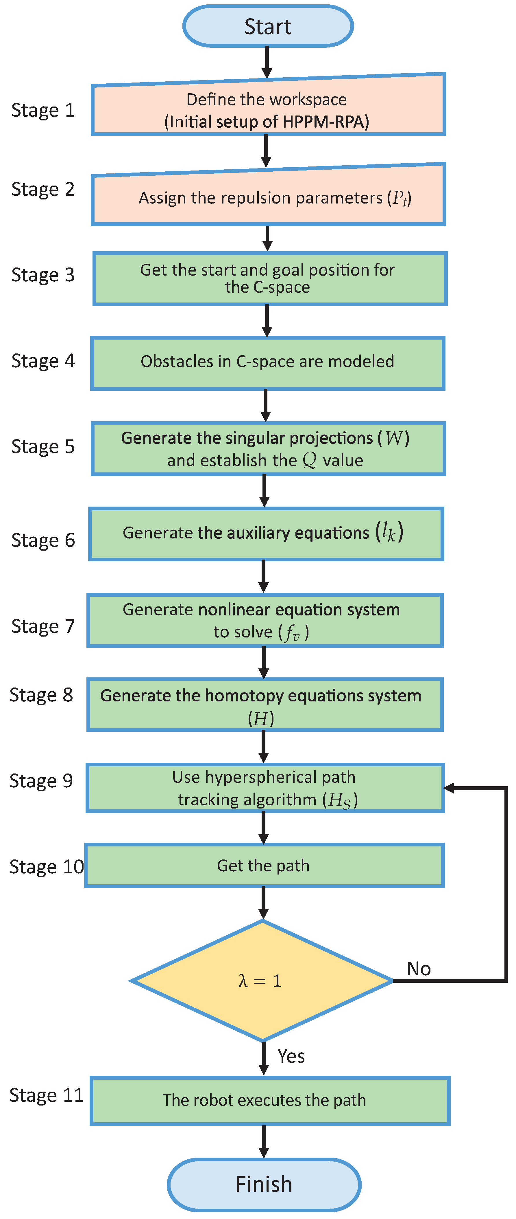
- 1.
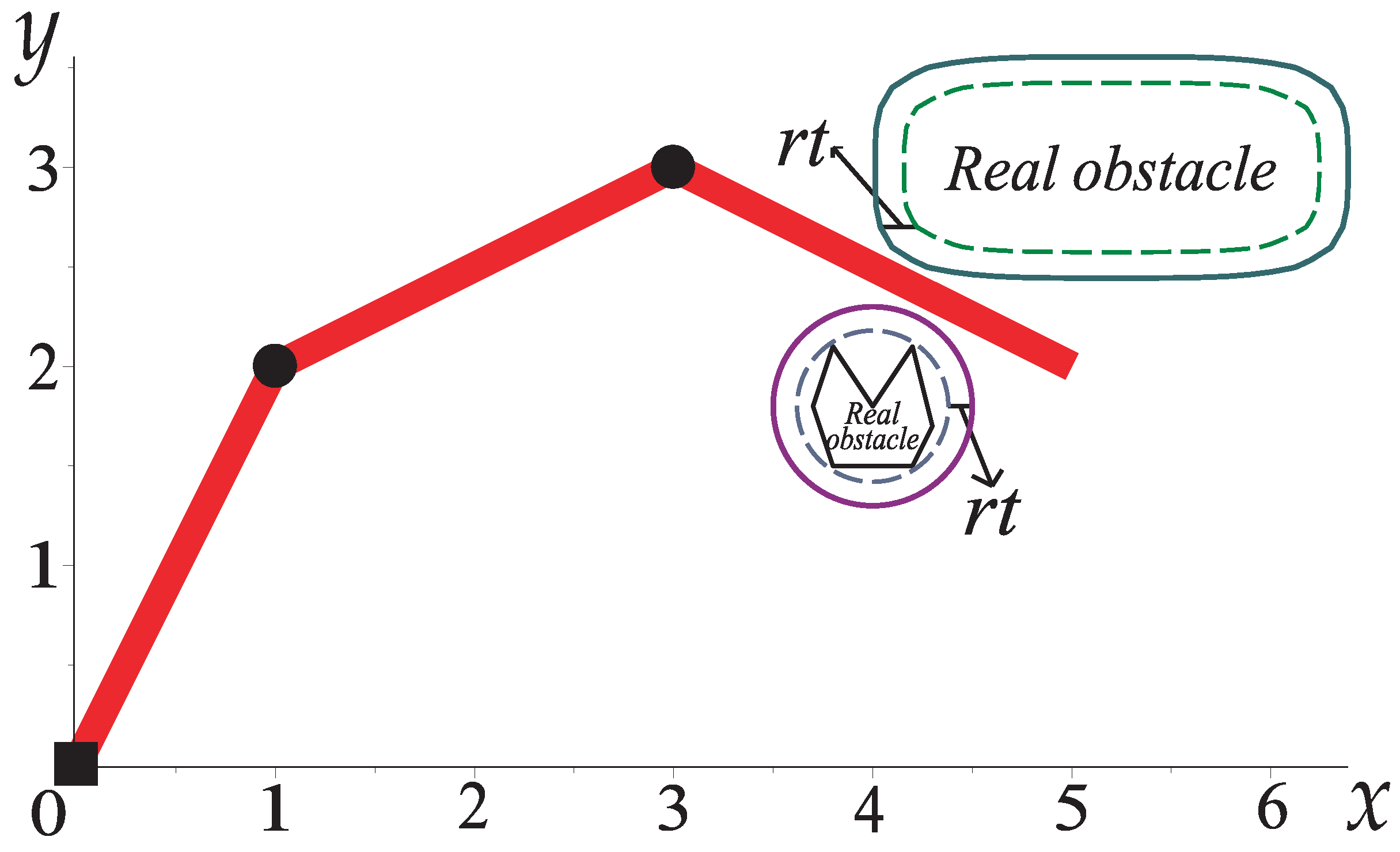
- Capturing of the workspace. In this step, a camera or system to capture the environment is used to generate the geometrical representation of the robot’s workspace. This procedure requires an image-processing algorithm; however, this is not a topic of this work; thus, the workspace is considered known a priori. Then, for this work, only circular obstacles (21) and ellipsoidal obstacles (22) are considered to represent the workspace in the case studies of Section 5.
- 2.
- Setting the robot parameters. The number and length of the links and the start and end configurations are given to the HPPM-PRA.
- 3.
- Repulsion parameter assignation. Assign the repulsion parameter to each obstacle of the workspace.
- 4.
- Model workspace obstacles in the C-space. The singular projections (W) that represent the forbidden configurations (obstacle collision space) are employed to establish the Q value using (23).
- 5.
- Generate the auxiliary equations. These are used to set the final configuration of the robotic arm.
- 6.
- Generate non-linear equation system. This represents the entire problem and contains the characteristics of the robot and the workspace.
- 7.
- Homotopy continuation formulation (Equation (26)). In this step, the original system of non-linear equations of the previous step is converted to a homotopic system.
- 8.
- Hyperspherical tracking. The hyperspherical tracking algorithm is employed to calculate each point of the solution path.
- 9.
- Robotic arm executing. Finally, the obtained homotopic path is followed by the robotic arm.
| Algorithm 1 HPPM-PRA general procedure. | |
| Require: , , | ▹ The task to be solved is proposed |
| Require: | ▹ Assign the repulsion parameter |
| 1: Get | ▹ See Algorithm 2 |
| 2: Get the value of Q | ▹ See Algorithm 3 |
| 3: Set the non-linear equation system to solve () | ▹ See Algorithm 4 |
| 4: Generate the homotopy equation (H) | ▹ See Algorithm 5 |
| 5: Create hypersphere | ▹ is used as the center of the first hypersphere |
| 6: Formulation of the homotopy system () | |
| 7: iteration=0 | ▹ A temporary variable is used as the counter |
| 8: whiledo | ▹ Use the hyperspherical path-tracking algorithm, until |
| 9: if then | |
| 10: Euler’s predictor () | ▹ Euler’s predictor is used |
| 11: else | |
| 12: Vector predictor () | ▹ The vector predictor is used |
| 13: end if | |
| 14: Broyden’s method () | ▹ The corrector method is used |
| 15: The numeric homotopy path is stored | |
| 16: Update the center of the hypersphere () | |
| 17: iteration++ | |
| 18: end while | |
| Ensure: The numerical homotopy path | ▹ The robotic arm can execute the path |
| Algorithm 2 Transformation from workspace to C-space. | |
| 1: functionC-space(, , ) | |
| 2: | ▹ Temporary variables |
| 3: for do | |
| 4: | ▹ Start position in C-space. |
| 5: | ▹ Goal position in C-space. |
| 6: end for | |
| 7: for do | ▹ Calculation of the value of . |
| 8: for do | |
| 9: | |
| 10: end for | |
| 11: | |
| 12: end for | |
| 13: return | ▹ Returns the values from the C-space |
| 14: end function |
| Algorithm 3 Get the value of (Q, W). | |
| 1: functionGet Q(,,,,,) | |
| 2: , | ▹ Temporal variables. |
| 3: for do | |
| 4: for do | |
| 5: for do | |
| 6: | |
| 7: | ▹ are the coordinates of each singular point for a given link |
| 8: | ▹ The equation of the circular obstacle can be replaced by the equation of ellipsoidal obstacle |
| 9: end for | |
| 10: | |
| 11: end for | |
| 12: | ▹ Temporal variable is cleared. |
| 13: | |
| 14: end for | |
| 15: return | ▹ The value of Q is obtained. |
| 16: end function |
| Algorithm 4 Set non-linear equation system to solve. | |
| 1: functionSet () | |
| 2: | ▹ Temporary variables |
| 3: for do | |
| 4: for do | |
| 5: | |
| 6: end for | |
| 7: | ▹ The system of auxiliary equations is obtained |
| 8: end for | |
| 9: for do | |
| 10: | |
| 11: end for | |
| 12: | |
| 13: return f | ▹ Returns |
| 14: end function |
| Algorithm 5 Generate the homotopy system. | |
| 1: functionGenerate H() | |
| 2: for do | |
| 3: | |
| 4: end for | |
| 5: return f | ▹ Returns |
| 6: end function |
5. Case Studies
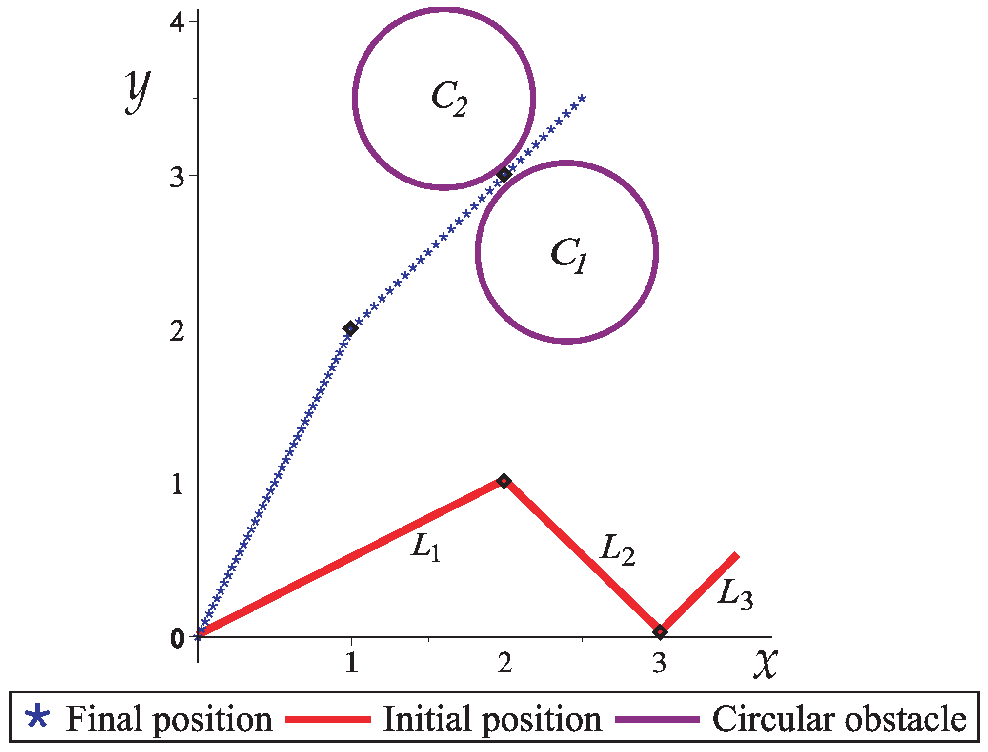
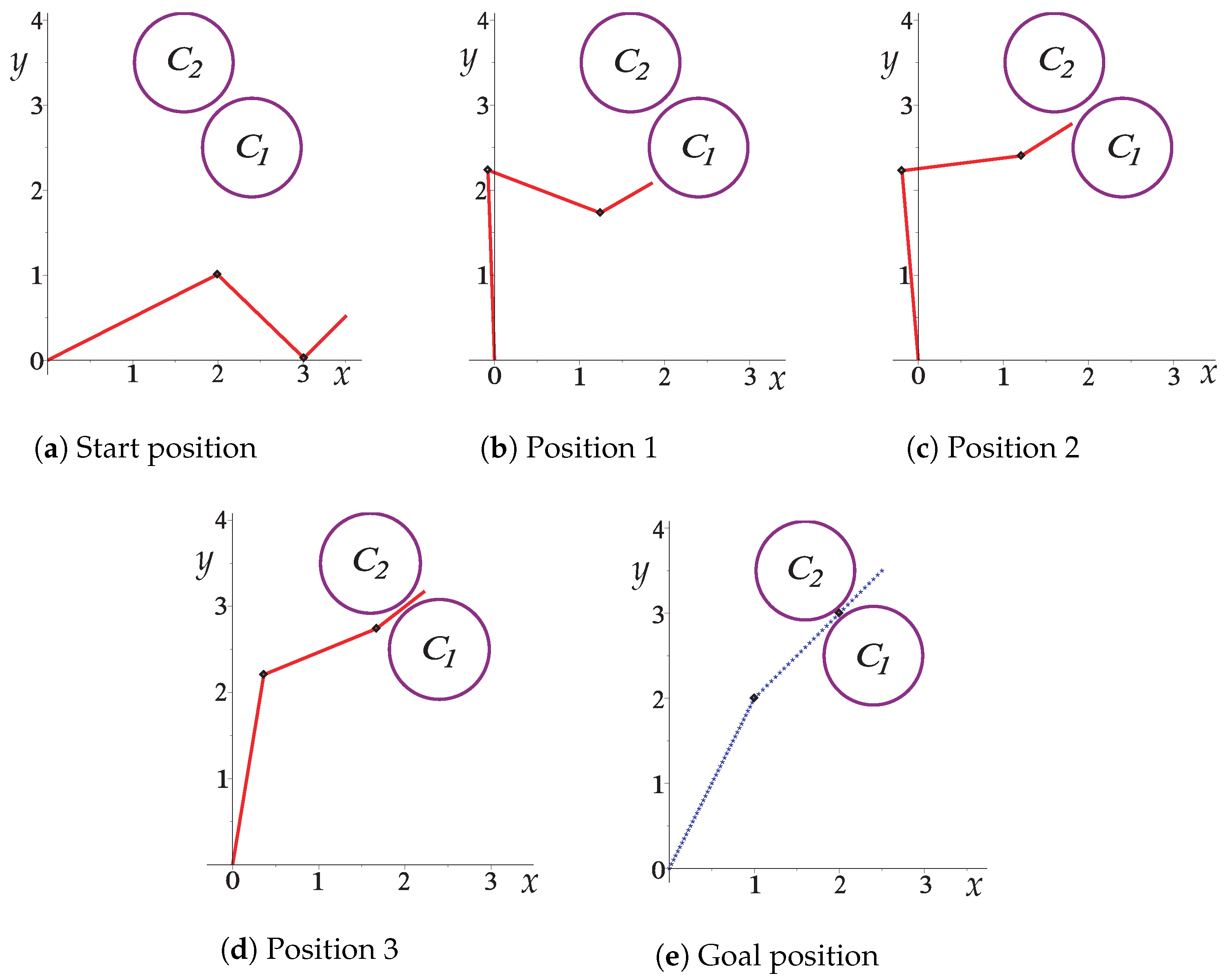
5.1. Case Study 1
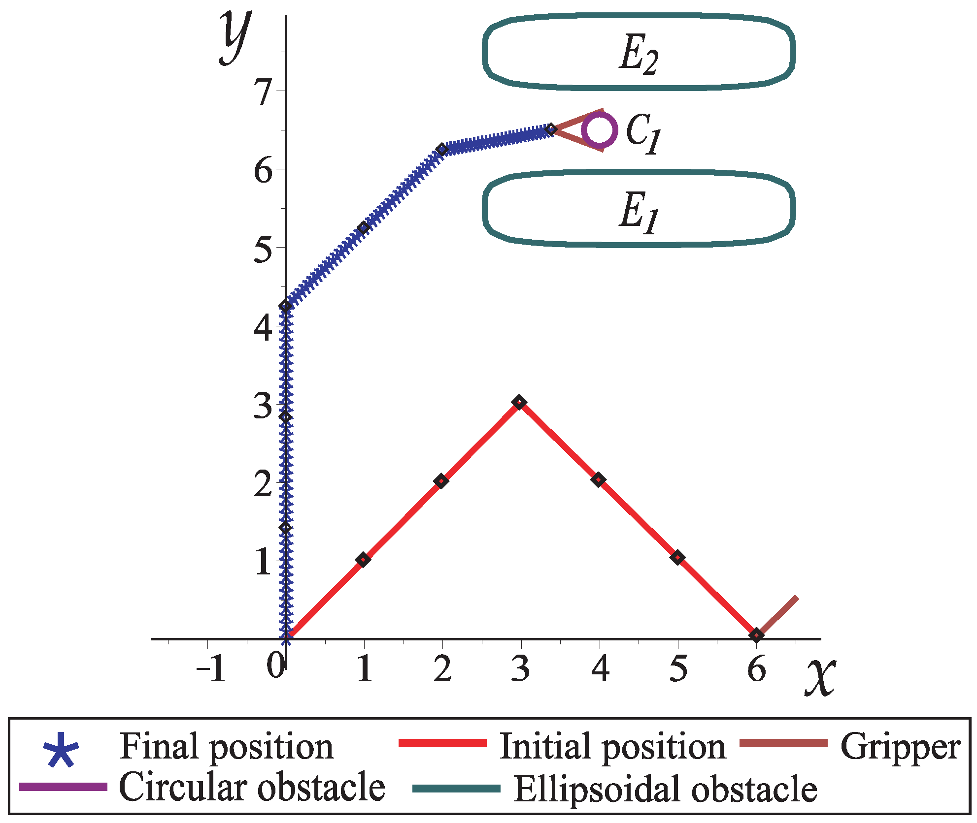
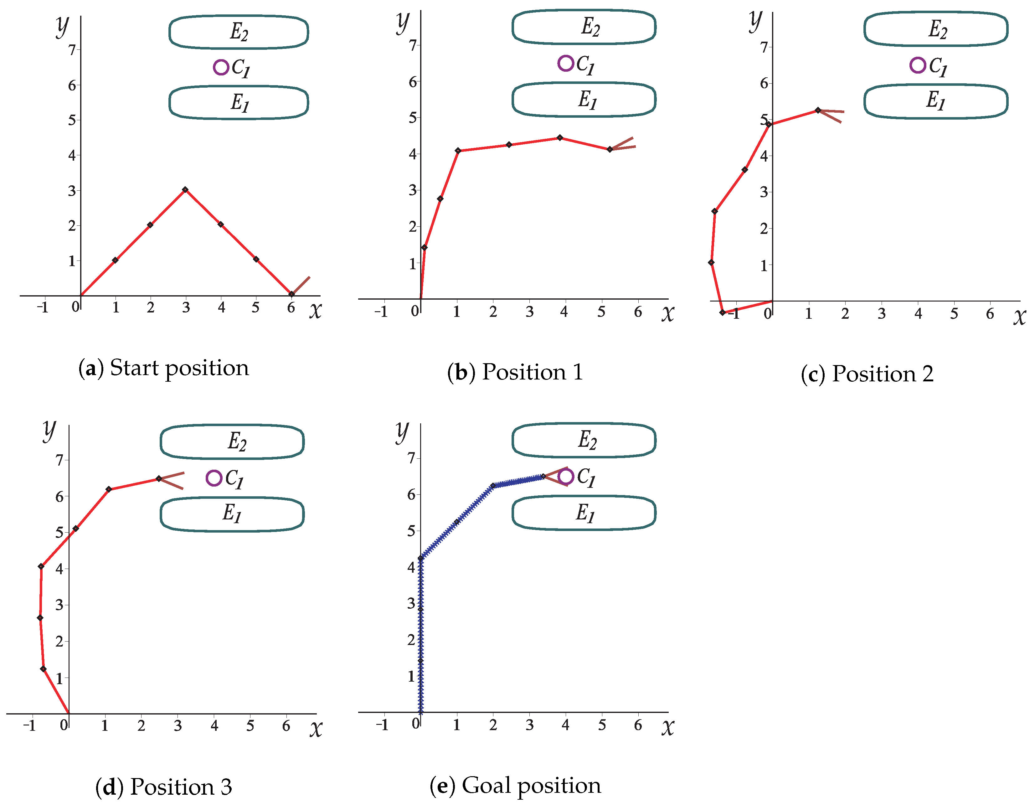
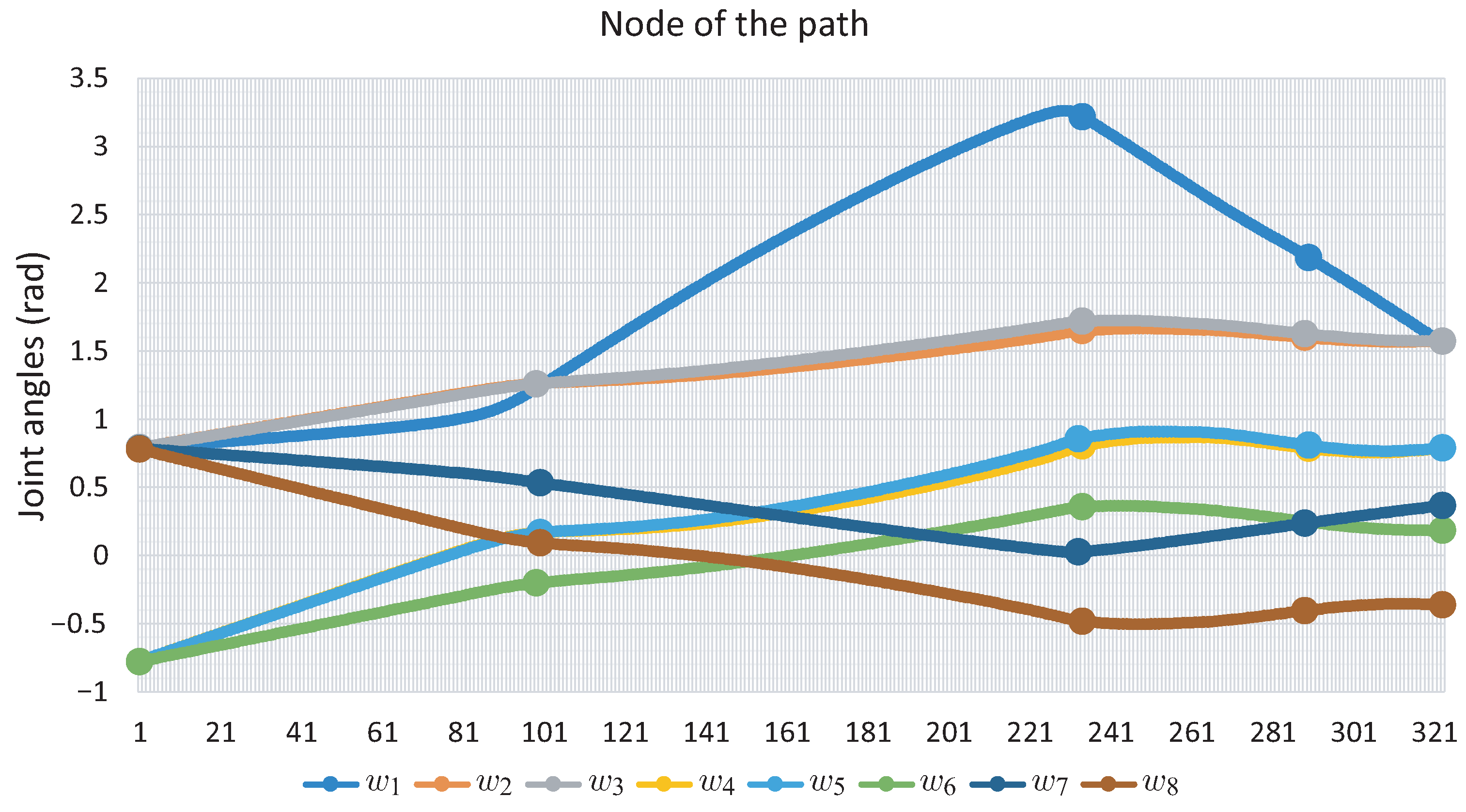
5.2. Case Study 2
5.3. Case Study 3
6. Implementation of the Proposed Method in the CRS Catalyst-5 Robot
- 1.
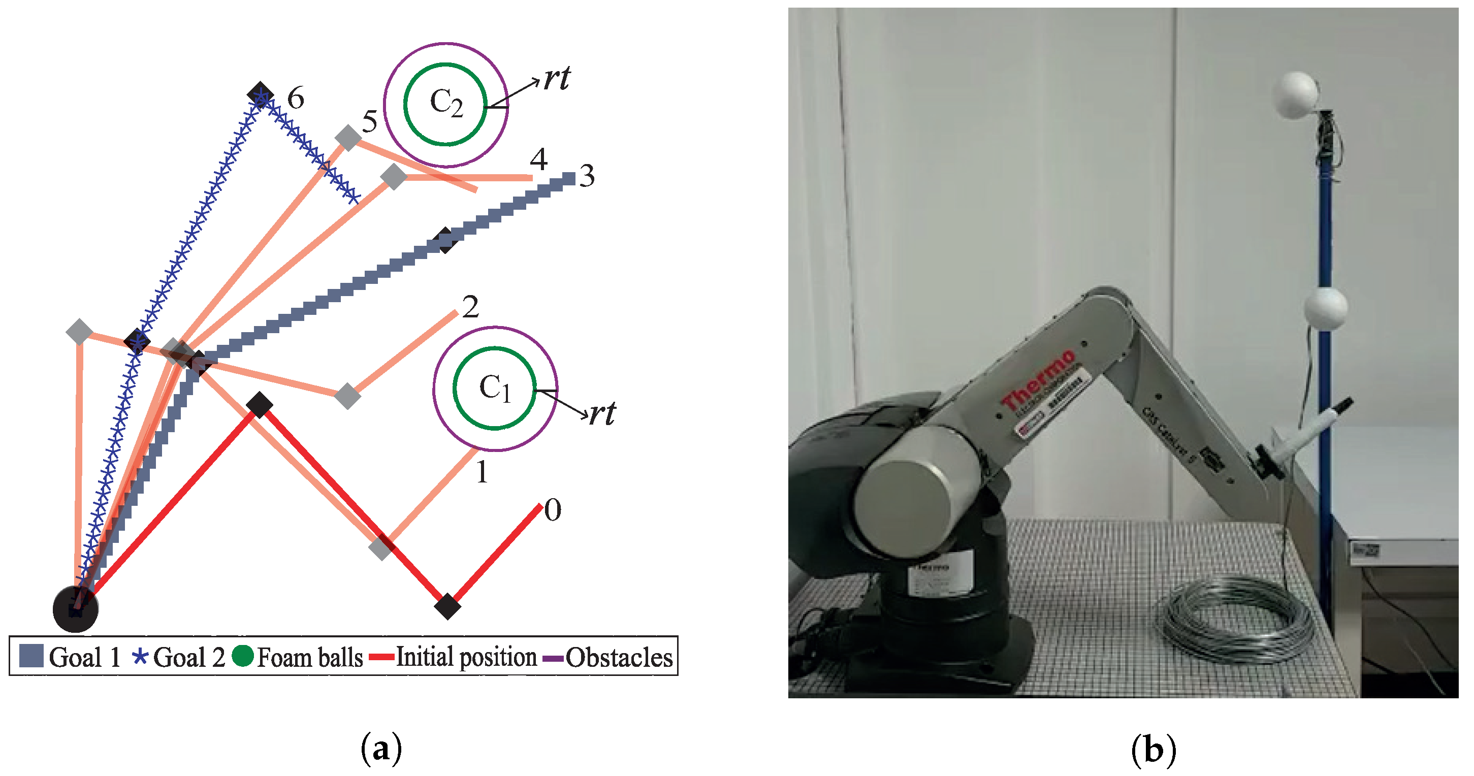
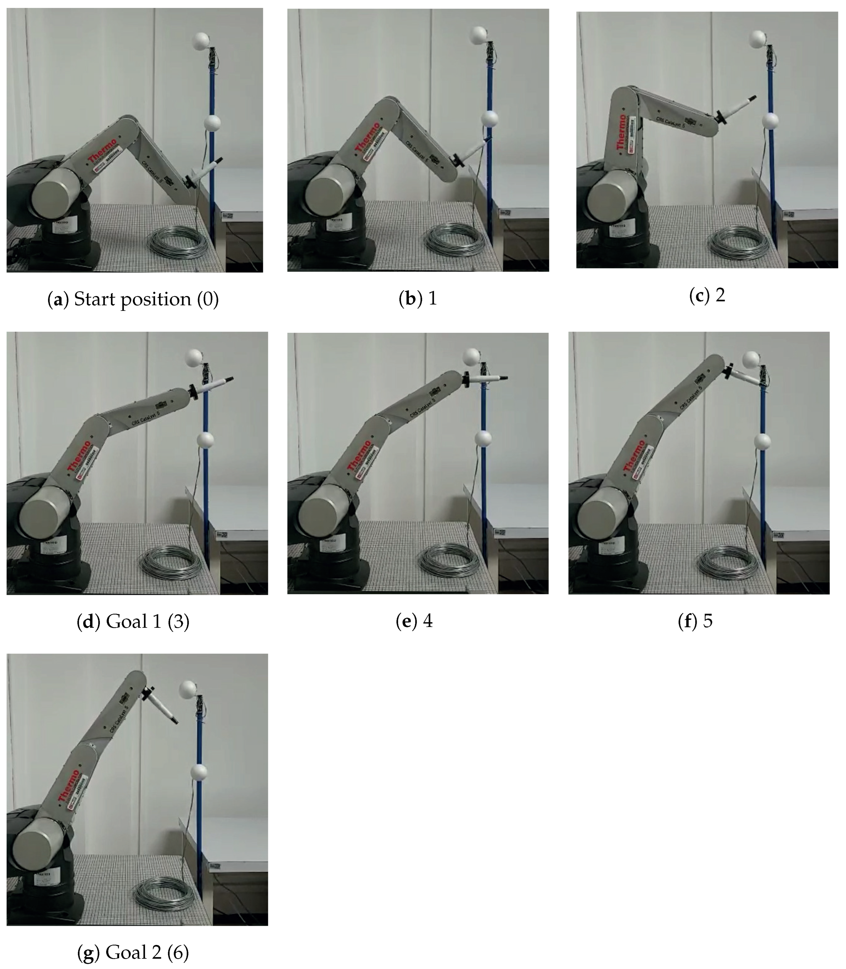
- First, the workspace to be solved was established. A three-link robot arm with normalized dimensions regarding the CRS CataLyst-5 robot was used. The circular obstacles had a tolerance radius , which guaranteed no collision of the robot arm with the obstacle (foam balls). For this case, two goals (goal1 and goal2) were set and are depicted in Figure 22 by the line formed by gray boxes and the blue line formed by asterisks, respectively. The movements of the robot arm are semi-transparent. The robot arm first reaches Goal 1 (the first homotopic path has been followed). Then, the endpoint of this path is used as the starting position to obtain the second homotopic path and reach Goal 2. In this way, a single path is obtained capable of avoiding obstacles and meeting both goals. The computation time and memory consumption were 2 milliseconds and 0.924 KB, respectively. The sequence of movements is executed by the robotic arm, as shown in Figure 22a.
- 2.
- The second stage of this process is to adjust the numeric homotopy path data to the correct instructions for the CRS CataLyst-5 arm to follow the path. The CRS-CataLyst-5 robot has five degrees of freedom, a teach pendant, and a controller for interpreting and processing the instructions sent by the computer through its Robcomm3 software to generate the movements of the robot [46,47]. Figure 22b depicts the robotic arm workspace. From Figure 23 (implementation), the sequence of movements of Figure 22a (simulation) is corroborated.
7. Conclusions and Future Work
Author Contributions
Funding
Institutional Review Board Statement
Informed Consent Statement
Data Availability Statement
Acknowledgments
Conflicts of Interest
References
- Baek, D.; Hwang, M.; Kim, H.; Kwon, D.S. Path planning for automation of surgery robot based on probabilistic roadmap and reinforcement learning. In Proceedings of the 2018 15th International Conference on Ubiquitous Robots (UR), Honolulu, HI, USA, 26–30 June 2018; pp. 342–347. [Google Scholar]
- Bauzano, E.; Estebanez, B.; Garcia-Morales, I.; Munoz, V.F. Collaborative human–robot system for hals suture procedures. IEEE Syst. J. 2014, 10, 957–966. [Google Scholar] [CrossRef]
- Roy, R.; Mahadevappa, M.; Kumar, C. Trajectory path planning of EEG controlled robotic arm using GA. Procedia Comput. Sci. 2016, 84, 147–151. [Google Scholar] [CrossRef] [Green Version]
- Kopperger, E.; List, J.; Madhira, S.; Rothfischer, F.; Lamb, D.C.; Simmel, F.C. A self-assembled nanoscale robotic arm controlled by electric fields. Science 2018, 359, 296–301. [Google Scholar] [CrossRef] [PubMed] [Green Version]
- Flores-Abad, A.; Ma, O.; Pham, K.; Ulrich, S. A review of space robotics technologies for on-orbit servicing. Prog. Aerosp. Sci. 2014, 68, 1–26. [Google Scholar] [CrossRef] [Green Version]
- Kularatne, D.; Bhattacharya, S.; Hsieh, M.A. Optimal path planning in time-varying flows using adaptive discretization. IEEE Robot. Autom. Lett. 2017, 3, 458–465. [Google Scholar] [CrossRef]
- Grushko, S.; Vysocký, A.; Oščádal, P.; Vocetka, M.; Novák, P.; Bobovský, Z. Improved Mutual Understanding for Human-Robot Collaboration: Combining Human-Aware Motion Planning with Haptic Feedback Devices for Communicating Planned Trajectory. Sensors 2021, 21, 3673. [Google Scholar] [CrossRef]
- Zhao, S.; Zhao, J.; Sui, D.; Wang, T.; Zheng, T.; Zhao, C.; Zhu, Y. Modular Robotic Limbs for Astronaut Activities Assistance. Sensors 2021, 21, 6305. [Google Scholar] [CrossRef]
- Rybus, T.; Wojtunik, M.; Basmadji, F.L. Optimal collision-free path planning of a free-floating space robot using spline-based trajectories. Acta Astronaut. 2022, 190, 395–408. [Google Scholar] [CrossRef]
- Martín Barrio, A.; Terrile, S.; Barrientos, A.; del Cerro, J. Robots Hiper-Redundantes: Clasificación, Estado del Arte y Problemática. Rev. Iberoam. Autom. Inform. Ind. 2018, 15, 351–362. [Google Scholar] [CrossRef]
- Cowan, L.S.; Walker, I.D. The importance of continuous and discrete elements in continuum robots. Int. J. Adv. Robot. Syst. 2013, 10, 165. [Google Scholar] [CrossRef]
- Lau, K.; Leung, E.; Poon, C.; Lau, J.; Yam, Y.; Chiu, P. Development of an Endoscopic Surgical Robotic System–from Bench to Animal Studies. In Proceedings of the Hamlyn Symposium on Medical Robotics, London, UK, 25–28 June 2017; p. 1. [Google Scholar]
- Berthet-Rayne, P.; Gras, G.; Leibrandt, K.; Wisanuvej, P.; Schmitz, A.; Seneci, C.A.; Yang, G.Z. The i 2 snake robotic platform for endoscopic surgery. Ann. Biomed. Eng. 2018, 46, 1663–1675. [Google Scholar] [CrossRef] [PubMed] [Green Version]
- Deng, J.; Meng, B.H.; Kanj, I.; Godage, I.S. Near-optimal Smooth Path Planning for Multisection Continuum Arms. In Proceedings of the 2019 2nd IEEE International Conference on Soft Robotics (RoboSoft), Seoul, Korea, 14–18 April 2019; pp. 416–421. [Google Scholar]
- Shiller, Z. Off-line and on-line trajectory planning. In Motion and Operation Planning of Robotic Systems; Springer: Berlin/Heidelberg, Germany, 2015; pp. 29–62. [Google Scholar]
- LaValle, S.M. Planning Algorithms; Cambridge University Press: Cambridge, UK, 2006. [Google Scholar]
- Murray, S.; Floyd-Jones, W.; Qi, Y.; Sorin, D.J.; Konidaris, G.D. Robot Motion Planning on a Chip. In Proceedings of the Robotics: Science and Systems, Ann Arbor, MI, USA, 18–22 June 2016. [Google Scholar]
- Brass, P.; Vigan, I.; Xu, N. Shortest path planning for a tethered robot. Comput. Geom. 2015, 48, 732–742. [Google Scholar] [CrossRef]
- Fu, B.; Chen, L.; Zhou, Y.; Zheng, D.; Wei, Z.; Dai, J.; Pan, H. An improved A* algorithm for the industrial robot path planning with high success rate and short length. Robot. Auton. Syst. 2018, 106, 26–37. [Google Scholar] [CrossRef]
- Baghli, F.Z.; Elbakkali, L.; Lakhal, Y. Optimization of arm manipulator trajectory planning in the presence of obstacles by ant colony algorithm. Procedia Eng. 2017, 181, 560–567. [Google Scholar] [CrossRef]
- Gai, S.N.; Sun, R.; Chen, S.J.; Ji, S. 6-DOF robotic obstacle avoidance path planning based on artificial potential field method. In Proceedings of the 2019 16th International Conference on Ubiquitous Robots (UR), Jeju, Korea, 24–27 June 2019; pp. 165–168. [Google Scholar]
- Vazquez-Leal, H.; Marin-Hernandez, A.; Khan, Y.; Yıldırım, A.; Filobello-Nino, U.; Castañeda-Sheissa, R.; Jimenez-Fernandez, V.M. Exploring collision-free path planning by using homotopy continuation methods. Appl. Math. Comput. 2013, 219, 7514–7532. [Google Scholar]
- Diaz-Arango, G.; Vázquez-Leal, H.; Hernandez-Martinez, L.; Pascual, M.T.S.; Sandoval-Hernandez, M. Homotopy path planning for terrestrial robots using spherical algorithm. IEEE Trans. Autom. Sci. Eng. 2017, 15, 567–585. [Google Scholar] [CrossRef]
- Diaz-Arango, G.; Vazquez-Leal, H.; Hernandez-Martinez, L.; Jimenez-Fernandez, V.M.; Heredia-Jimenez, A.; Ambrosio, R.C.; Huerta-Chua, J.; Cos-Cholula, D.; Hernandez-Mendez, S. Multiple-Target Homotopic Quasi-Complete path-planning method for Mobile Robot Using a Piecewise Linear Approach. Sensors 2020, 20, 3265. [Google Scholar]
- Liu, Y.R.; Huang, M.B.; Huang, H.P. Automated grasp planning and path planning for a robot hand-arm system. In Proceedings of the 2019 IEEE/SICE International Symposium on System Integration (SII), Paris, France, 14–16 January 2019; pp. 92–97. [Google Scholar]
- Kingston, Z.; Moll, M.; Kavraki, L.E. Sampling-based methods for motion planning with constraints. Annu. Rev. Control Robot. Auton. Syst. 2018, 1, 159–185. [Google Scholar] [CrossRef] [Green Version]
- Vien, N.A.; Toussaint, M. POMDP manipulation via trajectory optimization. In Proceedings of the 2015 IEEE/RSJ International Conference on Intelligent Robots and Systems (IROS), Hamburg, Germany, 28 September–2 October 2015; pp. 242–249. [Google Scholar]
- Samaniego, R.; Rodríguez, R.; Vázquez, F.; López, J. Efficient path planing for articulated vehicles in cluttered environments. Sensors 2020, 20, 6821. [Google Scholar]
- Kang, T.W.; Kang, J.G.; Jung, J.W. A Bidirectional Interpolation Method for Post-Processing in Sampling-Based Robot Path Planning. Sensors 2021, 21, 7425. [Google Scholar]
- Jeon, G.Y.; Jung, J.W. Water sink model for robot motion planning. Sensors 2019, 19, 1269. [Google Scholar] [CrossRef] [PubMed] [Green Version]
- Cao, Y.; Guo, M.; Li, Y. Obstacle-free workspace based path planning for serial manipulator. In Proceedings of the 2017 36th Chinese Control Conference (CCC), Dalian, China, 26–28 July 2017; pp. 6897–6900. [Google Scholar]
- Jena, A.; Sahu, P.K.; Bharat, S.C.; Biswal, B. Optimal trajectory planning of a 3R SCARA manipulator using geodesic. In Proceedings of the 2016 IEEE 1st International Conference on Power Electronics, Intelligent Control and Energy Systems (ICPEICES), Delhi, India, 4–6 July 2016; pp. 1–6. [Google Scholar]
- Chembuly, V.S.; Voruganti, H.K. Trajectory planning of redundant manipulators moving along constrained path and avoiding obstacles. Procedia Comput. Sci. 2018, 133, 627–634. [Google Scholar] [CrossRef]
- De Luca, A.; Oriolo, G. Trajectory planning and control for planar robots with passive last joint. Int. J. Robot. Res. 2002, 21, 575–590. [Google Scholar] [CrossRef]
- Shafiee-Ashtiani, M.; Yousefi-Koma, A.; Iravanimanesh, S.; Bashardoust, A.S. Kinematic analysis of a 3-UPU parallel Robot using the Ostrowski-Homotopy Continuation. In Proceedings of the 2016 24th Iranian Conference on Electrical Engineering (ICEE), Shiraz, Iran, 10–12 May 2016; pp. 1306–1311. [Google Scholar]
- Nor, H.M.; Rahman, A.; Ismail, A.I.M.; Majid, A.A. Super Ostrowski homotopy continuation method for solving polynomial system of equations. MATEMATIKA Malays. J. Ind. Appl. Math. 2016, 32, 53–67. [Google Scholar]
- Jiménez-Islas, H.; Martínez-González, G.M.; Navarrete-Bolaños, J.L.; Botello-Álvarez, J.E.; Oliveros-Munoz, J.M. Nonlinear homotopic continuation methods: A chemical engineering perspective review. Ind. Eng. Chem. Res. 2013, 52, 14729–14742. [Google Scholar] [CrossRef]
- Dong, B.; Yu, B.; Yu, Y. A homotopy method for finding all solutions of a multiparameter eigenvalue problem. SIAM J. Matrix Anal. Appl. 2016, 37, 550–571. [Google Scholar] [CrossRef]
- Jiménez-Islas, H.; Calderón-Ramírez, M.; Martínez-González, G.M.; Calderón-Álvarado, M.P.; Oliveros-Muñoz, J.M. Multiple solutions for steady differential equations via hyperspherical path-tracking of homotopy curves. Comput. Math. Appl. 2020, 79, 2216–2239. [Google Scholar] [CrossRef]
- Mirmohammad, S.H.; Yousefi-Koma, A.; Mohtasebi, S.S. Direct kinematics of a three revolute-prismatic-spherical parallel robot using a fast homotopy continuation method. In Proceedings of the 2016 4th International Conference on Robotics and Mechatronics (ICROM), Tehran, Iran, 26–28 October 2016; pp. 410–415. [Google Scholar]
- Gregoire, J.; Čáp, M.; Frazzoli, E. Locally optimal multi-robot navigation under delaying disturbances using homotopy constraints. Auton. Robot. 2018, 42, 895–907. [Google Scholar] [CrossRef] [Green Version]
- Vázquez-Leal, H.; Castañeda-Sheissa, R.; Rabago-Bernal, F.; Hernández-Martínez, L.; Sarmiento-Reyes, A.; Filobello-Niño, U. Powering multiparameter homotopy-based simulation with a fast path-following technique. ISRN Appl. Math. 2011, 2011, 610637. [Google Scholar] [CrossRef] [Green Version]
- Velez-Lopez, G.C.; Hernández-Martínez, L.; Diaz-Arango, G.; Vazquez-Leal, H. A Tool to Solve Nonlinear Algebraic Equations Systems. In Proceedings of the 2019 16th International Conference on Electrical Engineering, Computing Science and Automatic Control (CCE), Mexico City, Mexico, 11–13 September 2019; pp. 1–4. [Google Scholar]
- Giorgio, I.; Del Vescovo, D. Non-linear lumped-parameter modeling of planar multi-link manipulators with highly flexible arms. Robotics 2018, 7, 60. [Google Scholar] [CrossRef] [Green Version]
- Cianchetti, M.; Laschi, C.; Menciassi, A.; Dario, P. Biomedical applications of soft robotics. Nat. Rev. Mater. 2018, 3, 143–153. [Google Scholar] [CrossRef]
- CRS Robotics Corporation (Thermo CRS Limited). A255 Robot Arm User Guide For Use with C500C Controller; CRS Robotics Corporation: Burlington, ON, Canada, 2000. [Google Scholar]
- Rios, E.M.L. Prácticas Didácticas del Laboratorio de Procesos Automatizados e Integrados por Computadora (LPAIC); Instituto Politecnico Nacional: Mexico City, Mexico, 2010. [Google Scholar]
- Torres-Muñoz, D.; Hernandez-Martinez, L.; Vazquez-Leal, H. Spherical continuation algorithm with spheres of variable radius to trace homotopy curves. Int. J. Appl. Comput. Math. 2016, 2, 421–433. [Google Scholar] [CrossRef] [Green Version]
- Vazquez-Leal, H.; Jimenez-Fernandez, V.; Benhammouda, B.; Filobello-Nino, U.; Sarmiento-Reyes, A.; Ramirez-Pinero, A.; Marin-Hernandez, A.; Huerta-Chua, J. Modified hyperspheres algorithm to trace homotopy curves of non-linear circuits composed by piecewise linear modelled devices. Sci. World J. 2014, 2014, 938598. [Google Scholar] [CrossRef] [PubMed]


| Obstacle | Type of Obstacle | P | |||
|---|---|---|---|---|---|
| Circular | 2.4 | 2.5 | 0.58 | ||
| Circular | 1.6 | 3.5 | 0.58 | 0.1 | |
| Link length | , , | ||||
| Constants of auxiliary equations | , , | ||||
| Initial state of the robot arm links | , | ||||
| Final state of the robot arm links | , | ||||
| Obstacle | Type of Obstacle | P | |||||
|---|---|---|---|---|---|---|---|
| Circular | 4.0 | 6.5 | 0.2 | - | - | ||
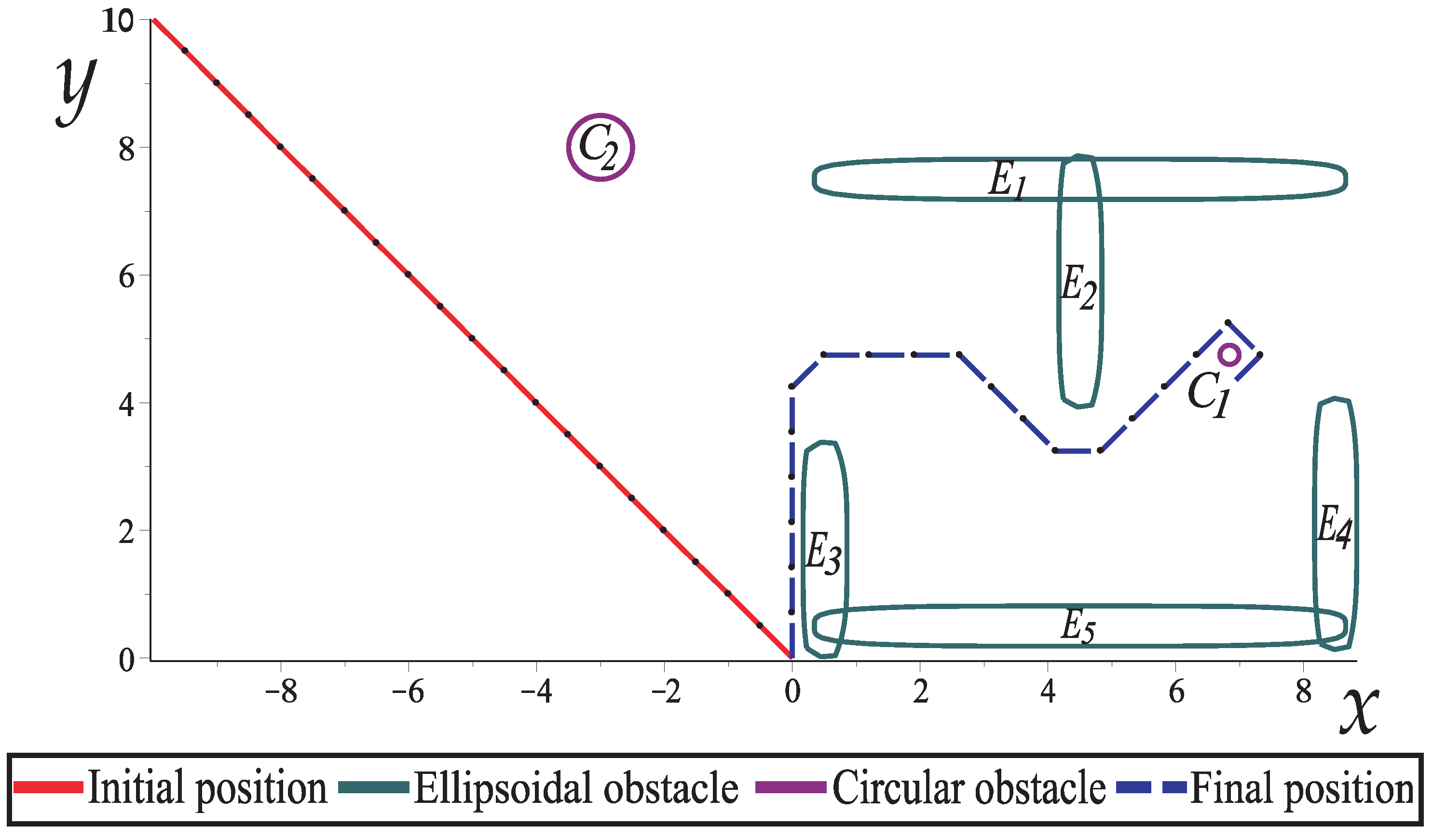
| Ellipsoid | 4.5 | 5.5 | - | 15.0 | 0.05 | ||
| Ellipsoid | 4.5 | 7.5 | - | 15.0 | 0.05 | 0.8 | |
| Link length | , | ||||||
| Constants of auxiliary equations | , , , , , , , | ||||||
| Initial state of the robot arm links | , , , , , , , | ||||||
| Final state of the robot arm links | , , , , , , , | ||||||
| Obstacle | Type of Obstacle | P | |||||
|---|---|---|---|---|---|---|---|
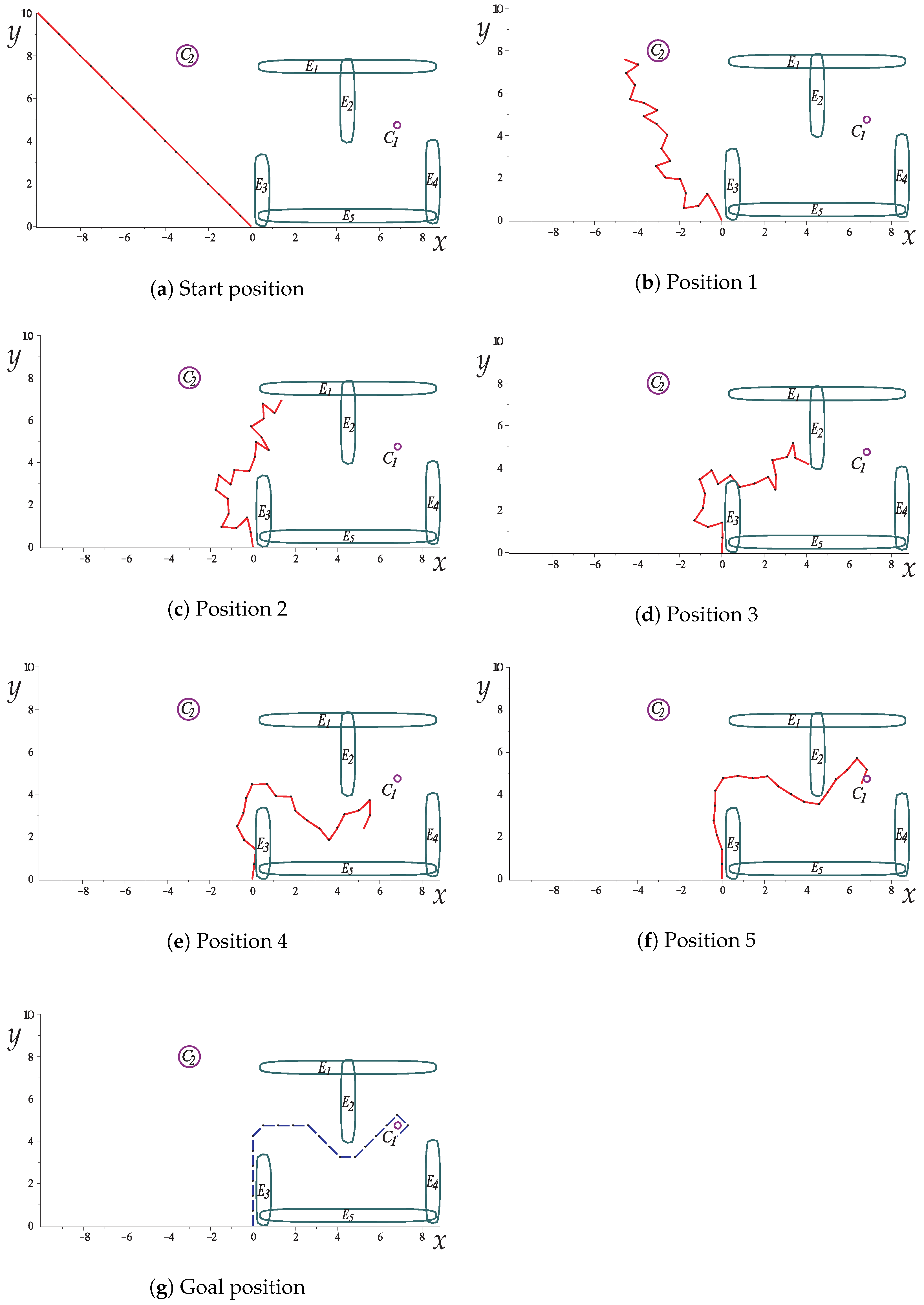
| Circular | 6.84 | 4.75 | 0.15 | - | - | 0.0000001 | |
| Circular | 8.0 | 0.5 | - | - | |||
| Ellipsoid | 4.5 | 7.5 | - | 300.0 | 0.01 | 450.0 | |
| Ellipsoid | 4.5 | 5.9 | - | 0.02 | 15.0 | 60.0 | |
| Ellipsoid | 8.5 | 2.1 | - | 0.02 | 15.0 | ||
| Ellipsoid | 4.5 | 0.5 | - | 300.0 | 0.01 | 10.0 | |
| Ellipsoid | 0.5 | 1.7 | - | 0.02 | 8.0 | ||
| Link length | |||||||
| Constants of auxiliary equations | , , , . . ., , , | ||||||
| Initial state of the robot arm links | , , , , , , , , , , , , , , , , , , , | ||||||
| Final state of the robot arm links | , , , , , , , , , , , , , , , , , , , | ||||||
| Study Case | Time | Memory | Hyperspheres | Hypersphere Radius | Number of Links | Circular Obstacle | Ellipsoid Obstacle |
|---|---|---|---|---|---|---|---|
| 1 | 3.3 ms | 1.404 KB | 146 | 0.02 | 3 | 2 | - |
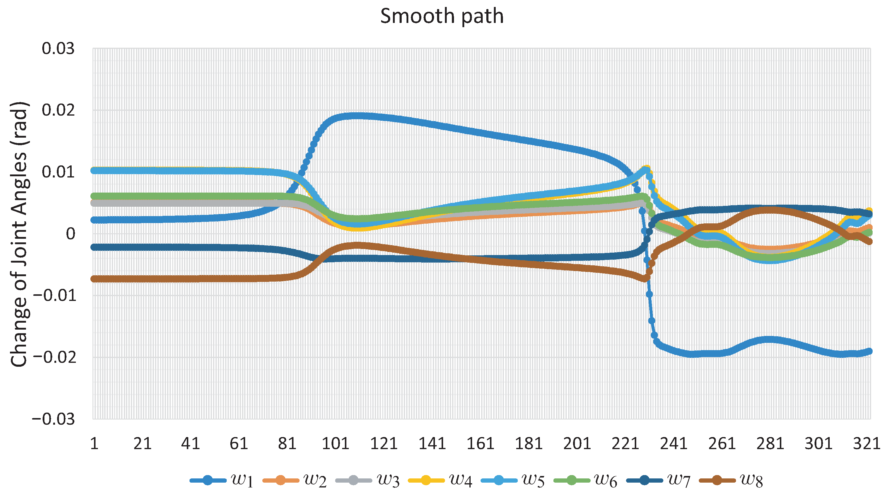
| 2 | 61.1 ms | 4.308 KB | 323 | 0.02 | 8 | 1 | 2 |
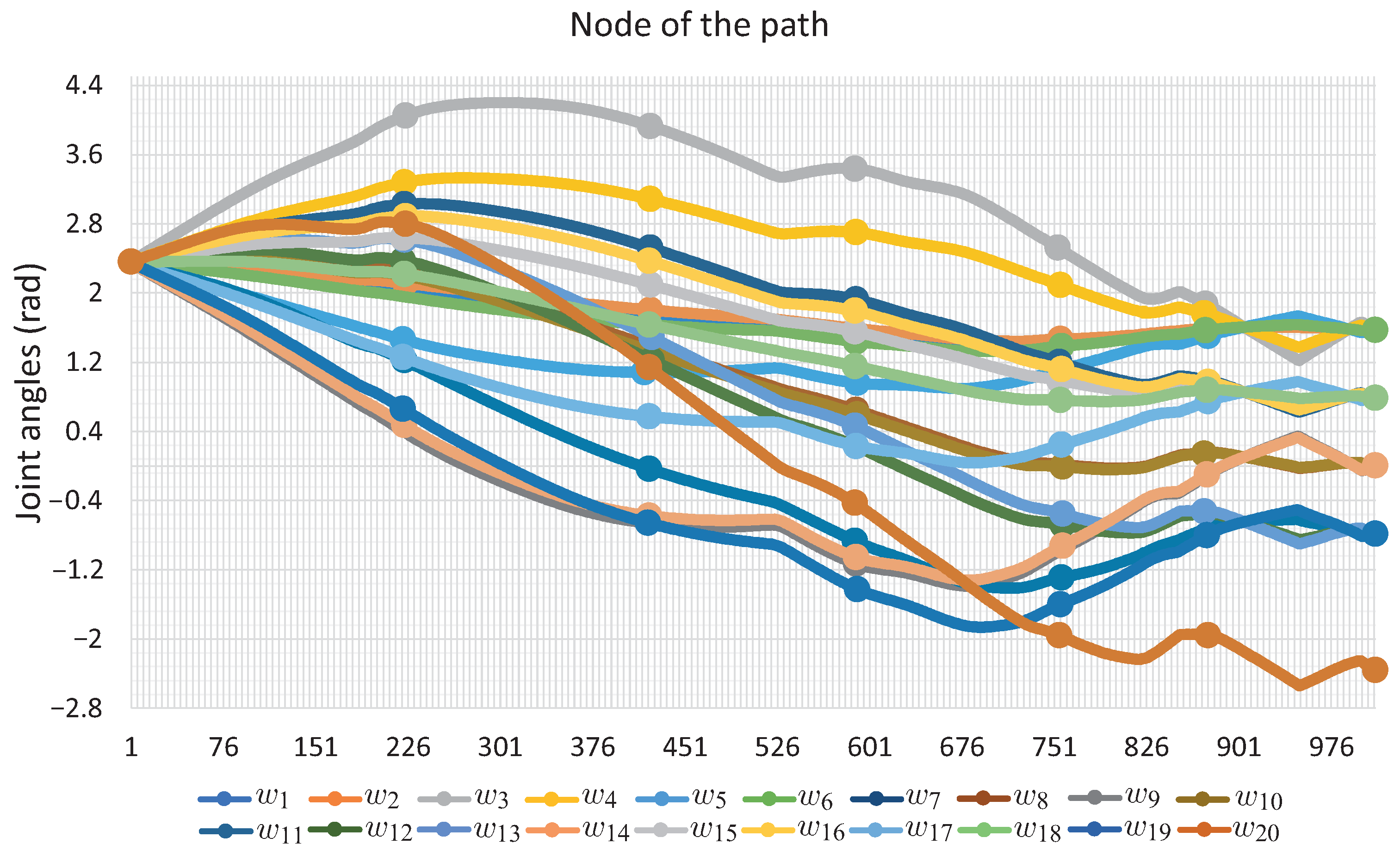
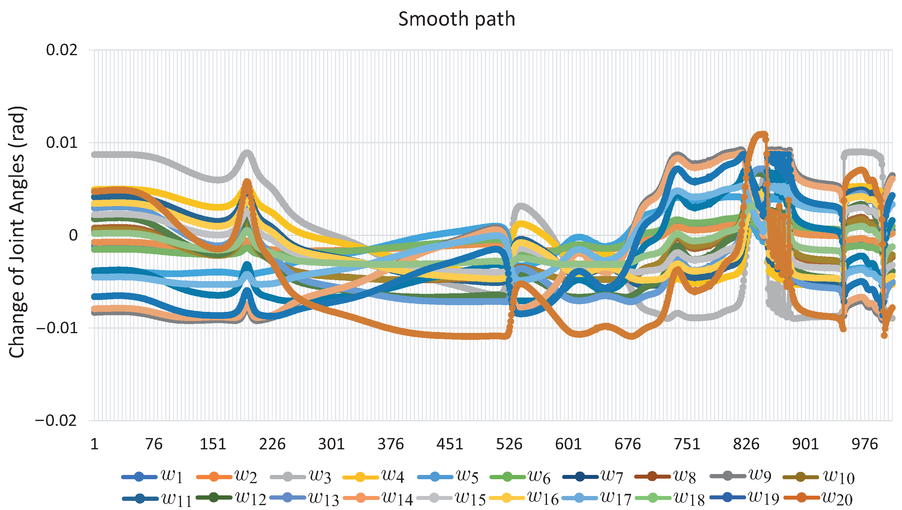
| 3 | 2.71 s | 18.272 KB | 1012 | 0.02 | 20 | 2 | 5 |
Publisher’s Note: MDPI stays neutral with regard to jurisdictional claims in published maps and institutional affiliations. |
© 2022 by the authors. Licensee MDPI, Basel, Switzerland. This article is an open access article distributed under the terms and conditions of the Creative Commons Attribution (CC BY) license (https://creativecommons.org/licenses/by/4.0/).
Share and Cite
Velez-Lopez, G.C.; Vazquez-Leal, H.; Hernandez-Martinez, L.; Sarmiento-Reyes, A.; Diaz-Arango, G.; Huerta-Chua, J.; Rico-Aniles, H.D.; Jimenez-Fernandez, V.M. A Novel Collision-Free Homotopy Path Planning for Planar Robotic Arms. Sensors 2022, 22, 4022. https://doi.org/10.3390/s22114022
Velez-Lopez GC, Vazquez-Leal H, Hernandez-Martinez L, Sarmiento-Reyes A, Diaz-Arango G, Huerta-Chua J, Rico-Aniles HD, Jimenez-Fernandez VM. A Novel Collision-Free Homotopy Path Planning for Planar Robotic Arms. Sensors. 2022; 22(11):4022. https://doi.org/10.3390/s22114022
Chicago/Turabian StyleVelez-Lopez, Gerardo C., Hector Vazquez-Leal, Luis Hernandez-Martinez, Arturo Sarmiento-Reyes, Gerardo Diaz-Arango, Jesus Huerta-Chua, Hector D. Rico-Aniles, and Victor M. Jimenez-Fernandez. 2022. "A Novel Collision-Free Homotopy Path Planning for Planar Robotic Arms" Sensors 22, no. 11: 4022. https://doi.org/10.3390/s22114022