
Development of an Electronic Stethoscope and a Classification Algorithm for Cardiopulmonary Sounds †

 , and
, and
Abstract
:1. Introduction
2. Materials and Methods
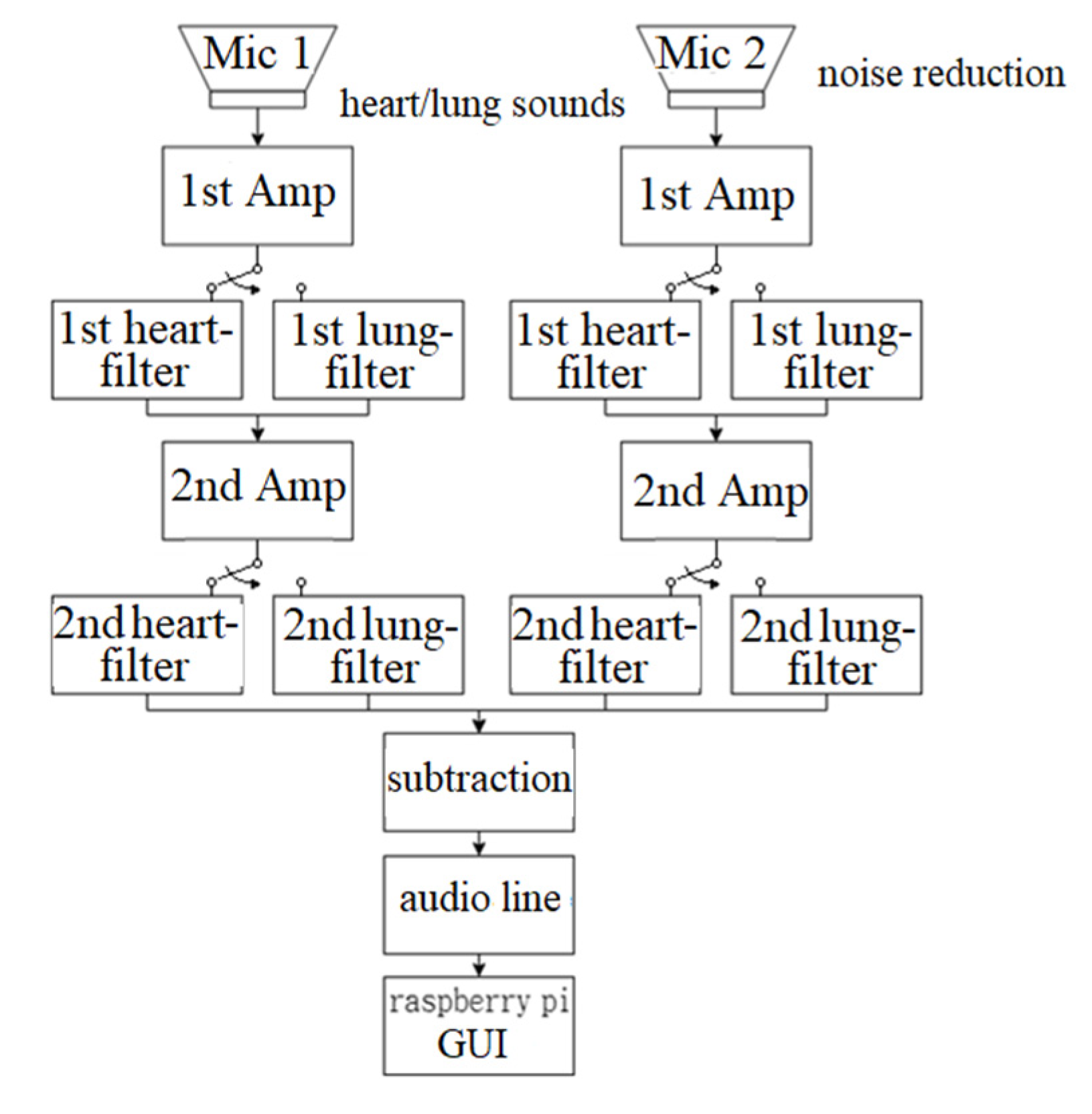
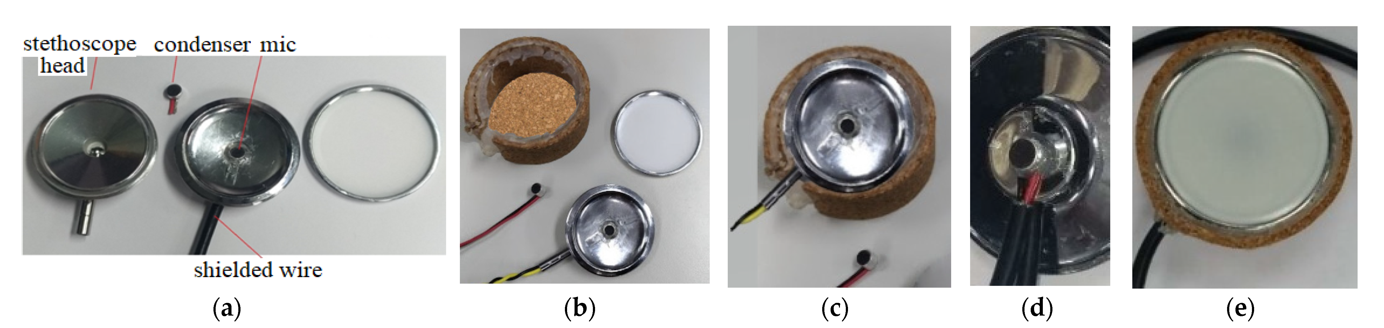
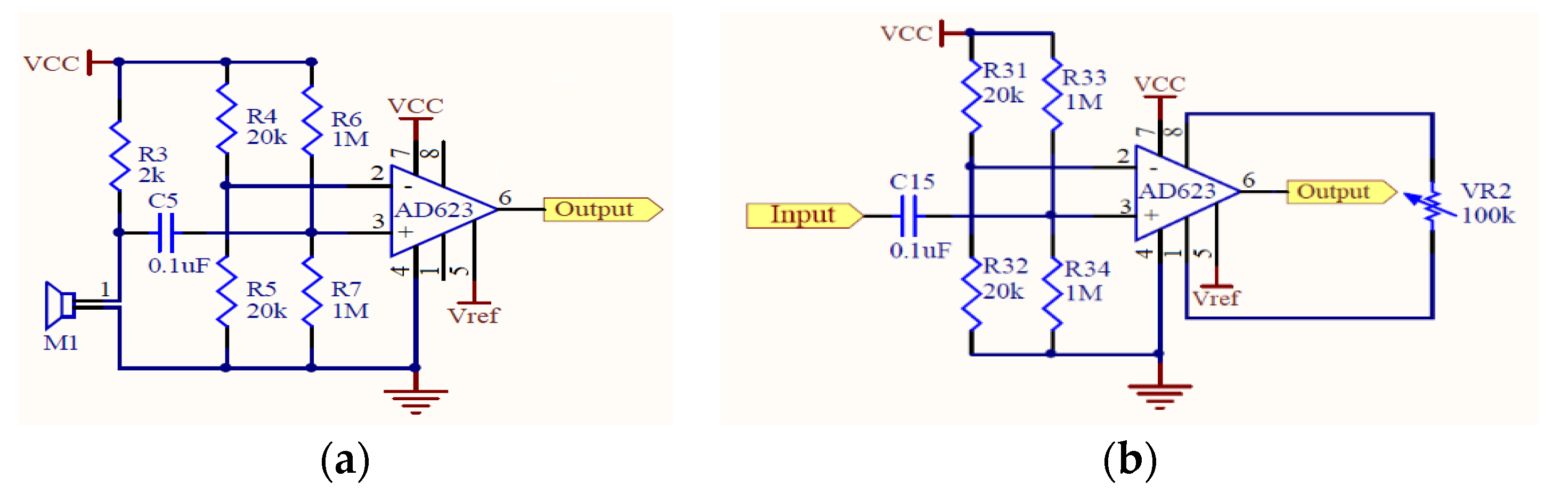
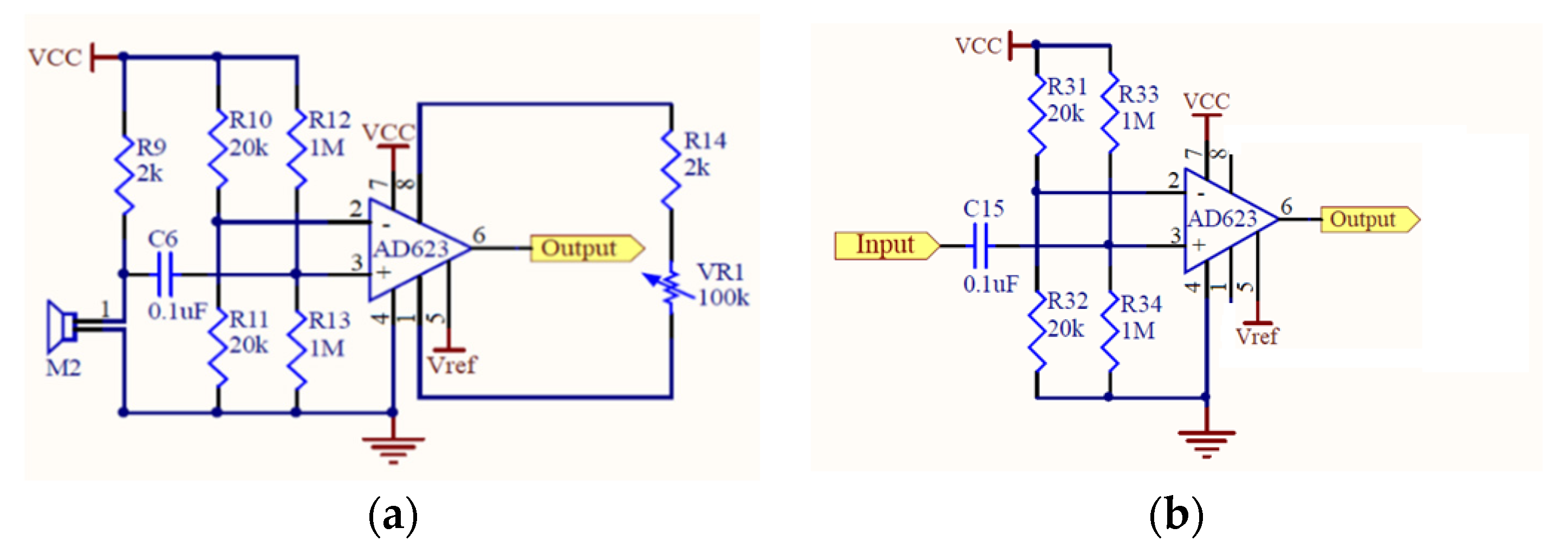
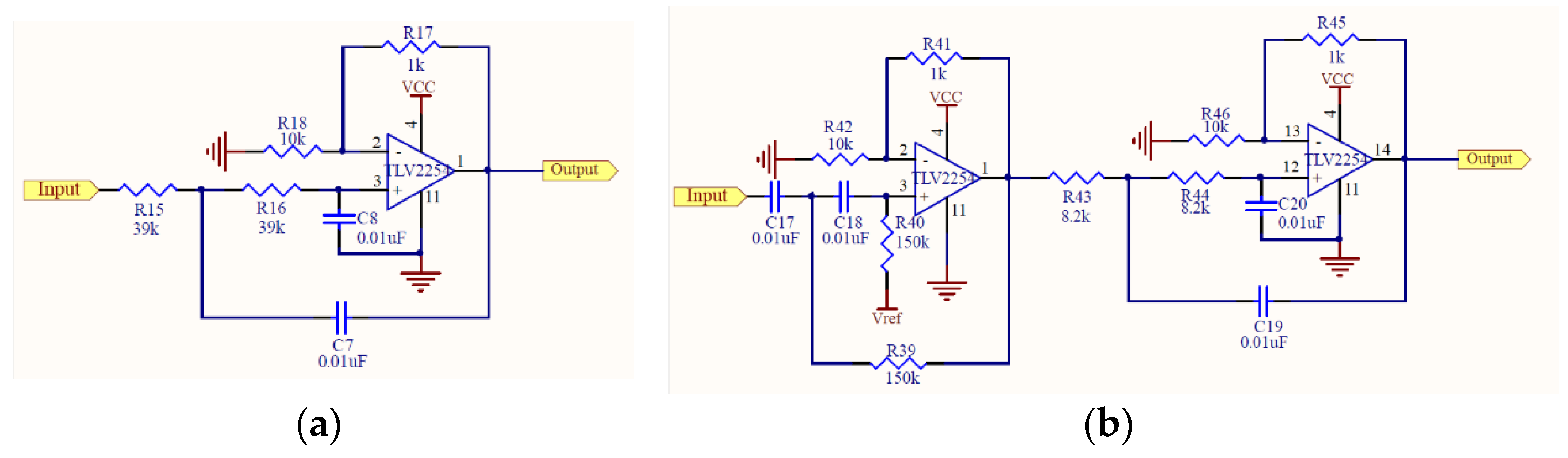
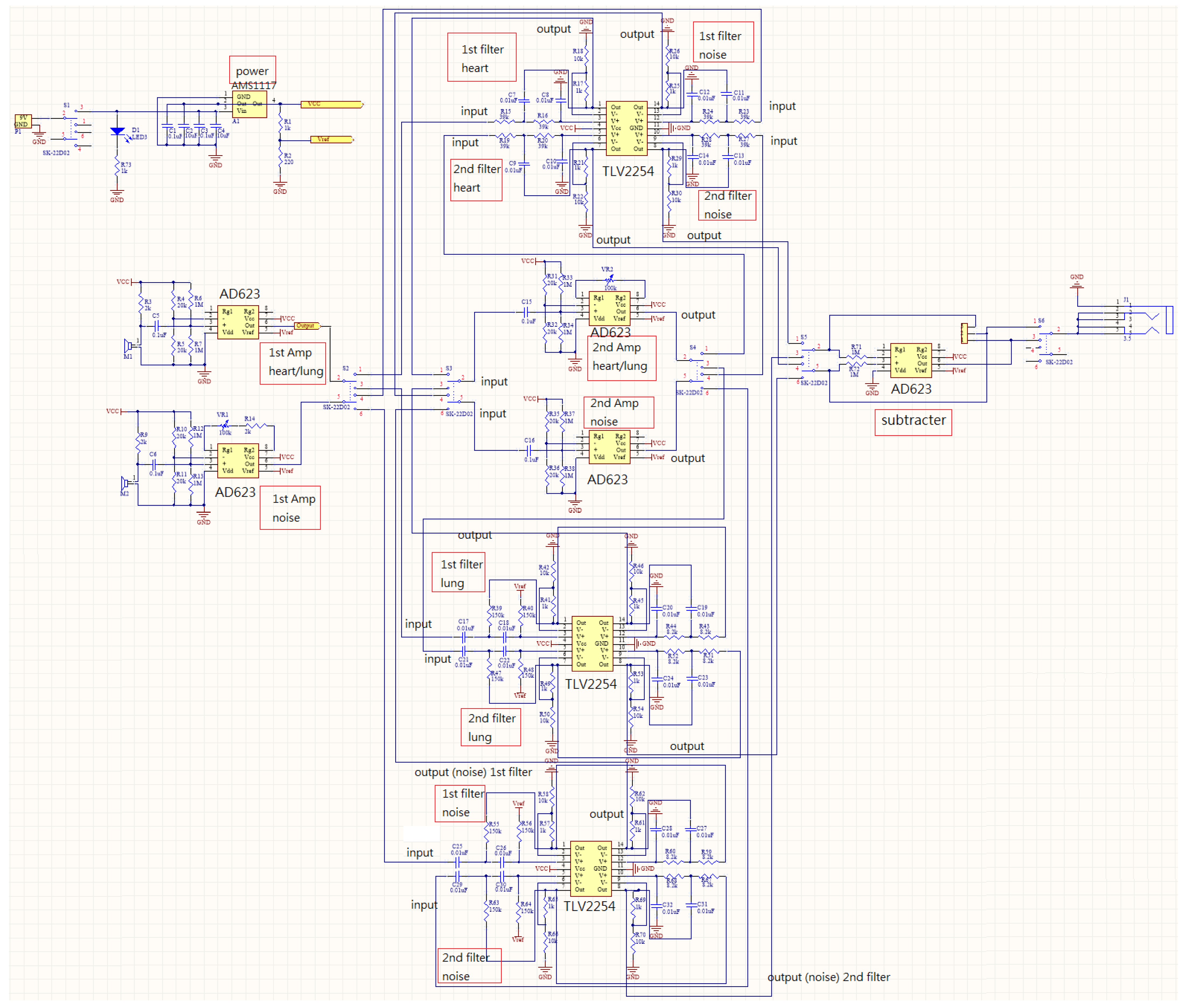
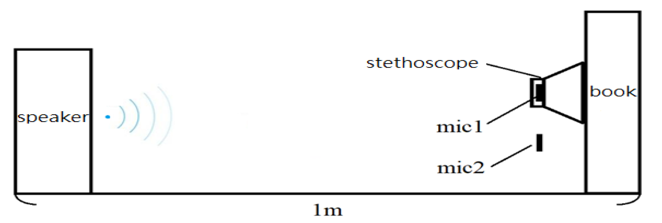
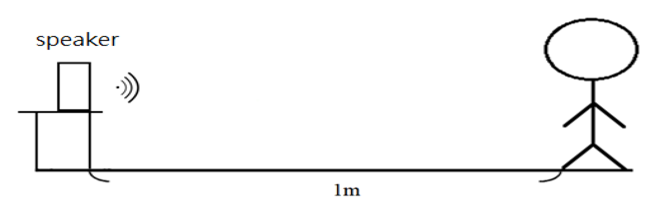
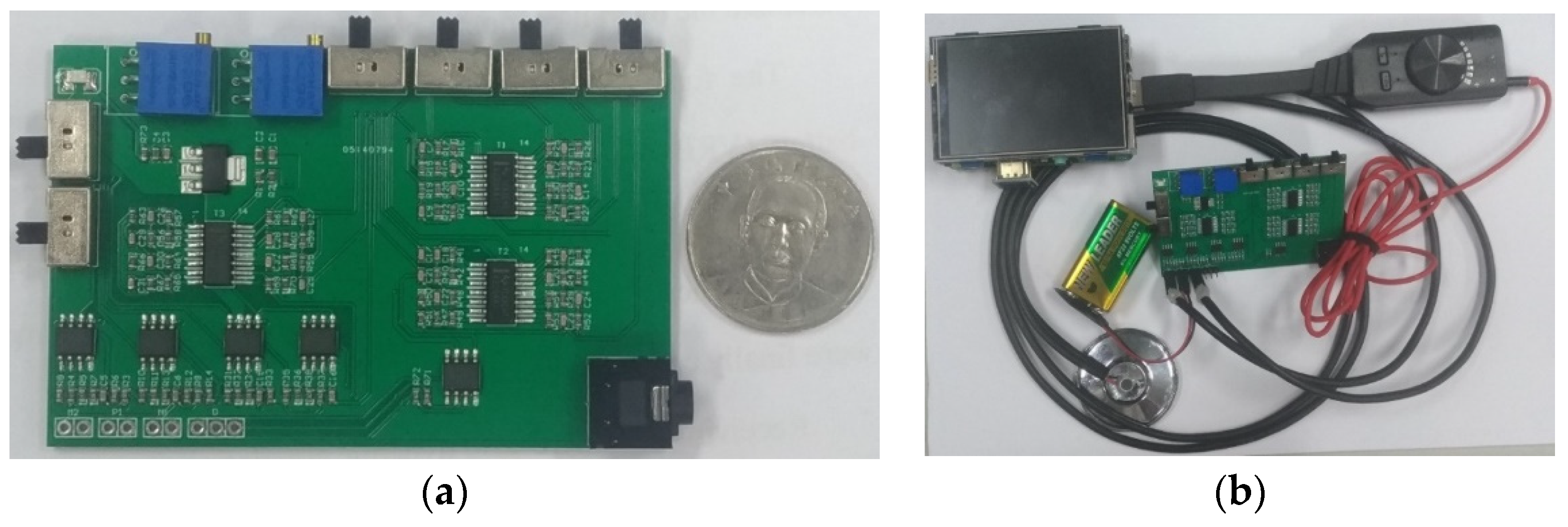
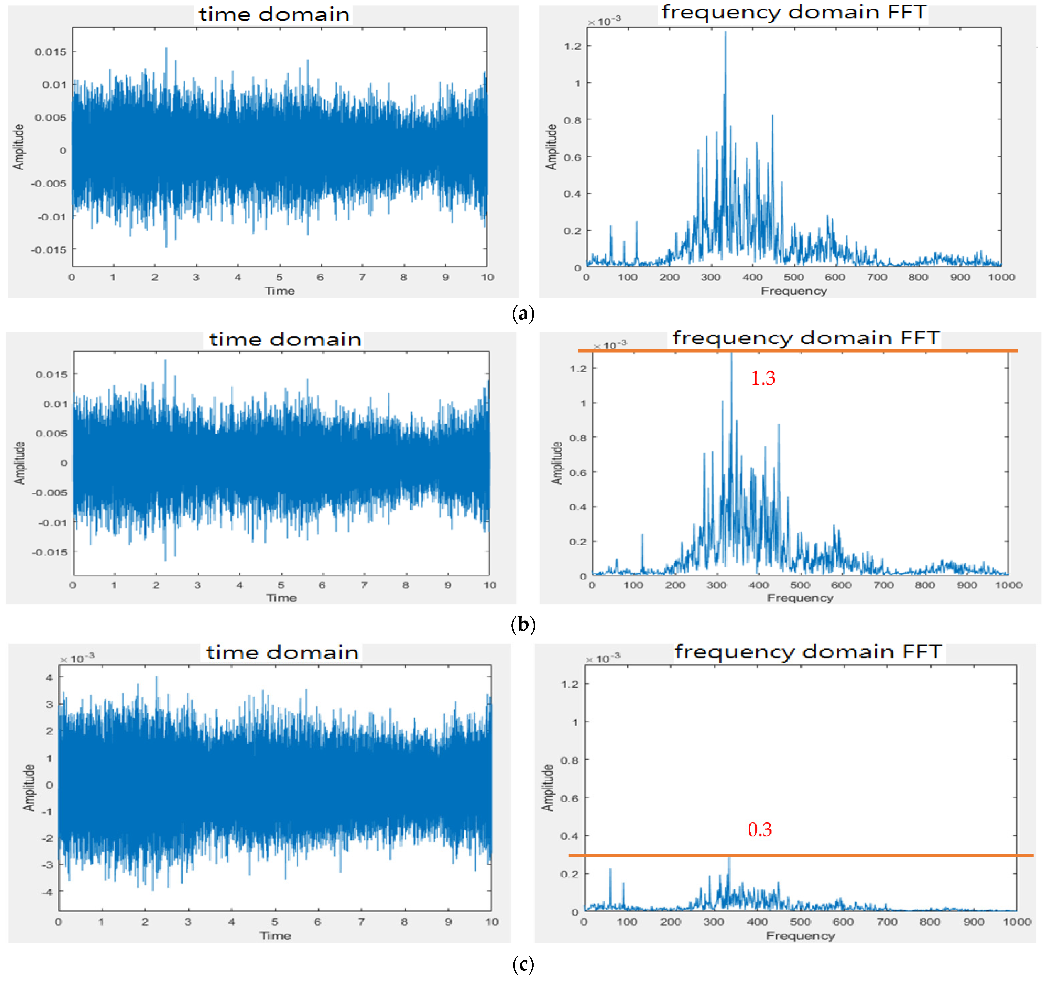
2.1. Design of Electronic Stethoscope
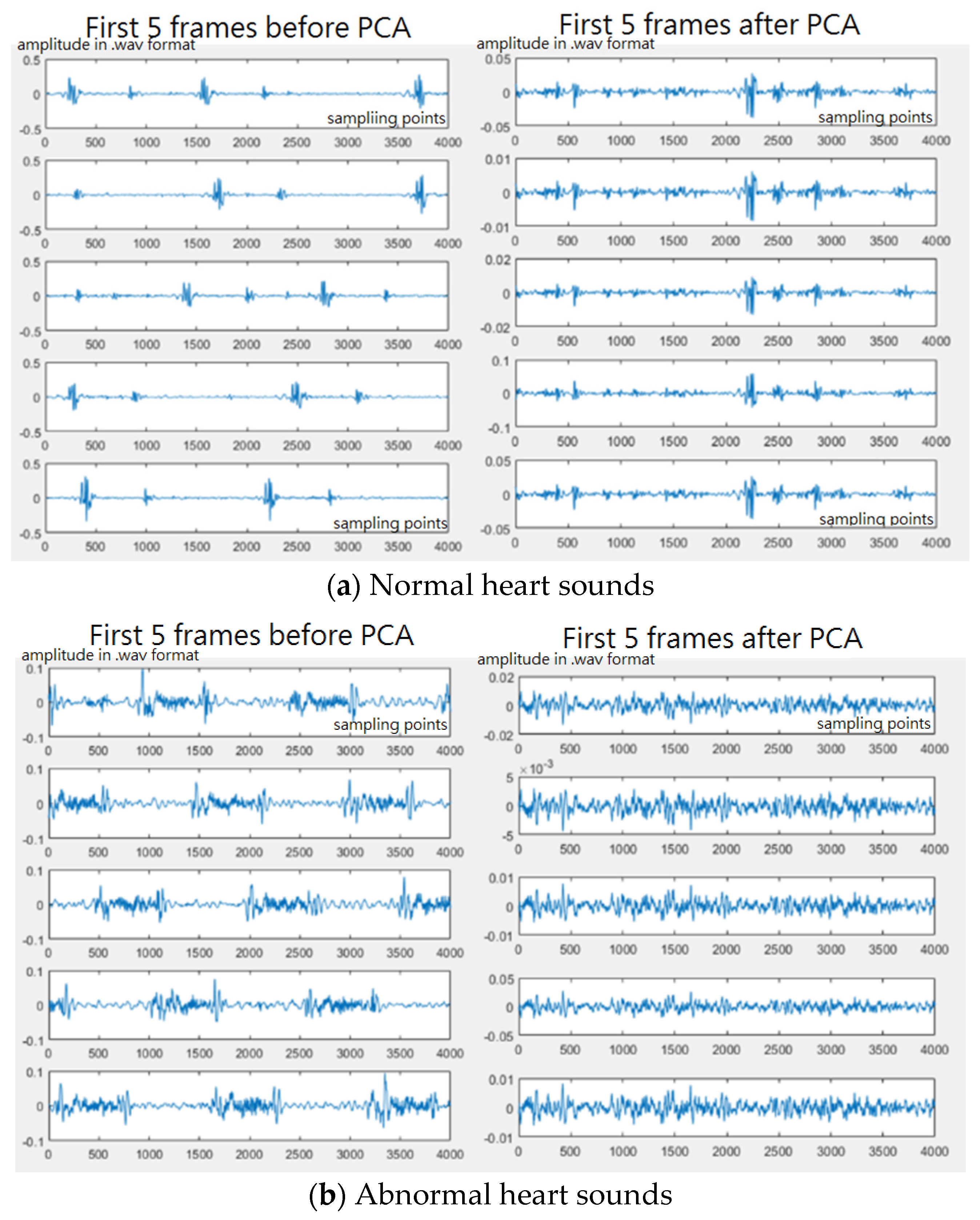
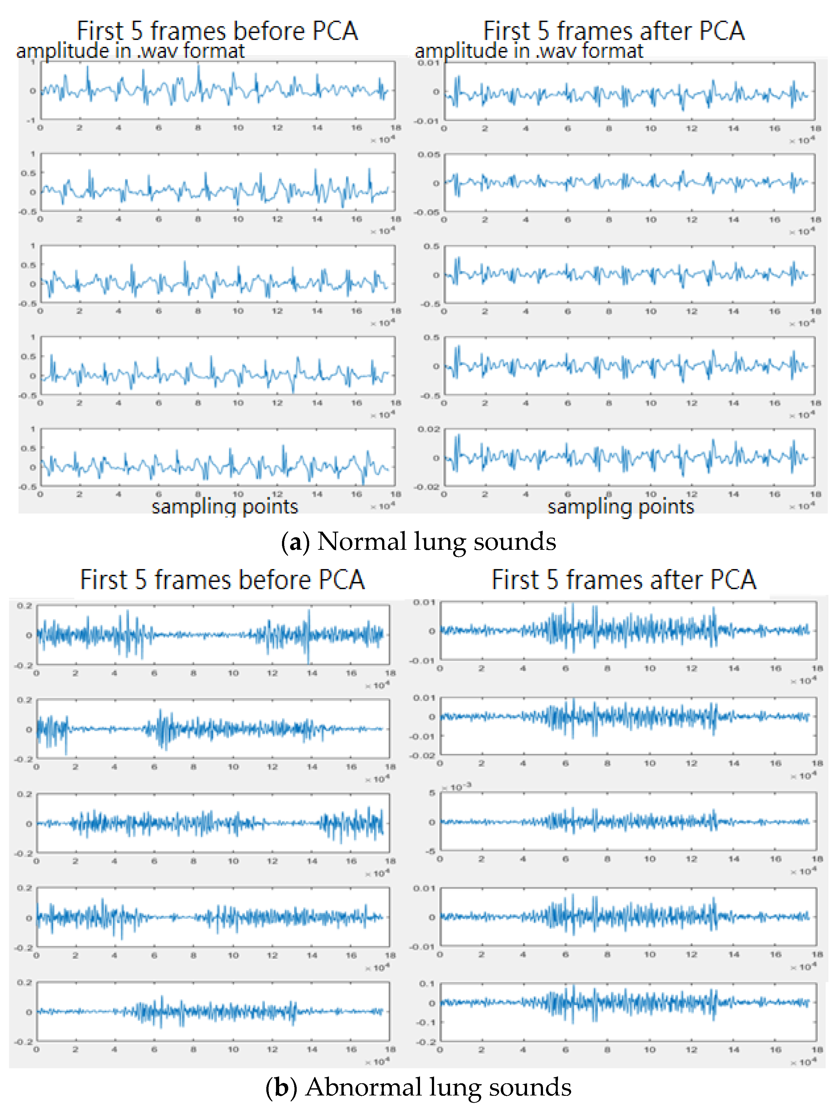
2.2. Heart/Lung Sound Classification
2.2.1. Pre-Processing
2.2.2. Feature Extraction
2.2.3. Classifier
3. Results
3.1. Design of Electronic Stethoscope
3.2. Heart/Lung Sound Classification
4. Discussion
4.1. Design of Electronic Stethoscope
4.2. Heart/Lung Sound Classification
5. Conclusions
Author Contributions
Funding
Institutional Review Board Statement
Informed Consent Statement
Data Availability Statement
Conflicts of Interest
References
- McLane, I.; Emmanouilidou, D.; West, J.E.; Elhilali, M. Design and Comparative Performance of a Robust Lung Auscultation System for Noisy Clinical Settings. IEEE J. Biomed. Health Inform. 2021, 25, 2583–2594. [Google Scholar] [CrossRef] [PubMed]
- Zhang, X.; Maddipatla, D.; Narakathu, B.B.; Bazuin, B.J.; Atashbar, M.Z. Development of a Novel Wireless Multi-Channel Stethograph System for Monitoring Cardiovasculara and Cardiopulmonary Diseasses. IEEE Access 2021, 9, 128951–128964. [Google Scholar] [CrossRef]
- Toda, M.; Thompson, M.L. Contact-type Vibration Sensors Using Curved Clamped PVDF Film. IEEE Sens. J. 2006, 6, 1170–1177. [Google Scholar] [CrossRef]
- Duan, S.; Wang, W.; Zhang, S.; Yang, X.; Zhang, Y.; Zhang, G. A Bionic MEMS Electronic Stethoscope with Double-Sided Diaphragm Packaging. IEEE Access 2021, 9, 27122–27129. [Google Scholar] [CrossRef]
- Shi, P.; Li, Y.; Zhang, W.; Zhang, G.; Cui, J.; Wang, S.; Wang, B. Design and Implementation of Bionic MEMS Electronic Heart Sound Stethoscope. IEEE Sens. J. 2022, 22, 1163–1172. [Google Scholar] [CrossRef]
- Andreozzi, E.; Fratini, A.; Esposito, D.; Naik, G.; Polley, C.; Gargiulo, G.D.; Bifulco, P. Forcecardiography: A Novel Technique to Measure Heart Mechanical Vibrations onto the Chest Wall. Sensors 2020, 20, 3885. [Google Scholar] [CrossRef] [PubMed]
- Andreozzi, E.; Gargiulo, G.D.; Esposito, D.; Bifulco, P. A Novel Broadband Forcecardiography Sensor for Simultaneous Monitoring of Respiration, Infrasonic Cardiac Vibrations and Heart Sounds. Front. Physiol. 2021, 18, 725716. [Google Scholar] [CrossRef] [PubMed]
- Chien, J.; Huang, M.; Lin, Y.; Chong, F. A study of heart sound and lung sound separation by independent component analysis technique. In Proceedings of the 2006 International Conference of the IEEE Engineering in Medicine and Biology Society, New York, NY, USA, 30 August–3 September 2006; pp. 5708–5711. [Google Scholar]
- Hadjileontiadis, L.J.; Panas, S.M. A wavelet-based reduction of heart sound noise from lung sounds. Int. J. Med. Inform. 1998, 52, 183–190. [Google Scholar] [CrossRef]
- Liu, F.; Wang, Y.; Wang, Y. Research and Implementation of Heart Sound Denoising. Phys. Procedia Vol. 2012, 25, 777–785. [Google Scholar] [CrossRef] [Green Version]
- Mayorga, P.; Valdez, J.A.; Druzgalski, C.; Zeljkovic, V.; Magana-Almaguer, H.; Morales-Carbajal, C. Cardiopulmonary sound sources separation. In Proceedings of the 2021 Global Medical Engineering Physics Exchanges/Pan American Health Care Exchanges, Sevilla, Spain, 15–20 March 2021. [Google Scholar]
- Lin, L.; Tanumihardja, W.A.; Shih, H. Lung-heart sound separation using noise assisted multivariate empirical mode decomposition. In Proceedings of the 2013 International Symposium on Intelligent Signal Processing and Communication Systems, Naha, Japan, 12–15 November 2013; pp. 726–730. [Google Scholar]
- Jusak, J.; Puspasari, I.; Susanto, P. Heart murmurs extraction using the complete ensemble empirical mode decomposition and the Pearson distance metric. In Proceedings of the 2016 International Conference on Information & Communication Technology and Systems (ICTS), Surabaya, Indonesia, 12 October 2016; pp. 140–145. [Google Scholar]
- Papadaniil, C.D.; Hadjileontiadis, L.J. Efficient Heart Sound Segmentation and Extraction Using Ensemble Empirical Mode Decomposition and Kurtosis Features. IEEE J. Biomed. Health Inform. 2014, 18, 1138–1152. [Google Scholar] [CrossRef] [PubMed]
- Varghees, V.N.; Ramachandran, K.I. Effective Heart Sound Segmentation and Murmur Classification Using Empirical Wavelet Transform and Instantaneous Phase for Electronic Stethoscope. IEEE Sens. J. 2017, 17, 3861–3872. [Google Scholar] [CrossRef]
- Ntalampiras, S. Collaborative Framework for Automatic Classification of Respiratory Sounds. IET Signal Processing 2020, 14, 223–228. [Google Scholar] [CrossRef]
- Potes, C.; Parvaneh, S.; Rahman, A.; Conroy, B. Ensemble of feature-based and deep learning-based classifiers for detection of abnormal heart sounds. In Proceedings of the 2016 Computing in Cardiology Conference, Vancouver, BC, Canada, 11–14 September 2016; pp. 621–624. [Google Scholar]
- Chowdhury, T.H.; Poudel, K.N.; Hu, Y. Time-frequency Analysis, Denoising, Compression, Segmentation, and Classification of PCG Signals. IEEE Access 2020, 8, 160882–160890. [Google Scholar] [CrossRef]
- Kumar, D.; Carvalho, P.; Antunes, M.; Paiva, R.P.; Henriques, J. Heart murmur classification with feature selection. In Proceedings of the 32nd Annual International Conference of the IEEE Engineering Medicine and Biology Society, Buenos Aires, Argentina, 31 August–4 September 2010. [Google Scholar]
- Li, J.; Ke, L.; Du, Q.; Ding, X.; Chen, X.; Wang, D. Heart Sound Signal Classification Algorithm: A Combination of Wavelet Scattering Transform and Twin Support Vector Machine. IEEE Access 2019, 7, 179339–179348. [Google Scholar] [CrossRef]
- Gjoreski, M.; Gradisek, A.; Budna, B.; Gams, M. Machine Learning and End-to-end Deep Learning for the Detection of Chronic Heart Failure from Heart Sounds. IEEE Access 2020, 8, 20313–20324. [Google Scholar] [CrossRef]
- Shuvo, S.B.; Ali, S.N.; Swapnil, S.I.; Al-Rakhami, M.S.; Gumaei, A. CardioXNet: A Novel Lightweight Deep Learning Framework for Cardiovasculr Disease Classification Using Heart Sound Recordings. IEEE Access 2021, 9, 36955–36967. [Google Scholar] [CrossRef]
- Liu, C.; Springer, D.; Li, Q.; Moody, B.; Juan, R.A.; Chorro, F.J.; Castells, F.; Roig, J.M.; Silva, I.; Johnson, A.E.; et al. An Open Access Database for the Evaluation of Heart Sound Algorithms. Physiol. Meas. 2016, 37, 2181–2213. [Google Scholar] [CrossRef] [PubMed]
- Wu, Y.-C.; Chang, F.-L. Development of an electronic stethoscope using raspberry. In Proceedings of the 2021 IEEE International Conference on Consumer Electronics-Taiwan, Penghu, Taiwan, 15–17 September 2021. [Google Scholar]
- Heart Sounds. Available online: http://cht.a-hospital.com/w/%E5%BF%83%E9%9F%B3 (accessed on 11 April 2022). (In Chinese).
- Ward Construction Noise. Available online: https://www.youtube.com/watch?v=XW6ahvAhsrw (accessed on 10 April 2022).
- Airport Noise. Available online: https://www.youtube.com/watch?v=Wjry3jA9gj4 (accessed on 10 April 2022).
- Classification of Heart Sound Recordings: The PhysioNet/Computing in Cardiology Challenge 2016. Available online: https://physionet.org/content/challenge-2016/1.0.0/ (accessed on 10 April 2022).
- Respiratory Sound Database. Available online: https://www.kaggle.com/datasets/vbookshelf/respiratory-sound-database (accessed on 10 April 2022).
- Jolliffe, I.T.; Cadima, J. Principal Component Analysis: A Review and Recent Developments. Philos. Trans. R. Soc. A 2016, 374, 20150202. [Google Scholar] [CrossRef] [PubMed]
- Mel Frequency Cepstral Coefficient (MFCC) Tutorial. Available online: http://practicalcryptography.com/miscellaneous/machine-learning/guide-mel-frequency-cepstral-coefficients-mfccs/ (accessed on 11 April 2022).
- Ganaie, M.A.; Hu, M.; Malik, A.K.; Tanveer, M.; Sugantha, P.N. Ensemble Deep Learning: A Review. arXiv 2022, arXiv:2104.02395v2. [Google Scholar]
- Zabihi, M.; Rad, A.B.; Kiranyaz, S.; Gabbouj, M.; Katsaggelos, A.K. Heart sound anomaly and quality detection using ensemble of neural networks without segmentation. In Proceedings of the 2016 Computing in Cardiology Conference, Vancouver, BC, Canada, 11–14 September 2016; pp. 613–616. [Google Scholar]
- Kay, E.; Agarwal, A. DropConnected neural network trained with diverse features for classifying heart sounds. In Proceedings of the 2016 Computing in Cardiology Conference, Vancouver, BC, Canada, 11–14 September 2016; pp. 617–620. [Google Scholar]


| Model 1 | Model 2 | Model 3 |
|---|---|---|
| One stethoscope One microphone (without cork) | One stethoscope One mirophone (with cork) | Two stethoscopes (without cork) |
 |  |  |
| Model 4 | Model 5 | Model 6 |
| Two stethoscope (with cork) | One stethoscope covered with cork | Thinklabs One Digital Stethoscope |
 |  |  |
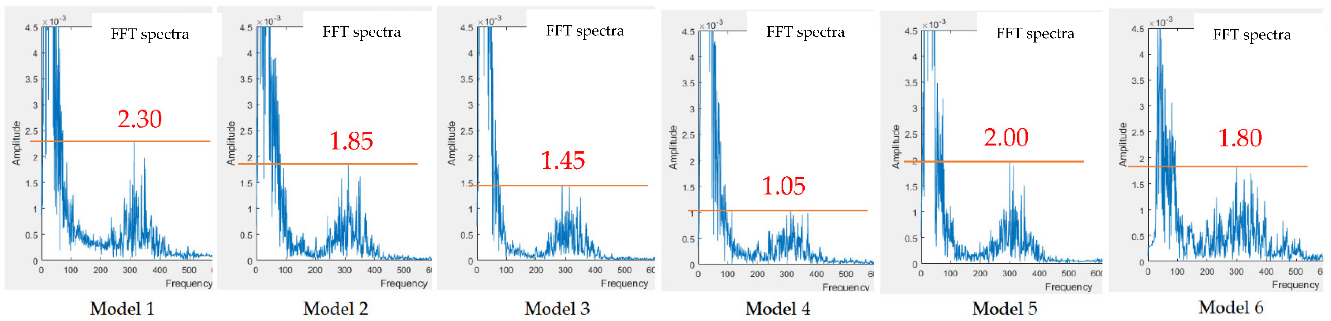
| Model 1 | Model 2 | Model 3 | Model 4 | Model 5 | |
|---|---|---|---|---|---|
| Measurement 1 | 0~100 | 0~100 | 0~100 | 0~100 | 0~100 |
| Measurement 2 | 0~100 | 0~100 | 0~100 | 0~100 | 0~100 |
| 150~450 | 150~450 | 150~450 | 150~450 | 150~450 | |
| peak at 300 | peak at 300 | peak at 300 | peak at 300 | peak at 300 | |
| Measurement 3 | 150~550 | 150~550 | 150~450 | 250~450 | |
| peak at 375 | peak at 375 | peak at 350 | peak at 350 | ||
| Measurement 4 | 0~150 | 0~150 | 0~150 | 0~150 | 0~150 |
| Measurement 5 | 0~150 | 0~150 | 0~150 | 0~150 | 0~150 |
| 200~450 | 200~400 | 240~420 | 250~400 | 250~400 | |
| peak at 325 | peak at 325 | peak at 310 | peak at 310 | peak at 310 | |
| Measurement 6 | 0~150 | 0~150 | 0~150 | 0~150 | |
| 250~450 | 250~450 | 250~450 | 250~450 |
| Model 1 | Model 2 | ||
|---|---|---|---|
| w/o subtracter | with subtracter | w/o subtracter | with subtracter |
 |  |  |  |
| Model 3 | Model 4 | ||
| w/o subtracter | with subtracter | w/o subtracter | with subtracter |
 |  |  |  |
| Training Samples | Testing Sampes | Noisy Samples | |||
|---|---|---|---|---|---|
| Abnormal | Normal | Abnormal | Normal | Abnormal | Normal |
| 411 | 1940 | 103 | 485 | 151 | 150 |
| Models | Training #: Testing # | Accuracy | Sensitivity | Specificity | F1 |
|---|---|---|---|---|---|
| Adaptive Boosting + CNN [17] | 9:1 | 86.02 | 94.24 | 77.81 | -- |
| DNN [18] | 9:1 | 97.10 | 99.26 | 94.86 | -- |
| WST + PCA + 2SVM [20] * | 7:3 | 93.06 | -- | -- | -- |
| Classic ML + DL [21] | 9:1 | 92.9 | 82.3 | 96.2 | -- |
| 1D CNN+ BiLSTM [22] | 9:1 | 86.57 | 91.78 | 59.05 | 91.78 |
| Ensemble-NN [33] | 9:1 | 91.5 | 94.23 | 88.76 | -- |
| DropConnected-NN [34] | 9:1 | 84.1 | 84.8 | 93.3 | -- |
| Adaptive Boosting + CNN [17] ** | -- | 89.6 | 93.7 | 85.6 | 90 |
| Ensemble-NN [33] ** | -- | 93.0 | 94.5 | 91.4 | 93.1 |
| DropConnected-NN [34] ** | -- | 93.1 | 94.5 | 91.7 | 93.1 |
| Presented model | 4:1 | 86.9 | 81.9 | 91.8 | 86.1 |
Publisher’s Note: MDPI stays neutral with regard to jurisdictional claims in published maps and institutional affiliations. |
© 2022 by the authors. Licensee MDPI, Basel, Switzerland. This article is an open access article distributed under the terms and conditions of the Creative Commons Attribution (CC BY) license (https://creativecommons.org/licenses/by/4.0/).
Share and Cite
Wu, Y.-C.; Han, C.-C.; Chang, C.-S.; Chang, F.-L.; Chen, S.-F.; Shieh, T.-Y.; Chen, H.-M.; Lin, J.-Y. Development of an Electronic Stethoscope and a Classification Algorithm for Cardiopulmonary Sounds. Sensors 2022, 22, 4263. https://doi.org/10.3390/s22114263
Wu Y-C, Han C-C, Chang C-S, Chang F-L, Chen S-F, Shieh T-Y, Chen H-M, Lin J-Y. Development of an Electronic Stethoscope and a Classification Algorithm for Cardiopulmonary Sounds. Sensors. 2022; 22(11):4263. https://doi.org/10.3390/s22114263
Chicago/Turabian StyleWu, Yu-Chi, Chin-Chuan Han, Chao-Shu Chang, Fu-Lin Chang, Shi-Feng Chen, Tsu-Yi Shieh, Hsian-Min Chen, and Jin-Yuan Lin. 2022. "Development of an Electronic Stethoscope and a Classification Algorithm for Cardiopulmonary Sounds" Sensors 22, no. 11: 4263. https://doi.org/10.3390/s22114263