
Spectral Analysis and Information Entropy Approaches to Data of VLF Disturbances in the Waveguide Earth-Ionosphere
 , , , , , , , and
Abstract
:1. Introduction
1.1. Factors Affecting the Propagation of VLF Signals
1.2. Main Goals of the Work
2. Data and Methods of Analysis
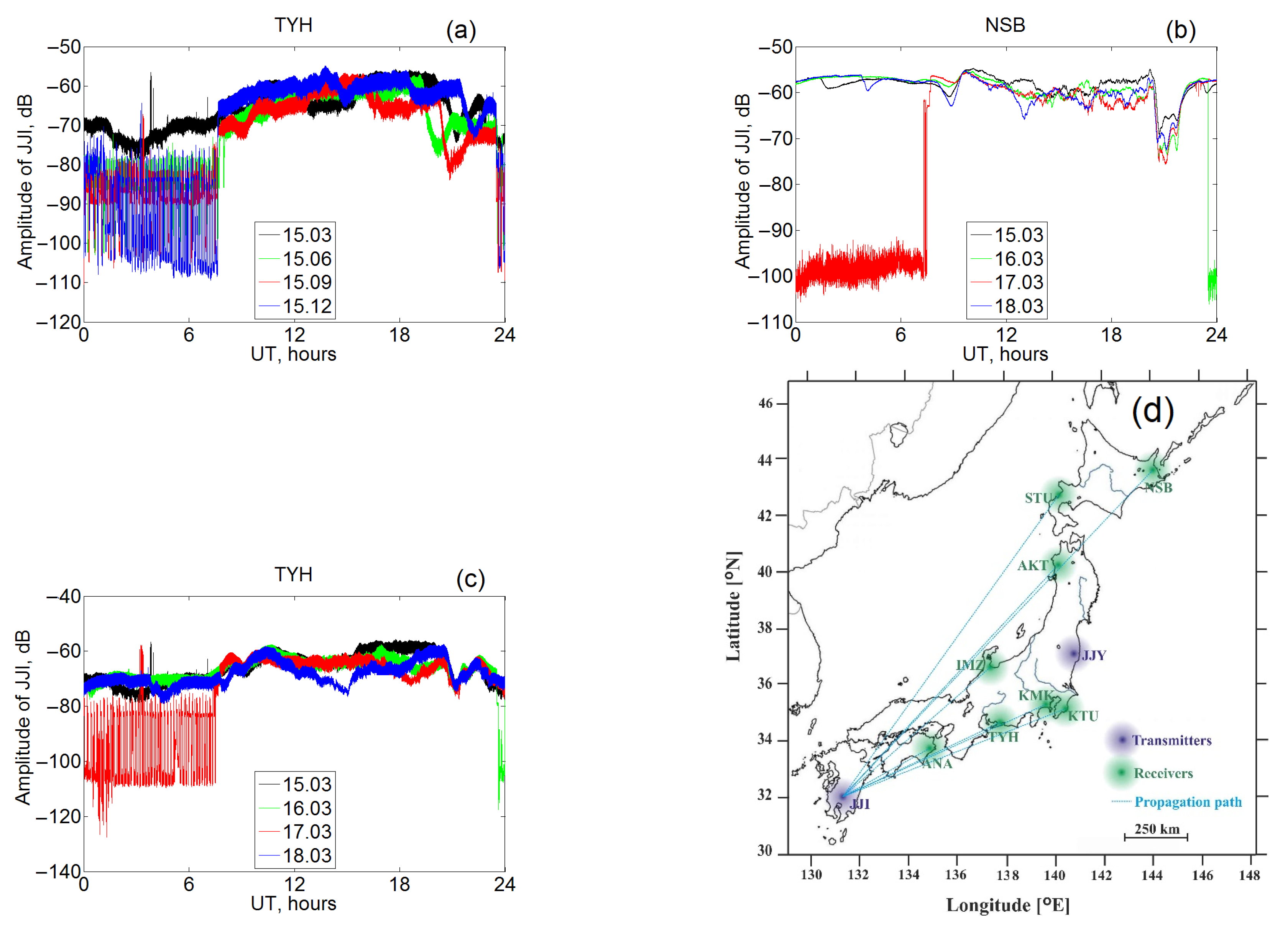
2.1. VLF Data
2.2. Methods of Analysis
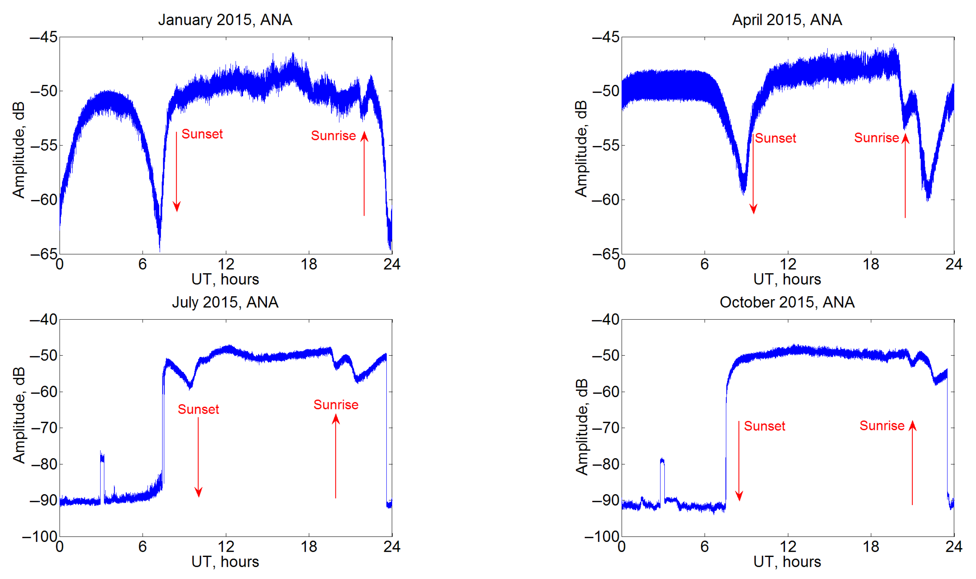
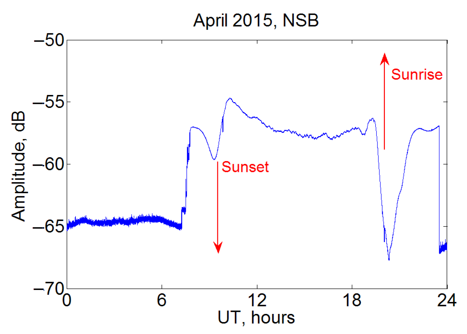
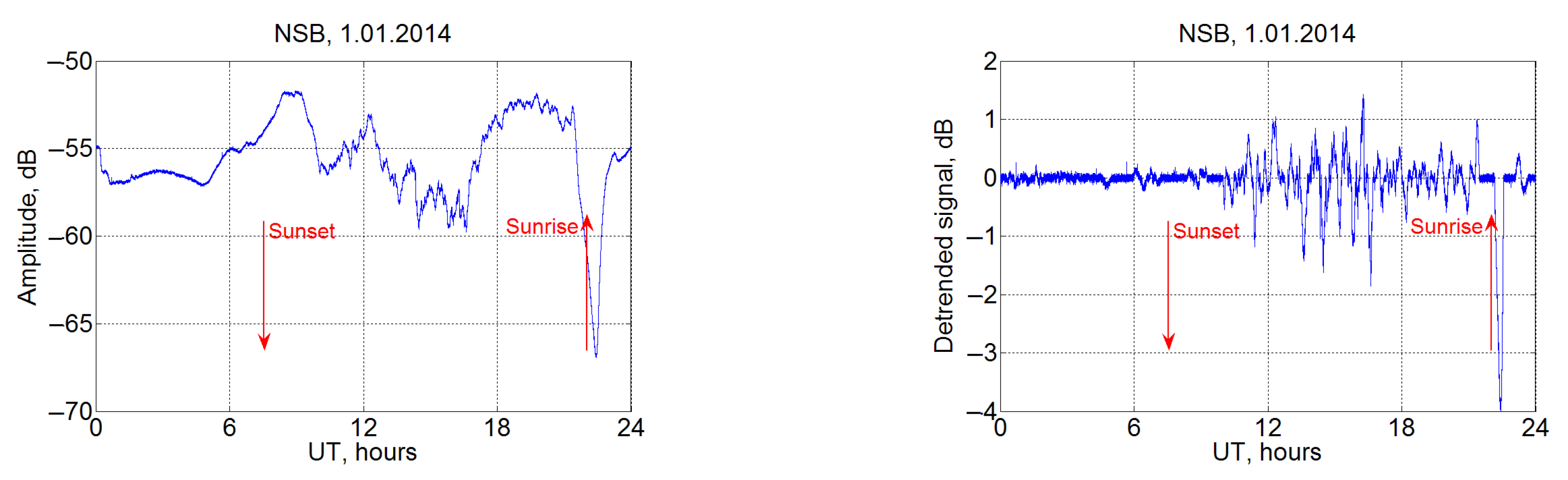
3. Daily Variations of VLF Signal Accounting for Influence of Terminator

4. Application of Information Entropy to Process VLF Signal Parameters
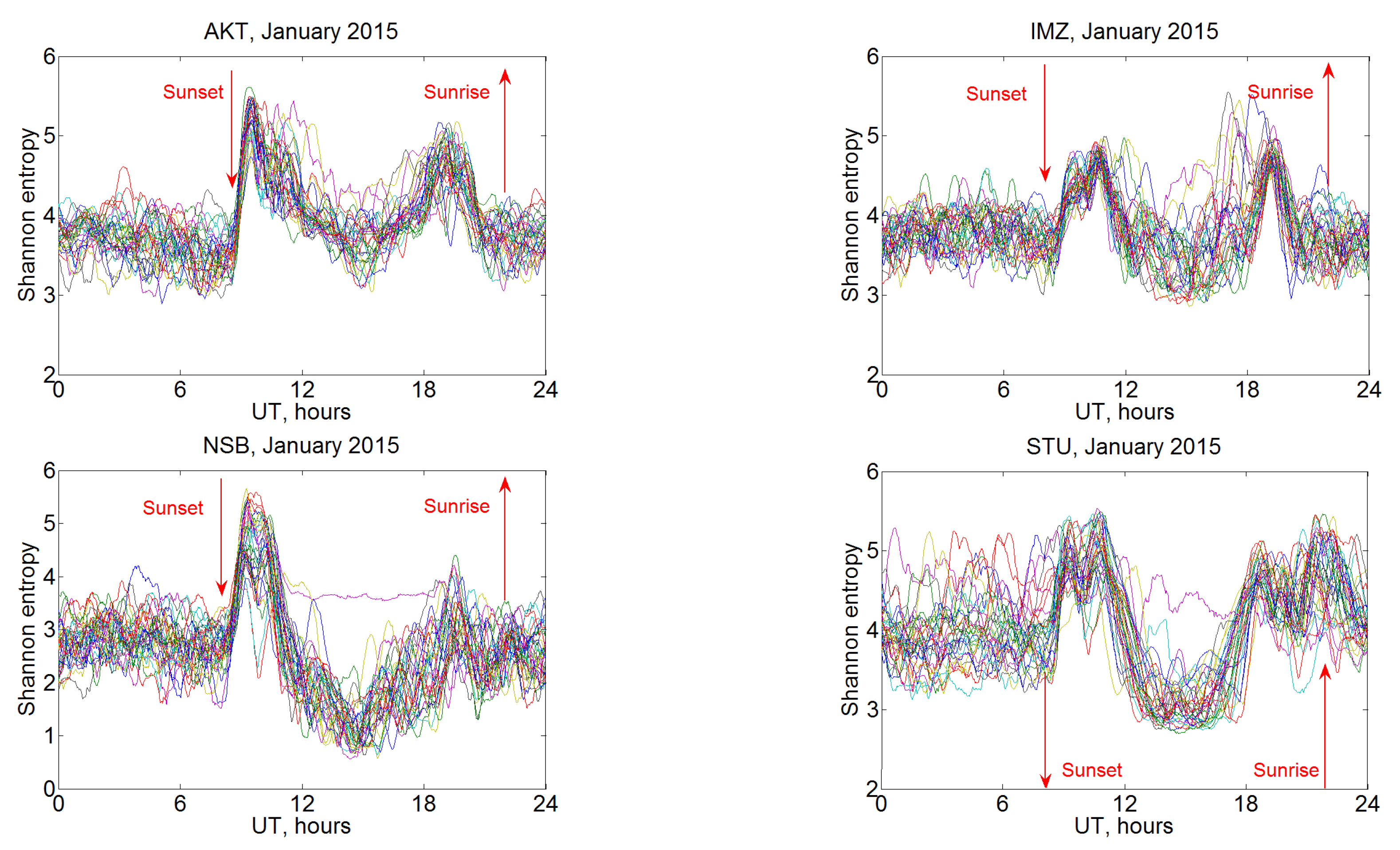
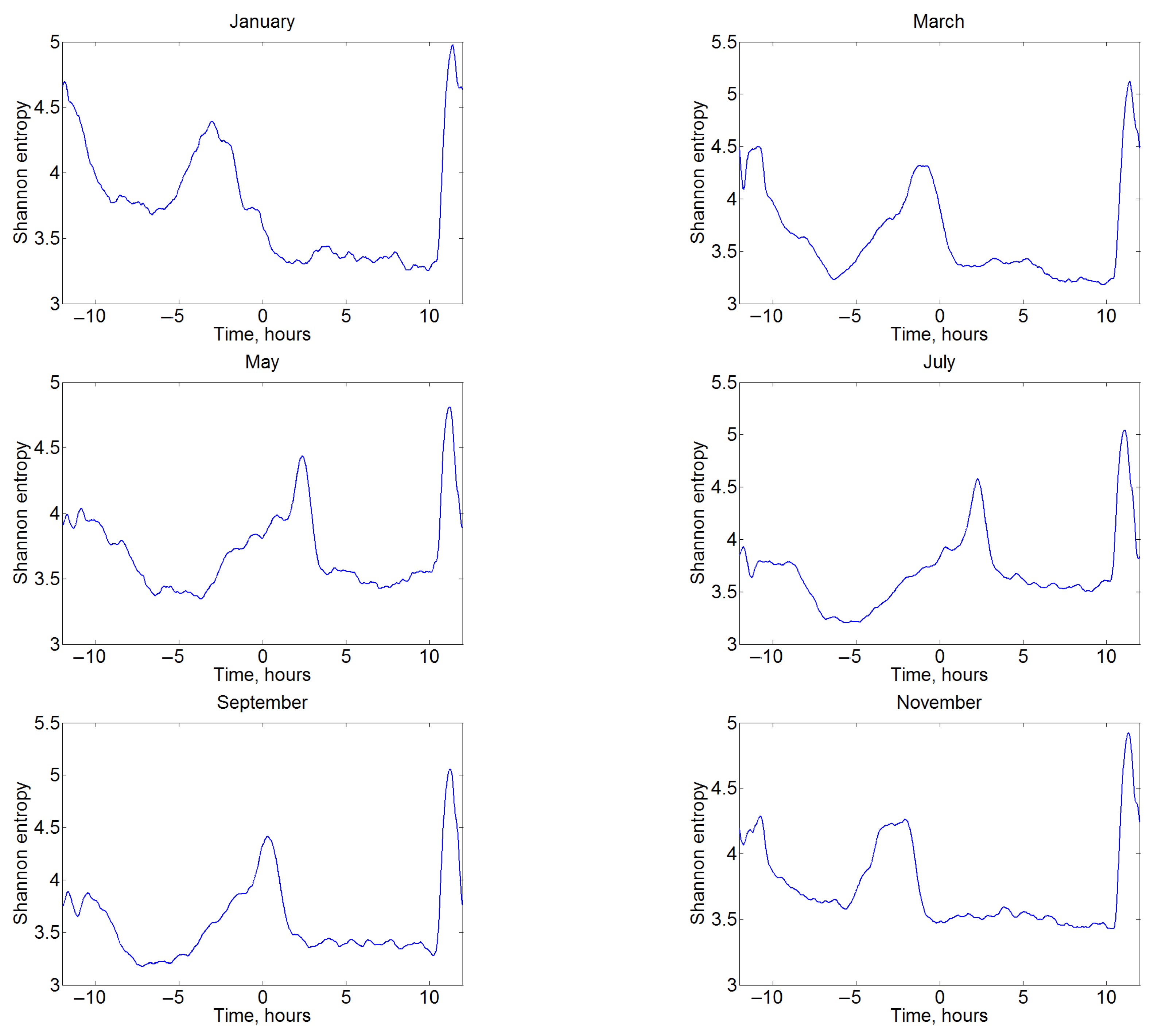
5. Daily Variations of Information Entropy, Features of the Terminator Passage
6. Discussion
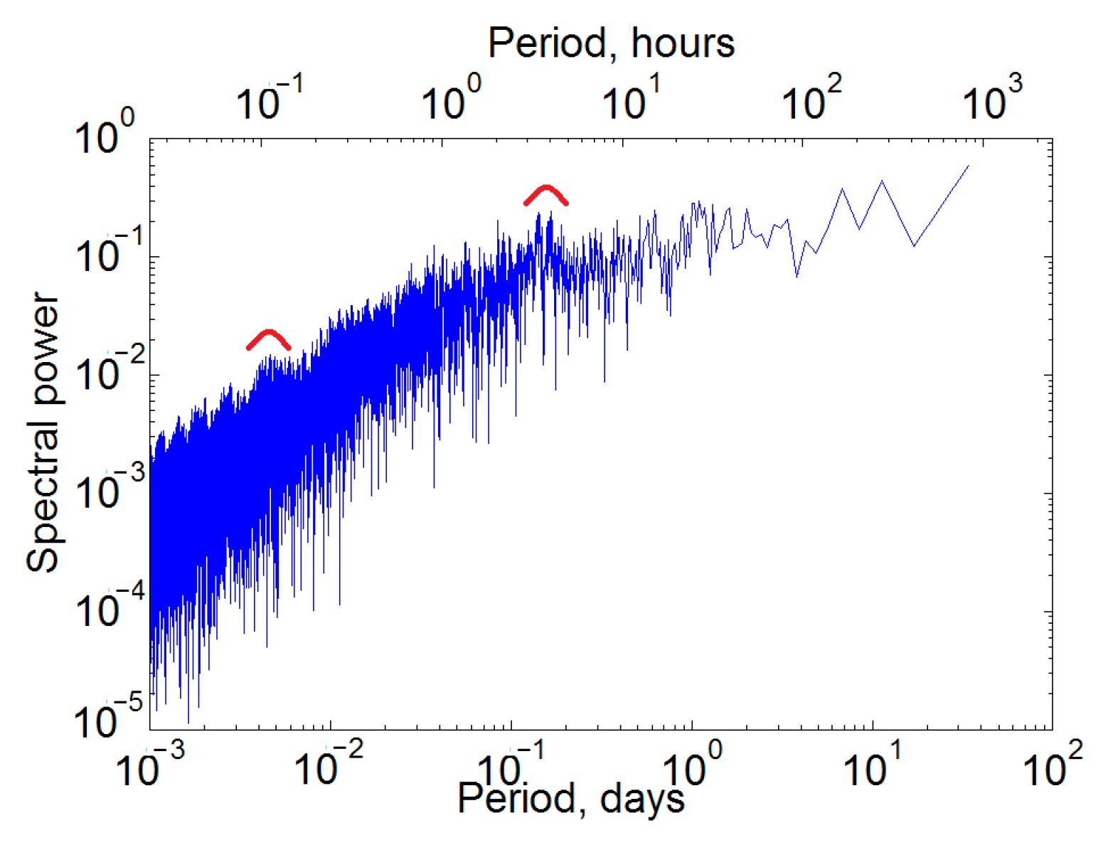
- a noticeable increase is in the spectrum at periods of 5–10 and 20–25 min, which may indicate the generation of oscillations with these periods;
- at periods of 60–70 min and 3–4 h (long-period gravity waves);
- there are also indications of a weekly trend, which may be caused by the effect of anthropogenical activities on the atmosphere/ionosphere.
7. Conclusions
- (a)
- The following variations in the VLF signals propagation in the WGEI have been revealed:
- a noticeable increase is in the spectrum at periods of 5–10 min; note that it covers the range of periods 6–7 min, which may indicate an effect on the modulation of the VLF EMW, propagating in the WGEI, caused by AGW oscillations near the Brunt–Väisälä period, i.e., a period of fundamental atmospheric fluctuations.
- quasi-wave oscillations of the received signal with periods of 20–25 and 60–70 min, which can also be associated with AGWs, i.e., disturbances in the ULF range;
- oscillations at periods of 3–4 h (probably, long-period gravity waves);
Such disturbances can be excited by solar terminator, maybe earthquakes or other sources; the details of the proper excitation mechanism(s) will be a subject of the next paper(s).A weekly trend, which may be caused due to the effect of anthropogenic activities on the atmosphere/ionosphere, is also revealed. - (b)
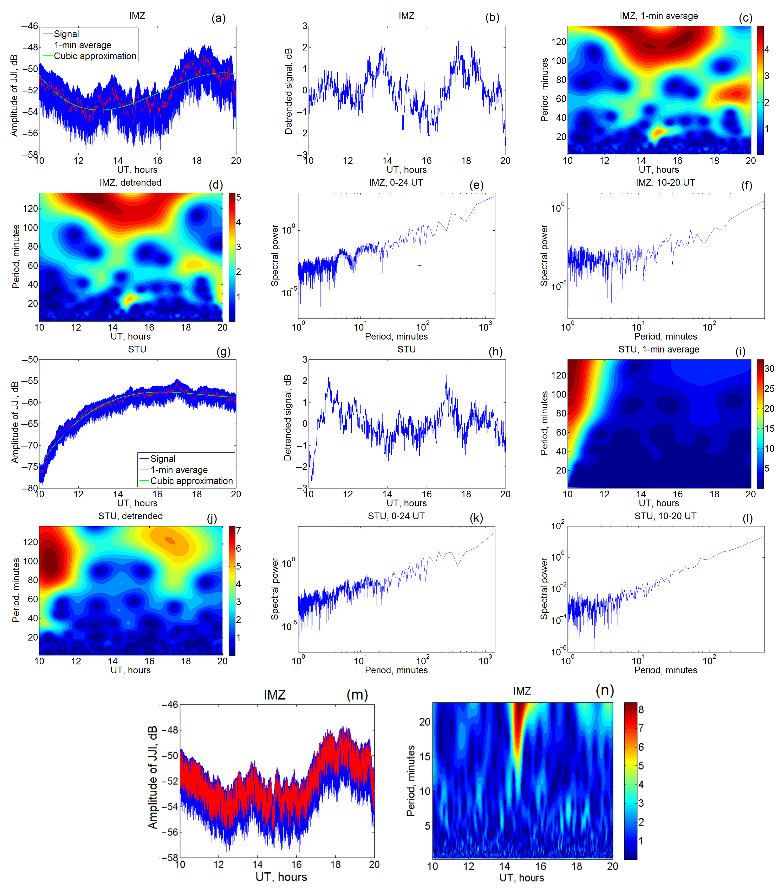
- The very effective method of spatio-temporal characteristics, in particular, of VLF perturbations in the WGEI appeared to be the combination of detrending and wavelet analysis with proper averaging. At four different receivers from the network of Japan stations, oscillations of the same periods, in particular, 20 and 60 min., have been revealed. This procedure was successful, in particular, for the STU station only with detrending and after application of wavelet analysis, while without detrending the corresponding oscillations have not been seen;
- (c)
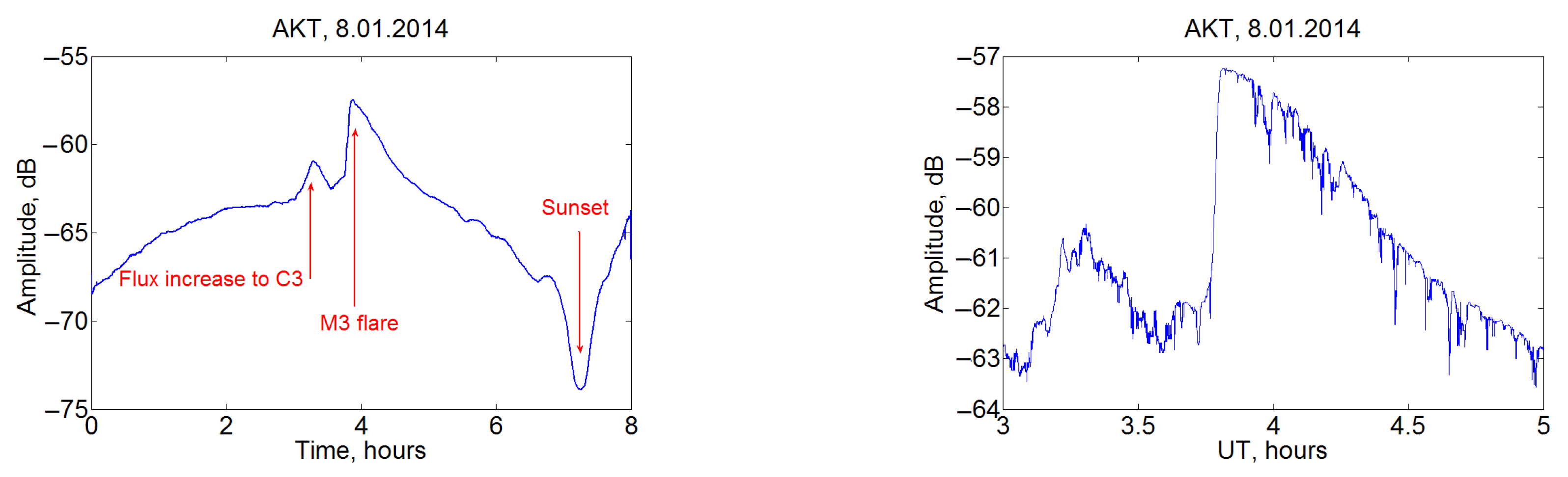
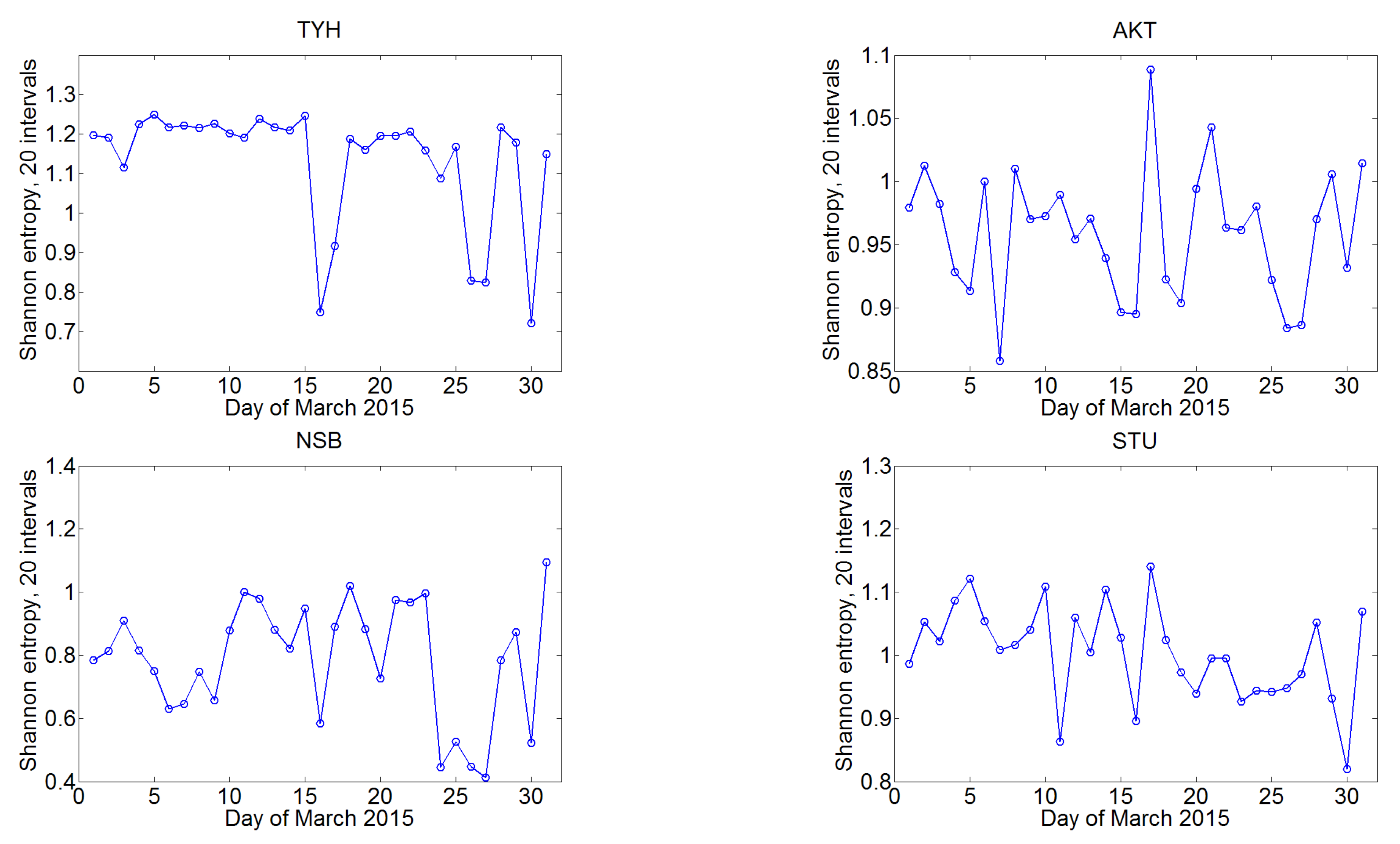
- The information entropy has been found to show maxima near sunrise and sunset, and the time of these peaks relative to the indicated moments changes with season. The effect of solar flares on information entropy has been previously established as the VLF amplitude increase, but this issue needs further study;
- (d)
- The presence of ULF modulation of the VLF EMW spectrum propagating in WGEI is qualitatively explained. The appearance of the combination frequency of VLF EMW and ULF AGW is due to the following effects: (1) the drag of charged plasma particles by ULF AGWs jointly with the background of VLF electron density disturbances and (2) the motion of charged plasma particles in the VLF EMW field jointly with the background of ULF changes in the plasma concentration caused by AGW. The features of the modulated VLF spectra found in the processing of experimental data are compared with the characteristics of various ULF oscillations of the atmosphere. They may be evanescent or reactive Lamb waves and global Brunt–Väisälä oscillations. The periods of such oscillations correspond to the spectral components that appear in the VLF EMW spectra in WGEI due to ULF modulation. These periods are 6–7 min, 20-60 min, and 3 h; the shorter period of ULF modulation of order 4 min (Figure 4n) may characterize the acoustic branch of AGW in the Earth–Thermosphere waveguide.
Author Contributions
Funding
Institutional Review Board Statement
Informed Consent Statement
Data Availability Statement
Conflicts of Interest
Appendix A
- (a)
- Influence of AGW on the ionosphere and mixing VLF EMW and ULF AGW frequencies: VLF EMW modulation by AGWs
- (b)
- The main evanescent (reactive) modes AGW in the atmosphere
References
- Kelley, M.; Heelis, R. The Earth’s Ionosphere, Plasma Physics and Electrodynamics; Elsevier: Amsterdam, The Netherlands, 1989; Volume 96. [Google Scholar]
- Hayakawa, M.; Molchanov, O.A.; Ondoh, T.; Kawai, E. On the precursory signature of Kobe earthquake on VLF subionospheric signals. In Proceedings of the International Symposium on Electromagnetic Compatibility, Beijing, China, 21–23 May 1997; pp. 72–75. [Google Scholar] [CrossRef]
- Grimalsky, V.; Hayakawa, M.; Ivchenko, V.; Rapoport, Y.; Zadorozhnii, V. Penetration of an electrostatic field from the lithosphere into the ionosphere and its effect on the D-region before earthquakes. J. Atmos. Sol. -Terr. Phys. 2003, 65, 391–407. [Google Scholar] [CrossRef]
- Boudjada, M.Y.; Schwingenschuh, K.; Döller, R.; Rohznoi, A.; Parrot, M.; Biagi, P.F.; Galopeau, P.H.M.; Solovieva, M.; Molchanov, O.; Biernat, H.K.; et al. Decrease of VLF transmitter signal and Chorus-whistler waves before l’Aquila earthquake occurrence. Nat. Hazards Earth Syst. Sci. 2010, 10, 1487–1494. [Google Scholar] [CrossRef] [Green Version]
- Inan, U.S.; Cummer, S.A.; Marshall, R.A. A survey of ELF and VLF research on lightning-ionosphere interactions and causative discharges. J. Geophys. Res. Space Phys. 2010, 115. [Google Scholar] [CrossRef] [Green Version]
- Titova, E.E.; Di, V.I.; Yurov, V.E.; Raspopov, O.M.; Trakhtengertz, V.Y.; Jiricek, F.; Triska, P. Interaction between VLF waves and the turbulent ionosphere. Geophys. Res. Lett. 1984, 11, 323–326. [Google Scholar] [CrossRef]
- Gross, N.C.; Cohen, M.B.; Said, R.K.; Gołkowski, M. Polarization of Narrowband VLF Transmitter Signals as an Ionospheric Diagnostic. J. Geophys. Res. Space Phys. 2018, 123, 901–917. [Google Scholar] [CrossRef]
- Davies, K. Ionospheric Radio; IEEE Electromagnetic Waves Series 31; Peter Peregrinus Ltd.: London, UK, 1990; 580p. [Google Scholar]
- McRae, W.M.; Thomson, N.R. VLF phase and amplitude: Daytime ionospheric parameters. J. Atmos. Sol. Terr. Phys. 2000, 62, 609–618. [Google Scholar] [CrossRef]
- Hegde, S.; Bobra, M.G.; Scherrer, P.H. Classifying Signatures of Sudden Ionospheric Disturbances. Res. Notes AAS 2018, 2, 162. [Google Scholar] [CrossRef]
- Macotela, E.L.; Raulin, J.P.; Manninen, J.; Correia, E.; Turunen, T.; Magalhães, A. Lower Ionosphere Sensitivity to Solar X-ray Flares Over a Complete Solar Cycle Evaluated From VLF Signal Measurements. J. Geophys. Res. Space Phys. 2017, 122, 370–377. [Google Scholar] [CrossRef] [Green Version]
- Barghi, W.; Delavar, M.; Shahabadi, M.; Zare, M.; Eslaminezhad, S.A.; Bayat, H. Earthquake prediction evaluation based on VLF data using a novel intersection-union method. ISPRS Ann. Photogramm. Remote Sens. Spat. Inf. Sci. 2021, V-4, 25–32. [Google Scholar] [CrossRef]
- Rozhnoi, A.; Solovieva, M.; Parrot, M.; Hayakawa, M.; Biagi, P.F.; Schwingenschuh, K.; Fedun, V. VLF/LF signal studies of the ionospheric response to strong seismic activity in the Far Eastern region combining the DEMETER and ground-based observations. Phys. Chem. Earth Parts A/B/C 2015, 85–86, 141–149. [Google Scholar] [CrossRef]
- Popova, I.; Rozhnoi, A.; Solovieva, M.; Chebrov, D.; Hayakawa, M. The Behavior of VLF/LF Variations Associated with Geomagnetic Activity, Earthquakes, and the Quiet Condition Using a Neural Network Approach. Entropy 2018, 20, 691. [Google Scholar] [CrossRef] [PubMed] [Green Version]
- Ouzounov, D.; Pulinets, S.; Davidenko, D.; Rozhnoi, A.; Solovieva, M.; Fedun, V.; Dwivedi, B.N.; Rybin, A.; Kafatos, M.; Taylor, P. Transient Effects in Atmosphere and Ionosphere Preceding the 2015 M7.8 and M7.3 Gorkha–Nepal Earthquakes. Front. Earth Sci. 2021, 9. [Google Scholar] [CrossRef]
- Hayakawa, M. Earthquake Prediction with Radio Techniques; Wiley: Hoboken, NJ, USA, 2015; pp. 1–294. [Google Scholar] [CrossRef]
- Nina, A.; Radovanović, M.; Milovanović, B.; Kovačević, A.; Bajčetić, J.; Popović, L.Č. Low ionospheric reactions on tropical depressions prior hurricanes. Adv. Space Res. 2017, 60, 1866–1877. [Google Scholar] [CrossRef] [Green Version]
- Pulinets, S.; Ouzounov, D. The Possibility of Earthquake Forecasting; IOP Publishing: Bristol. UK, 2018; pp. 2053–2563. [Google Scholar] [CrossRef]
- Rapoport, Y.; Gotynyan, O.; Ivchenko, V.; Kozak, L.; Parrot, M. Effect of acoustic-gravity wave of the lithospheric origin on the ionospheric F region before earthquakes. Phys. Chem. Earth Parts A/B/C 2004, 29, 607–616. [Google Scholar] [CrossRef]
- Rapoport, Y.; Hayakawa, M.; Gotynyan, O.; Ivchenko, V.; Fedorenko, A.; Selivanov, Y. Stable and unstable plasma perturbations in the ionospheric F region, caused by spatial packet of atmospheric gravity waves. Phys. Chem. Earth Parts A/B/C 2009, 34, 508–515. [Google Scholar] [CrossRef]
- Rapoport, Y.; Grimalsky, V.; Krankowski, A.; Pulinets, S.; Fedorenko, A.; Petrishchevskii, S. Algorithm for modeling electromagnetic channel of seismo-ionospheric coupling (SIC) and the variations in the electron concentration. Acta Geophys. 2019, 68, 253–278. [Google Scholar] [CrossRef]
- Yoshida, M.; Yamauchi, T.; Horie, T.; Hayakawa, M. On the generation mechanism of terminator times in subionospheric VLF/LF propagation and its possible application to seismogenic effects. Nat. Hazards Earth Syst. Sci. 2008, 8, 129–134. [Google Scholar] [CrossRef]
- Fedorenko, A.K.; Kryuchkov, E.I.; Cheremnykh, O.K.; Zhuk, I.T.; Voitsekhovska, A.D. Studies of wave disturbances in the mid-latitude mesosphere on VLF radio network data. Space Sci. Technol. 2019, 25, 48–61. [Google Scholar] [CrossRef]
- Fedorenko, A.K.; Kryuchkov, E.I.; Cheremnykh, O.K.; Voitsekhovska, A.D.; Rapoport, Y.G.; Klymenko, Y.O. Analysis of acoustic-gravity waves in the mesosphere using VLF radio signal measurements. J. Atmos. Sol. Terr. Phys. 2021, 219, 105649. [Google Scholar] [CrossRef]
- Meng, X.; Verkhoglyadova, O.P.; Komjathy, A.; Savastano, G.; Mannucci, A.J. Physics-Based Modeling of Earthquake-Induced Ionospheric Disturbances. J. Geophys. Res. Space Phys. 2018, 123, 8021–8038. [Google Scholar] [CrossRef]
- Koshovyi, V.V.; Soroka, S.O. Acoustic Disturbance of Ionospheric Plasma by a Ground-Based Radiator. Kosm. Nauka Tekhnologiya 1998, 4, 3–17. [Google Scholar] [CrossRef]
- Kotsarenko, N.Y.; Soroka, S.A.; Koshevaya, S.V.; Koshovy, V.V. Increase of the Transparency of the Ionosphere for Cosmic Radiowaves Caused by a Low Frequency Wave. Phys. Scr. 1999, 59, 174–181. [Google Scholar] [CrossRef]
- Grimalsky, V.V.; Koshevaya, S.V.; Perez-Enriquez, R.; Kotsarenko, A.N. Nonlinear Excitation of ULF Atmosphere–Ionosphere Waves and Magnetic Perturbations Caused by ELF Seismic Acoustic Bursts. Phys. Scr. 2003, 67, 453–456. [Google Scholar] [CrossRef]
- Krasnov, V.; Kuleshov, Y. Variation of Infrasonic Signal Spectrum during Wave Propagation from Earth’s Surface to Ionospheric Altitudes. Acoust. Physi. 2014, 60, 19–28. [Google Scholar] [CrossRef]
- Rapoport, Y.; Cheremnykh, O.; Koshovyy, V.; Melnik, M.; Ivantyshyn, O.; Nogach, R.; Selivanov, Y.; Grimalsky, V.; Mezentsev, V.; Karataeva, L.; et al. Ground-based acoustic parametric generator impact on the atmosphere and ionosphere in an active experiment. Ann. Geophys. 2017, 35, 53–70. [Google Scholar] [CrossRef] [Green Version]
- Grimalsky, V.; Rapoport, Y.; Tecpoyotl-Torres, M.; Ivantyshyn, O.; Nesterenko, A. Nonlinear frequency down-conversion of acoustic wave beams in the atmosphere and ionosphere under different types of modulation (regular item). J. Atmos. Sol. Terr. Phys. 2022, 227, 105774. [Google Scholar] [CrossRef]
- Silber, I.; Price, C. On the Use of VLF Narrowband Measurements to Study the Lower Ionosphere and the Mesosphere–Lower Thermosphere. Surv. Geophys. 2017, 38, 1–35. [Google Scholar] [CrossRef]
- Haken, H.; Fraser, A.M. Information and Self-Organization: A Macroscopic Approach to Complex Systems. Am. J. Phys. 1989, 57, 958–959. [Google Scholar] [CrossRef] [Green Version]
- De Santis, A.; Abbattista, C.; Alfonsi, L.; Amoruso, L.; Campuzano, S.A.; Carbone, M.; Cesaroni, C.; Cianchini, G.; De Franceschi, G.; De Santis, A.; et al. Geosystemics View of Earthquakes. Entropy 2019, 21, 412. [Google Scholar] [CrossRef] [Green Version]
- Guglielmi, A.V.; Pokhotelov, O.A. Geoelectromagnetic Waves; Institute of Physics Publishing: Bristol, UK; Philadelphia, PA, USA, 1996; Volume 61, p. 382. [Google Scholar] [CrossRef]
- Potirakis, S.; Minadakis, G.; Eftaxias, K. Relation between seismicity and pre-earthquake electromagnetic emissions in terms of energy, information and entropy content. Nat. Hazards Earth Syst. Sci. 2012, 12, 1179–1183. [Google Scholar] [CrossRef] [Green Version]
- Asano, T.; Hayakawa, M. On the Tempo-Spatial Evolution of the Lower Ionospheric Perturbation for the 2016 Kumamoto Earthquakes from Comparisons of VLF Propagation Data Observed at Multiple Stations with Wave-Hop Theoretical Computations. Open J. Earthq. Res. 2018, 7, 161–185. [Google Scholar] [CrossRef] [Green Version]
- Politis, D.Z.; Potirakis, S.M.; Contoyiannis, Y.F.; Biswas, S.; Sasmal, S.; Hayakawa, M. Statistical and Criticality Analysis of the Lower Ionosphere Prior to the 30 October 2020 Samos (Greece) Earthquake (M6.9), Based on VLF Electromagnetic Propagation Data as Recorded by a New VLF/LF Receiver Installed in Athens (Greece). Entropy 2021, 23, 676. [Google Scholar] [CrossRef] [PubMed]
- Haken, H. Synergetics: An Introduction; Springer: Berlin, Germany, 1978. [Google Scholar]
- Shannon, C.E. A mathematical theory of communication. Bell Syst. Technical J. 1948, 27, 379–423. [Google Scholar] [CrossRef] [Green Version]
- De Santis, A.; Cianchini, G.; Favali, P.; Beranzoli, L.; Boschi, E. The Gutenberg–Richter Law and Entropy of Earthquakes: Two Case Studies in Central Italy. Bull. Seismol. Soc. Am. 2011, 101, 1386–1395. [Google Scholar] [CrossRef]
- Pulinets, S. The synergy of earthquake precursors. Acta Seismol. Sin. 2011, 24, 535–548. [Google Scholar] [CrossRef] [Green Version]
- Chernogor, L.F.; Rozumenko, V.T. Earth-Atmosphere-Geospace as an Open Nonlinear Dynamical System. Russ. Radio Phys. Radio Astron. 2008, 13, 120. [Google Scholar]
- Potirakis, S.M.; Asano, T.; Hayakawa, M. Criticality Analysis of the Lower Ionosphere Perturbations Prior to the 2016 Kumamoto (Japan) Earthquakes as Based on VLF Electromagnetic Wave Propagation Data Observed at Multiple Stations. Entropy 2018, 20, 199. [Google Scholar] [CrossRef]
- Asano, T.; Rozhnoi, A.; Solovieva, M.; Hayakawa, M. Characteristic Variations of VLF/LF Signals during a High Seismic Activity in Japan in November 2016. Open J. Earthq. Res. 2017, 6, 204–215. [Google Scholar] [CrossRef] [Green Version]
- Rozhnoi, A.; Solovieva, M.; Molchanov, O.; Schwingenschuh, K.; Boudjada, M.; Biagi, P.F.; Maggipinto, T.; Castellana, L.; Ermini, A.; Hayakawa, M. Anomalies in VLF radio signals prior the Abruzzo earthquake (M = 6.3) on 6 April 2009. Nat. Hazards Earth Syst. Sci. 2009, 9, 1727–1732. [Google Scholar] [CrossRef] [Green Version]
- Kasahara, Y.; Nakamura, T.; Hobara, Y.; Hayakawa, M.; Rozhnoi, A.; Solovieva, M.; Molchanov, O. A statistical study on the AGW modulations in subionospheric VLF/LF propagation data and consideration of the generation mechanism of seismo-ionospheric perturbations. J. Atmos. Electr. 2010, 30, 103–112. [Google Scholar] [CrossRef] [Green Version]
- Torrence, C.; Compo, G.P. A Practical Guide to Wavelet Analysis. Bull. Am. Meteorol. Soc. 1998, 79, 61–78. [Google Scholar] [CrossRef]
- Krishnan, V. Probability and Random Processes; Wiley: Hoboken, NJ, USA, 2006. [Google Scholar] [CrossRef]
- Sharma, A.; More, C. Diurnal Variation of VLF Radio Wave Signal Strength at 19.8 and 24 kHz Received at Khatav India (16°46′ N, 75°53′ E). Res. Rev. J. Space Sci. Technol. 2017, 6, 1–12. [Google Scholar]
- Hooke, W.H. Gravity Waves. In Mesoscale Meteorology and Forecasting; American Meteorological Society: Boston, MA, USA, 1986; pp. 272–288. [Google Scholar] [CrossRef]
- Erokhin, N.S.; Zolnikova, N.; Mikhailovskaya, L. Peculiarities of the interaction of internal gravity waves with the temperature-wind structures of the atmosphere during propagation into the ionosphere. Curr. Probl. Remote. Sens. Earth Space 2007, 2, 82–84. [Google Scholar]
- Gossard, E.; Hooke, W. Waves in the Atmosphere; Elsevier: Amsterdam, The Netherlands, 1975; p. 456. [Google Scholar]
- Nina, A.; Čadež, V.M. Detection of acoustic-gravity waves in lower ionosphere by VLF radio waves. Geophys. Res. Lett. 2013, 40, 4803–4807. [Google Scholar] [CrossRef] [Green Version]
- Beer, T. Atmospheric Waves; Wiley: New York, NY, USA, 1974. [Google Scholar]
- Gotynyan, O.E.; Ivchenko, V.N.; Rapoport, Y.G. Model of the internal gravity waves excited by lithospheric greenhouse effect gases. Kosm. Nauka Tekhnologiya 2001, 7, 26–33. [Google Scholar] [CrossRef]
- Rapoport, Y.G. General method for the derivations of the evolution equations and modeling. Bullet. Taras Shevchenko Nat. Univ. Kyiv Ser. Phys. Math. 2014, 1, 281–288. [Google Scholar]
- Walterscheid, R.L.; Hecht, J.H. A reexamination of evanescent acoustic-gravity waves: Special properties and aeronomical significance. J. Geophys. Res. Atmos 2003, 108. Available online: http://xxx.lanl.gov/abs/https://agupubs.onlinelibrary.wiley.com/doi/pdf/10.1029/2002JD002421 (accessed on 18 October 2022). [CrossRef]
- Cheremnykh, O. Resonant mode in the Earth’s thermosphere. Kosm. Nauka Tekhnologiya 2011, 6, 74–76. [Google Scholar] [CrossRef]
- Gotynyan, O.; Ivchenko, V.; Rapoport, Y.; Parrot, M. Ionospheric disturbances excited by the lithospheric gas source of acoustic gravity waves before eartquakes. Kosm. Nauka Tekhnologiya 2002, 8, 89–105. [Google Scholar] [CrossRef]
- Rapoport, Y.; Grimalsky, V.; Fedun, V.; Agapitov, O.; Bonnell, J.; Grytsai, A.; Milinevsky, G.; Liashchuk, A.; Rozhnoi, A.; Solovieva, M.; et al. Model of Propagation of VLF Beams in the Waveguide Earth-Ionosphere. Principles of Tensor Impedance Method in Multilayered Gyrotropic Waveguides. Ann. Geophys. Discuss. 2019, 38, 1–31. [Google Scholar] [CrossRef] [Green Version]
- Bryunelli, B.; Namgaladze, A. Physics of the Ionosphere; Nauka: Moscow, Russia, 1988. [Google Scholar]
- Hines, C.O. Internal atmospheric gravity waves at ionospheric heights. Can. J. Phys. 1960, 38, 1441–1481. [Google Scholar] [CrossRef]
- Simpson, J.; Halverson, J.B.; Ferrier, B.S.; Petersen, W.A.; Simpson, R.H.; Blakeslee, R.J.; Durden, S.L. On the role of “hot towers” in tropical cyclone formation. Meteorol. Atmos. Phys. 1998, 67, 15–35. [Google Scholar] [CrossRef]
- Qie, X.; Liu, D.; Sun, Z. Recent advances in research of lightning meteorology. J. Meteorol. Res. 2014, 28, 983–1002. [Google Scholar] [CrossRef]
- Sorokin, V.M.; Yaschenko, A.K.; Hayakawa, M. A perturbation of DC electric field caused by light ion adhesion to aerosols during the growth in seismic-related atmospheric radioactivity. Nat. Hazards Earth Syst. Sci. 2007, 7, 155–163. [Google Scholar] [CrossRef]
- Kakinami, Y.; Kamogawa, M.; Tanioka, Y.; Watanabe, S.; Gusman, A.R.; Liu, J.Y.; Watanabe, Y.; Mogi, T. Tsunamigenic ionospheric hole. Geophys. Res. Lett. 2012, 39. [Google Scholar] [CrossRef]
- Song, Q.; Ding, F.; Wan, W.; Ning, B.; Liu, L.; Zhao, B.; Li, Q.; Zhang, R. Statistical study of large-scale traveling ionospheric disturbances generated by the solar terminator over China. J. Geophys. Res. Space Phys. 2013, 118, 4583–4593. [Google Scholar] [CrossRef]
- Parrot, M.; Valerio, T.; Liu, J.; Pulinets, S.; Ouzounov, D.; Genzano, N.; Lisi, M.; Hattori, K.; Namgaladze, A. Atmospheric and ionospheric coupling phenomena related to large earthquakes. Nat. Hazards Earth Syst. Sci. Discuss. 2016, 1–30. [Google Scholar] [CrossRef] [Green Version]
- Grimalsky, V.; Rapoport, Y.; Slavin, A. Nonlinear Diffraction of Magnetostatic Waves in Ferrite Films. J. Phys. IV France 1997, 7, C1-393. [Google Scholar] [CrossRef]
- Watada, S.; Kanamori, H. Acoustic resonant oscillations between the atmosphere and the solid earth during the 1991 Mt. Pinatubo eruption. J. Geophys. Res. Solid Earth 2010, 115. [Google Scholar] [CrossRef]
- Thomas, J.N.; Huard, J.; Masci, F. A statistical study of global ionospheric map total electron content changes prior to occurrences of M ≥ 6.0 earthquakes during 2000–2014. J. Geophys. Res. Space Phys. 2017, 122, 2151–2161. [Google Scholar] [CrossRef]
- van Haarlem, M.P.; Wise, M.W.; Gunst, A.W.; Heald, G.; McKean, J.P.; Hessels, J.W.T.; de Bruyn, A.G.; Nijboer, R.; Swinbank, J.; Fallows, R.; et al. LOFAR: The LOw-Frequency ARray. Astron. Astrophys. 2013, 556, A2. [Google Scholar] [CrossRef] [Green Version]
- Dewdney, P.E.; Hall, P.J.; Schilizzi, R.T.; Lazio, T.J.L.W. The Square Kilometre Array. IEEE Proc. 2009, 97, 1482–1496. [Google Scholar] [CrossRef]
- Fallows, R.A.; Forte, B.; Astin, I.; Allbrook, T.; Arnold, A.; Wood, A.; Dorrian, G.; Mevius, M.; Rothkaehl, H.; Matyjasiak, B.; et al. A LOFAR observation of ionospheric scintillation from two simultaneous travelling ionospheric disturbances. J. Space Weather Space Clim. 2020, 10, 10. [Google Scholar] [CrossRef] [Green Version]
- Akhoondzadeh, M.; De Santis, A.; Marchetti, D.; Wang, T. Developing a Deep Learning-Based Detector of Magnetic, Ne, Te and TEC Anomalies from Swarm Satellites: The Case of Mw 7.1 2021 Japan Earthquake. Remote. Sens. 2022, 14, 1582. [Google Scholar] [CrossRef]
- Yutsis, V.; Rapoport, Y.; Grimalsky, V.; Grytsai, A.; Ivchenko, V.; Petrishchevskii, S.; Fedorenko, A.; Krivodubskij, V. ULF Activity in the Earth Environment: Penetration of Electric Field from the Near-Ground Source to the Ionosphere under Different Configurations of the Geomagnetic Field. Atmosphere 2021, 12, 801. [Google Scholar] [CrossRef]
- Alperovich, L.; Fedorov, E. Hydromagnetic Waves in the Magnetosphere and Ionosphere; Springer: Berlin, Germany, 2007; Volume 353. [Google Scholar] [CrossRef] [Green Version]
- Vainshtein, L.A. Electromagnetic Waves (2nd Revised and Enlarged Edition); Radio Sviaz: Moscow, Russia, 1988. [Google Scholar]
- Collin, R.E. Field Theory of Guided Waves, 2nd ed.; IEEE-Press: Piscataway, NJ, USA, 1991. [Google Scholar]
- Boardman, A.D.; Alberucci, A.; Assanto, G.; Rapoport, Y.G.; Grimalsky, V.V.; Ivchenko, V.M.; Tkachenko, E.N. Spatial Solitonic and Nonlinear Plasmonic Aspects of Metamaterials. In World Scientific Handbook of Metamaterials and Plasmonics; World Scientific: Singapore, 2017; Chapter 10; pp. 419–469. [Google Scholar] [CrossRef]
- Barybin, A.A. Electrodynamics of Waveguiding Structures; Fizmatlit: Moscow, Russia, 2007; p. 512. (In Russian) [Google Scholar]


| Name of Receiving Station | Latitude [°] | Longitude [°] |
|---|---|---|
| AKT | 40.10 | 140.08 |
| ANA | 33.90 | 134.67 |
| IMZ | 36.79 | 137.07 |
| KMK | 35.31 | 139.55 |
| KTU | 35.15 | 140.31 |
| NSB | 43.54 | 144.98 |
| STU | 42.80 | 140.23 |
| TYH | 34.74 | 137.37 |
Publisher’s Note: MDPI stays neutral with regard to jurisdictional claims in published maps and institutional affiliations. |
© 2022 by the authors. Licensee MDPI, Basel, Switzerland. This article is an open access article distributed under the terms and conditions of the Creative Commons Attribution (CC BY) license (https://creativecommons.org/licenses/by/4.0/).
Share and Cite
Rapoport, Y.; Reshetnyk, V.; Grytsai, A.; Grimalsky, V.; Liashchuk, O.; Fedorenko, A.; Hayakawa, M.; Krankowski, A.; Błaszkiewicz, L.; Flisek, P. Spectral Analysis and Information Entropy Approaches to Data of VLF Disturbances in the Waveguide Earth-Ionosphere. Sensors 2022, 22, 8191. https://doi.org/10.3390/s22218191
Rapoport Y, Reshetnyk V, Grytsai A, Grimalsky V, Liashchuk O, Fedorenko A, Hayakawa M, Krankowski A, Błaszkiewicz L, Flisek P. Spectral Analysis and Information Entropy Approaches to Data of VLF Disturbances in the Waveguide Earth-Ionosphere. Sensors. 2022; 22(21):8191. https://doi.org/10.3390/s22218191
Chicago/Turabian StyleRapoport, Yuriy, Volodymyr Reshetnyk, Asen Grytsai, Volodymyr Grimalsky, Oleksandr Liashchuk, Alla Fedorenko, Masashi Hayakawa, Andrzej Krankowski, Leszek Błaszkiewicz, and Paweł Flisek. 2022. "Spectral Analysis and Information Entropy Approaches to Data of VLF Disturbances in the Waveguide Earth-Ionosphere" Sensors 22, no. 21: 8191. https://doi.org/10.3390/s22218191