
Effect of Exposure Time on Thermal Behaviour: A Psychophysiological Approach
by
 , and
, and
Bilge Kobas
1,*, 
Sebastian Clark Koth
1 ,
,
Kizito Nkurikiyeyezu
2,3, 
Giorgos Giannakakis
4,5 and
and
Thomas Auer
1
1
Chair of Building Technology and Climate Responsive Design, Department of Architecture, Technical University of Munich, 80333 Munich, Germany
2
Wearable Environment and Information Systems Laboratory, Aoyama Gakuin University, 5-10-1 Fuchinobe, Chuo-ku, Sagamihara 252-5258, Japan
3
Center of Excellence in Biomedical Engineering, University of Rwanda, KN 67 Street Nyarugenge, Kigali P.O. Box 4285, Rwanda
4
Institute of Computer Science, Foundation for Research and Technology Hellas, 70013 Heraklion, Greece
5
Institute of AgriFood and Life Sciences, University Research Centre, Hellenic Mediterranean University, 71410 Heraklion, Greece
*
Author to whom correspondence should be addressed.
Signals 2021, 2(4), 863-885; https://doi.org/10.3390/signals2040050
Submission received: 31 October 2021
/
Revised: 22 November 2021
/
Accepted: 23 November 2021
/
Published: 2 December 2021
(This article belongs to the Special Issue Biosignals Processing and Analysis in Biomedicine)
Abstract
:This paper presents the findings of a 6-week long, five-participant experiment in a controlled climate chamber. The experiment was designed to understand the effect of time on thermal behaviour, electrodermal activity (EDA) and the adaptive behavior of occupants in response to a thermal non-uniform indoor environment were continuously logged. The results of the 150 h-long longitudinal study suggested a significant difference in tonic EDA levels between “morning” and “afternoon” clusters although the environmental parameters were the same, suggesting a change in the human body’s thermal reception over time. The correlation of the EDA and temperature was greater for the afternoon cluster (r = 0.449, p < 0.001) in relation to the morning cluster (r = 0.332, p < 0.001). These findings showed a strong temporal dependency of the skin conductance level of the EDA to the operative temperature, following the person’s circadian rhythm. Even further, based on the person’s chronotype, the beginning of the “afternoon” cluster was observed to have shifted according to the person’s circadian rhythm. Furthermore, the study is able to show how the body reacts differently under the same PMV values, both within and between subjects; pointing to the lack of temporal parameter in the PMV model.
1. Introduction
How the indoors are designed and climatised is based on indoor comfort models that have changed rapidly over the last five decades, starting from Fanger’s PMV model [1] to Gagge et al.’s SET [2], Nicol and Humphreys [3] and de Dear and Brager’s [4] adaptive comfort theory. The accuracy of all these models in their prediction of the mean occupants’ vote depends strongly on the considered environment. Since their inclusion in current standards and guidelines, like the ASHRAE-55, ISO 7730, EN 15251 and EN 16798 [5], these models have been criticised (i) for the high error rate in the evaluation of transient and spatially non-uniform conditions [6], (ii) for the high energy consumption and inefficiency of conditioning the entire air volume of buildings instead of decentralized individual climate-optimization systems [7] and (iii) for the resulting health implications due to homogeneous conditioning [8]. Furthermore, the performance gap is still a valid phenomenon, which adds to not only energy and operation costs but also hidden performance and productivity costs [9], not to mention unforeseen expenditure on carbon budgets (energy efficiency gaps) [10].
New approaches to all these established methods have been arising recently that can be categorized in a “dynamic comfort” theory, in which the thermal perception is defined by a profile of the spatio-temporal dynamics of the human body, rather than the homogeneous single optimum condition of an environment [6].
Studies investigating the acceptance [11,12] and endurance [13] of thermal stress in environments with larger temperature variations showcase that there is, in fact, no necessity for homogeneous conditioning as long as the participants were given adaptive opportunities.
While the idea of strict thermal indoor environments seems outdated, the new work culture of recent years has also proven itself to be more flexible than previously known. Even before the rise of remote-working in the past 1.5 years, companies were already experimenting with the idea of shared and mobile workstations, where the occupant was free to choose their preferred space in the building. Now that the possibility of partial or fully remote work is added to the discussion, schedules are considerably different—the latest ICT technologies have made the 8 to 5 work day in front of the same static screen redundant, added the flexibility of time and the flexibility of space.
Considering these points, the authors propose to exploit this spatio-temporal flexibility in favour of free-running and/or less conditioned spaces, with potentially higher cooling set point temperatures. The hypothesis is that, as an alternative to homogenously conditioned spaces throughout the day, it might be possible to reduce both the conditioning period and amount of the conditioned spaces while avoiding thermal stress.
In order to investigate this, a 6-week long experiment is designed to replicate such a flexible scenario, and the stress and relief are quantified through the constant measuring of physiological data.
2. Physiology of Thermal Stress
The decision-making process regarding heat, or its lack thereof, originates from the human body’s homeostasis that maintains its core temperature in a very tight range. In humans, the temperature difference between sweating to shivering is estimated to be around 0.68 °C [14], or more specifically 1.4 ± 0.6 °C for males and 1.2 ± 0.5 °C [15]. It is suggested that this quality was amongst the key events that had helped mammals (and birds) across the globe, in a vast range of temperatures from poles to deserts, to proliferate—which is why it is one of the central mechanisms of our physiology. Based on Tan & Knight [16], thermal satisfaction can be used as a reward in mammals and can motivate them to learn and perform new tasks. This means thermal homeostasis is as strong and driven by the same motivational systems as some other basic functions, like eating and drinking.
Thermoregulation can be achieved through behavioural and/or physiological responses [17,18]. Behavioural responses are conscious and include seeking a more thermally neutral place, changing posture, altering clothing, or making changes in the immediate environment [19].
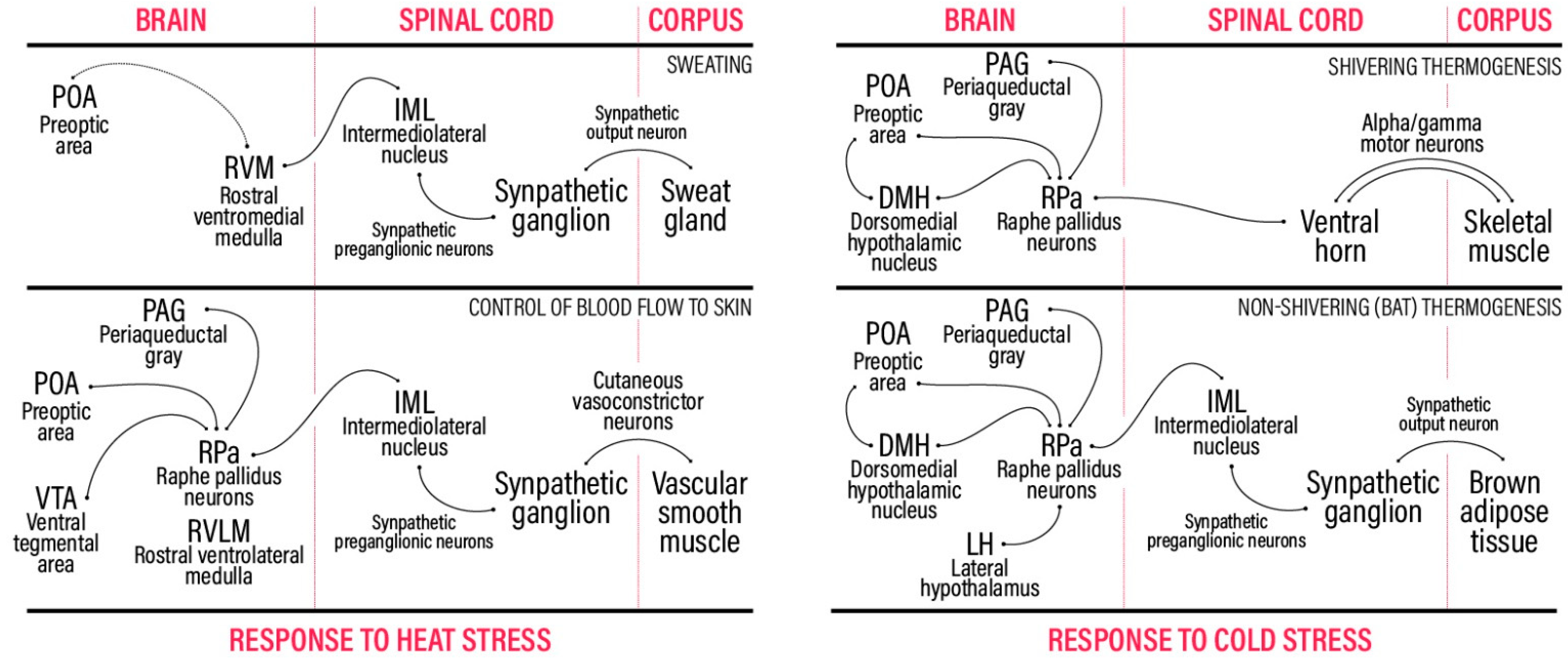
The thermoregulatory physiological responses of the body’s autonomic nervous system mechanisms include regulation of the skin blood flow (vasoconstriction or vasodilation), shivering and sweating (sudomotor activity) [20,21,22]. These physiological functions employ a series of body parts, from outer surfaces to the inner core and, in a sense, compose a layered defence system. This system includes specialised warm and cold thermoreceptor sensors that provide feedback and feedforward to the spinal cord [23], which by their afferent activity drives the relevant regulatory system. An interesting difference between the feedback and feedforward sensing system is that feedback receptors are mainly located throughout the body core, including the brain, viscera and spinal cord and evaluate the internal temperature, while the peripheral receptors on the skin act as feedforward mechanisms by sensing the air temperature around them and anticipate the change in the thermal balance It needs to be noted that there is also a debate whether skin should be classified as a feedforward mechanism. For further discussion, please refer to [24]. Finally, it is worth noting that the stimuli do not always originate from the external sources (i.e., climate), but the body itself might be generating excessive heat due to reasons such as high metabolic rate [25], fighting an infectious or viral disease [26] or regular digestion.
Behavioural adaptation mechanisms can take on a large portion of the thermoregulatory burden, leaving ideally less work for physiological alterations [27,28]. This means that the body is subjected to less stress, and can successfully avoid large internal fluctuations in vital organs [29]. While the stress placed on the body to maintain a stable core temperature is crucial, this does not equal subjecting the human body to a constant ambient temperature. While this may feel “comfortable”, several studies link continuously being in a thermoneutral environment to likeliness of developing obesity, or being susceptible to developing type 2 diabetes [30]. In other words, neither too much stress nor too much comfort is good for human health.
Autonomous thermoregulation is mostly part of the Sympathetic Nervous System (SNS) [31], apart from skeletal muscle shivering, which is controlled by the Central Nervous System (CNS) [32] (see Figure 1).
The skin, while being the largest sensing organ, is also the medium in which first regulation responses happen, i.e., vasomotor or sudomotor activity. This means the skin is also a good indicator to observe the thermoregulation activity in the body. Electrodermal activity (EDA), referring to the changes in electrical conductance of the skin, is a popular biosignal to observe and quantify exocrine sweat activity controlled by eccrine sweat glands [33,34].
However, as the activities of different nervous systems are often overlapping in the domain of the same organ, the sweat secretion on the skin not only indicates SNS activity for thermoregulation but also might mean CNS dictated palmar, mental or emotional sweating [35,36]. A reliable distinction between the two is through the location of measurements in the body: palmar and plantar surfaces, foreheads or axillary and genital regions [37] are linked to psychological sweating response rather than evaporative cooling [38]. For this study, the EDA data is collected through the non-dominant hand’s wrist.
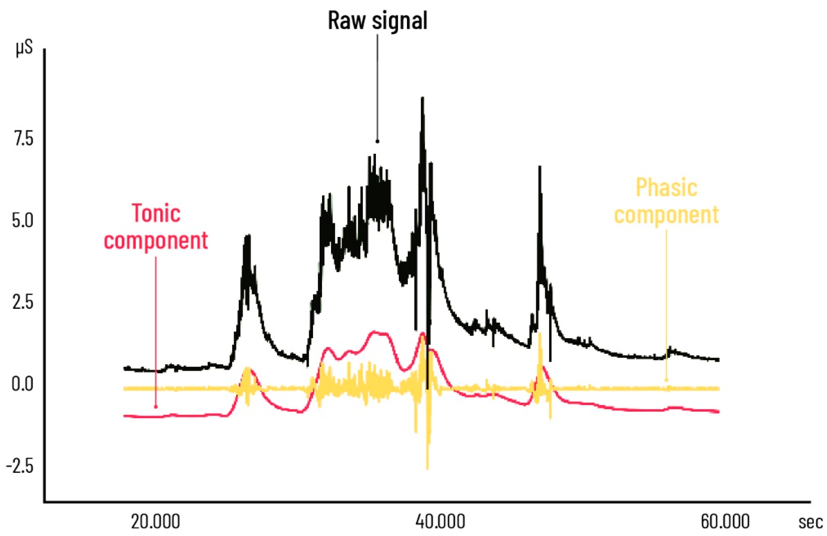
Another fundamental aspect of EDA is its components (Figure 2): The phasic component of EDA reflects the response to a specific stimulus and is generally a fast-changing signal. Skin Conductance Responses (SCR) are considered event-related, and their number, frequency and amplitude are some of their important metrics. A SCR is considered significant when it is higher than 0.04 or 0.05 µS [39] while when it is below this threshold is considered non-specific SCR. SCR ranges are typically smaller than those of the Skin Conductance Levels (SCL) (between 2–20 µS according to Cacioppo et al. [34] and up to 2-3 µS according to Braithwaite et al. [40]). In extreme situations, such as sudden inflicted fearful or threatening stimuli, this maximum can go up to 8 µS, however this is found to be very rare [40]. To set the scale for comparison between SCR and SCL, an SCL increase of 2 µS and more in 30 s is considered as an indicator for a hot flush [37].
The tonic component of EDA is the combination of non-specific SCR activity and SCL and reflects the sweat background activity. The tonic component SCL reflects the slow, long-term sweating procedure. The values are reported as between 1–20 µS within a normal range by Geršak [41], 8–20 µS by Sowden & Barrett [42], 2–16 µS by Braithwaite et al. [40] and 1–40 µS by Venables & Christie [43].
The tonic component is not a direct result of specific stimuli, but an accumulation of non-specific events, which makes it more of an interest when looking into everyday life or long-term allostatic load on the body.
3. Experimental Set-Up
The experimental dataset presented in this paper was collected over 6 weeks, from five volunteers. Two of the subjects (participant 2 and 4) had to come in on the 7th week since they each missed one appointment during the original 6-week period. Experiments started on 10 May 2021 and data collection was concluded on 28 June. The experiment took place in Munich, in the Faculty of Architecture of the Technical University of Munich. The experiment was designed and conducted according to the ethical codes of the University.
All five subjects participating in the experiment were healthy individuals, aged between 24 and 37. Prior to the start of the data collection period, each participant was asked to pick one day of the week to join the experiment, and they came in every week the same day so that their respective schedule structures and type of work over the course of 6 weeks would be similar and comparable to their data from other weeks. The participants’ daily schedules were also kept the same and each participant decided when they would like to start and finish the workday, in order to simulate their normal work experience as much as possible. Each participant spent a total of 7 h in the experiment space each day, of which 6 h were (suggested having been) dedicated for working and 1 h for a lunch break. Additional breaks were all considered in the working hours. All participants worked on their personal laptops, on their day-to-day tasks. Table 1 shows further information for each subject.
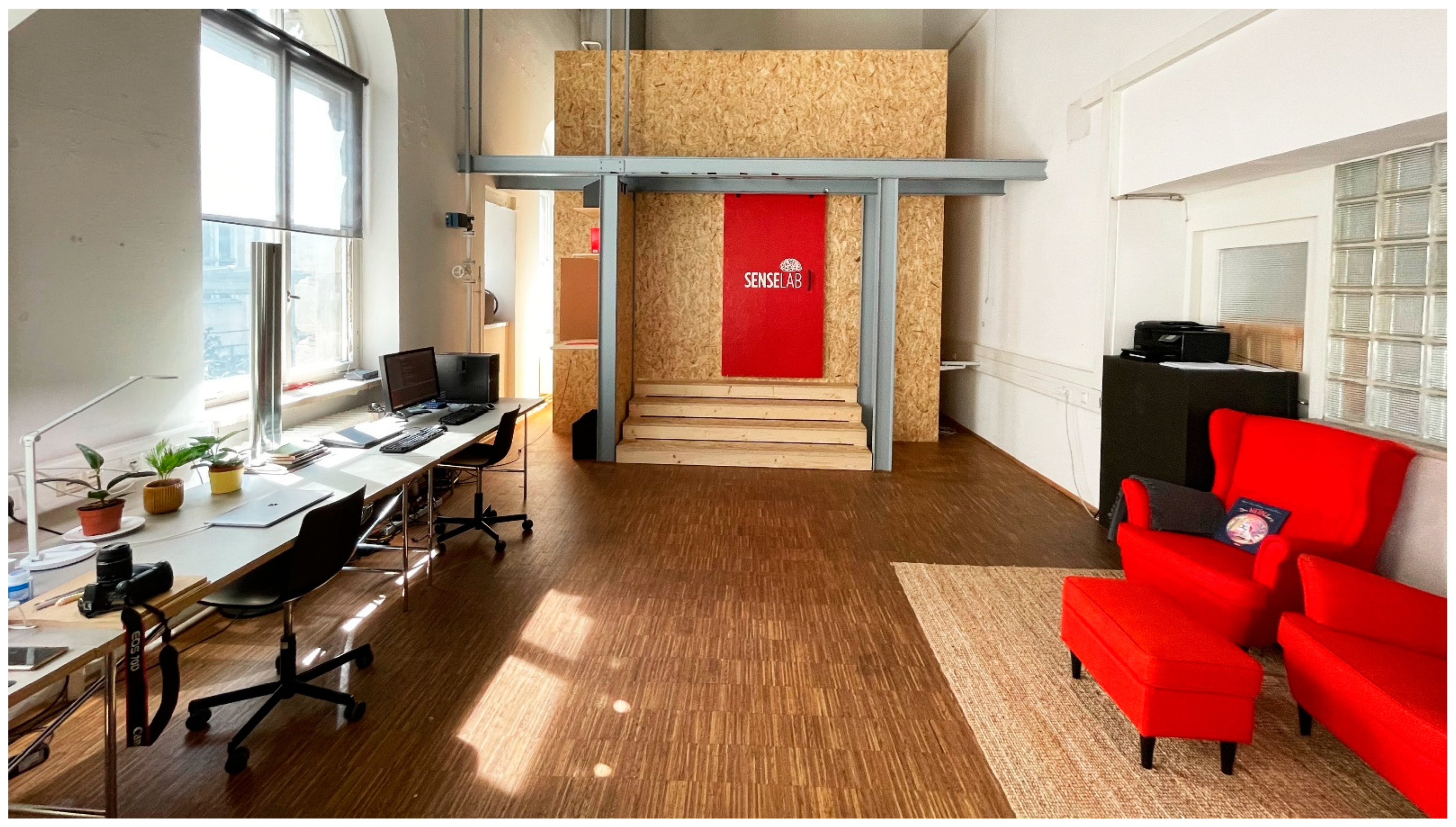
The experiment was carried out in an open plan studio space—Clima Lab. The Clima Lab is a 250 m2, free running space with a ceiling height of 7 m and a façade orientation to the south-east. While the Clima Lab is occasionally used as test space, it functions as a regular open space office containing several desks, a lounge area, a kitchen and a bathroom.
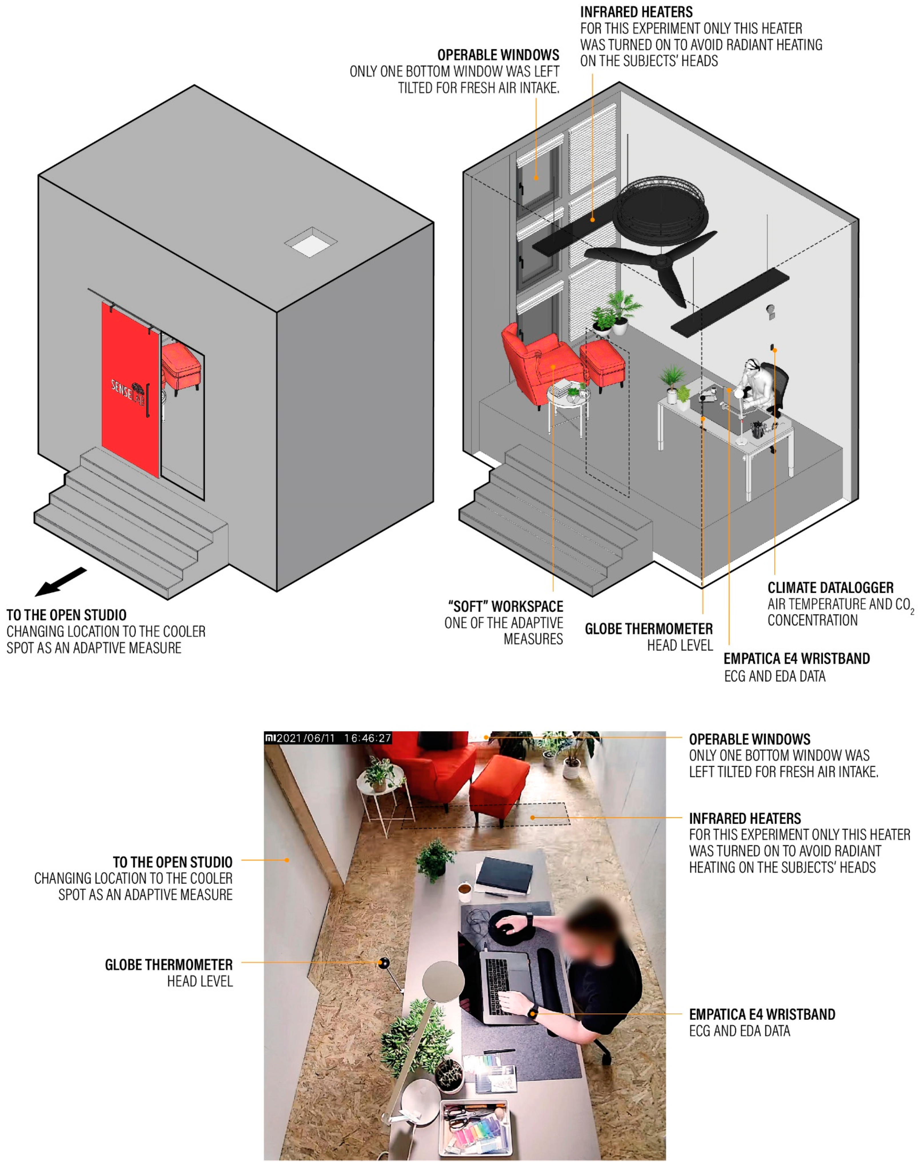
The Sense Lab is a climate chamber within the Clima Lab and located on one end of the space (see Figure 3). Sense Lab is a remotely controllable climate chamber built inside the space. The room surrounding the lab is an actual workspace and is used by a minimum of two (the authors) and a maximum of eight people during the week. The experiment was designed to be in a semi-lab, semi-real-world environment, therefore, the access to the space by other people working there was not restrained.
The open office is not an air-conditioned space during warm seasons, however due to the facade orientation, the urban context and high ceilings the space itself rarely reaches high temperatures. During the data collection, the air temperature inside the open space measured 24.22 ± 1.82 °C, with an overall minus delta of 3.85 ± 2.10 K from the air temperature inside the Sense Lab (see Table 2). The mean radiant temperature inside the Sense Lab was recorded by a globe thermometer placed next to the work desk that the participants have used, on the head level. The temperatures were changed weekly, with no heating the first week, and the data is not used in the analytics. The first week was solely designed to get the test subjects familiarised with the space. The temperature was set to 25 °C (baseline), 27 °C, 28 °C, 29 °C and 30 °C over the course of the remaining 5 weeks, in randomised order. Table 2 shows the temperatures inside the Lab, inside the open studio and outdoors.
The participants were all told that, inside the Sense Lab was their main workstation, however, they were free to take breaks outside the Lab (inside the open office, which was always cooler) whenever they preferred and for however long they needed. Additionally, in order to replicate a realistic scenario, they were allowed to exhibit adaptive behaviour such as changing their clothing and having hot/cold drinks—they were only prevented from any activities that would change the air temperature, such as opening the windows or operating a desk fan. All the adaptive behaviour was marked as they happened. Finally, the participants were told they were free to make changes in the interior layout of the Lab as well as the organisation of the desk—the changes they made were recorded, and the space was transformed according to their personal preferences at the beginning of each day prior to their arrival.
While the globe thermometer temperature for the Sense Lab and air temperature for the open office space was continuously being recorded, each participant was wearing smart monitoring wristbands, on their non-dominant hands to acquire their biometric data. In this study, E4 wristbands from Empatica were used. An extensive study by [44] looks into the reliability of Empatica E4 wristbands, comparing data retrieved from a sample of 345 recordings both by the wristbands and VU-AMS, the “gold standard” tool with established reliability and validity; and comes to the conclusion that, “under non-movement conditions, they propose practical and valid tool for research on HR and HRV”. Table 3 shows the types and respective resolutions of the recorded data.
A typical day started with the test subject arriving to the studio space with their personal laptops. In order to acclimatise their bodies and have them psychologically adapt to the space, a 20 min resting period in the resting area in the studio space is practised. When the subjects settle in this area, the wristbands were put on and recording started. After the resting period, they were asked to enter the Sense Lab and their workday started.
As previously explained, all subjects were told they were free to leave the Lab and take breaks in the “cooler area” as they needed. In line with the hypothesis of the experiment, the breaks were then used as indicators of exceeding the threshold of accumulated thermal stress in the body. The biosignals collected throughout each day was then clustered based on the subjects’ location. The limits of heat exposure, tolerance and physical endurance were examined by looking at the duration of the breaks, recovery time of the body after each break, sensitivity to thermal input after the breaks, effects of adaptive behaviour on tolerance of exposure.
4. Data Analysis and Findings
The data that was collected through wristbands, climate sensors and manual entries on test subjects’ behaviour were all matched by timestamps.
4.1. Overall Observations
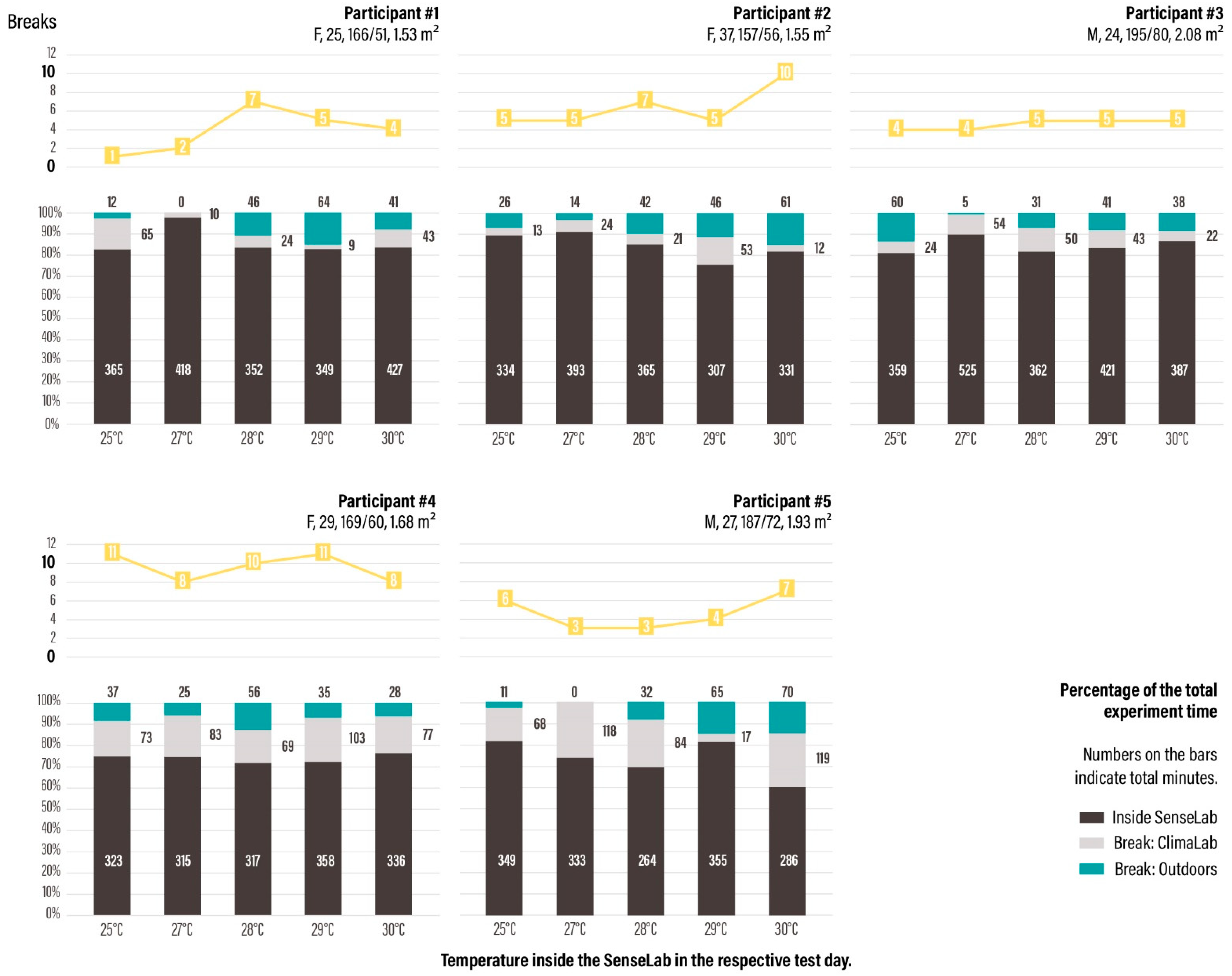
As per the setup of the experiment, it was expected of the test subjects to use the change of space as the initial tool of adaptation. Figure 4 below show the total duration of work inside the climate chamber (Sense Lab), breaks in the cool room and breaks on the outside of the facilities.
As it can be easily observed, there are no clear correlations between the temperature rise and duration/amount of breaks, which rejects the initial hypothesis of spatial adaptation. The authors explain this by means of psychological aspects; even though the test subjects were introduced to the facilities before the experiment started, and an entire first week was used solely to get the subjects used to the space (the data at the end was left out of the resulting dataset), there was still probably no sense of ownership of the space, routine, set expectations, familiarity/relationship with other people in the shared office (cool room), or so. This, in theory, most likely limited the free use of all available spaces and the subjects might have preferred to stay in the climate chamber longer, albeit the heat stress. The effect of similar psychological decision-making on heat tolerance is an aspect to be studied in the future.
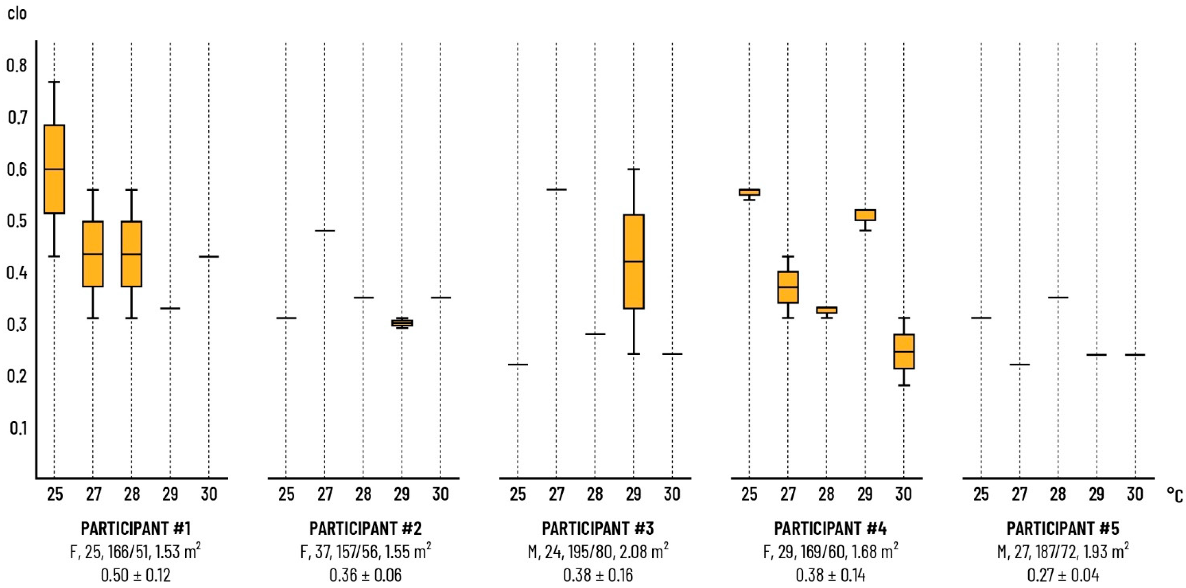
As for the other adaptive behaviour, change of the clothing was also constantly observed and marked. Figure 5 shows the variation of clothing values per participants, for each test day. Similar to the break pattern, there is no clear trend between the rise of the temperature and clothing decision. However, similar to the number of breaks taken during the day, the number of clothing changes presents a different characteristic behaviour for each participant.
4.2. Physiological Response
This study focuses on the investigation of EDA activity in different ambient temperature environments. The raw EDA signals had a sampling frequency of 4 Hz and were analysed using the Neurokit2 library for Python [49], i.e., filtered, cleaned, and then divided into phasic (SCR) and tonic (SCL) activities, while the SCR peaks were identified.
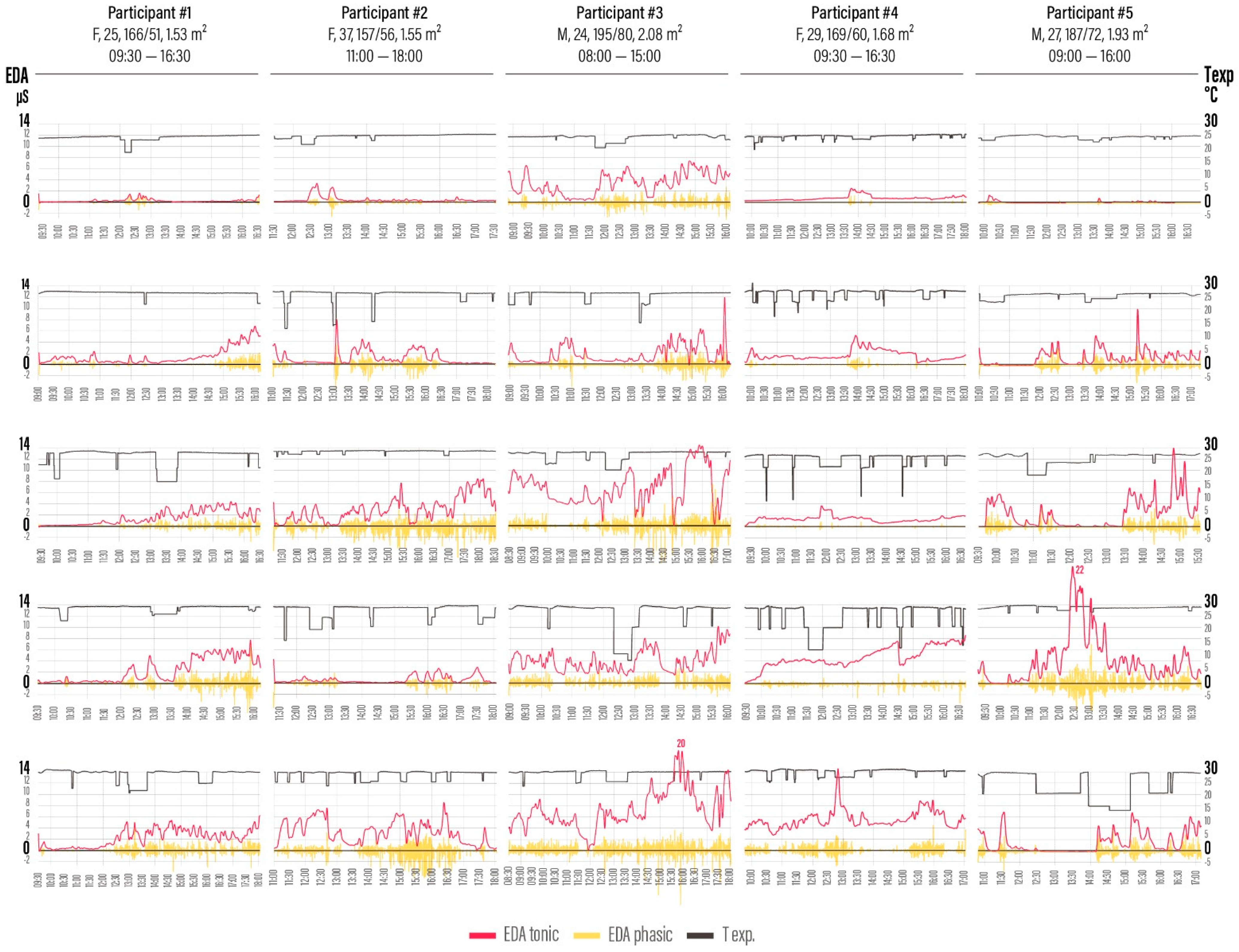
Below (Figure 6) are the graphs illustrating The EDA levels of each test subject from different days, against the temperature that the subjects were exposed to at the respective time.
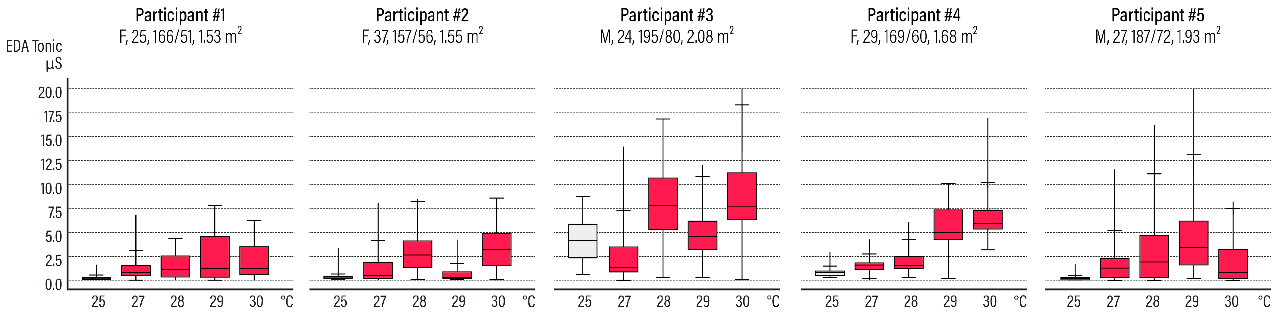
As mentioned previously, the main part of the data analyses focused on tonic component. The 25 °C day was accepted as the baseline for all participants. As expected, generally the EDA activity is at its minimum for all—however a comparison between Participant 3 and others clearly show the difficulty in making inter-person analysis with absolute numbers. As a clear example, while Participant 3 had a tonic range of 0—7.5 µS during the 25 °C day, this is the maximum range ever observed for Participant 1, including the 30 °C day (see Figure 7). This has been found previously in literature as “within-subjects correlations being much higher than those between-subjects” [36,37,48].
The tonic EDA is a slow varying signal over time, thus for each participant/session, a sliding temporal window of ∆t = 1 min and step of 1 min was used after carefully checking that does not affect the information and the signals’ variability.
As EDA presents inter-subject variability, it is appropriate to take into account each participant’s personalized EDA tonic baseline (grand average of 25 °C). The differential to baseline EDA tonic values were extracted generating a common reference for EDA across subjects providing data normalization.
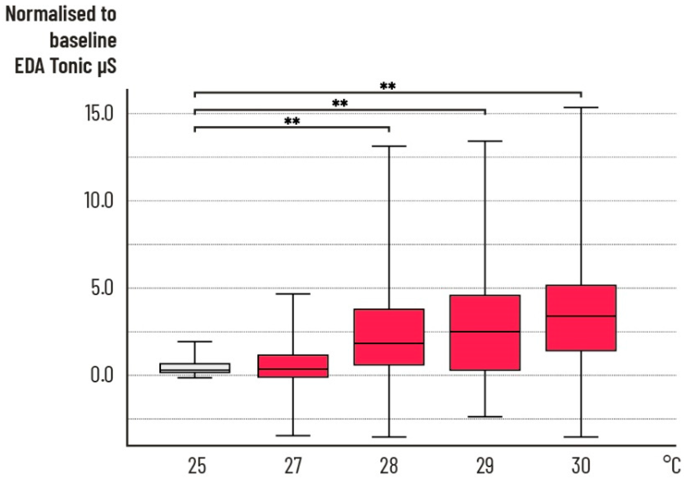
The normalized data elicited statistically significant changes in normalized tonic EDA over temperature (Kruskal-Wallis H test, H(4) = 5335.45, p < 0.001). Pairwise post-hoc analysis with Bonferroni correction on multiple comparisons revealed statistically significant differences in median tonic EDA values between 25 °C and 28 °C (p < 0.001), 25 °C and 29 °C (p < 0.001) and 25 °C and 30 °C (p < 0.001). The results are presented in Figure 8.
It can be observed from Figure 8, that tonic EDA presents a statistically significant increase after the 28 °C and above this temperature (i.e., 29 °C and 30 °C). Although there are several studies that compare EDA levels under different temperature settings, to the authors’ best knowledge, there are no comparable datasets that collected EDA data under the same temperatures and temperature steps. In the occupational health, psychophysiology or biomedical studies where the use of EDA has been traditionally more common, either the ambient temperature was kept to the thermoneutral ranges (22–26 °C depending on the study [37]) or where the impact of ambient temperature was studied, bigger steps of temperature changes were tested [50,51]. Therefore, the observed finding could not be compared to the existing literature. However, the clear difference of change in means from 27 °C to 28 °C will be observed with further data collection.
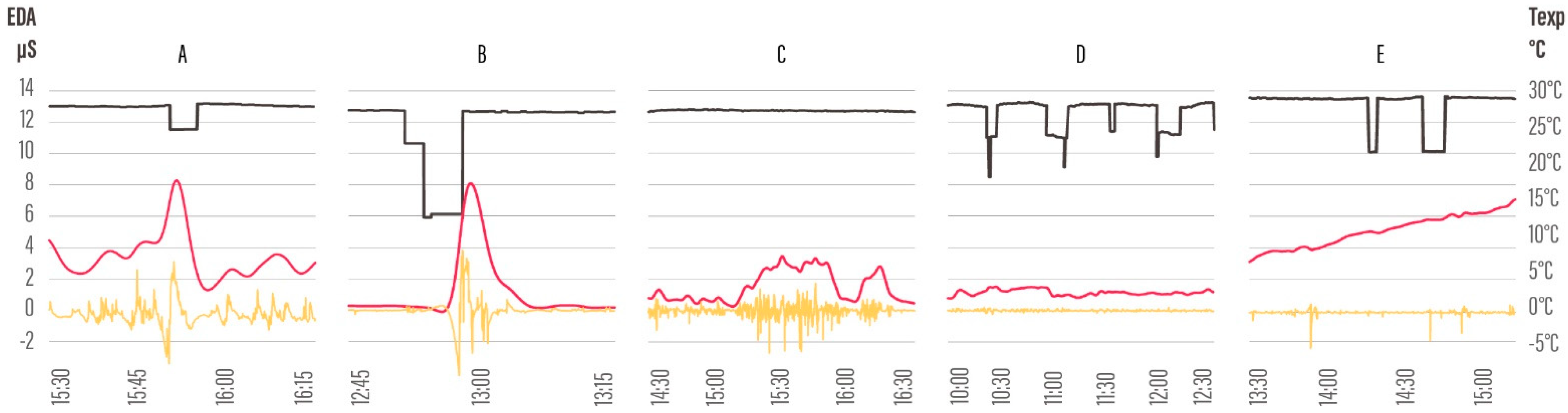
Additionally, even though statistical analyses present significant relevancy, it must be noted that when looked in detail, there are several moments where there are contradicting relationships between tonic EDA and temperature trends. Figure 9 shows some of these moments. In the future studies, such inconsistencies should be examined carefully and eliminated and/or normalized wherever needed.
4.3. Temporal Change
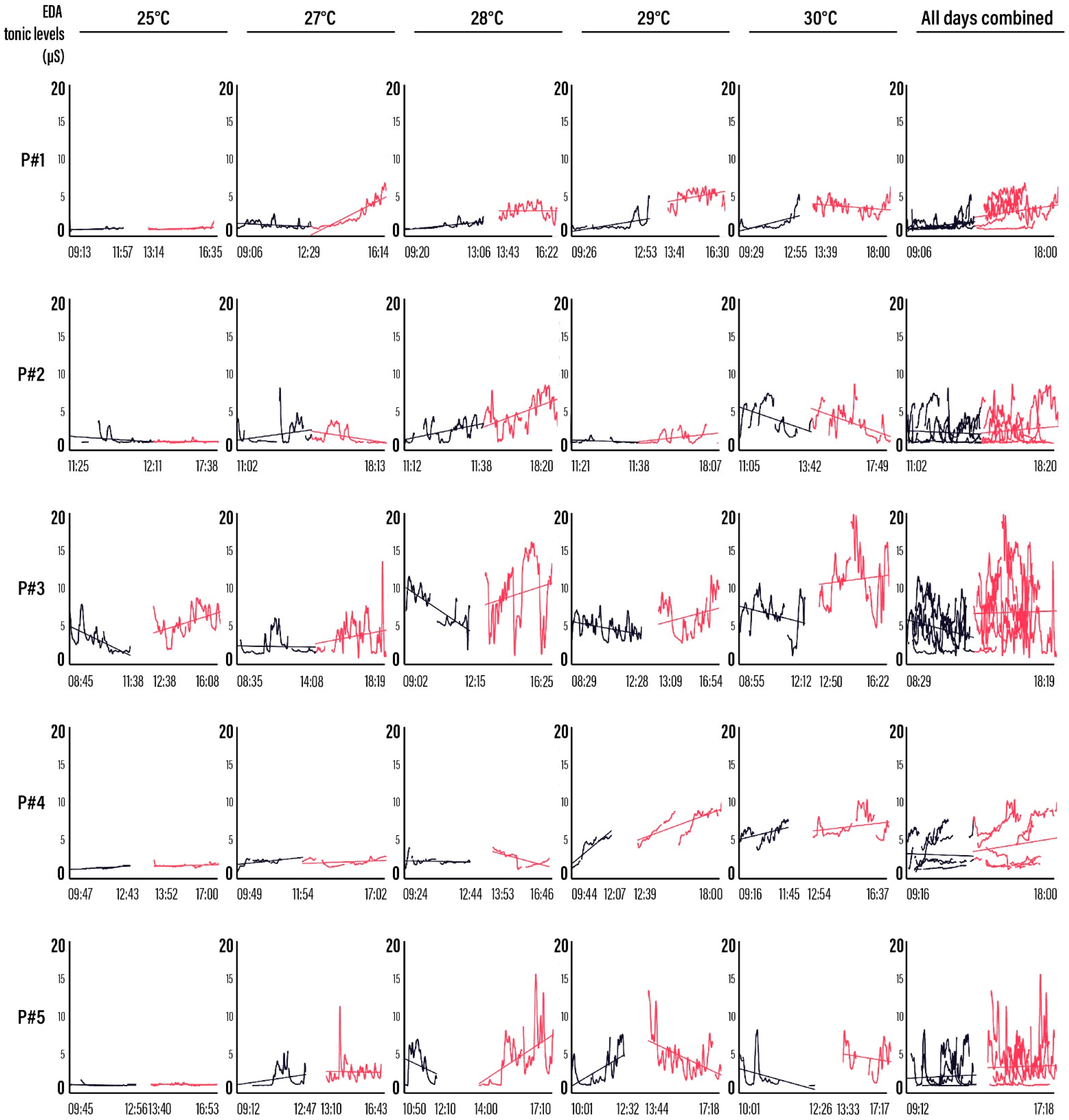
Another visible observation was the change of physiological reaction to similar conditions over time within the same day. As speculated beforehand, this study is not only interested in how different spaces with different thermal setups affect the human body, but also when and for how long. In that regard, the same SCL data was plotted against time. A k-means clustering (elbow joint at k = 2) revealed a change in regression around lunchtime in most of the cases (see Figure 10). It must be noted that in all of the following analyses, the dataset is only for when the participants were inside the Sense Lab. Therefore, the gaps in the timelines show the breaks.
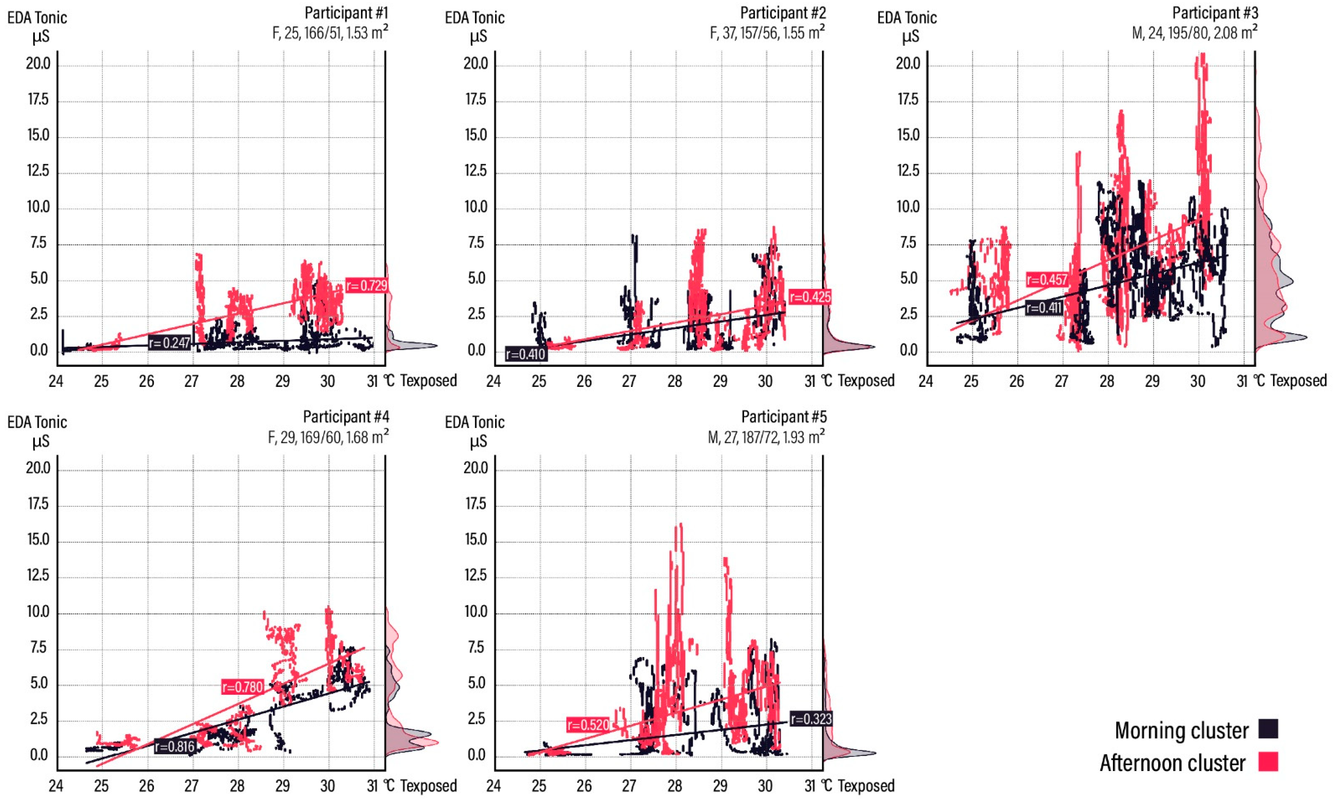
Scatter plots with temperature and SCL values illustrate the overall effect (Figure 11). The differences in morning and afternoon clusters are clearly visible in some participants (Participants 1 and 5), more moderate in some others (Participants 3 and 4), and an insignificant difference can be seen in one (Participant 2).
The correlation of the tonic EDA values with temperature of all participants was checked for morning and afternoon cluster. The correlation of the EDA and temperature was greater for the afternoon cluster (r = 0.449, p < 0.001) in relation to the morning cluster (r = 0.332, p < 0.001). The statistical significance of the morning and afternoon correlation was checked using the Williams’s Test [52]. The data were transformed according to the Fischer transformation
in order to be normally distributed. The statistic z of the test is given by the formula
where r1, r2 are the correlation coefficients between EDA and temperature of the morning and evening cluster, respectively, and n1, n2 are the samples of the morning and evening cluster, respectively.
The William’s Test resulted in statistically significant higher correlation between tonic EDA and temperature in the afternoon cluster (z = 6.534, p < 0.001) in relation to the morning cluster.
At first glance, there were several possible explanations for the differences in “morning” and “afternoon” clusters:
1. The participants left the climate chamber for lunch, walked to a nearby restaurant (less than 10 min) and walked back. This rise in activity level, especially after having the entire morning spent sitting in front of a desk, might have resulted in higher EDA overall.
However, on two separate occasions, the participants did not even leave the space for lunch and decided to sustain on smaller snacks throughout the day, not walking for longer than the distance to the bathroom. The clusters were very similar. Additionally, while the majority of participants had their cluster divisions very close to lunch breaks (for these four participants, “afternoon” cluster starts 00:08 ± 00:14 after the lunch break) Participant 2, who started her day an average 2 h later than the other participants, has her cluster division time 01:23 ± 01:18 after her lunch break. And finally, for Participant 3, on the days of 27 °C and 28 °C tests, the division starts an hour before the lunch break ends (see Table 4).
2. The digestion of lunch could have raised the metabolic rate and the body temperature. The explanation of the above exceptions apply in this case as well.
3. The EDA was affected by the circadian rhythm of the body and with the natural rise in body temperature in the afternoon, the skin was less capable of handling heat and started accumulating stress, which was also the reason of the higher correlation between temperature and EDA levels in the afternoon. The rise in the tonic EDA is less impacted by the rise in temperature in the morning clusters, hence the lower correlation.
Note that most participants (1, 3, 4 and 5) had starting times between 8.15–9.30, while Participant 2 started at 11.00 by her own choice. Her clustering places not so differently from others, with nearly 3.5 h after her starting time. This raises the question whether her natural circadian rhythm has shifted accordingly, or the main determinant is the amount of time spent in the Sense Lab, or a balance of the two.
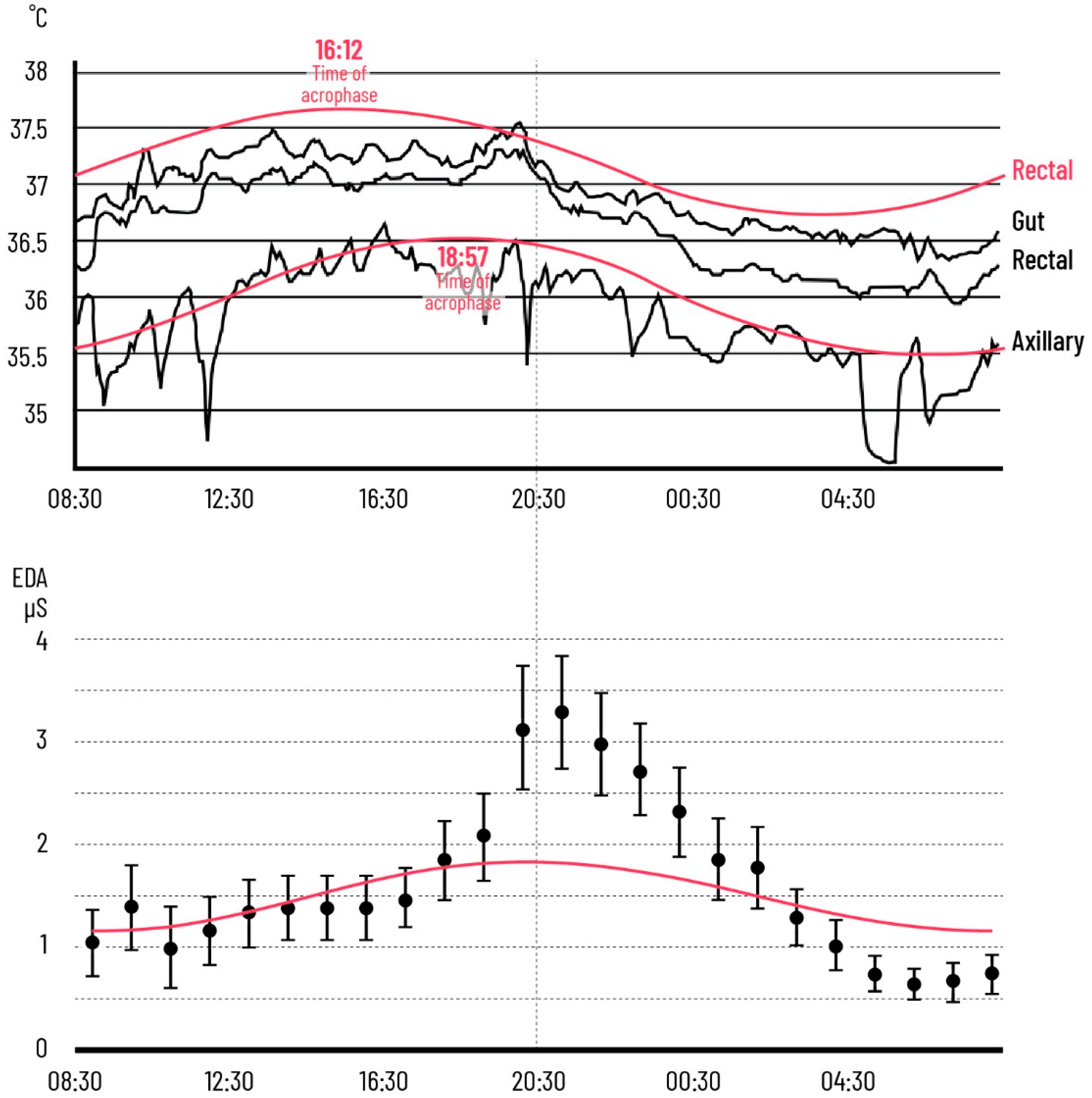
The daily oscillation of the body temperature over the full 24 h cycle is nearly 1 °C [53], and can be even higher based on gender, age and other factors. The temperature is at its lowest in the morning (bathyphase), and highest in the afternoon (acrophase), mirroring the Midline Estimating Statistic of Rhythm (MESOR) line. While for a person that is awake between 7:00 and 23:00 o’clock, the bathyphase is between 03:00 and 06:00 o’clock, and the acrophase is observed between 18:00 and 21:00 o’clock, a more universal rule of thumb can be generalised as the acrophase happening 12 h after waking [54].
In a recent research, Kim et al. [55] ran a 2-day long study in a hospital environment with 14 healthy adults, and found that EDA showed significant similarity to the circadian rhythm, by differing from mean value by 15% around 16:00 o’clock. This correlation and its implications need further exploring, however such a temporal clustering of the relationship of the human and its environment can be a promising start in handling the spaces more efficiently and sufficiently. Another study from 2021 by Vieluf et al. [56] collect data from 119 patients and model the EDA level curve over the 24 h period, with an oscillation of 2 µS in the individual means, and around 0.3 µS in the best fitting pattern (Figure 12).
4.4. Same Analyses with PMV
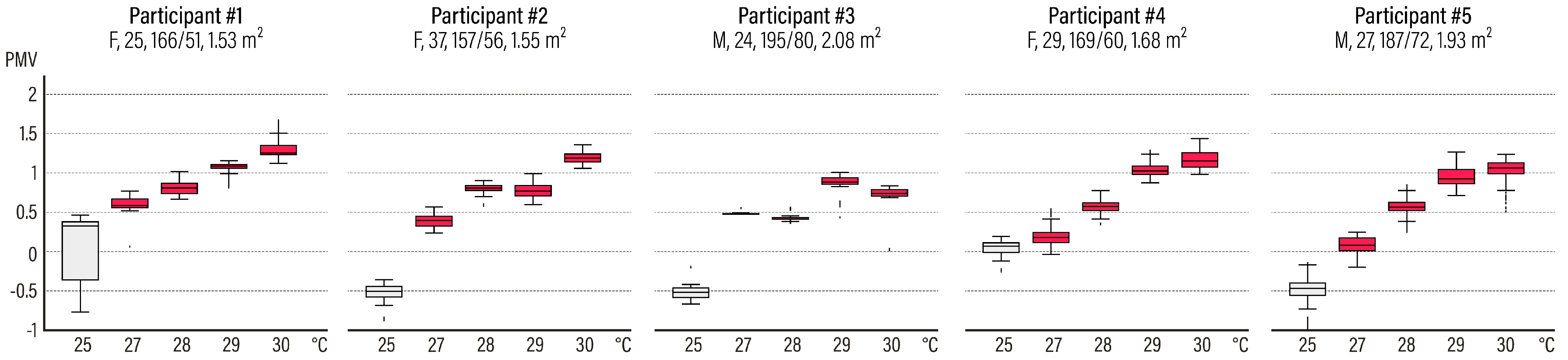
Until now the physiological data was compared against operative temperature. However, this naturally does not reflect the other elements of heat-balance models, or the impact of the adaptive behaviour. In this section, PMV and PPD values were calculated based on the clo values that were observed and recorded throughout the experiments and relative humidity values measured by the climate logger. Throughout the experiment, the relative humidity inside the Sense Lab during occupied time ranged between 20.18% and 46.41% (mean ± STD is 31.67 ± 7.5%). The metabolic rate was fixed at 1.1 met for light work on computer, and the air velocity was assumed as 0.05 m/s since the Sense Lab is entirely isolated from the outside and the windows at the façade were kept closed during the experiment. The PMV and PPD calculations were done using pythermalcomfort library [59] on Python. Figure 13 shows the PMV ranges for each participant, in respective test days.
Since air velocity and metabolic rate was set to a constant and operative temperature was kept in a tight range (see Table 2), parameters affecting the PMV were relative humidity and clo values. The variation in RH was quite low throughout the data collection period therefore suggesting that changes in the clothing values affecting the PMV ranges.
The joint effect of temperature and humidity on PMV was investigated using a partial least-squares linear regression model [60]. The model was fitted to the temperature, humidity parameters estimating the involvement of each parameter in the regressive response outcome PMVregr,
where β0 is the intercept, β1, β2 are the model coefficients of temperature, humidity respectively and e is the residual (unexplained variance in PMVregr). The regressive response outcome PMVregr contains the combined involvement of temperature and humidity on PMV. The regression model parameters were estimated as,
For estimating the significance, the regression model was fitted on each participant in a sliding window of 60 s and step of 60 s. Due to the highly correlated time series, the subject’s p-value was adjusted by dividing by the number of samples. The total combined p-value was estimated as the mean values of the individual p-values leading to a p < 0.001 for temperature and a p = 0.04 for humidity. Therefore, the temperature was the most significant parameter affecting positively PMV following by humidity which has a marginal significant negative effect.
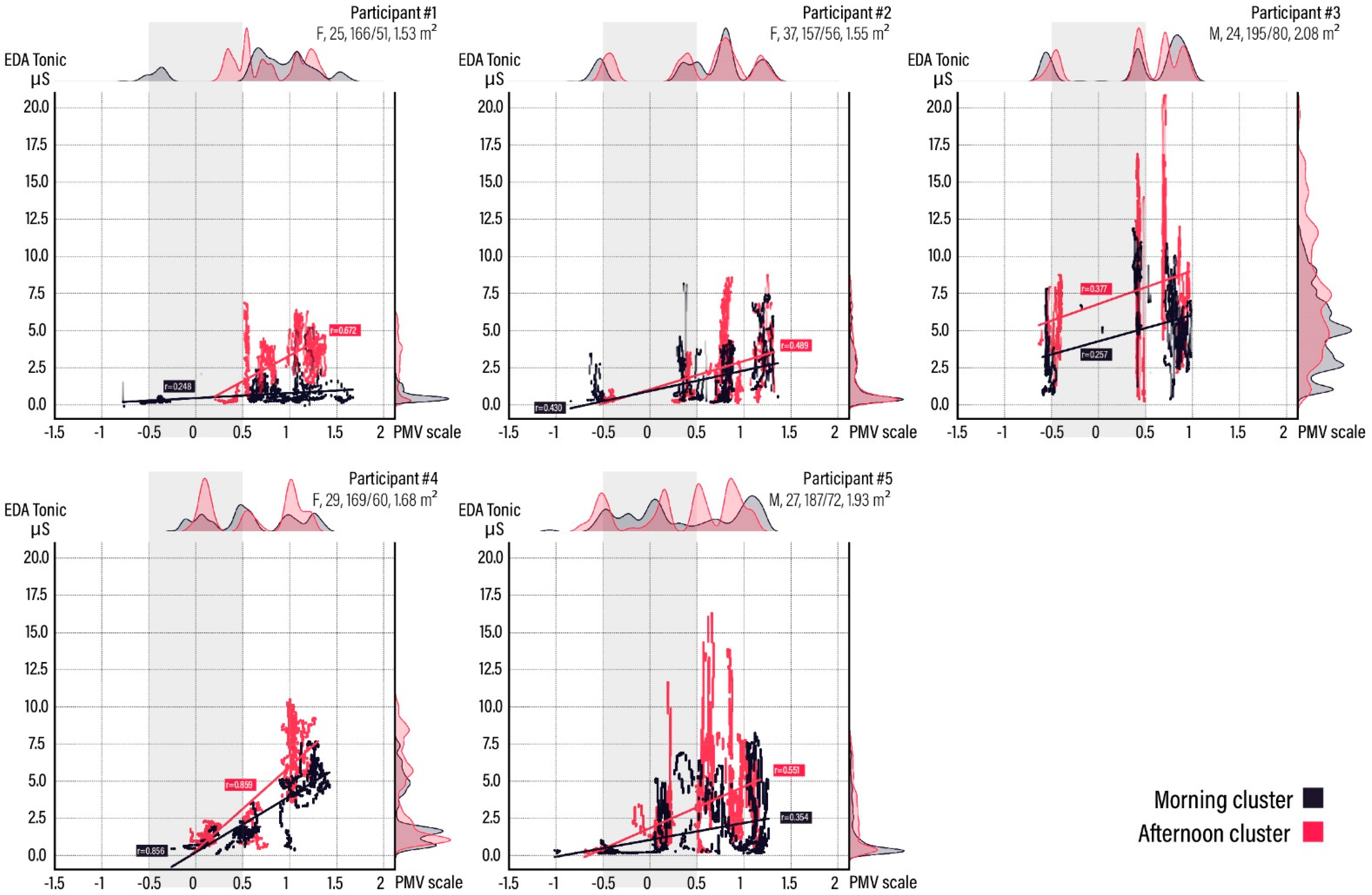
The results (Figure 14) therefore, do not show a significant difference in findings in comparison to the previous plots with temperature (Figure 11) as expected. When compared, afternoon and morning clusters present a larger range of tonic values for the same PMV value, similarly to the operative temperature.
5. Limitations and Discussion
The first point of discussion is the minimal personal comfort perception/satisfaction feedback against the biometric datasets. Collecting both quantitative and qualitative data and attempting to correlate them is a common practice in similar studies, and believed to offer further insight when coupled with objective data [61,62]. However, in the experiment presented in this paper, elimination of any kind of survey-like feedback was intentional. Thermal comfort is, in reality, the lack of discomfort, or more precisely and bypassing the double negatives, it is neutrality [63]. Some studies reveal that these questionnaires, however short, easy or presented with well-designed user interfaces, still pose a threat for bias or show problems with reproducibility [64,65,66,67,68,69]. While the comparison between physiological data and psychological feedback is worth investigating, the authors decided to collect the subjective feedback only through the event-mark buttons, when the sensation would be defined as “thermally stressful” by the participants. No grading or further questioning was required, the only metric considered was the time the participants remembered to press a button that they were only reminded of in the beginning of the experiment. This event-mark button, however, was rarely used by the participants even in the highest temperature days, and therefore its data was excluded in the publication.
Due to the nature of the research questions at hand, the design of the experiment intended to replicate a real-world setting as much as possible. By doing so, the participants were given all the flexibilities and adaptation options as a regular workspace with adaptive capabilities would normally have. However, the use of windows and additional fans were prohibited in order to keep a stable temperature inside the test space—which can be argued as a significant psychological setback.
Furthermore, even though the first week of data collection was intended for the test subject to familiarise with the space, lockers were provided for the subjects to bring and leave their belongings, and the authors observed and re-created individual preferences in the Sense Lab for each person at the beginning of their test-day (i.e., the choice of work chair, desired items on the desk, etc.); the authors speculate that it still may not be enough time to simulate a realistic tolerance behaviour that the subjects would exhibit in “their own” workspaces, as they only used the space six times over the span of 6 weeks and formed no routines. Furthermore, while they were informed that the temperature inside the Sense Lab might be different during different days, and despite having alternative clothing in their lockers, the lack of anticipation and expectation, most likely limited any gradual acceptance of the high temperature. At the end, the observed behaviour throughout the experiment period left the authors unsure about whether the employed strategies to make the participants feel “at home” worked. It is worth mentioning that, the upcoming experiment designs need to be more conscious of the Hawthorne effect and find ways of overcoming it [70,71].
Additionally, while the age range of the participants is not limited to those of the typical student age group, it can be argued that it is still not fully representative of people that are expected to work in office environments. A sample group of five people does not constitute as representative either. However, the findings in this paper are presented as preliminary and will be treated as a basis for future research. The experiment is replicable with different and more participants.
In addition to the missing psychological parameters, some physiological aspects were also ignored within this study: On the hottest days when temperatures in the Sense Lab were 29 °C or 30 °C, some of the participants (1, 2 and 5) verbally mentioned that they felt that they were getting tired faster, relative to lower temperatures, when working inside the Lab. While several studies have been looking into the relationship between thermal stress and cognitive workload [72,73,74,75,76], this component has been left out from the experiments for now. Nevertheless, the impact of thermal variations on cognitive workload is an aspect that the authors will be examining in the upcoming experiment series.
6. Conclusions
The experiment collected data of five participants over the course of 6 weeks. The resulting datasets included climate, physiologic and behavioural data with varying resolution and finally matched time-wise. The analysis focused on the relationship between tonic EDA to understand the impact of the thermal stimuli on the human body in a varying spatiotemporal setup.
Initial research question at hand was the correlation between time and thermal exposure. The data suggested that there was a difference in tonic EDA levels between “morning” and “afternoon” clusters although the environmental parameters were the same, suggesting a change in the human body’s thermal reception over time. Even further, based on the person’s chronotype, the beginning of the “afternoon” cluster was observed to have shifted according to the person’s circadian rhythm. Such individual shifts have been remarked in the literature previously [77], and there are several studies that present data on the changes in the core temperature and on the skin conductance throughout the day [55,56,57,58]. Understanding this phenomenon in the context of design and operation of the built environment might reveal opportunities in a change in office schedule-culture, which could mean lowering and balancing the energy demand throughout the day, while actually offering a healthier life-style for people as well.
Second research question was whether taking cool breaks would help with such accumulation of stress in the body, and if so, whether a “reset” time could have been identified. However, the use of breaks as an adaptive behaviour did not take place as expected and the data did not yield clear trend. The authors intend to conduct further experiments to investigate this relationship again in the future, this time with controlled schedules.
Finally, an underlying question was comparing health to comfort. As discussed previously, only focusing on one physiological output is not representative of the body’s health panel but a mere scratch on the surface. However, initial comparisons reveal how the body reacts differently under the same PMV values, both within and between-subjects.
At the moment no conclusion could be driven through the presented EDA data of any of the participants as to say what is “healthy” or “not healthy”. This is for several reasons:
1. As previously explained the absolute numbers do not reveal much and the evaluation should be done within-subject. Further longitudinal studies need to collect more data from individuals to identify trends of within-subject changes.
2. While electrodermal activity was paralleled to a higher/lower sympathetic nervous system (SNS) activity, without cardiovascular activity a complete argument should not be made. The dermal related thermoregulation activities, as previously mentioned, employ vasomotor responses, which is directly connected to the blood flow. In order to dissipate more heat, the heart needs to direct a larger portion of blood circulation to skin, in some cases as much as 60% [78]. Management of these sudden peaks and blood pressure regulation is a health-critical SNS over-activity example. Therefore even though EDA levels are indicative of SNS load, cardiovascular data should be studied in parallel.
3. Another important aspect is mental workload: with the blood redirection from organs to skin in order to achieve thermal homeostasis, cerebral blood flow is also impaired. Even a seemingly small rise of 0.3°K in core temperature (esophageal) with a rise of 3.8°K in skin temperature is found to cause a 15% decrease in blood flow in middle cerebral artillery flow [79]. While measuring the blood flow in brain systems may not be suitable in experiments designed in a climate chamber, the cognitive workload as a result of it may still be observed and measured via mobile EEG headsets.
7. Further Research
The analyses presented in this paper consists of 150 h of data collected from five subjects. As pointed out in Limitations and Discussions, while the within-subject data size is bigger than studies of similar research, number of participants are not adequate to derive conclusions. However, the entire study and the set-up of the climate chamber is so that the same data collection is to be repeated in a way that comparable data under the same conditions will be produced. The authors are planning to continue to expand the dataset and will re-evaluate the initial findings that were presented in this paper.
Another aspect that was mentioned previously, the additional biosignals (i.e., cardiovasciular and EEG data) are to be included in the same analyses, not only to search for similar patterns that were found in this paper, but also to look for inter-biosignal correlations.
Finally, in the long-stretch, this research and accumulated comparable psychophysiological data collected in similar controlled experiments will be used to design a new model that is inclusive of the effect of time, and based on objective parameters that also point to the health implications of the built environment.
In this age of long-waited mindfulness for the environment, the building professionals should shift their views towards the active systems: their existence must simply be justified as an absolute necessity, rather than being accepted as the norm. As Addington and Schodek state, “(o)nly the human body requires management of its thermal environment, the building does not.” [80]. Understanding the physiological response in a higher resolution might enable us to design spaces and their operation in a similarly higher resolution not only in space but also in time. Revealing time and space-dependent correlation between the temperature and human body’s reception and processing of it can help the building professionals treat the spaces in smaller units with different time schedules—which might help us come closer to the sufficiency that we need. The comfort models have all relied on extensive data collection and repeated experiments with different variables. Similarly, we need to make use of the new tools available to us, as quantifying the psychophysiological behaviour would be a valuable addition to the existing global databases on comfort.
Author Contributions
Conceptualization, B.K. and S.C.K.; Methodology, B.K., S.C.K. and G.G.; Formal analysis, B.K. and G.G.; Investigation, B.K., K.N. and G.G.; Data curation, B.K. and G.G.; Writing—original draft, B.K., S.C.K. and G.G.; Writing—review & editing, B.K., S.C.K. and G.G.; Visualization, B.K. and G.G.; Supervision, B.K. and T.A.; Project administration, B.K. and S.C.K. All authors have read and agreed to the published version of the manuscript.
Funding
This research was funded through contributions of the TUM SEED FUND RESEARCH through a research grant to Bilge Kobas.
Institutional Review Board Statement
The study was conducted according to the guidelines of the Technical University of Munich. All participants signed informed consent. Starting from the data acquisition, the authors did not keep any data that could identify the participants, and the datasets were constructed as completely anonymous. Therefore, ethical review and approval were waived for this study.
Informed Consent Statement
Informed consent was obtained from all subjects involved in the study.
Data Availability Statement
The data is not yet publicly available, however upon request from the corresponding author, can be shared.
Acknowledgments
The authors would like to extend their gratitudes to the participants of the experiment.
Conflicts of Interest
The authors declare no conflict of interest. The funders had no role in the design of the study; in the collection, analyses, or interpretation of data; in the writing of the manuscript, or in the decision to publish the results.
References
- Fanger, P.O. Thermal Comfort; Technical University of Denmark, Laboratory of Heating and Air Conditioning; Danish Technical Press: Copenhagen, Denmark, 1970. [Google Scholar]
- Gagge, A.P.; Fobelets, A.P.; Berglund, L.G. A Standard Predictive Index of Human Reponse to Thermal Enviroment. Am. Soc. Heat. Refrig. Air-Cond. Eng. 1986, 92, 709–731. [Google Scholar]
- Nicol, J.F.; Humphreys, M.A. Thermal Comfort As Part of a Self-Regulating System. Build Res Prac. 1973, 1, 174–179. [Google Scholar] [CrossRef]
- de Dear, R.; Brager, G. Developing an Adaptive Model of Thermal Comfort and Preference. ASHRAE Trans. 1998, 104, 145–167. [Google Scholar]
- de Dear, R.; Zhang, F. Dynamic Environment, Adaptive Comfort, and Cognitive Performance. In Proceedings of the 7th International Buildings Physics Conference, IBPC2018, Syracuse, NY, USA, 23–26 September 2018; pp. 1–6. [Google Scholar]
- Zhang, H.; Huizenga, C.; Arenas, E.; Wang, D. Thermal Sensation and Comfort in Transient Non-Uniform Thermal Environments. Eur. J. Appl. Physiol. 2004, 92, 728–733. [Google Scholar] [CrossRef]
- Warthmann, A.; Wölki, D.; Metzmacher, H.; van Treeck, C. Personal Climatization Systems-a Review on Existing and Upcoming Concepts. Appl. Sci. 2018, 9, 35. [Google Scholar] [CrossRef] [Green Version]
- van Marken Lichtenbelt, W.; Hanssen, M.; Pallubinsky, H.; Kingma, B.; Schellen, L. Healthy Excursions Outside the Thermal Comfort Zone. Build. Res. Inf. 2017, 45, 819–827. [Google Scholar] [CrossRef] [Green Version]
- Leaman, A.; Baordass, B. Building Design, Complexity and Manageability. Facilities 1993, 11, 11–27. [Google Scholar] [CrossRef] [Green Version]
- Schützenhofer, C. Overcoming the Efficiency Gap: Energy Management as a Means for Overcoming Barriers to Energy Efficiency, Empirical Support in the Case of Austrian Large Firms. Energy Effic. 2021, 14. [Google Scholar] [CrossRef]
- Kolarik, J.; Toftum, J.; Olesen, B.W.; Jensen, K.L. Simulation of Energy Use, Human Thermal Comfort and Office Work Performance in Buildings with Moderately Drifting Operative Temperatures. Energy Build. 2011, 43, 2988–2997. [Google Scholar] [CrossRef] [Green Version]
- Parkinson, T.; De Dear, R.; Candido, C. Thermal Pleasure in Built Environments: Alliesthesia in Different Thermoregulatory Zones. Build. Res. Inf. 2016, 44, 20–33. [Google Scholar] [CrossRef]
- Ryu, J.; Kim, J.; Hong, W.; de Dear, R. On the Temporal Dimension of Adaptive Thermal Comfort Mechanisms in Residential Buildings. IOP Conf. Ser. Mater. Sci. Eng. 2019, 609, 042071. [Google Scholar] [CrossRef] [Green Version]
- Pitoni, S.; Sinclair, H.L.; Andrews, P.J.D. Aspects of Thermoregulation Physiology. Curr. Opin. Crit. Care 2011, 17, 115–121. [Google Scholar] [CrossRef]
- Lopez, M.; Sessler, D.I.; Walter, K.; Emerick, T.; Ozaki, M. Rate and Gender Dependence of the Sweating, Vasoconstriction, and Shivering Thresholds in Humans. Anesthesiology 1994, 80, 780–788. [Google Scholar] [CrossRef]
- Tan, C.L.; Knight, Z.A. Regulation of Body Temperature by the Nervous System. Neuron 2018, 98, 31–48. [Google Scholar] [CrossRef]
- Terrien, J. Behavioral Thermoregulation in Mammals: A Review. Front. Biosci. 2011, 16, 1428. [Google Scholar] [CrossRef] [Green Version]
- Nagashima, K. Central Mechanisms for Thermoregulation in a Hot Environment. Ind. Health 2006, 44, 359–367. [Google Scholar] [CrossRef] [PubMed] [Green Version]
- Kingma, B.R.M. The Link between Autonomic and Behavioral Thermoregulation. Temperature 2016, 3, 195–196. [Google Scholar] [CrossRef] [PubMed] [Green Version]
- Kurz, A. Physiology of Thermoregulation. Best Pract. Res. Clin. Anaesthesiol. 2008, 22, 627–644. [Google Scholar] [CrossRef] [PubMed]
- Filingeri, D. Neurophysiology of Skin Thermal Sensations. Compr. Physiol. 2016, 6, 1429. [Google Scholar]
- Bronzino, J.; Enderle, J.; Enderle, J. Introduction to Biomedical Engineering, 3rd ed.; Enderle, J., Bronzino, J., Eds.; Elsevier Inc.: Oxford, UK, 2012; ISBN 978-0-12-374979-6. [Google Scholar]
- Nagashima, K.; Nakai, S.; Tanaka, M.; Kanosue, K. Neuronal Circuitries Involved in Thermoregulation. Auton. Neurosci. Basic Clin. 2000, 85, 18–25. [Google Scholar] [CrossRef]
- Romanovsky, A.A. Skin Temperature: Its Role in Thermoregulation. Acta Physiol. 2014, 210, 498–507. [Google Scholar] [CrossRef]
- Vinkers, C.H.; Penning, R.; Hellhammer, J.; Verster, J.C.; Klaessens, J.H.G.M.; Olivier, B.; Kalkman, C.J. The Effect of Stress on Core and Peripheral Body Temperature in Humans. Stress 2013, 16, 520–530. [Google Scholar] [CrossRef] [PubMed]
- Sokolova, I. Temperature Regulation. Encycl. Ecol. 2018, 633–639. [Google Scholar] [CrossRef]
- Parsons, K. Human thermal environments. In Human Thermal Environments; CRC Press: Boca Raton, FL, USA, 1993; pp. 22–49. ISBN 9781466596009. [Google Scholar]
- Tipton, M.J.; Pandolf, K.B.; Sawka, M.N.; Werner, J.; Taylor, N.A.S. Physiological responses and adaptations to hot and cold environments. In Physiological Bases of Human Performance during Work and Exercise; Grollier, H., Taylor, N., Eds.; Churchill Livingstone: London UK, 2008; pp. 379–399. ISBN 9780443102714. [Google Scholar]
- Schlader, Z.J.; Sarker, S.; Mündel, T.; Coleman, G.L.; Chapman, C.L.; Sackett, J.R.; Johnson, B.D.; Schlader, Z.J.; Sarker, S.; Mündel, T.; et al. Hemodynamic Responses upon the Initiation of Thermoregulatory Behavior in Young Healthy Adults. Temperature 2016, 3, 271–285. [Google Scholar] [CrossRef] [PubMed] [Green Version]
- Persiani, S.G.L.; Kobas, B.; Koth, S.C.; Auer, T. Biometric Data as Real-Time Measure of Physiological Reactions to Environmental Stimuli in the Built Environment. Energies 2021, 14, 232. [Google Scholar] [CrossRef]
- Mota-Rojas, D.; Titto, C.G.; Orihuela, A.; Martínez-Burnes, J.; Gómez-Prado, J.; Torres-Bernal, F.; Flores-Padilla, K.; Carvajal-De la Fuente, V.; Wang, D. Physiological and Behavioral Mechanisms of Thermoregulation in Mammals. Animals 2021, 11, 1733. [Google Scholar] [CrossRef]
- Nakamura, K.; Morrison, S.F. Central Efferent Pathways for Cold-Defensive and Febrile Shivering. J. Physiol. 2011, 589, 3641–3658. [Google Scholar] [CrossRef]
- Sarchiapone, M.; Gramaglia, C.; Iosue, M.; Carli, V.; Mandelli, L.; Serretti, A.; Marangon, D.; Zeppegno, P. The Association between Electrodermal Activity (EDA), Depression and Suicidal Behaviour: A Systematic Review and Narrative Synthesis. BMC Psychiatry 2018, 18, 1–27. [Google Scholar] [CrossRef] [Green Version]
- Johnston, A.; Huggins, R.; Cacioppo, J.T. Handbook of Psychophysiology, 3rd ed.; Cacioppo, J.T., Tassinary, L.G., Berntson, G.G., Eds.; Cambridge University Press: Cambridge, UK, 2016; ISBN 9781107415782. [Google Scholar]
- Gunnar Wallin, B.; Fagius, J. The Sympathetic Nervous System in Man—Aspects Derived from Microelectrode Recordings. Trends Neurosci. 1986, 9, 63–67. [Google Scholar] [CrossRef]
- Asahina, M.; Suzuki, A.; Mori, M.; Kanesaka, T.; Hattori, T. Emotional Sweating Response in a Patient with Bilateral Amygdala Damage. Int. J. Psychophysiol. 2003, 47, 87–93. [Google Scholar] [CrossRef]
- Boucsein, W. Electrodermal Activity; Springer: Boston, MA, USA, 2012; ISBN 978-1-4614-1125-3. [Google Scholar]
- Edelberg, R. Electrical activity of the skin: Its measurement and uses in psychophysiology. In Handbook of Psychophysiology; Greenfield, N.S., Sternbach, R.A., Eds.; Holt, Rinehart & Winston: New York, NY, USA, 1972; Volume 12, p. 1011. ISBN 0-03-086656-1. [Google Scholar]
- Posada-Quintero, H.F.; Chon, K.H. Innovations in Electrodermal Activity Data Collection and Signal Processing: A Systematic Review. Sensors 2020, 20, 479. [Google Scholar] [CrossRef] [Green Version]
- Braithwaite, J.J.; Derrick, W.G.; Jones, R.; Rowe, M. A Guide for Analysing Electrodermal Activity (EDA) & Skin Conductance Responses (SCRs) for Psychological Experiments; CRC Press: Birmingham, UK, 2015. [Google Scholar]
- Geršak, G. Electrodermal Activity—A Beginner ’ s Guide. Elektroteh. Vestnik/Electrotechnical Rev. 2020, 87, 175–182. [Google Scholar]
- Sowden, P.; Barrett, P. Psychophysiological Methods. In Encyclopedia of Psychopharmacology; Breakwell, G.M., Fife-Schaw, C., Hammond, S., Smith, J., Eds.; Sage Publications, Inc.: Sauzend Oaks, CA, USA, 2006; pp. 146–159. [Google Scholar]
- Venables, P.H.; Christie, M.J. Electrodermal Activity. In Techniques in Psychophysiology; Venables, P.H., Christie, M.J., Eds.; Wiley: Chichester, UK, 1980; pp. 3–67. [Google Scholar]
- Schuurmans, A.A.T.; de Looff, P.; Nijhof, K.S.; Rosada, C.; Scholte, R.H.J.; Popma, A.; Otten, R. Validity of the Empatica E4 Wristband to Measure Heart Rate Variability (HRV) Parameters: A Comparison to Electrocardiography (ECG). J. Med. Syst. 2020, 44, 190. [Google Scholar] [CrossRef]
- Kazkaz, M.; Pavelek, M. Operative Temperature and Globe Temperature. Eng. Mech. 2013, 20, 319–325. [Google Scholar] [CrossRef]
- Tinkerforge Thermocouple Bricklet 2.0. Available online: https://www.tinkerforge.com/en/shop/thermocouple-v2-bricklet.html (accessed on 22 November 2021).
- Milstein, N.; Gordon, I. Validating Measures of Electrodermal Activity and Heart Rate Variability Derived From the Empatica E4 Utilized in Research Settings That Involve Interactive Dyadic States. Front. Behav. Neurosci. 2020, 14, 1–13. [Google Scholar] [CrossRef] [PubMed]
- Empatica. E4 Wristband User’s Manual; Empatica: Milano, Italy, 2018. [Google Scholar]
- Makowski, D.; Pham, T.; Lau, Z.J.; Brammer, J.C.; Lespinasse, F.; Pham, H.; Schölzel, C.; Chen, S.H.A. NeuroKit2: A Python Toolbox for Neurophysiological Signal Processing. Behav. Res. Methods 2021, 53, 1689–1696. [Google Scholar] [CrossRef] [PubMed]
- Neumann, E. Thermal Changes in Palmar Skin Resistance Patterns. Psychophysiology 1968, 5, 103–111. [Google Scholar] [CrossRef]
- Nkurikiyeyezu, K.; Lopez, G. Toward a Real-Time and Physiologically Controlled Thermal Comfort Provision in Office Buildings. Intell. Environ. 2018, 168–177. [Google Scholar] [CrossRef]
- Neill, J.T.; Dunn, O.J. Equality of Dependent Correlation Coefficients. Biometrics 1975, 31, 531–543. [Google Scholar] [CrossRef]
- Coiffard, B.; Diallo, A.B.; Mezouar, S.; Leone, M.; Mege, J. A Tangled Threesome: Circadian Rhythm, Body Temperature Variations, and the Immune System. Biology 2021, 10, 65. [Google Scholar] [CrossRef]
- Kelly, G. Body Temperature Variability (Part 1): A Review of the History of Body Temperature and Its Variability Due to Site Selection, Biological Rhythms, Fitness, and Aging. Altern. Med. Rev. 2006, 11, 278–293. [Google Scholar] [PubMed]
- Kim, J.; Ku, B.; Bae, J.H.; Han, G.C.; Kim, J.U. Contrast in the Circadian Behaviors of an Electrodermal Activity and Bioimpedance Spectroscopy. Chronobiol. Int. 2018, 35, 1413–1422. [Google Scholar] [CrossRef] [PubMed] [Green Version]
- Vieluf, S.; Amengual-Gual, M.; Zhang, B.; El Atrache, R.; Ufongene, C.; Jackson, M.C.; Branch, S.; Reinsberger, C.; Loddenkemper, T. Twenty-Four-Hour Patterns in Electrodermal Activity Recordings of Patients with and without Epileptic Seizures. Epilepsia 2021, 62, 960–972. [Google Scholar] [CrossRef] [PubMed]
- Edwards, B.; Waterhouse, J.; Reilly, T.; Atkinson, G. A Comparison of the Suitabilities of Rectal, Gut, and Insulated Axilla Temperatures for Measurement of the Circadian Rhythm of Core Temperature in Field Studies. Chronobiol. Int. 2002, 19, 579–597. [Google Scholar] [CrossRef]
- Thomas, K.A.; Burr, R.; Wang, S.Y.; Lentz, M.J.; Shaver, J. Axillary and Thoracic Skin Temperatures Poorly Comparable to Core Body Temperature Circadian Rhythm: Results from 2 Adult Populations. Biol. Res. Nurs. 2004, 5, 187–194. [Google Scholar] [CrossRef] [PubMed]
- Tartarini, F.; Schiavon, S. Pythermalcomfort: A Python Package for Thermal Comfort Research. SoftwareX 2020, 12, 100578. [Google Scholar] [CrossRef]
- Geladi, P.; Kowalski, B.R. Partial Least-Squares Regression: A Tutorial. Anal. Chim. Acta 1986, 185, 1–17. [Google Scholar] [CrossRef]
- D’Mello, S.K.; Kory, J. A Review and Meta-Analysis of Multimodal Affect Detection Systems. ACM Comput. Surv. 2015, 47. [Google Scholar] [CrossRef]
- Sharma, N.; Gedeon, T. Hybrid Genetic Algorithms for Stress Recognition in Reading. In Evolutionary Computation, Machine Learning and Data Mining in Bioinformatics; Vanneschi, L., Bush, W.S., Giacobini, M., Eds.; Springer: Berlin, Germany, 2013; pp. 117–128. [Google Scholar]
- Humphreys, M.; Nicol, F.; Roaf, S. Adaptive Thermal Comfort: Foundations and Analysis; Routledge: London, UK, 2015; ISBN 9781315765815. [Google Scholar]
- Giannakakis, G.; Grigoriadis, D.; Giannakaki, K.; Simantiraki, O.; Roniotis, A.; Tsiknakis, M. Review on Psychological Stress Detection Using Biosignals. IEEE Trans. Affect. Comput. 2019, 1–22. [Google Scholar] [CrossRef]
- Wang, J.; Wang, Z.; de Dear, R.; Luo, M.; Ghahramani, A.; Lin, B. The Uncertainty of Subjective Thermal Comfort Measurement. Energy Build. 2018, 181, 38–49. [Google Scholar] [CrossRef]
- Chamra, L.M.; Steele, W.G.; Huynh, K. The Uncertainty Associated with Thermal Comfort. ASHRAE Trans. 2003, 109, 356–365. [Google Scholar]
- Aarts, A.A.; Anderson, J.E.; Anderson, C.J.; Attridge, P.R.; Attwood, A.; Axt, J.; Babel, M.; Bahník, Š.; Baranski, E.; Barnett-Cowan, M.; et al. Estimating the Reproducibility of Psychological Science. Science 2015, 349. [Google Scholar] [CrossRef] [Green Version]
- Maxwell, J. Understanding and Validity in Qualitative Research. Harv. Educ. Rev. 1992, 62, 279–301. [Google Scholar] [CrossRef] [Green Version]
- Ioannidis, J.P.A. Why Most Published Research Findings Are False. Get. Good Res. Integr. Biomed. Sci. 2018, 2, 2–8. [Google Scholar] [CrossRef] [Green Version]
- Oswald, D.; Sherratt, F.; Smith, S. Handling the Hawthorne Effect: The Challenges Surrounding a Participant Observer. Rev. Soc. Stud. 2014, 1, 53–74. [Google Scholar] [CrossRef] [Green Version]
- McCambridge, J.; Witton, J.; Elbourne, D.R. Systematic Review of the Hawthorne Effect: New Concepts Are Needed to Study Research Participation Effects. J. Clin. Epidemiol. 2014, 67, 267–277. [Google Scholar] [CrossRef] [Green Version]
- Wang, X.; Li, D.; Menassa, C.C.; Kamat, V.R. Investigating the Neurophysiological Effect of Thermal Environment on Individuals’ Performance Using Electroencephalogram. Computing in Civil Engineering 2019: Data, Sensing, and Analytics—Sel. Pap. ASCE Int. Conf. Comput. Civ. Eng. 2019, 158, 598–605. [Google Scholar] [CrossRef]
- Wang, X.; Menassa, C.C.; Li, D.; Kamat, V.R. Can Infrared Facial Thermography Disclose Mental Workload in Indoor Thermal Environments? In Proceedings of the UrbSys 2019—Proceedings of the 1st ACM International Workshop on Urban Building Energy Sensing, Controls, Big Data Analysis, and Visualization, Part of BuildSys 2019, New York, NY, USA, 13 November 2019; Association for Computing Machinery, Inc.: New York, NY, USA, 2019; pp. 87–96. [Google Scholar]
- Fernandeza, S.; Lázaroa, I.; Arnaiza, A.; Calis, G. Application of Heart Rate Variability for Thermal Comfort in Office Buildings in Real-Life Conditions Santiago. In Proceedings of the Creative Construction Conference (2018), Ljubljana, Slovenia, 30 June–3 July 2018; Diamond Congress Ltd.; Budapest University of Technology and Economics: Ljubljana, Slovenia, 2018; pp. 798–805. [Google Scholar]
- Can, Y.S.; Chalabianloo, N.; Ekiz, D.; Ersoy, C. Continuous Stress Detection Using Wearable Sensors in Real Life: Algorithmic Programming Contest Case Study. Sensors 2019, 19, 1849. [Google Scholar] [CrossRef] [PubMed] [Green Version]
- Kaushik, A.; Arif, M.; Tumula, P.; Ebohon, O.J. Effect of Thermal Comfort on Occupant Productivity in Office Buildings: Response Surface Analysis. Build. Environ. 2020, 180, 1–22. [Google Scholar] [CrossRef]
- Vldaček, S.; Kaliterna, L.; Radosšvić-Vidaček, B.; Folkard, S. Personality Differences in the Phase of Circadian Rhythms: A Comparison of Morningness and Extraversion. Ergonomics 1988, 31, 873–884. [Google Scholar] [CrossRef] [PubMed]
- Charkoudian, N. Skin Blood Flow in Adult Human Thermoregulation: How It Works, When It Does Not, and Why. Mayo Clin. Proc. 2003, 78, 603–612. [Google Scholar] [CrossRef] [PubMed] [Green Version]
- Bain, A.R.; Morrison, S.A.; Ainslie, P.N. Cerebral Oxygenation and Hyperthermia. Front. Physiol. 2014, 5 MAR, 1–9. [Google Scholar] [CrossRef] [Green Version]
- Addington, D.M.; Schodek, D. Smart Materials and Technologies for the Architecture and Design Professions, 1st ed.; Routledge: Burlington, MA, 2005; ISBN 0 7506 6225 5.
Figure 1.
Thermoregulation mechanisms in mammals. Figure is a modified version of one presented in [15].
Figure 1.
Thermoregulation mechanisms in mammals. Figure is a modified version of one presented in [15].

Figure 2.
Tonic and phasic component of EDA.

Figure 3.
Photos and 3D diagram of the open office and Sense Lab. Photo showing inside the lab is taken for representation reasons only—there was no video recording during this study.
Figure 3.
Photos and 3D diagram of the open office and Sense Lab. Photo showing inside the lab is taken for representation reasons only—there was no video recording during this study.


Figure 4.
Behaviour trends over the course of experiment.

Figure 5.
Clo values of the participants in respective days.

Figure 6.
EDA tonic and phasic levels of each participant throughout the day. Each column represents different days (from top to bottom, 25 °C, 27 °C, 28 °C, 29 °C and 30 °C) for each Participant, respectively. The black lines show the temperature that the participant was exposed at the given time; i.e., one can assume that the higher temperatures are when they are in the Sense Lab, the lower ones are when they take a break in the cold room (Clima Lab) and the lowest ones are when they step outside. This also gives information about their break habits.

Figure 7.
Boxplots showing daily EDA tonic ranges.

Figure 8.
Boxplots of tonic EDA over temperatures, *: p < 0.05 **: p < 0.01 (Kruskal-Wallis H test with Bonferroni correction on multiple comparisons).
Figure 8.
Boxplots of tonic EDA over temperatures, *: p < 0.05 **: p < 0.01 (Kruskal-Wallis H test with Bonferroni correction on multiple comparisons).

Figure 9.
Examples showing different relationships with EDA activity and temperature. (A): An expected drop in tonic levels after a short break in the cold room; (B): An immediate rise in the EDA tonic level after coming back to the climate chamber, after a large thermal change; (C): A rise in tonic levels with no changes in temperature, potentially unobserved clothing change; (D): Many breaks but no observable impact on EDA, however EDA activity is not particularly high either; (E): Similarly no correlation between breaks and EDA, however EDA has an upwards consistent trend.

Figure 10.
The morning and afternoon clusters of SCL of each participant, 25 °C, 27 °C, 28 °C, 29 °C, and 30 °C test days and overall trends shown in the final images. A contradiction to the hypothesis, Participant 2, is both a smoker who takes several smoking breaks outside and is the person with the latest starting schedule (11.00–19.00). Whether either or both of these resulted in levelled morning and afternoon clusters is not known at the moment. The data are not normalized and presented in absolute values.

Figure 11.
Temperature and EDA tonic level correlations, clustered.

Figure 12.
Up: Circadian oscillation of gut, rectal and axillary temperatures throughout the day. Composite of two separate studies. In black lines: Simultaneous gut, rectal and axillary temperatures in a 24 h hour cycle (after [57]). Data from 8 adult males. In pink lines: Cosinor analysis or rectal and axillary temperatures (after [58]). Data from two adult test groups with n = 19 and n = 74. Axillary line matches with the one from first study. Bottom: Graph shows the mean and standard errors while the pink line shows the best fitting 24-h pattern from non-linear mixed-effects model analysis, after [56]. In comparison to graph above, the acrophase for EDA seems to happen around 20.30, roughly 1–1.5 h after axillary acrophase.

Figure 13.
PMV boxplots of each participant.

Figure 14.
EDA tonic against PMV values, with the same clusters.


Table 1.
Information about participants.
| Gender | Age | Height (cm)/Weight (kg) | BMI (kg/m2)/BSA * (m2) | Days | Daily Schedules | |
|---|---|---|---|---|---|---|
| Participant 1 | F | 25 | 166/51 | 18.5 kg/m2/1.53 m2 | Mondays | 09:00–16:00 |
| Participant 2 | F | 37 | 157/56 | 22.7 kg/m2/1.55 m2 | Tuesdays | 11:00–18:00 |
| Participant 3 | M | 24 | 195/80 | 21 kg/m2/2.08 m2 | Wednesdays | 08:00–15:00 |
| Participant 4 | F | 29 | 169/60 | 21 kg/m2/1.68 m2 | Thursdays | 09:30–16:30 |
| Participant 5 | M | 27 | 187/72 | 20.6 kg/m2/1.93 m2 | Fridays | 09:00–16:00 |
* Using the DuBois formula.
Table 2.
Environmental conditions of each test week.
| Dates * | Outdoor ** (Mean ± SD) | Open Space (Mean ± SD) | Sense Lab (Mean ± SD) |
|---|---|---|---|
| 7–11 June 2021 | 22.43 ± 2.02 °C | 23.99 ± 0.45 °C | 25.27 ± 0.33 °C |
| 24–27 May & 4 June 2021 | 15.52 ± 4.63 °C | 23.34 ± 1.01 °C | 27.30 ± 0.22 °C |
| 31 May, 23–25 June & 28 June 2021 | 23.71 ± 4.11 °C | 25.09 ± 1.13 °C | 28.16 ± 0.28 °C |
| 19–20 May, 1 June, 18 June & 21 June 2021 | 18.83 ± 7.78 °C | 24.16 ± 2.72 °C | 29.20 ± 0.31 °C |
| 21 May & 14–17 June 2021 | 23.56 ± 4.90 °C | 25.04 ± 1.85 °C | 30.10 ± 0.27 °C |
* The experiment temperature assigned for certain days was changed based on the outdoor temperatures; i.e., if the outdoor air temperature was too high, the set point temperature for the climate chamber was switched to a higher temperature as well. ** Data obtained from wunderground.com (accessed on respective dates as listed in the table above).
Table 3.
Collected data, methods and resolution.
| Data Domain | Data | Unit | Sensor/Method | Accuracy | Resolution | Range | Sampling Rate |
|---|---|---|---|---|---|---|---|
| Climate | Air temperature (Open office) | °C | Thermocouple with NiCr-Ni type K (MAX31856), shielded from radiation/Thermocouple Bricklet 2.0. Tinkerforge. | ±0.7 °C (e) | 0.01 °C (e) | −210 °C to +1800 °C (e) | 1 min (e) |
| Climate | Globe temperature (a) (Sense Lab) | °C | Thermocouple with NiCr-Ni type K (MAX31856), in blackened copper sphere (40 mm diameter)/Thermocouple Bricklet 2.0. Tinkerforge. | ±0.7 °C (e) | 0.01 °C (e) | −210 °C to +1800 °C (e) | 1 min (e) |
| Biometric | Electrodermal activity (EDA) | µS | Electrodermal activity sensor, Empatica E4. | Medium-high (f) | 1 digit ~900 pSiemens (g) | 0.01–100 µSiemens (g) | 4 Hz (g) |
| Biometric | Photoplethysmography (PPG) /Blood volume pulse (BVP) (b) | nano Watt | PPG sensor, Empatica E4. | High (f) | 0.9 nW/Digit (g) | 64 Hz (g) | |
| Biometric | Skin temperature (b) | °C | Infrared Thermopile, Empatica E4. | 0.2 °C within 36–39 °C (g) | 0.02 °C (g) | −40–115 °C (g) | 4 Hz (g) |
| Biometric | Motion-based activity (c) | g | 3-axis Accelerometer, Empatica E4. | - | 8 bits (g) | ±2g (g) | 32 Hz (g) |
| Psychological | Thermal stress feedback | - | Event-mark button on the wristbands, Empatica E4. | - | Temporal resolution of 0.2 secs (g) | - | - |
| Psychological | Adaptive behaviour | - | Manual mark-up through continuous monitoring (on-site observation) (d) | - | - | - | - |
(a) Regarding low air velocity and low emissivity of surrounding surfaces, globe thermostat was considered equal to operative temperature [45]. (b) Data recorded but not used in the scope of this publication. (c) Data used at times to eliminate inaccurate physiological data. See Footnote 5. (d) When the participants were outside the box—if the participants, for example, changed their clothing when inside the Climate chamber, it was not observed. (e) According to Technical Specifications by Tinkerforge [46]. (f) According to Milstein and Gordon [47]. (g) According to Empatica E4 User Manual [48]. * A continuous CO2 monitoring was also made in the Sense Lab, in order to ensure fresh air requirements. In the period where the Sense Lab was occupied, the CO2 levels were 525.88 ± 125.27 ppm (mean ± SD).
Table 4.
The afternoon cluster start after experiment start time and lunch break end.
| Daily Schedule | Time after Start (Mean ± Std) | Time after Lunch (Mean ± Std) | |
|---|---|---|---|
| Participant 1 | 09:00–16:00 | 04:04:44 ± 00:21:57 | 00:01:44 ± 00:01:01 |
| Participant 2 | 11:00–18:00 | 03:26:12 ± 00:15:08 | 01:23:37 ± 01:18:31 |
| Participant 3 | 08:00–15:00 | 04:06:51 ± 00:43:29 | −00:20:15 ± 00:35:33 |
| Participant 4 | 09:30–16:30 | 03:49:03 ± 00:30:13 | 00:09:54 ± 00:19:44 |
| Participant 5 | 09:00–16:00 | 03:57:36 ± 00:33:01 | 00:01:12 ± 00:01:06 |
Publisher’s Note: MDPI stays neutral with regard to jurisdictional claims in published maps and institutional affiliations. |
© 2021 by the authors. Licensee MDPI, Basel, Switzerland. This article is an open access article distributed under the terms and conditions of the Creative Commons Attribution (CC BY) license (https://creativecommons.org/licenses/by/4.0/).
Share and Cite
MDPI and ACS Style
Kobas, B.; Koth, S.C.; Nkurikiyeyezu, K.; Giannakakis, G.; Auer, T. Effect of Exposure Time on Thermal Behaviour: A Psychophysiological Approach. Signals 2021, 2, 863-885. https://doi.org/10.3390/signals2040050
AMA Style
Kobas B, Koth SC, Nkurikiyeyezu K, Giannakakis G, Auer T. Effect of Exposure Time on Thermal Behaviour: A Psychophysiological Approach. Signals. 2021; 2(4):863-885. https://doi.org/10.3390/signals2040050
Chicago/Turabian StyleKobas, Bilge, Sebastian Clark Koth, Kizito Nkurikiyeyezu, Giorgos Giannakakis, and Thomas Auer. 2021. "Effect of Exposure Time on Thermal Behaviour: A Psychophysiological Approach" Signals 2, no. 4: 863-885. https://doi.org/10.3390/signals2040050