Article

The Ability of Soil Pore Network Metrics to Predict Redox Dynamics Is Scale Dependent

1
Department of Crop and Soil Science, Oregon State University, 3017 ALS Building, Corvallis, OR 97331, USA
2
Stockbridge School of Agriculture and School of Earth and Sustainability, University of Massachusetts, 411 Paige Lab, Amherst, MA 01003, USA
3
Environmental Molecular Sciences Laboratory, Pacific Northwest National Laboratory, Richland, WA 99354, USA
4
Earth and Environmental Sciences Area, Lawrence Berkeley National Laboratory, Building 85B, Berkeley, CA 94720, USA
5
Department of Earth System Science, Stanford University, Via Ortega 473, Stanford, CA 94305, USA
*
Author to whom correspondence should be addressed.
Soil Syst. 2018, 2(4), 66; https://doi.org/10.3390/soilsystems2040066
Submission received: 31 August 2018 / Revised: 5 November 2018 / Accepted: 17 November 2018 / Published: 5 December 2018

Abstract

:
Variations in microbial community structure and metabolic efficiency are governed in part by oxygen availability, which is a function of water content, diffusion distance, and oxygen demand; for this reason, the volume, connectivity, and geometry of soil pores may exert primary controls on spatial metabolic diversity in soil. Here, we combine quantitative pore network metrics derived from X-ray computed tomography (XCT) with measurements of electromotive potentials to assess how the metabolic status of soil depends on variations of the overall pore network architecture. Contrasting pore network architectures were generated using a Mollisol—A horizon, and compared to intact control samples from the same soil. Mesocosms from each structural treatment were instrumented with Pt-electrodes to record available energy dynamics during a regimen of varying moisture conditions. We found that volume-based XCT-metrics were more frequently correlated with metrics describing changes in available energy than medial-axis XCT-metrics. An abundance of significant correlations between pore network metrics and available energy parameters was not only a function of pore architecture, but also of the dimensions of the sub-sample chosen for XCT analysis. Pore network metrics had the greatest power to statistically explain changes in available energy in the smallest volumes analyzed. Our work underscores the importance of scale in observations of natural systems.

1. Introduction

Microbial processes within soil have global impacts on carbon and nitrogen cycling, trace metal mobility, and remediation of contamination with organo-chemicals. Soil conditions inducing anaerobic metabolisms are among the most significant factors restricting soil carbon decomposition, owing to a 60 to 95% decrease in respiration relative to aerobic conditions [1]. Anaerobic conditions can further contribute to the contamination of groundwater systems with naturally occurring metalloids, such as arsenic. Affected populations in East and Southeast Asia alone are estimated to be 100 million and rising [2]. An upside of reducing conditions in the subsurface biosphere is the facilitation of molecular transformations involved in the decontamination of toxic halogenated organic compounds. Polychlorinated biphenyls (PCBs) are an example of a widely used organic molecule turned subsurface contaminant [3]. Commonly believed to be “indestructible”, PCBs have been shown to be biodegradable via reductive dechlorination [4]. These examples illustrate the importance of a robust representation of the soil redox state in reactive transport models as well as in earth system models, yet large uncertainties exist regarding how, and to what extent, the potentially relevant mechanisms should be included in such models [5].
The historic approach to the problem of representing reducing conditions in models has been centered on the fact that O2 diffusion rates in liquid water are reduced by up to four orders of magnitude compared to diffusion rates in gas [6]. This led to the notion that the development of reducing conditions in soil can be understood based on three major assumptions (for critical discussion and pertinent references compare [7]):
(a)
Oxygen diffusion within aggregate domains can be estimated based on porosity alone;
(b)
there is a single critical oxygen concentration at which heterotrophic respiration (the major energy yielding process in soil) ceases in all organisms; and
(c)
oxygen consumption is constant throughout “aerobic” aggregate domains.
However, despite a longstanding recognition of metabolic “hot spots” and “hot moments” in soils [8,9], none of the modeling strategies explored to date have the capacity to isolate the effect of either diffusive domain size or spatial void pattern on O2 availability and, by extension, on the development of spatially-localized reducing conditions. The US Department of Energy sponsored Community Land Model for instance, lacks features such as subgrid-scale hydrology, anaerobic microbial carbon metabolism, and aqueous chemistry [10]. Current biogeochemical models [11,12,13] are thus resorting to rather general approaches to account for the formation and relative quantitative importance of (i) aerobic pore volumes with particularly efficient aerobic (O2-dependend) respiration versus (ii) anaerobic pore volumes with specific functionality (metal reduction, CH4, and N2O production). None of the existing models have provisions to estimate the spatial abundance of the metabolically diverse microenvironments that are increasingly observed in soil [14]. Yet, we know now that form and function of the soil microbial community involved in transformations of matter and energy are tightly regulated by the pore network architecture [15]. The composition of the microbial community that resides in soil aggregates is more related to the characteristics of the intra-aggregate pore structure [16] than to the type of organic substrate available as an electron donor [17]. These findings coincide with insights that, at the global scale, soil carbon stocks can be modeled with much greater confidence when the model includes a representation of microbial metabolic performance [18,19] and they suggest that ‘microbial metabolism is a less significant regulator of soil organic decomposition than are microbial habitat properties’ (quoted from [20]).
At this point, the scientific community has progressed to a state where the importance of reducing conditions for soil biogeochemistry has been recognized [21,22], but modeling concepts do not extend beyond a provision to limit oxygen availability. Current models are thus unable to account for the formation, spatial abundance, and relative quantitative importance of aerobic pore volumes with particularly efficient aerobic (O2-dependent) respiration or anaerobic pore volumes with specific functionality (e.g., Fe3+ reduction, CH4, and N2O production).
We assess that the greatest obstacle towards a robust implementation of soil redox state in models is a lack of understanding of the process chain leading from (i) variation in climatic parameters (e.g., temperature, precipitation), to (ii) soil structure, to (iii) variations in soil redox state, and (iv) to the resulting physiological disposition and subsequent metabolic performance of the microbiota. Consequently, the purpose of this manuscript is to offer an initial answer to the overarching question “How can pore network structure contribute to the propensity of a soil system to become a heterogeneous mixture of reducing and oxidizing environments?”. To decipher the underlying mechanisms, we pursued two major objectives:
(a)
constrain the size of the soil volume that is “seen” by the tip of a platinum probe; and
(b)
find quantitative, numerical indices of soil structure that can be used to test assumptions about causality regarding soil structure—redox state relationships.
Electron donors and acceptors vary in their tendency to acquire or release electrons. This tendency is called the redox potential (E) of a given electron transfer reaction and can be quantified using the difference in potential energy (ΔE) between the donor and acceptor. The availability of an easy formalism to relate the abundance of electrons (pe) in a system to its redox potential (E) may have contributed to the longstanding [23] and widespread (for a compilation of applications consult [24]) practice of treating soils as having a redox potential or electron activity (pe) analogous to soil proton activity or pH. In an equilibrated reaction, variations in the concentrations of reduced and oxidized forms of a given reaction pair will modify the measured redox potential as described by the Nernst equation. However, complex systems, such as soils, are never at chemical equilibrium and contain many coexisting redox couples with variable rates of production as well as variable rates of interconversion fluxes. For this reason, soils cannot be considered as having a unique redox potential [24] and the term should be reserved for the description of specific electron transfer reactions [25]. Still, soil systems do respond to variations in electron acceptor availability with measurable and predictable variations in the electromotive potentials sensed by platinum electrodes [24]. Redox potentials characterize the free energy cost and direction of reactions involving electron transfer, because ΔE is related to the associated free energy change (ΔG) of the reaction via:
ΔG = −nFΔE,
where n is the number of electrons transferred and F is Faraday’s constant. In this sense, the potentials registered by platinum electrodes can be taken as indicative of the amount of energy available through an “average” electron transfer reaction in a soil at a given redox state.
Our conceptual approach consisted of comparing changes in electromotive potential within the pore network layout (herein referred to as pore network architecture; PNA) of an intact, well-aggregated topsoil to that of two artificially generated pore network architectures (PNAs) derived from the same soil material. To facilitate recognition of the implications of variations in measured platinum probe potentials, we express changes in measured potentials in terms of the energy available through an average single electron transfer. To do so, we converted platinum probe potentials to energy units using Equation (1) and applied the simplifying assumption that organic matter has the overall donor characteristics of CH2O (Ered = −0.42 V). Following Trumbore, 1997 [26], we acknowledge that soil organic matter is best represented as a continuum of many different carbon compounds. We also acknowledge that the “average oxidation state” of soil organic matter tends to be at or close to zero [27], as in CH2O. Based on these considerations, and on the fact that carbohydrates and lignin type compounds make up in the order of 70% of organic substrates in soils, we decided to use this energetic condition of carbon as our arbitrary reference point. We are aware that this amounts to an operational decision and are ready to concede that in doing so, we are aiming for an illustration of energetic differences rather than a robust thermodynamic analysis. In this sense, we define the Available Energy Status (AE) of a pore network as the amount of energy that can be released by the oxidation of CH2O as the system moves towards equilibrium [28].
In the chosen model systems, we focused on three aspects:
(1).
Parameterization of soil structure using computed tomography. Diffusive domains and the surrounding spatial void pattern within a given soil volume (i.e., soil structure) are considered as quantifiable through X-ray computed tomography (XCT) (XCT, [29]). Nimmo and Perkins [30] hypothesized that as a pore network was increasingly disturbed, macroporosity would decrease. We assumed that, by manipulating saturation level and manipulating the geometry of the pore network while measuring concomitant changes in electromotive potential in multiple microenvironments, relationships between the XCT quantified pore network and the unique redox state contained within could be determined. In doing so, we aimed to contribute to the development of parameters, procedures, and concepts for the application of XCT to the investigation of structure—functionality relations in soil systems [31];
(2).
variation of electromotive potentials in soil microenvironments. Our decision to use Pt-electrode potentials for the identification of biogeochemically distinct soil microsites was based on previous reports that Pt-electrodes are probing the redox state of very small individual volumes in the order of a few cubic millimeters [32,33,34]. To address uncertainties regarding the soil volume “seen” by the Pt-electrode tip, the relationships between virtual (i.e., defined by the settings of the analytical software) sub-sections of the pore network (Volumes of Interest, VoI) and measured electromotive potentials were examined; and
(3).
variation in moisture content. To elucidate the relationship(s) between wetting and drying events and the formation of anaerobic conditions we focus on short-term time brackets where moisture conditions change how the resulting variations in redox state are predicted by XCT derived pore network metrics.
Our experimental approach involved testing three operational (H1–H3) and one conceptual or systemic hypothesis (H4):
Hypothesis 1 (H1).
Electromotive potentials sensed by platinum electrodes respond to changes in water saturation level in a predictable, non-random fashion. We hypothesize that for all electrodes probing the same network architecture type (i.e., sieving treatment), the associated metrics to characterize the available energy of reactions involving electron transfer (AE, parameterized as ΔEPt per time interval and expressed as fraction (%) of the free energy released by the oxidation of CH2O with O2) are more or less constant. The null hypothesis to falsify can then be stated as: AE-metrics compared between PVC rings (n = 3 per PNA) within a PNA are significantly different.
Hypothesis 2 (H2).
The ability of XCT-derived pore network metrics to predict AE-metrics improves with decreasing average pore size, or ΔEPt, (a…j) = f(PNA), (PNM 1…18), where PNA = pore network architecture, (a…j) are a set of available energy metrics, and (1…18) is a set of pore network metrics. The associated null hypothesis reads: The number of significant correlations between AE-metrics and PNMs does not increase as pore size decreases.
Hypothesis 3 (H3).
The ability of XCT-derived pore network metrics to predict AE-metrics improves when the volume of the observed pore network is small and immediately surrounds the platinum electrode tip, compared to larger soil volumes or ‘the power of XCT derived network metrics to predict change in redox state = f(VoI)’. Here, we formulate as a null hypothesis: The number of significant correlations between AE-metrics and PNMs does not increase as VoI decreases.
Hypothesis 4 (H4).
AE-metrics are specific to pore network architectures. When subjected to the same moisture change, changes in AE-metrics should be significantly different between pore network architectures. This assumption can be accepted if ΔEPt per time interval ≠ΔEPt between pore network types, rendering the null hypothesis as: AE-metrics are not significantly different for any two PNA comparisons.

2. Materials and Methods

2.1. Experimental Approach

2.1.1. Soil Description and Sample Collection

Soil was collected from the Ap horizon of a moderately well drained Woodburn soil series (silt-loam Argixeroll) at Hyslop Farms in the Willamette Valley, Oregon. Basic soil characteristics were measured following protocols detailed in the Kellog Soil Survey Laboratory Methods Manual [35] and are provided in Table S1. The site had been unmanaged for more than 10 years with the exception of biannual mowing, and had a grassland vegetation mix dominated by Agrostis capillaris, Agrostis stolonifera, and Hypochaeris radicata. Three intact, cylindrical cores with dimensions of 18 cm (height) by 25 cm (diameter) were taken by inserting PVC rings down to a depth of 20 cm (Figure S2). Bulk soil to create the two manipulated pore network architectures was removed from the same depth and sieved to ≤1 cm and to ≤2 mm. Sieved soils were filled into n = 3 cores for each treatment, to yield a total of 9 cores representing 3 different pore network architectures (PNAs): “Random” PNA; “Large Aggregate” PNA (sieved to ≤1 cm), and “Small Aggregate” PNA (sieved to ≤2 mm).

2.1.2. Set Up and Instrumentation

A fine plastic mesh (~1 mm openings) was glued to the bottom of each core to retain the soil and allow for water infiltration and drainage. Cores were stored at 10 °C for seven days prior to the start of the experiment. A large fiberglass tub (125 cm × 98 cm × 23 cm) was used to house all nine cores for simultaneous manipulations of the water saturation level (Figure S1). The bottom of the tub was filled with 2 cm of coarse, autoclaved sand to allow for unrestricted water infiltration into and drainage out of the soil cores. To monitor structure dependent variations in available energy, each core was equipped with an array of three Pt-electrodes (width = 5 mm; Pt wire tip length = 10 mm, overall electrode length including tip = 25 mm, see Wanzek et al. [24] for more detail), each installed in one quadrant of the PVC ring such that the electrode tip was 9 cm above the base of the PVC ring. Electrodes were connected to a 3 M Ag/AgCl InLab reference electrode (Mettler and Toledo, Columbus, OH, USA) installed at the surface of the fourth ring quadrant (Figure S1). The electrodes were installed in a strict geometric array (one per quadrant) to ensure that each Pt-electrode was exposed to the same volume of soil. Prior to installation, Pt-electrodes were tested against a quinhydrone solution of 0.1 g quinhydrone per 50 mL deionized water buffered to pH 7 [36,37]. If the measured potential was more than ±10 mV outside of the ideal potential at 20 °C (92 mV), the probe was cleaned and retested. Electromotive potential data were measured each minute and an average value was recorded every hour using a Campbell Scientific CR800 data logger and AM16/32B multiplexer (Campbell Scientific, Logan, UT, USA). The data logger and multiplexer were assembled by Dynamax Inc. (Houston, TX, USA). Electromotive potentials were normalized relative to the standard hydrogen electrode by adding an individualized, temperature adjusted correction factor for each measurement [38].

2.1.3. Experimental Conditions

To investigate the effects of variations in pore network architecture on changes in available energy, we subjected the cores to variations in water saturation levels. The first such event occurred on day 1.5 and was a rapid transition from near field capacity to full inundation (simulating phreatic conditions) of the electrode tips by flooding the tub to a water level just below the rim of the PVC cores (Figure S2). Full saturation was maintained for 12.5 days until electromotive potentials had reached a near equilibrium state in all PVC rings (Figure 1). Following day 14, water was drained from the sand bed and PVC rings by removing a plug in the bottom outside wall of the tub, generating an average matric potential of −10 cm. The PVC rings were allowed to drain for 8 days until electromotive potentials returned to values similar to those at the start of the experiment. At day 22, water was added to a level of 4.5 cm below the electrode tip to create conditions similar to partial saturation in a simulated vadose environment. These conditions were maintained for another 5.5 days, when the water was drained, and the PVC rings monitored for another 3 days until electromotive potentials returned again to levels close to starting conditions. Overall duration of the experiment was 30.5 days. During this time, the cores were kept in a greenhouse equipped with a climate control system allowing us to exclude precipitation while maintaining ambient diurnal temperature variation.
A set of 10 parameters (AE-metrics) was developed to enable a numerical description of the response of electromotive potentials to manipulations of soil moisture status. These metrics are illustrated and defined in Figure 2 (panels b and c). After samples were drained for the last time, they remained in the fiberglass tub for two more days until further processing. They were then carefully removed and transferred to the X-ray computed tomography (XCT) facility in the Environmental Molecular Science Laboratory (EMSL), a division of the Pacific Northwest National Laboratory (PNNL; Richland, WA, USA).

2.2. Pore Network Quantification Using X-ray Computed Tomography

2.2.1. XCT Theory and Scan Conditions

X-ray computed tomography (XCT) is a non-destructive technique for determining the internal structure of an object [39] and has been used for nearly two decades [40] to quantify the 3D architecture of pore spaces in natural soils [41,42]. XCT techniques are based on deriving an image using the quantity of applied X-rays that pass or do not pass through the object of interest. The effective atomic number and the density of the sample material being X-rayed determine the linear attenuation coefficient representing the quantity of X-rays that pass through the sample. The denser the sample material, the fewer X-rays can penetrate and the higher its linear attenuation coefficient [39,40]. When using conventional two-dimensional X-ray techniques, depth information is lost, but when X-ray attenuation information is obtained from multiple radiographic images, scanned at different angles (i.e., projections), a complete three-dimensional image can be constructed [43].
Each sample was scanned on a Nikon (Metris) XTH 320/225 kV X-ray computed tomography (XCT) System (Nikon Metrology Inc., San Francisco, CA, USA), within EMSL. This equipment allows for the investigation of large samples of up to bucket-size. However, proof of concept work we carried out using the same soil and sample containers revealed that the entire PVC rings would absorb too much radiation to achieve satisfactory image quality. We thus decided to sub-section the PVC to allow for sufficient beam penetration. Following the original layout of Pt-electrodes, each PVC core was physically divided into four isometric quadrants (Figure S3), with the Pt-electrode at the center; and additional acrylic glass panels added to contain individual sub-samples. With 3 Pt-electrodes deployed per PVC ring, this amounted to n = 3 quadrants per individual ring and a total of N = 27 samples for CT-image analysis. The poly-chromatic beam conditions were set at 130 kV and 200 μA, and a Mo target with a 0.25 mm Al filter were used to reduce beam hardening. A total of 2146 projections, with four frames per projection, were taken of each PVC quadrant. Together with the reduced specimen size (now 18 × 12.5 cm), these settings allowed us to achieve a final image resolution of 110 μm.

2.2.2. Image Pre-Processing

The pre-processing workflow was the same for all analyzed image files. The entire 16-bit raw image file was imported into the open-source image analysis software, Fiji [44], and converted to an 8-bit image stack. For image analysis, we identified volumes of interest (VoI, Figure 3) to test three assumptions:
(a)
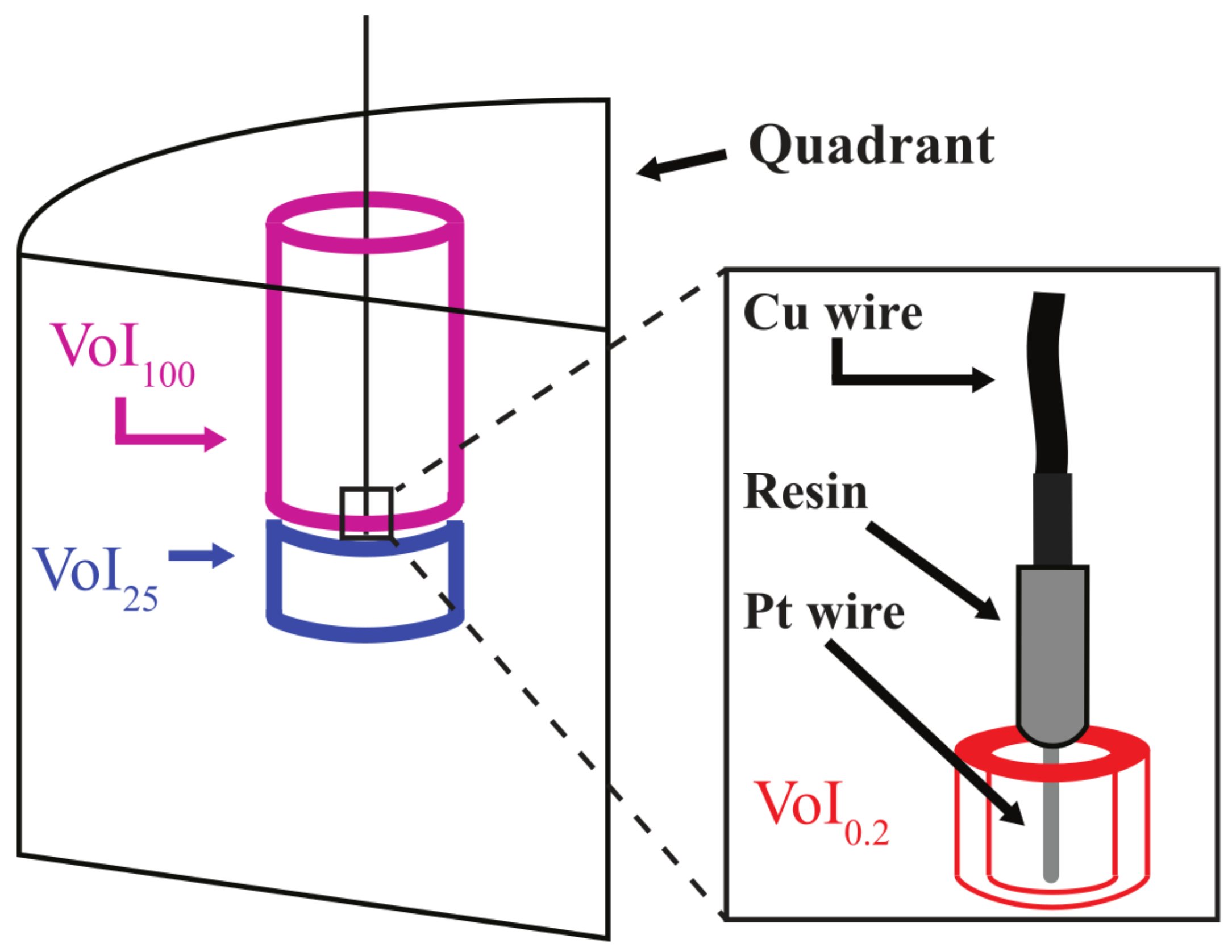
The available energy sensed by the Pt-electrode tip represents the state of the soil solution in the pore system connecting the soil surface and the electrode tip. The resulting Volume of Interest (VoI100) was of a cylindrical shape centered around the electrode with a height of approximately 8 cm (minor variations between individual cylinders), a diameter of 4 cm, and an average volume of 100 mL.
(b)
The potential sensed represents a more constrained, but still sizable, region right below the electrode tip. This VoI had a diameter of 4 cm and extended 2 cm down from the bottom of the probe tip, resulting in a volume of approximately 25 mL (VoI25).
(c)
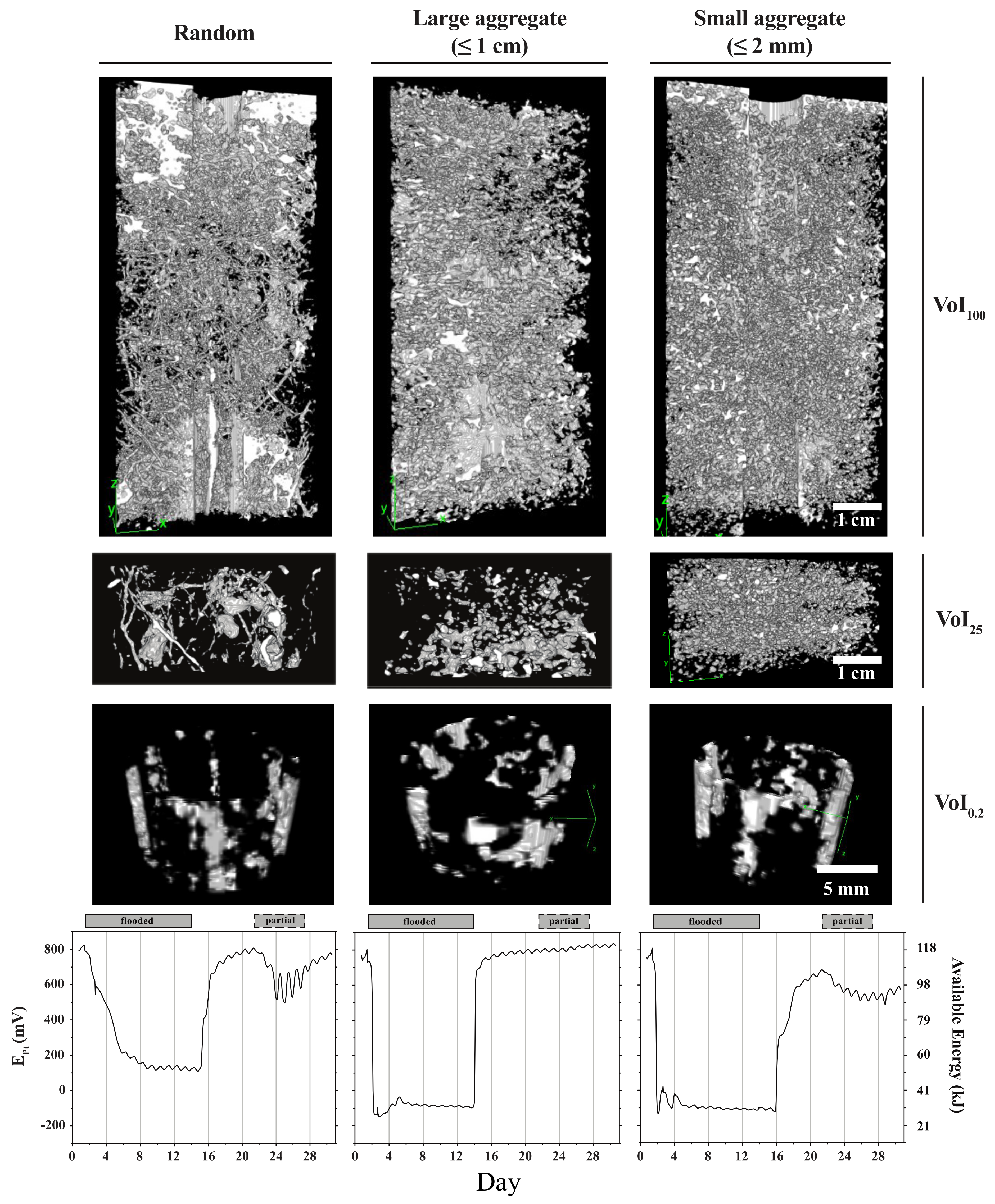
Testing the suggestion of Fiedler [33] that Pt-electrodes are only sensitive to the conditions in a space of few cubic mm immediately surrounding and connected to the platinum tip, we finally selected a volume of interest surrounding the platinum wire in the fashion of a cylindrical sleeve with a height of 7 mm, an inner diameter of 5 mm, and a wall thickness of 0.84 mm, yielding a volume of 190 mm3 or approximately 0.2 mL (VoI0.2). The dimensions of the inner core were chosen to avoid image artifacts created by the metal of the probe tip. Figure 4 demonstrates how the respective images varied as a function of pore network structure. Representative curves are added to reiterate significant differences in available energy dynamics. For each sub-sampled VoI, the contrast was set using Fiji’s auto brightness/contrast setting. The binary threshold was then set manually by comparing pore edges in four different images to the same pore edges in the corresponding images from the 8-bit image stack prior to thresholding [45]. A 3D median filter of the dimensions, 5 × 5 × 5 pixels, was then applied to each binary stack, which reduced noise, but preserved pore edges [46].

2.2.3. Image Analyses

To quantify the pore space architecture, each thresholded sub-sample was analyzed with the help of two sets of metrics (pore network metrics, PNM). One set of metrics (skeleton-based metrics, # 1–9 in Table 1; Figure 3) was used to describe the interconnectedness and complexity of the pore network in the VoI, while a second set (void-based metrics, # 10–18 in Table 2; Figure 3) was used to characterize the three-dimensional reaction space that the pores occupied. The skeleton network of the pore space is generated by eroding the voxels defined as pores in each image down to their single voxel width medial axes. A skeleton network is defined as all interconnected medial axes, and a single image stack can be comprised of multiple skeleton networks. The medial axes for each image stack were generated using the Skeletonize3D plugin [47] and the shortest branches in circular skeletons were pruned. Analysis of the medial axes of each sample using the AnalyzeSkeleton plugin [48] generated the skeleton-based pore network metrics (Table 1; Figure 5). The void-based metrics (Table 2; Figure 5) were calculated using the Particle Analyzer function of the BoneJ plugin as well as the Bone Volume to Total Volume plugin to calculate the image based percent porosity [49]. All pore network metrics generated by the above plugins as well as the metrics calculated using the output from the above plugins are visualized in Figure 5.

2.3. Statistics

Statistics were performed using either OriginPro (Version X, OriginLab, Northampton, MA, USA) or RStudio for Mac version 1.0.136 [52]. All PNMs were normalized to a unit per mm3 basis. Linear regression was carried out between the mean value for each pore network metric (PNM; explanatory) and the value for each available energy metric (AE-metric; response). A relationship between a PNM and an AE-metric was deemed significant at the p < 0.05 level when the r2 value from a given regression was greater than or equal to 0.44 (n = 9 VoIs per PNA, each representing one quadrant as illustrated in Figure S3, d.f. = 8, f-value = 5.59). A two-tailed t-test was used to determine if there were significant differences between available energy metrics within a given pore network architecture (Table S2). Tukey’s honest significant difference test in RStudio was used to determine if there were significant differences between the mean values (n = 9) from each PNA for (i) the pore network metrics for each volume of interest (Tables S3–S5) and (ii) the available energy metrics (Table S6).

3. Results and Discussion

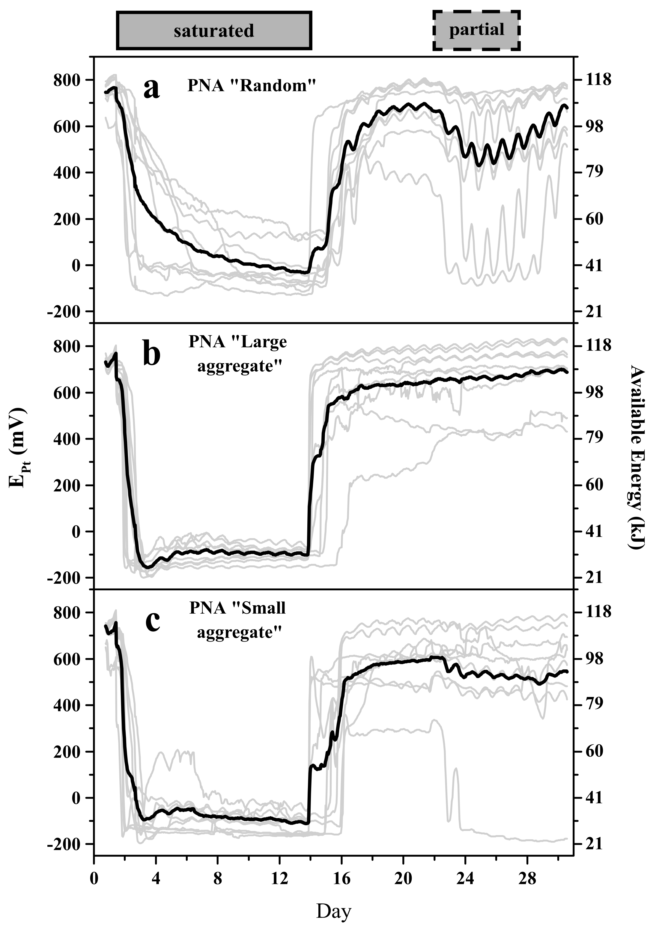
3.1. Pt-Electrodes Provide Robust and Reliable Information about Available Energy

There have been concerns about the ability of platinum electrodes to return meaningful data [53,54]. These concerns are based on limitations of the Pt-electrode system and on the multispecies, non-equilibrium nature of the soil solution [55]. Thus, when early researchers [56] noted deviations of more than 300 mV among replicate Pt-electrodes installed in the same soil horizon, they attributed such variability to the technical deficiencies of the Pt-electrode. An alternative explanation for variation among replicate electrodes installed in the same soil horizon would be that they are probing biogeochemically distinct microenvironments [32,33].
In our setting, 27 soil-electrode systems were subjected to the same changes in moisture content and all electrodes showed the same general response to changes in moisture content, with modifications specific to the respective pore network architectures (Figure 1). For instance, in the “Large Aggregate” pore network architecture (Figure 1, panel b), all nine electrodes registered the same rapid initial decrease in available energy (=AE-metric a, Figure 2). This response is nearly identical in the “Small Aggregate” pore network architecture (Figure 1, panel c) while the nine electrodes installed in the “Random” pore network architecture with its native soil structure showed a much wider range of trajectories and associated slopes of the AE parameter “a” (Figure 1, panel a). We take these observations as supporting the view of Cogger, Kennedy and Carlson [32] and Fiedler [33] that variations among the potentials registered by multiple, well calibrated Pt-electrodes installed in the same soil horizon indicate corresponding variations in the biogeochemical states of the microenvironments probed by the respective electrodes. Figure 1 further suggests the existence of a complex link between pore network architecture and moisture state.
During the first inundation phase and while completely saturated, the potential registered by the n = 9 electrodes in the “Large Aggregate” and “Small Aggregate” PNAs behave very similarly in terms of timing and absolute value of the mean minimum electromotive potentials achieved (about −150 mV). (Figure 1, panels b and c). However, the mean minimum electromotive potential in the “Random” PNA continued to decrease over the entire period of complete inundation, only reaching a minimum value near 0 mV (Figure 1, panel a). Following the second, partial inundation (days 22–27.5, Figure 1), however, biogeochemical conditions in the PNA “Random” (Figure 1, panel a) begin to diverge widely while they stay relatively similar (with outliers) in the PNA’s “Large Aggregate” and “Small Aggregate” (Figure 1, Panels b and c). These findings allow us to accept hypothesis 1 (AE-metrics are ± constant within the same pore network) with the qualification that over time, the “Random” PNA (Figure 1, panel a; Table S2) offers greater opportunities for diverse biogeochemical conditions to evolve independently in individual microenvironments.

3.2. The Pore Network Metric—Pore Network Architecture Relationship Depends on the Observed Soil Volume

The values of the pore network metrics (PNMs) chosen to quantify variations in pore network architecture varied as a function of both network architecture and VoI. This can be illustrated using PNM # 11: “Average Void Surface Area” as an example (for definition and illustration of PNM 11 see Table 2 and Figure 5). Depending on the VoI considered, PNM values can be near identical across pore network architectures (VoI0.2, Table S3), or significantly different (VoI25, Table S4). An analysis including all 18 PNMs (Tables S3–S5) reveals that the occurrence of significant differences between PNAs is greatest in the 25 mL VoI (30 significant differences, Table S4), followed by the 100 mL VoI (17 significant differences, Table S3) while PNMs in the 0.2 mL VoIs were largely constant, with only two significant differences observed across PNAs. This trend is consistent with the fact that the selection of a small VoI will necessarily limit the abundance of larger sized, more complex pores within the observed VoI.
VoIs showed largely constant behavior across PNAs with only two significant differences observed. This trend is consistent with the fact that the selection of a small VoI will necessarily limit the abundance of larger sized, or complex pores within the observed VoI. The XCT analysis most closely scaled to the dimensions of the soil pore network investigated in our study was carried out by Köhne, et al. [57], who sampled two soils of contrasting texture using three different sample container sizes. Though assessing the role of the pore network in regulating contaminant movement in soils as a function of the scale of observation, their results suggest an intimate relationship between the pore network structure and function for physical transport processes. To a similar end, where possible, we compared the resulting pore network information in an effort to capture both the larger interaggregate pores and the smaller intra-aggregate pores from a single sample.

3.3. Pore Network Architecture Modifies Available Energy

The pore network has been thought to play a role in redox dynamics in soils for nearly 70 years [58,59,60]. Assessments of the extent to which the redox status of the soil and the pore network are related usually end at differentiating between macro and micro pores (e.g., [61]) or changes in porosity overall (e.g., [61]). Most major models of aerobic or anaerobic microsite formation depend on estimating water-filled porosity or air-filled porosity to calculate diffusion coefficients (of gases or dissolved organic carbon) and generally ignore pore network structure [7]. X-ray computed tomography provides a method to more directly measure the structure of the pore network and its impacts on soil processes. However, most applications focus on quantification of water fluxes [62], saturated hydraulic conductivity [63,64], air fluxes [65,66,67], or pore space genesis as a function of microbial activity [68], and not directly on the formation (or location) of microbial ‘hotspots’ (i.e., anaerobic soil volumes) [9]. Part of this may be due to the complex relationship between the pore network and microbial activity; even studies specifically designed to generate contrasting results have not necessarily produced conclusive outcomes [15]. To the best of our knowledge, very little attention has been paid to purposefully manipulating the pore network and quantifying the resulting changes in electromotive potential dynamics (e.g., [61]).
To test the null-hypothesis, “the dynamics of available energy are independent of pore network architecture”, we evaluated the extent to which available energy (AE) metrics (Figure 2) differed between individual PNAs. To do so, the Tukey’s honest significant differences test was used to compare the means of all 10 AE-metrics developed to describe the dynamics of available energy during the duration of the experiment (Table S6). The greatest number of significant differences, six in total, was registered when comparing the PNA “Random” with the PNA “Large Aggregate”. The significant differences occurred between AE-metrics a, b, c, d, f, and i (Table S6). Only one AE-metric had a borderline significant p-value (p = 0.073) in the Random—Large Aggregate comparison (AE-metric j). There were two significant differences and one borderline significant difference in AE-metrics when the Random and Small Aggregate PNAs were compared (significant: c and d; borderline b, p-value = 0.053). The AE-metrics for the Large and Small Aggregate PNAs were very similar, with only one borderline significant difference identified between the AE-metrics (AE-metric d, p-value = 0.066). We refute the null hypothesis that available energy is independent of pore network architecture based on the clear differences noted in the comparison between the random (or native soil structure) and artificially created structures. To our surprise, there were no significant differences in available energy between the two artificially created PNAs, indicating that aggregate size is not likely to be the sole controlling factor in the dynamics of available energy.

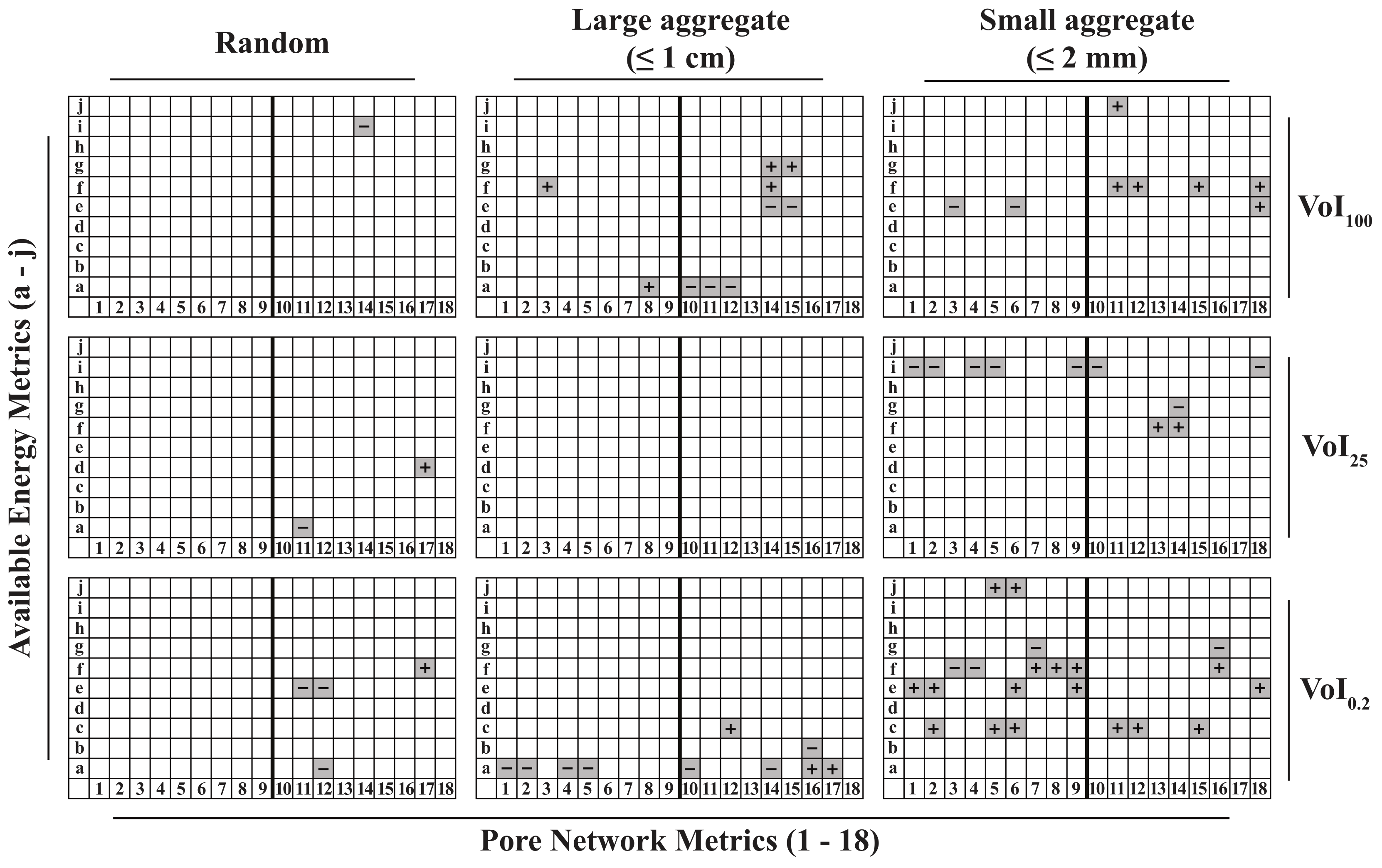
3.4. Pore Network Metrics Have Differential Power to Explain Available Energy Metrics

The pore network architecture is traditionally parameterized by generating moisture release functions, a method that has been extensively used in the soil physics community. However, these functions are typically obtained using soil samples in the 3 to 10 cm size range and the resulting information provided on pore characteristics is an average across the entire sample [69]. For example, basic physical soil properties were not significant predictors of saturated hydraulic conductivity when compared to XCT derived macropore characteristics [63].
The use of 3D XCT to quantify the structure of the soil pore network has become almost ubiquitous in recent years. Because of this, the associated parameters have become equally broad ranging. These parameters can be broken down into two major categories: (1) Parameters that describe the reaction space (i.e., the 3D pore space itself) and (2) parameters that describe the complexity or connectivity of the pore network (i.e., the number of pore connections per unit volume). Variables that belong to the first category are: Visible porosity [15,64,70,71,72,73], pore size distribution [50,70,73,74], pore surface area [75,76,77], pore thickness (i.e., diameter) [71,77,78], and total visible pore volume [42,50,79]. Variables that fall in the second category rely largely on what is referred to as the skeleton, or single voxel width medial axes, of the pore network [47,80]. Examples here include: Tortuosity, calculated as total pore length/Euclidean distance [42,46,50,81] or using the Euler number [57,74,82]; pore connectivity, calculated using (i) Euler number [75,83] or (ii) node density [50,67]; macropore length [42,50]; and percolating pores [78].
Nine correlation matrices (three pore network architectures versus three volumes of interest, Figure 6) were constructed to explore the existence of linear correlations between available energy metrics (AE, dependent variable) and pore network metrics (PNMs, predictor variable). In these matrices (Figure 6), the ability of each pore network metric (1…18) to predict any of the available energy metrics (a…j) is represented by either a plus (positive correlation) or a minus symbol (negative correlation). The existence of a significant correlation was assumed if the coefficient of determination (r2) for the relationship between the respective PNM and a given AE-metric (n = 9 for each combination of PNA and VoI) was ≥0.44 (f-value = 5.59, d.f. = 8).
Examination of the entire cohort of nine correlation matrices allows the assessment of the ability of somewhat arbitrarily chosen metrics to quantify the relationship between soil structure and available energy dynamics. Figure 7a compares the ‘efficiency’ of individual AE-metrics as descriptor variables and shows that variables f, a, and e were much more often correlated with a pore network metric than any of the other AE-metrics. Figure 7a also illustrates the abundance of positive versus negative correlations. For instance, the rate of EPt increase (i.e., available energy increase) after the first drainage (AE-metric “f”) was mainly positively correlated with pore network metrics (PNMs), while the subsequent decline in EPt (i.e., available energy decrease) following partial inundation (AE-metric “i”) was always negatively correlated with PNMs.
A similar analysis can be conducted for the PNMs. Here, we find that void-base metrics (Figure 7c) tend to appear more frequently in significant correlations with AE-metrics than skeleton-based metrics (Figure 7b), with particularly high scores noted for PNMs 14 (seven instances), 12, and 11 (six and five instances, respectively). Overall, void-based pore network metrics correlate on a total of 38 occasions compared to 28 total correlations observed for skeleton-based metrics (Figure 7b,c). Considering subtotals for the three different PNAs, we find a trend of an increasing number of correlations going from PNA “Random” with seven total correlations, 20 correlations for the PNA “Large Aggregate”, to 39 correlations in the PNA “Small Aggregate” (Figure 8a). We found that the void-based pore network metrics tended to have statistically stronger relationships with AE-metrics, evidenced by way of a greater total number of significant correlations compared to the skeleton-based metrics.
As the shape, size, or layout of the pore network changes, so must the relationship with available energy, and subsequently the existence or lack of statistically significant correlations. We decided to investigate four categories of AE-metrics, each representing different functionalities of the pore network: (i) Decreasing EPt (negative slopes)—represents water movement into the pore network, an increasing restriction on the resupply of atmospheric oxygen, and a facilitation of nutrient diffusion and advection; (ii) extreme EPt values (maximums or minimums)—are seen as capacitive indicators, potentially useful to parameterize boundary conditions for the system studied. A soil not returning to fully aerobic state (high EPt) after rewetting may have a pore system with poor connectivity, while a soil unable to achieve low available energy (low EPt) may lack electron donors, such as reduced organic matter; (iii) timing of minimum or maximum potentials—along with the pore characteristics necessary for point (ii) above, the timing of the extreme values depends on the rate at which water can flow in or out as well as the rate at which nutrients or gases can move through the pore network; and (iv) increasing EPt—requires that water flow out of the pore network in an unrestricted fashion, but, more importantly, the uninhibited reentry of oxygen into the pore network.
Though the void-based PNMs incurred a higher total number of correlations compared to the skeleton-based PNMs, the correlation of a void-based or skeleton-based PNM with an AE-metric was always a function of VoI and PNA. In the “Small Aggregate” PNA, as the VoI decreased, the number of significant correlations with skeleton-based metrics increased while they decreased in the void-based metrics. This suggests that the reactions occurring in immediate proximity to the Pt-electrode tip are more dependent on the connectivity of the pore network and not so much on the magnitude of reaction space provided by the pores. The formation of anaerobic conditions (or ‘hotspots’) at scales beyond the immediate vicinity of the Pt-electrode tip is likely more dependent on advective movement of gases (e.g., oxygen) and solutes (e.g., nutrients and DOC) through macropores [9] as opposed to diffusion-based transport, which has been thought to be the dominant mechanism in micropores [7,15]. We summarize that our exploratory analysis of the relationship between pore network parameters and parameters across different pore network architectures and volumes of interest suggests the existence of a set of parameters with the potential to be particularly useful for the investigation of structure—functionality relationships in soils.

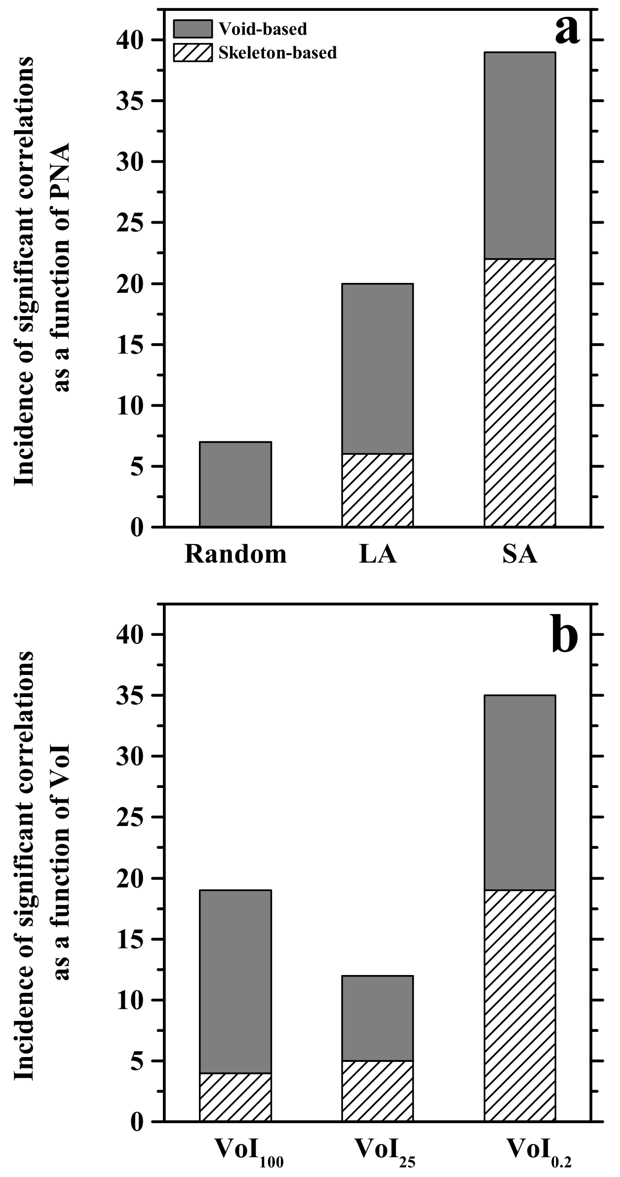
3.5. The Explanatory Power of PNMs Depends on Pore Network Architecture

This picture becomes more differentiated when correlations between PNMs and AE-metrics are examined separately for each individual pore network architecture (PNA) and volume of interest (Figure 6 and Figure 8a,b). Within the native pore structure (aka PNA “Random”) none of the skeleton-based pore network metrics correlate with any of the AE-metrics (Figure 6 and Figure 8a). The void-based metrics show one, two, and four correlations going from VoI100, to VoI25, to VoI0.2, respectively (Figure 6). Of the three PNAs and across all VoIs, the PNA “Random” had the fewest total number of correlations (Figure 8a).
The total number of correlations increased to 20 for the PNA “Large Aggregate”, with six contributed by skeleton-based metrics and 14 involving void-based metrics (Figure 8a). In this PNA there was no trend with VoI: 10 correlations were found for the large VoI100, zero for the intermediate VoI25, and 10 for the small VoI0.2 (Figure 6 and Figure 8b). The correlations observed for the VoI100 were generally not the same as the ones observed for the VoI0.2. There was one combination of metrics (AE-metric “a” as a function of PNM “10”) that showed a significant negative correlation in both the VoI100 and VoI0.2 (Figure 6).
In the “Small Aggregate” pore network architecture (PNA), where the soil had been sieved to ≤ 2 mm, 39 correlations between AE-metrics and PNMs were found. Within this PNA, correlations involving skeleton-based metrics increased from two, to five, to 15 with decreasing VoI size (Figure 6), while correlations involving void-based metrics remained nearly constant as the VoI changed. Considering both skeleton and void-based metrics together, we observed a progression from eight, to 10, to 21 correlations going down in VoI size from VoI100, to VoI25, to VoI0.2, respectively (Figure 6). Out of 39 correlations observed for PNA “Small Aggregate”, only two combinations occurred in more than one of the VoIs, and both involved AE-metric “e”: This metric correlated negatively with PNM 6 in VoI100 and positively in VoI0.2. It also correlated positively with PNM 18 in both, VoI100 and VoI0.2. We observed only one incidence of correlation occurring between the same parameter pair across pore network architectures: AE “c” was negatively correlated with PNM “12” in PNA “Large Aggregate” and in the PNA “Small Aggregate” (Figure 6).
The observed effects of manipulating the pore network varied as a function of VoI. We assumed that the pore network would become more homogeneous in terms of both void and skeleton-based metrics as aggregate-size decreased (reflected as smaller coefficients of variation). While this trend was somewhat evident in VoI0.2 (coefficient of variation is similar across all PNMs, Table S5), most of the pore network metrics from the “Large Aggregate” PNA tended to be more variable than those from the “Random” or “Small Aggregate” pore network architectures in the two larger VoIs (coefficients of variation in Tables S3 and S4). What arose by sieving the soil to ≤1 cm for the “Large Aggregate” PNA was to effectively increase the pore network heterogeneity per unit volume.
An outcome of manipulating the pore network architecture (PNA) and varying the scale of observation was contrasting results in terms of the types of relationships between AE-metrics and PNMs. An example of VoI changing the relationship was in the “Small Aggregate” PNA. AE-metric “e” (Figure 2) correlated negatively with PNM 6 (number of junctions with four branches; Figure 4 and Table 1) in VoI100 and positively in VoI0.2 (Figure 6). In VoI100, as the number of junctions with four branches increased, the lag time from the first drain to an EPt increase of at least 50 mV became shorter. Because the 100 mL VoI was connected to the surface, as the number of pore connections from the electrode tip to the soil surface increased, oxygen was able to reach the electrode more quickly [84,85,86], thus decreasing the time required for the electromotive potential to change. In VoI0.2, the opposite occurred, as the number of quadruple points increased, the lag time also increased. A large number of connections implies that there are many branches/pores in the immediate vicinity of the Pt-electrode. As the number of branches/pores increases the pore volume able to be occupied with water increases, it would then take longer for the pore network to drain and oxygen to reach the electrode tip [87].
An example of the type of change in relationship between AE-metrics as a function of PNA occurred in the “Random” and “Large Aggregate” PNAs and pore network metric “12” (Figure 5 and Table 2; average enclosed void volume). In the same VoI (VoI0.2), PNM “12” correlated negatively with AE-metric “a” (Figure 2; rate of available energy decrease over the first 72 h after inundation) in the “Random” PNA, while the same PNM correlated positively with AE-metric “c” (Figure 2; maximum available energy during pore network inundation) in the “Large Aggregate” PNA. In the “Random” PNA, as the enclosed void volume increased, the rate at which available energy increased over the first 72 h after flooding became increasingly negative (the rate of change became larger). In the “Large Aggregate” PNA, as the enclosed void volume increased, the maximum available energy increased (EPt became less negative). These results suggest that the relationship between pore network metrics and available energy dynamics is a function of aggregate size, and by extension, the pore network architecture of the system as a whole. Therefore, the establishment and scaling of such a relationship must take in to account the pore network architecture across a sufficiently sized representative elementary volume to capture the majority of aggregate sizes.

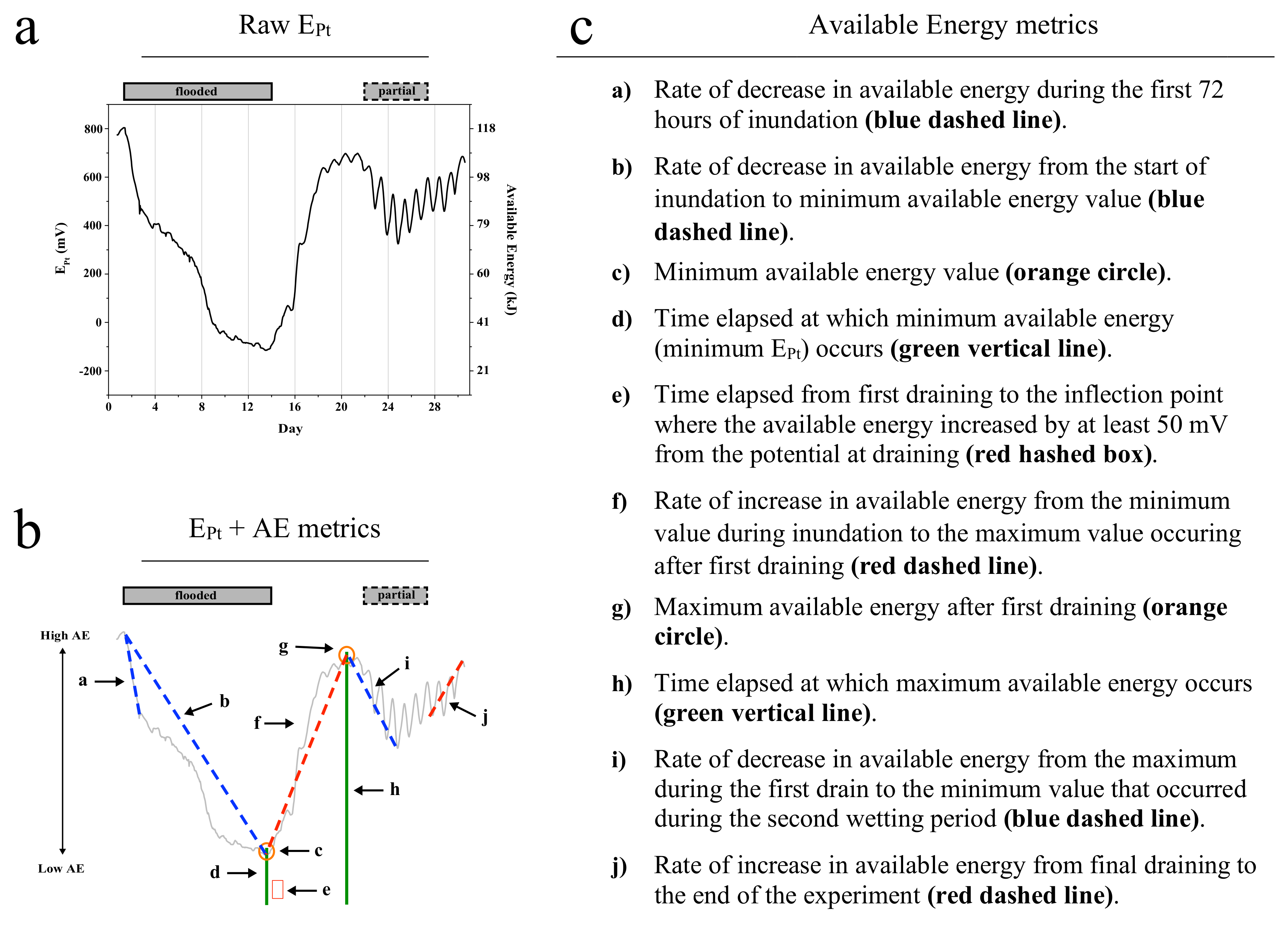
3.6. Utility of Available Energy and Pore Network Metrics

Not all available energy or pore network metrics were equally useful in describing the available energy dynamics over the duration of our experiment. Of the 66 total correlations between AE-metrics and PNMs, Figure 7a shows that three out of the 10 AE-metrics accounted for over half of those correlations (41 in total). Those AE-metrics (defined in Figure 2) were: “a” (rate of decrease in EPt during the first 72 h after inundation), “e” (time elapsed from first draining to the inflection point where the available energy increased by at least 50 mV from the potential at draining), and “f” (rate of increase in EPt from the minimum value during inundation to the maximum value occurring after first draining).
Similarly, there were certain pore network metrics (described in Table 1 and Table 2, and Figure 5) that correlated more often with AE-metrics than others. The top three skeleton-based metrics (Figure 7b) were all concerning the number of pore junctions: “2” (total number of junctions), “5” (the number of junctions with exactly three branches), and “6” (the number of junctions with exactly four branches). The top three void-based metrics (Figure 7c) were: “11” (void surface area), “12” (enclosed void volume), and “14” (the standard deviation of the mean pore diameter). These results indicate that certain aspects of AE dynamics are more closely regulated by the pore network compared to others. Similarly, the pore network metrics that were most often correlated with changes in AE-metrics were those that have been directly tied to gas [67,81] and water movement [e.g. 61] through the pore network.

3.7. The Explanatory Power of PNMs Is Greatest for a Small Soil Volume Immediately Surrounding the Electrode Tip

Size and placement of the soil volume observed were found to have a profound influence on the ability of PNMs to statistically explain variations in available energy metrics (Figure 8b). In VoI100, pore network metrics were mostly correlated with AE parameters “f” (six incidences, all positive) and “e” (five incidences, four negative, one positive). Out of 19 total correlations observed for this volume, only one occurred in the PNA “Random” (Figure 6). In VoI25, 7 PNMs correlated with AE-metric “i”, these correlations occurred in PNA “Small Aggregate” and all of them were negative. More than half (35 out of 66 total) of all observed correlations occurred in VoI0.2; with AE variable “a” showing nine correlations while variables “c”, “e”, and “f” had seven correlations each. Correlations with AE variable “a” occurred overwhelmingly in PNA “Large Aggregate”, while correlations with variables “c”, “e”, and “f” mostly occurred in the PNA “Small Aggregate”. This finding can be seen as supportive of the hypothesis that the Pt-electrode is most sensitive to the electrochemical conditions immediately surrounding the platinum wire tip, as proposed by Fiedler [33].
AE-metric “i” is the rate at which available energy decreases during the second, partial fill, with water. Water movement to the electrode tip during this portion of the experiment is dependent entirely on capillary rise. It stands to reason then that the portion of the pore network that is most related to these dynamics would be the portion of the pore network immediately below the Pt-tip. This assessment partially breaks down on one other occasion in the “Random” PNA where AE-metric “i” significantly correlates (again in a negative fashion) with PNM 14 (SD of mean pore diameter), but this time in VoI100. Though the 100 mL VoI does not quantify the pores directly responsible for capillary movement of water, it does capture the pores surrounding the electrode tip. These pores will still be responsible for movement of water from the ‘water table’ (water level during the second, partial inundation) to the electrode tip. Though the XCT resolution in this study did not allow for pores < 220 µm to be resolved, we know that such pores exist in abundance. However, knowing that there are smaller pores in the soil, which will inevitably lead to capillary rise, we feel justified to tentatively attribute the correlation between these ‘coarse’ pores and AE-metric “i” to capillary rise.
Significant differences in AE-metrics between pore network architectures do not always mean that there will be significant correlations between those AE-metrics and pore network metrics. For example, AE-metrics “c” and “d” (the time elapsed at which the minimum available energy occurs) were significantly different between the “Random” and “Large Aggregate” (p < 0.001), and “Random” and “Small Aggregate” (p < 0.01) pore network architectures Table S6). However, AE-metric “d” only had one total significant correlation across all VoIs and pore network architectures (Random VoI25, PNM = 16) whereas AE-metric “c” had a total of seven: “Large Aggregate” VoI0.2, PNM = 12 (positive) and “Small Aggregate” VoI0.2, PNMs = 2, 5, 6, 11, 12, 15 (all positive) (Figure 6).
AE-metric “b” only had one significant correlation in all VoIs and pore network architectures (VoI0.2, PNA = “Large Aggregate”, PNM = 16) (Figure 6). The lack of correlations could be explained by the fact that we completely flooded the pore networks, so the electromotive potential was left no choice, but to decrease, and the pore network had little to no opportunity to influence the decrease. If this were the explanation, then there should have been no significant difference in the rate of electromotive potential decline. However, AE-metric “b” was significantly different between the “Random” and “Large Aggregate” pore network architectures (p < 0.05) and nearly significant between the “Random” and “Small Aggregate” pore network architectures (p = 0.053; Table S6).
We registered the strongest statistical relationship between AE-metrics and the pore network when examining the pores immediately surrounding the Pt-electrode. One possible explanation for the increased number of significant correlations between AE-metrics and PNMs in the smallest VoI and PNA with the smallest pores is: As aggregate size decreased, large biopores, with smooth, potentially hydrophobic surfaces [88], were increasingly destroyed. This lead to redistributed (i.e., more easily accessible) electron sources [15] and the generation of rough pore surfaces [70,89,90]. Rough pore surfaces have been shown to collect small, yet significant, pools of water [91], provide more attachment points and habitable niches for microbes [62,92,93], along with increased diffusion of nutrients in the pore water [94]. This result is also consistent with the assessment made by Fiedler [33] that the Pt-electrode is most sensitive to the soil volumes and biogeochemical processes that are in immediate, direct contact.
We summarize that the mechanisms that regulate water, gas, and nutrient transport (which ultimately control available energy) are different across scales. At larger scales, water, gases, and nutrients are dominantly moved by advection, while at smaller scales, diffusive movement dominates. The PNMs that more tightly regulate diffusion (e.g., pore tortuosity or the number/class of pore connections) will correlate at the small VoI, while the PNMs that are more involved in advective movement (e.g., SD of mean pore diameter or void surface area) will correlate more often at larger VoIs, or in the pore network architectures with larger aggregates/pores.

4. Conclusions

To the best of our knowledge, there has not yet been a report of an attempt to investigate variations in electromotive potential or redox status of soil environments with the help of metrics from three-dimensional imaging methods, such as computed tomography. Similarly, we are not aware of investigations that would have manipulated soil structure with the intent to explore resulting effects on the dynamics of soil redox status. We demonstrate that the pore network and the dynamics of electromotive potentials in soils are indeed correlated, but these correlations depended on both (i) the type of pore network architecture and (ii) the soil volume chosen for imaging analysis. We recognize an overall trend of increasing predictability as both aggregate sizes and volumes of interest get smaller, but there were exceptions to the trend that prevent us from making generalizing statements at this time. However, our work showed: The fact that a given CT-derived pore network metric does not have much predictive power in a certain type of structural environment and at a certain scale of observation does not necessarily mean that this would be the same in a different environment and at another scale of observation. Our findings suggest that future investigations of physiological processes in porous soil and subsurface systems should involve preliminary activities to determine the scale of observation (volume of interest) and the associated kind of pore network metric best suited to generate the answer sought.

Supplementary Materials

The following are available online at https://www.mdpi.com/2571-8789/2/4/66/s1, Figure S1: Experimental set up of PVC rings, Figure S2: Visual timeline of water saturation conditions, Figure S3: Example images of sub-samples and sub-sampling process, Table S1: Woodburn series characteristics for Ap horizon, 0–20 cm, Table S2: Significant differences between electron activity metrics with in the pore network architectures, Table S3: Significant differences in pore network metrics across pore network architectures for VoI100, Table S4: Significant differences in pore network metrics across pore network architectures for VoI25, Table S5: Significant differences in pore network metrics across pore network architectures for VoI0.2. Table S6: Significant differences in available energy metrics across pore network architectures.

Author Contributions

Conceptualization: T.W. and M.K. (Markus Kleber); Methodology: T.W., M.K. (Markus Kleber), M.K. (Marco Keiluweit), P.S.N., T.V., and S.F.; Formal Analysis: T.W. and M.K. (Markus Kleber). Investigation: T.W., T.V., and M.K. (Markus Kleber). Resources: T.V. and M.K. (Markus Kleber); Writing-Original Draft Preparation: T.W. and M.K. (Markus Kleber); Writing-Review & Editing: M.K. (Marco Keiluweit), P.S.N., S.F., T.W., T.V., and M.K. (Markus Kleber); Visualization: A.L. and T.W.; Supervision: M.K. (Markus Kleber); Project Administration: M.K. (Markus Kleber) and S.F.; Funding Acquisition: S.F., M.K. (Markus Kleber) and P.S.N.

Funding

This work was supported by the US Department of Energy, Office of Biological and Environmental Research, Terrestrial Ecosystem Program (Award Number DE-FG02-13ER65542) and Subsurface Biogeochemistry Program (Award Number DE-SC0016544). Parts of this work were supported by the Environmental Molecular Sciences Laboratory (EMSL), a user facility at the Pacific Northwest National Laboratory at Richland, WA through user proposals 48704 (Kleber); 48750 (Kleber) and 48910 (Fendorf).

Conflicts of Interest

The authors declare no conflict of interest. The funders had no role in the design of the study; in the collection, analyses, or interpretation of data; in the writing of the manuscript, and in the decision to publish the results.

References

  1. Wania, R.; Ross, I.; Prentice, I.C. Integrating peatlands and permafrost into a dynamic global vegetation model: 2. Evaluation and sensitivity of vegetation and carbon cycle processes. Glob. Biogeochem. Cycles 2009, 23. [Google Scholar] [CrossRef] [Green Version]
  2. Fendorf, S.; Michael, H.A.; van Geen, A. Spatial and temporal variations of groundwater arsenic in South and Southeast Asia. Science 2010, 328, 1123–1127. [Google Scholar] [CrossRef] [PubMed]
  3. Borja, J.; Taleon, D.M.; Auresenia, J.; Gallardo, S. Polychlorinated biphenyls and their biodegradation. Process Biochem. 2005, 40, 1999–2013. [Google Scholar] [CrossRef]
  4. Abramowicz, D. Aerobic and Anaerobic Biodegredation of PCBs: A Review. Crit. Rev. Biotechnol. 1990, 10, 241–251. [Google Scholar] [CrossRef]
  5. Riley, W.J.; Maggi, F.; Kleber, M.; Torn, M.S.; Tang, J.Y.; Dwivedi, D.; Guerry, N. Long residence times of rapidly decomposable soil organic matter: Application of a multi-phase, multi-component, and vertically resolved model (BAMS1) to soil carbon dynamics. Geosci. Model Dev. 2014, 7, 1335–1355. [Google Scholar] [CrossRef]
  6. Cussler, E.L. Diffusion: Mass Transfer in Fluid Systems, 2nd ed.; Cambridge University Press: New York, NY, USA, 1997. [Google Scholar]
  7. Keiluweit, M.; Nico, P.S.; Kleber, M.; Fendorf, S. Are oxygen limitations under recognized regulators of organic carbon turnover in upland soils? Biogeochemistry 2016, 127, 157–171. [Google Scholar] [CrossRef]
  8. McClain, M.E.; Boyer, E.W.; Dent, C.L.; Gergel, S.E.; Grimm, N.B.; Groffman, P.M.; Hart, S.C.; Harvey, J.W.; Johnston, C.A.; Mayorga, E.; et al. Biogeochemical Hot Spots and Hot Moments at the Interface of Terrestrial and Aquatic Ecosystems. Ecosystems 2003, 6, 301–312. [Google Scholar] [CrossRef]
  9. Kuzyakov, Y.; Blagodatskaya, E. Microbial hotspots and hot moments in soil: Concept & review. Soil Biol. Biochem. 2015, 83, 184–199. [Google Scholar] [CrossRef]
  10. Riley, W.J.; Subin, Z.M.; Lawrence, D.M.; Swenson, S.C.; Torn, M.S.; Meng, L.; Mahowald, N.M.; Hess, P. Barriers to predicting changes in global terrestrial methane fluxes: Analyses using CLM4Me, a methane biogeochemistry model integrated in CESM. Biogeosciences 2011, 8, 1925–1953. [Google Scholar] [CrossRef]
  11. Kuka, K.; Franko, U.; Rühlmann, J. Modelling the impact of pore space distribution on carbon turnover. Ecol. Model. 2007, 208, 295–306. [Google Scholar] [CrossRef]
  12. Davidson, E.A.; Samanta, S.; Caramori, S.S.; Savage, K. The Dual Arrhenius and Michaelis-Menten kinetics model for decomposition of soil organic matter at hourly to seasonal time scales. Glob. Chang. Biol. 2012, 18, 371–384. [Google Scholar] [CrossRef]
  13. Koven, C.D.; Riley, W.J.; Subin, Z.M.; Tang, J.Y.; Torn, M.S.; Collins, W.D.; Bonan, G.B.; Lawrence, D.M.; Swenson, S.C. The effect of vertically-resolved soil biogeochemistry and alternate soil C and N models on C dynamics of CLM4. Biogeosci. Discuss. 2013, 10, 7201–7256. [Google Scholar] [CrossRef]
  14. Keiluweit, M.; Wanzek, T.; Kleber, M.; Nico, P.S.; Fendorf, S. Anaerobic Microsites have an Unaccounted Role in Soil Carbon Stabilization. Nat. Commun. 2017, 8, 1771. [Google Scholar] [CrossRef] [PubMed]
  15. Negassa, W.C.; Guber, A.K.; Kravchenko, A.N.; Marsh, T.L.; Hildebrandt, B.; Rivers, M.L. Properties of soil pore space regulate pathways of plant residue decomposition and community structure of associated bacteria. PLoS ONE 2015, 10, e0123999. [Google Scholar] [CrossRef]
  16. Kravchenko, A.N.; Negassa, W.C.; Guber, A.K.; Hildebrandt, B.; Marsh, T.L.; Rivers, M.L. Intra-aggregate Pore Structure Influences Phylogenetic Composition of Bacterial Community in Macroaggregates. Soil Sci. Soc. Am. J. 2014, 78, 1924. [Google Scholar] [CrossRef]
  17. Ruamps, L.S.; Nunan, N.; Chenu, C. Microbial biogeography at the soil pore scale. Soil Biol. Biochem. 2011, 43, 280–286. [Google Scholar] [CrossRef]
  18. Wieder, W.R.; Bonan, G.B.; Allison, S.D. Global soil carbon projections are improved by modelling microbial processes. Nat. Clim. Chang. 2013, 3, 909–912. [Google Scholar] [CrossRef]
  19. Wieder, W.R.; Allison, S.D.; Davidson, E.A.; Georgiou, K.; Hararuk, O.; He, Y.J.; Hopkins, F.; Luo, Y.Q.; Smith, M.J.; Sulman, B.; et al. Explicitly representing soil microbial processes in Earth system models. Glob. Biogeochem. Cycles 2015, 29, 1782–1800. [Google Scholar] [CrossRef] [Green Version]
  20. Ruamps, L.S.; Nunan, N.; Pouteau, V.; Leloup, J.; Raynaud, X.; Roy, V.; Chenu, C. Regulation of soil organic C mineralisation at the pore scale. FEMS Microbiol. Ecol. 2013, 86, 26–35. [Google Scholar] [CrossRef] [Green Version]
  21. Angle, J.C.; Morin, T.H.; Solden, L.M.; Narrowe, A.B.; Smith, G.J.; Borton, M.A.; Rey-Sanchez, C.; Daly, R.A.; Mirfenderesgi, G.; Hoyt, D.W.; et al. Methanogenesis in oxygenated soils is a substantial fraction of wetland methane emissions. Nat. Commun. 2017, 8, 1567. [Google Scholar] [CrossRef] [Green Version]
  22. Ebrahimi, A.; Or, D. Dynamics of soil biogeochemical gas emissions shaped by remolded aggregate sizes and carbon configurations under hydration cycles. Glob. Chang. Biol. 2018, 24, 378–392. [Google Scholar] [CrossRef] [PubMed]
  23. Baas Becking, L.G.; Kaplan, I.R.; Moore, D. Limits of the Natural Environment in terms of pH and Oxidation-Reduction potentials. J. Geol. 1960, 68, 243–288. [Google Scholar] [CrossRef]
  24. Wanzek, T.; Keiluweit, M.; Baham, J.; Dragila, M.I.; Fendorf, S.; Fiedler, S.; Nico, P.S.; Kleber, M. Quantifying biogeochemical heterogeneity in soil systems. Geoderma 2018, 324, 89–97. [Google Scholar] [CrossRef]
  25. Bohn, H.L. Redox Potentials. Soil Sci. 1971, 112, 39–45. [Google Scholar] [CrossRef]
  26. Trumbore, S.E. Potential responses of soil organic carbon to global environmental change. Proc. Natl. Acad. Sci. USA 1997, 94, 8284–8291. [Google Scholar] [CrossRef] [Green Version]
  27. Hockaday, W.C.; Masiello, C.A.; Randerson, J.T.; Smernik, R.J.; Baldock, J.A.; Chadwick, O.A.; Harden, J.W. Measurement of soil carbon oxidation state and oxidative ratio by13C nuclear magnetic resonance. J. Geophys. Res. Biogeosci. 2009, 114. [Google Scholar] [CrossRef] [Green Version]
  28. Dincer, I. The role of exergy in energy policy making. Energy Policy 2002, 137–149. [Google Scholar] [CrossRef]
  29. Luo, L.; Lin, H.; Halleck, P. Quantifying Soil Structure and Preferential Flow in Intact Soil Using X-ray Computed Tomography. Soil Sci. Soc. Am. J. 2008, 72, 1058. [Google Scholar] [CrossRef]
  30. Nimmo, J.R.; Perkins, K.S. Effect of soil disturbance on recharging fluxes: Case study on the Snake River Plain, Idaho National Laboratory, USA. Hydrogeol. J. 2008, 16, 829–844. [Google Scholar] [CrossRef]
  31. Rabot, E.; Wiesmeier, M.; Schlüter, S.; Vogel, H.J. Soil structure as an indicator of soil functions: A review. Geoderma 2018, 314, 122–137. [Google Scholar] [CrossRef]
  32. Cogger, C.G.; Kennedy, P.E.; Carlson, D. Seasonally Saturated Soils in the Puget Lowland II. Measuring and Interpreting Redox Potentials. Soil Sci. 1992, 154, 50–58. [Google Scholar] [CrossRef]
  33. Fiedler, S. In-situ longterm measurements of redox potential in hydromorphic soils, in Redox Fundamentals. In Redox Fundamentals, Processes and Measuring Techniques; Schüring, J., Schulz, H.D., Fischer, W.R., Böttcher, J., Duijnisveld, W.H.M., Eds.; Springer: New York, NY, USA, 1999; pp. 81–94. [Google Scholar]
  34. Fiedler, S.; Vepraskas, M.J.; Richardson, J.L. Soil Redox Potential: Importance, Field Measurements, and Observations. Adv. Agron. 2007, 94, 1–54. [Google Scholar] [CrossRef]
  35. Staff, S.S. Kellogg Soil Survey Laboratory Methods Manual; Soil Survey Investigations Report No. 42; Burt, R., Staff, S.S., Eds.; U.S. Department of Agriculture, Natural Resources Conservation Service: Washington, DC, USA, 2014.
  36. Jones, R.H. Oxidation-Reduction Potential Measurement. ISA J. 1966, 13, 40. [Google Scholar]
  37. Austin, W.E.; Huddleston, J.H. Viability of permanently installed platinum redox electrodes. Soil Sci. Soc. Am. J. 1999, 63, 1757–1762. [Google Scholar] [CrossRef]
  38. Nordstrom, D.K.; Wilde, F.D. Field Measurements: Section 6.5 Reduction Oxidation Potential (Electrode Method). In National Field Manual for the Collection of Water Quality Data, 1.2 ed.; U.S. Geological Survey Office: Reston, VA, USA, 2005; Chapter A6. [Google Scholar]
  39. Taina, I.A.; Heck, R.J.; Elliot, T.R. Application of X-ray computed tomography to soil science: A literature review. Can. J. Soil Sci. 2008, 88, 1–20. [Google Scholar] [CrossRef]
  40. Tippkötter, R.; Eickhorst, T.; Taubner, H.; Gredner, B.; Rademaker, G. Detection of soil water in macropores of undisturbed soil using microfocus X-ray tube computerized tomography (μCT). Soil Tillage Res. 2009, 105, 12–20. [Google Scholar] [CrossRef]
  41. Pierret, A.; Capowiez, Y.; Belzunces, L.; Moran, C.J. 3D reconstruction and quantification of macropores using X-ray computed tomography and image analysis. Geoderma 2002, 106, 247–271. [Google Scholar] [CrossRef]
  42. Perret, J.; Prasher, S.O.; Kantzas, A.; Langford, C. Three-Dimensional Quantification of Macropore Networks in Undisturbed Soil Cores. Soil Sci. Soc. Am. J. 1999, 63, 1530. [Google Scholar] [CrossRef]
  43. Wildenschild, D.; Hopmans, J.W.; Vaz, C.M.P.; Rivers, M.L.; Rikard, D.; Christensen, B.S.B. Using X-ray computed tomography in hydrology: Systems, resolutions, and limitations. J. Hydrol. 2002, 267, 285–297. [Google Scholar] [CrossRef]
  44. Schindelin, J.; Arganda-Carreras, I.; Frise, E.; Kaynig, V.; Longair, M.; Pietzsch, T.; Preibisch, S.; Rueden, C.; Saalfeld, S.; Schmid, B.; et al. Fiji: An open-source platform for biological-image analysis. Nat. Methods 2012, 9, 676–682. [Google Scholar] [CrossRef]
  45. Quin, P.R.; Cowie, A.L.; Flavel, R.J.; Keen, B.P.; Macdonald, L.M.; Morris, S.G.; Singh, B.P.; Young, I.M.; Van Zwieten, L. Oil mallee biochar improves soil structural properties—A study with x-ray micro-CT. Agric. Ecosyst. Environ. 2014, 191, 142–149. [Google Scholar] [CrossRef]
  46. Jassogne, L.; McNeill, A.; Chittleborough, D. 3D-visualization and analysis of macro- and meso-porosity of the upper horizons of a sodic, texture-contrast soil. Eur. J. Soil Sci. 2007, 58, 589–598. [Google Scholar] [CrossRef] [Green Version]
  47. Lee, T.C.; Kashyap, R.L.; Chu, C.N. Building Skeleton Models Via 3-D Medial Surface Axis Thinning Algorithms. Cvgip Graph. Models Image Process. 1994, 56, 462–478. [Google Scholar] [CrossRef]
  48. Arganda-Carreras, I.; Fernandez-Gonzalez, R.; Munoz-Barrutia, A.; Ortiz-De-Solorzano, C. 3D reconstruction of histological sections: Application to mammary gland tissue. Microsc. Res. Tech. 2010, 73, 1019–1029. [Google Scholar] [CrossRef] [PubMed]
  49. Doube, M.; Klosowski, M.M.; Arganda-Carreras, I.; Cordelieres, F.P.; Dougherty, R.P.; Jackson, J.S.; Schmid, B.; Hutchinson, J.R.; Shefelbine, S.J. BoneJ: Free and extensible bone image analysis in ImageJ. Bone 2010, 47, 1076–1079. [Google Scholar] [CrossRef] [PubMed] [Green Version]
  50. Luo, L.; Lin, H.; Li, S. Quantification of 3-D soil macropore networks in different soil types and land uses using computed tomography. J. Hydrol. 2010, 393, 53–64. [Google Scholar] [CrossRef]
  51. Lorensen, W.E.; Cline, H.E. Marching Cubes: A High Resolution 3D Surface Construction Algorithm. Comput. Graph. 1987, 21, 163–169. [Google Scholar]
  52. RStudio, T. RStudio: Integrated Development for R; RStudio, Inc.: Boston, MA, USA, 2015. [Google Scholar]
  53. Bartlett, R.J. Characterizing soil redox behavior. In Soil Physical Chemistry; Sparks, D.L., Ed.; CRC Press: Boca Raton, FL, USA, 1998; pp. 371–397. [Google Scholar]
  54. Bartlett, R.J.; James, B.R. System for Categorizing Soil Redox Status by Chemical Field Testing. Geoderma 1995, 68, 211–218. [Google Scholar] [CrossRef]
  55. James, B.R.; Brose, D.A. Oxidation Reduciont Phenomena. In Handbook of Soil Sciences: Properties and Processes, 2nd ed.; Huang, Y.L., Malcolm, E.S., Eds.; CRC Press: Boca Raton, FL, USA, 2011; pp. 1–24. [Google Scholar]
  56. McKeague, J.A. Relationship od water table and Eh to Properties of three clay soils in the Ottawa Valley. Can. J. Soil Sci. 1965, 45, 49–62. [Google Scholar] [CrossRef]
  57. Köhne, J.M.; Schlüter, S.; Vogel, H.-J. Predicting Solute Transport in Structured Soil Using Pore Network Models. Vadose Zone J. 2011, 10, 1082. [Google Scholar] [CrossRef]
  58. Quispel, A. Measurement of the oxidation reduction potentials of normal and inundated soils. Soil Sci. 1947, 101, 265–275. [Google Scholar] [CrossRef]
  59. Grable, A.R.; Siemer, E.G. Effects of bulk density, aggregate size, and soil water suction on oxygen diffusiion, redox potentials, and elongatoin of corn roots. Soil Sci. Soc. Am. J. 1968, 32, 180–186. [Google Scholar] [CrossRef]
  60. Vepraskas, M.J.; Wilding, L.P. Aquic Moisture Regimes in Soils with and without Low Chroma Colors. Soil Sci. Soc. Am. J. 1983, 47, 280–285. [Google Scholar] [CrossRef]
  61. Zimmermann, I.; Fleige, H.; Horn, R. Soil structure amelioration with quicklime and irrigation experiments in earth graves. J. Soils Sediments 2016, 16, 2514–2522. [Google Scholar] [CrossRef]
  62. Or, D.; Smets, B.F.; Wraith, J.M.; Dechesne, A.; Friedman, S.P. Physical constraints affecting bacterial habitats and activity in unsaturated porous media—A review. Adv. Water Resour. 2007, 30, 1505–1527. [Google Scholar] [CrossRef]
  63. Luo, L.; Lin, H.; Schmidt, J. Quantitative Relationships between Soil Macropore Characteristics and Preferential Flow and Transport. Soil Sci. Soc. Am. J. 2010, 74, 1929. [Google Scholar] [CrossRef]
  64. Paradelo, M.; Katuwal, S.; Moldrup, P.; Norgaard, T.; Herath, L.; de Jonge, L.W. X-ray CT-Derived Soil Characteristics Explain Varying Air, Water, and Solute Transport Properties across a Loamy Field. Vadose Zone J. 2016, 15. [Google Scholar] [CrossRef]
  65. Rappoldt, C.; Crawford, J.W. The distribution of anoxic volume in a fractal model of soil. Geoderma 1999, 88, 329–347. [Google Scholar] [CrossRef]
  66. Naveed, M.; Moldrup, P.; Arthur, E.; Wildenschild, D.; Eden, M.; Lamandé, M.; Vogel, H.-J.; de Jonge, L.W. Revealing Soil Structure and Functional Macroporosity along a Clay Gradient Using X-ray Computed Tomography. Soil Sci. Soc. Am. J. 2013, 77, 403. [Google Scholar] [CrossRef]
  67. Katuwal, S.; Norgaard, T.; Moldrup, P.; Lamandé, M.; Wildenschild, D.; de Jonge, L.W. Linking air and water transport in intact soils to macropore characteristics inferred from X-ray computed tomography. Geoderma 2015, 237–238, 9–20. [Google Scholar] [CrossRef]
  68. Helliwell, J.R.; Miller, A.J.; Whalley, W.R.; Mooney, S.J.; Sturrock, C.J. Quantifying the impact of microbes on soil structural development and behaviour in wet soils. Soil Biol. Biochem. 2014, 74, 138–147. [Google Scholar] [CrossRef] [Green Version]
  69. Kravchenko, A.N.; Guber, A.K. Soil pores and their contributions to soil carbon processes. Geoderma 2017, 287, 31–39. [Google Scholar] [CrossRef]
  70. Kravchenko, A.N.; Negassa, W.C.; Guber, A.K.; Rivers, M.L. Protection of soil carbon within macro-aggregates depends on intra-aggregate pore characteristics. Sci. Rep. 2015, 5, 16261. [Google Scholar] [CrossRef] [PubMed] [Green Version]
  71. Larsbo, M.; Koestel, J.; Kätterer, T.; Jarvis, N. Preferential Transport in Macropores is Reduced by Soil Organic Carbon. Vadose Zone J. 2016, 15. [Google Scholar] [CrossRef] [Green Version]
  72. Rabbi, S.M.; Daniel, H.; Lockwood, P.V.; Macdonald, C.; Pereg, L.; Tighe, M.; Wilson, B.R.; Young, I.M. Physical soil architectural traits are functionally linked to carbon decomposition and bacterial diversity. Sci. Rep. 2016, 6, 33012. [Google Scholar] [CrossRef] [Green Version]
  73. Toosi, E.R.; Kravchenko, A.N.; Mao, J.; Quigley, M.Y.; Rivers, M.L. Effects of management and pore characteristics on organic matter composition of macroaggregates: Evidence from characterization of organic matter and imaging. Eur. J. Soil Sci. 2017, 68, 200–211. [Google Scholar] [CrossRef]
  74. Peth, S.; Horn, R.; Beckmann, F.; Donath, T.; Fischer, J.; Smucker, A.J.M. Three-Dimensional Quantification of Intra-Aggregate Pore-Space Features using Synchrotron-Radiation-Based Microtomography. Soil Sci. Soc. Am. J. 2008, 72, 897. [Google Scholar] [CrossRef]
  75. Sammartino, S.; Lissy, A.-S.; Bogner, C.; Van Den Bogaert, R.; Capowiez, Y.; Ruy, S.; Cornu, S. Identifying the Functional Macropore Network Related to Preferential Flow in Structured Soils. Vadose Zone J. 2015, 14. [Google Scholar] [CrossRef]
  76. Li, T.C.; Shao, M.A.; Jia, Y.H. Application of X-ray tomography to quantify macropore characteristics of loess soil under two perennial plants. Eur. J. Soil Sci. 2016, 67, 266–275. [Google Scholar] [CrossRef] [Green Version]
  77. Naveed, M.; Moldrup, P.; Schaap, M.G.; Tuller, M.; Kulkarni, R.; Vogel, H.-J.; Wollesen de Jonge, L. Prediction of biopore- and matrix-dominated flow from X-ray CT-derived macropore network characteristics. Hydrol. Earth Syst. Sci. 2016, 20, 4017–4030. [Google Scholar] [CrossRef]
  78. Jarvis, N.; Larsbo, M.; Koestel, J. Connectivity and percolation of structural pore networks in a cultivated silt loam soil quantified by X-ray tomography. Geoderma 2017, 287, 71–79. [Google Scholar] [CrossRef]
  79. Dong, H.; Blunt, M.J. Pore-network extraction from micro-computerized-tomography images. Phys. Rev. E Stat. Nonlinear Softw. Matter Phys. 2009, 80, 036307. [Google Scholar] [CrossRef] [PubMed]
  80. Arganda-Carreras, I. ImageJ Software Plug-in, Skeletonize, 3D 1.0.1, 2014.
  81. Katuwal, S.; Arthur, E.; Tuller, M.; Moldrup, P.; de Jonge, L.W. Quantification of Soil Pore Network Complexity with X-ray Computed Tomography and Gas Transport Measurements. Soil Sci. Soc. Am. J. 2015, 79, 1577. [Google Scholar] [CrossRef]
  82. Larsbo, M.; Koestel, J.; Jarvis, N. Relations between macropore network characteristics and the degree of preferential solute transport. Hydrol. Earth Syst. Sci. 2014, 18, 5255–5269. [Google Scholar] [CrossRef]
  83. Rabot, E.; Lacoste, M.; Hénault, C.; Cousin, I. Using X-ray Computed Tomography to Describe the Dynamics of Nitrous Oxide Emissions during Soil Drying. Vadose Zone J. 2015, 14. [Google Scholar] [CrossRef] [Green Version]
  84. Moldrup, P.; Olesen, T.; Komatsu, T.; Schønning, P.; Rolston, D.E. Tortuosity, Diffusivity, and Permeability in the Soil Liquid and Gaseous Phases. Soil Sci. Soc. Am. J. 2001, 65, 613–623. [Google Scholar] [CrossRef]
  85. Kawamoto, K.; Moldrup, P.; Schjønning, P.; Iversen, B.V.; Komatsu, T.; Rolston, D.E. Gas Transport Parameters in the Vadose Zone: Development and Tests of Power-Law Models for Air Permeability. Vadose Zone J. 2006, 5, 1205. [Google Scholar] [CrossRef]
  86. Tuli, A.; Hopmans, J.W. Effect of degree of fluid saturation on transport coefficients in disturbed soils. Eur. J. Soil Sci. 2004, 55, 147–164. [Google Scholar] [CrossRef]
  87. Tracy, S.R.; Daly, K.R.; Sturrock, C.J.; Crout, N.M.J.; Mooney, S.J.; Roose, T. Three-dimensional quantification of soil hydraulic properties using X-ray Computed Tomography and image-based modeling. Water Resour. Res. 2015, 51, 1006–1022. [Google Scholar] [CrossRef] [Green Version]
  88. Bachmann, J.; Guggenberger, G.; Baumgartl, T.; Ellerbrock, R.H.; Urbanek, E.; Goebel, M.-O.; Kaiser, K.; Horn, R.; Fischer, W.R. Physical carbon-sequestration mechanisms under special consideration of soil wettability. J. Plant Nutr. Soil Sci. 2008, 171, 14–26. [Google Scholar] [CrossRef]
  89. San José Martínez, F.; Muñoz Ortega, F.J.; Caniego Monreal, F.J.; Kravchenko, A.N.; Wang, W. Soil aggregate geometry: Measurements and morphology. Geoderma 2015, 237–238, 36–48. [Google Scholar] [CrossRef]
  90. Ananyeva, K.; Wang, W.; Smucker, A.J.M.; Rivers, M.L.; Kravchenko, A.N. Can intra-aggregate pore structures affect the aggregate’s effectiveness in protecting carbon? Soil Biol. Biochem. 2013, 57, 868–875. [Google Scholar] [CrossRef]
  91. Almquist, V.; Brueck, C.; Clarke, S.; Wanzek, T.; Dragila, M.I. Bioavailable water in coarse soils: A fractal approach. Geoderma 2018, 323, 146–155. [Google Scholar] [CrossRef]
  92. Massol-Deya, A.A.; Whallon, J.; Hickey, R.F.; Tiedje, J.M. Channel structures in aerobic biofilms of fixed-film reactors treating contaminated groundwater. Appl. Environ. Microbiol. 1995, 61, 769–777. [Google Scholar] [PubMed]
  93. Vandevivere, P.; Baveye, P.C. Saturated hydraulic conductivity reduction caused by aerobic bacteria in sand columns. Soil Sci. Soc. Am. J. 1992, 56, 1–12. [Google Scholar] [CrossRef]
  94. Or, D.; Tuller, M. Flow in unsaturated fractured porous media: Hydraulic conductivity of rough surfaces. Water Resour. Res. 2000, 36, 1165–1177. [Google Scholar] [CrossRef] [Green Version]
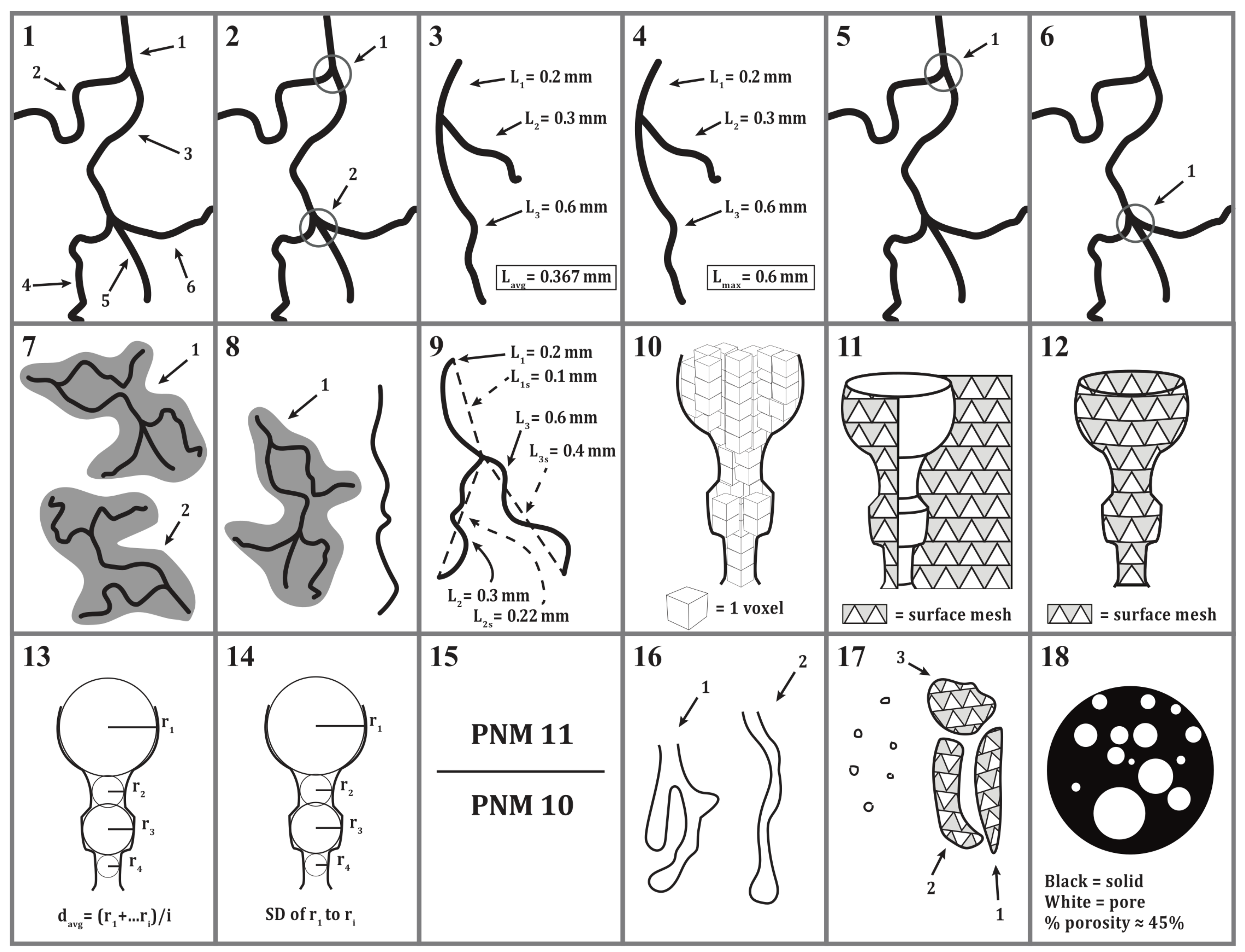
Figure 1. EPt curves for all three pore network architectures. Mean EPt curves (black) are shown for each pore network architecture: Random (a), Large Aggregate (b), and Small Aggregate (c). EPt data from each individual electrode per pore network architecture (n = 9 per pore network architecture) are also shown (gray). Available energy (kJ per electron transferred, right y-axis) was calculated assuming glucose (CH2O) as an electron donor and assuming standard temperature/pressure and soil pH. This is not a rigorously accurate determination of energy levels, but is meant to provide an energetic dimension to the EPt data. Timing and duration of complete saturation with water is represented by solid gray box “saturated” (day 1.5 to 14) and partial saturation is represented by dashed gray box “partial” (day 22 to 27.5).
Soilsystems 02 00066 g001
Figure 2. Derivation of available energy metrics from the EPt curve. The raw EPt curve (panel a) was divided into 10 different sections (panel b), with the numeric values of the mathematical functions associated with these sections defined as available energy metrics (AE metrics; panel c). Panel c contains the description of each metric and its corresponding location on the curve in panel b. Timing and duration of complete saturation with water is represented by the solid gray box, “saturated” and partial saturation is represented by the dashed gray box “partial”.
Soilsystems 02 00066 g002
Figure 3. Volumes of interest (VoI): Three digital sub samples (n = 81) were created from the image file for each soil sample (N = 27) using Fiji image analysis software. In relation to the location of the Pt-electrode, the locations of the VoI sub-samples are as follows: The VoI100 (purple, r = 2 cm, h = ~8 cm) sample extended from the electrode tip to the soil surface, the VoI25 sample (blue, r = 2 cm, h = 2 cm) extended from just below, but not including the electrode tip downward, and the VoI0.2 sample (red, rinner = 5 mm, router = 5.84 mm, h = 7 mm) immediately surrounded the Pt-tip itself. The PVC quadrant (black) was 18 cm high and the Pt-electrode was inserted to the halfway point (9 cm; black line through VoIs).
Soilsystems 02 00066 g003
Figure 4. Example images of each pore network architecture and associated electromotive potential curves. Example images of each pore network architecture (PNA) from the three VoIs are provided for the “Random” (left column), “Large Aggregate” (center column), and “Small Aggregate” (right column) pore network architectures. Pore space is realized in gray (intact pore) and white (pore that has been sliced). The associated electromotive potential curves from the Pt-electrode specific to the pictured PNA are in the bottom row. Maximum available energy (kJ; right y-axis) is also shown. All PNA images are oriented such that the Pt-electrode is at the bottom with the Cu wire extending out the top.
Soilsystems 02 00066 g004
Figure 5. Illustrations depicting each pore network metric. Generalized versions of pore network metrics 1 through 18 are shown. 1–9 are skeleton–based (medial axis) metrics and 10–18 are void-based metrics. Descriptions are in Table 1 (skeleton) and Table 2 (void).
Soilsystems 02 00066 g005
Figure 6. Significant correlations between the available energy metrics (Figure 2; a–j; vertical axis) and pore network metrics (Figure 3, 1–18; horizontal axis) are shown for each treatment and volume of interest (VoI) (p < 0.05, d.f. = 8). Significant correlations are marked by a grey box; + indicates a positive relationship between the pore network metric and available energy metric, and − indicates a negative relationship. The vertical black line in each panel indicates the transition from skeleton based metrics to void based metrics.
Soilsystems 02 00066 g006
Figure 7. Frequency of correlation with available energy metrics. Frequency of correlations with available energy metrics as a function of pore network metrics (a), skeleton-based pore network metrics (b), and void-based pore network metrics (c). Positive correlations are diagonal-hatched, negative correlations in gray. PNA = pore network architecture, AE = available energy.
Soilsystems 02 00066 g007
Figure 8. Incidence of correlations between available energy metrics and pore network metrics as a function of pore network architecture (a), and volume of soil observed (b). Skeleton-based metrics are diagonal-hatched, void-based metrics are in gray. PNA = pore network architecture; VoI = volume of interest.
Soilsystems 02 00066 g008
Table 1. Medial axis based “skeleton” pore network metrics and associated descriptions.
Metric NumberPore Network Metric (PNM)UnitMetric Description
1Number of branchesCountThe number of slab segments (composites of slab voxels) in a VoI
2Total number of junctionsCountThe total number of voxels in the VoI with more than two neighbor voxels
3Mean branch lengthmmAverage length of a branch in the VoI; calculated using all branches in the VoI
4Maximum branch lengthmmLength of the longest branch in the VoI
5Number of triple pointsCount/mLThe number of junctions in the VoI with exactly three branches, expressed as a count per unit volume
6Number of quadruple pointsCount/mLThe number of junctions in the VoI with exactly three branches, expressed as a count per unit volume.
7Total number of skeletonsCountNumber of individual (non-connected) skeleton (centerline) networks in the VoI
8Number of skeletons with branches >1CountThe number of skeleton networks that contain at least one junction and branch
9Mean tortuosityn/aMean convolution of all pores in the VoI. Calculated as the sum of all total branch lengths in the sample divided by the sum of the straight-line distances of all branches in the VoI [50]
Table 2. Void-based pore network metrics and associated descriptions.
Metric NumberPore Network Metric (PNM)UnitMetric Description
10Image based void volumemm3Volume occupied by an individual pore. Reported as average pore volume for each sample. Calculated by counting the number of voxels contained within a given void
11Void surface areamm2Calculated by fitting a triangular surface mesh (via marching cubes) to the interior of each individual void [51]
12Enclosed void volumemm3Volume of an individual void enclosed by triangular surface mesh (0 if no mesh could be fit)
13Mean pore diametermmCalculated at several points as the diameter of the greatest sphere that fits within the void and which contains the point
14Standard deviation of mean pore diametermmStandard deviation of sphere diameters used in mean pore diameter calculation
15Surface area to volume ratiomm−1Surface area divided by image based void volume
16Total number of individual voidsCountNumber of individual voids identified in the VoI
17Number of individual voids with enclosed volume > 0CountThe number of voids to which a triangular surface mesh was fit in the VoI
18Image based porosity%Number of void voxels in the VoI divided by the total number of voxels in the VoI

