Modeling and Simulation of Pedestrian Movement Planning Around Corners
by
 ,
,
Charitha Dias
1,* ,
,
Muhammad Abdullah
2, 
Majid Sarvi
3,
Ruggiero Lovreglio
4 and
Wael Alhajyaseen
1 1
Qatar Transportation and Traffic Safety Center, Qatar University, Doha 2713, Qatar
2
Department of Civil Engineering, The University of Tokyo, Tokyo 113-0033, Japan
3
The Department of Infrastructure Engineering, The University of Melbourne, Melbourne, VIC 3010, Australia
4
School of Built Environment, Massey University, Auckland 0632, New Zealand
*
Author to whom correspondence should be addressed.
Sustainability 2019, 11(19), 5501; https://doi.org/10.3390/su11195501
Submission received: 22 August 2019
/
Revised: 13 September 2019
/
Accepted: 30 September 2019
/
Published: 4 October 2019
(This article belongs to the Special Issue Pedestrian Safety and Sustainable Transportation)
Abstract
:Owing to the complexity of behavioral dynamics and mechanisms associated with turning maneuvers, capturing pedestrian movements around corners in a mathematical model is a challenging task. In this study, minimum jerk and one-thirds power law concepts, which have been initially applied in neurosciences and brain research domains, were utilized in combination to model pedestrian movement planning around bends. Simulation outputs explained that the proposed model could realistically represent the behavioral characteristics of pedestrians walking through bends. Comparison of modeled trajectories with empirical data demonstrated that the accuracy of the model could further be improved by using appropriate parameters in the one-thirds power law equation. Sensitivity analysis explained that, although the paths were not sensitive to the boundary conditions, speed and acceleration profiles could be remarkably varied depending on boundary conditions. Further, the applicability of the proposed model to estimate trajectories of pedestrians negotiating bends under different entry, intermediate, and exit conditions was also identified. The proposed model can be applied in microscopic simulation platforms, virtual reality, and driving simulator applications to provide realistic and accurate maneuvers around corners.
1. Introduction
Turning or negotiating bends is a very common activity during walking activities of daily living [1]. Because of the importance and the complexity of turning maneuvers, this phenomenon has been explored in many research domains. In clinical medicine, turning movements of patients with Alzheimer’s and Parkinson’s diseases have been explored to understand movement disorders resulted by such diseases [2,3]. As human turning maneuvers play a key role in neurosciences and psychology, they have been studied in such research domains as well. For example, Patla et al. [4], Hase and Stein [5], and Taylor et al. [6] evaluated two main strategies for turning (i.e., step turn and spin turn) and their characteristics in terms of stability and parsimony. Courtine and Schieppati [7] studied basic gait characteristics and leg muscle activities when humans walk along curved paths in order to understand the nerve mechanisms. Aiming at enhancing the curve motion capabilities of physical assistant robots, Akiyama et al. [8] evaluated the characteristics of natural turning movements using the data collected through controlled experiments with humans.
As empirically verified by several previous studies, corners or bends at crowd gathering places could create dangerous bottlenecks, particularly when large crowds negotiate turns in normal as well as in emergency situations [9,10]. Apart from such empirical studies, microscopic modeling approaches have also been proposed to realistically represent turning maneuvers in agent based [11,12], social force based [13], and cellular automata (CA) based [14,15] pedestrian simulation tools. Such tools could be used in practice, for example, in planning and designing crowd gathering places as well as managing crowds at such places during special events. Thus, improving them to realistically represent the effects of complex maneuvers, e.g., turning, is extremely important.
The aim of the present work was to capture pedestrian movement planning around bends in a mathematical algorithm. Such a modeling framework could be used in many applications, for example, to enhance the simulations of crowded events in normal and emergency conditions as well as to accurately represent the mechanisms of and realistically display the pedestrian movements in 3-D visualizations, particularly in virtual reality (VR) and driving simulator (DS) applications. Further, such a model may be useful in path planning of robots and autonomous agents. Additionally, based on an accurate representation of complex movements such as turning, existing simulation tools could be modified or new simulation tools could be developed to evaluate safety of pedestrians, e.g., for accurately estimating time-to-collision or other safety indices at intersections, and to realistically represent mobility and circulation patterns of pedestrians, e.g., in simulation and VR tools. Considering such benefits, this paper proposes a model that uses minimum-jerk and one-thirds power law concepts to explain pedestrians’ movement planning at bends. These two concepts are empirically verified principles that can describe human movements. Data collected through controlled laboratory experiments conducted with humans for different turning angles were utilized to verify the proposed approach.
The rest of the paper is organized as follows. The next section discusses the theoretical background of the modeling framework explored in this study. Then, model verification is discussed, followed by a sensitivity analysis. Lastly, conclusions and directions for further studies are presented.
2. Model Framework
2.1. Problem Description
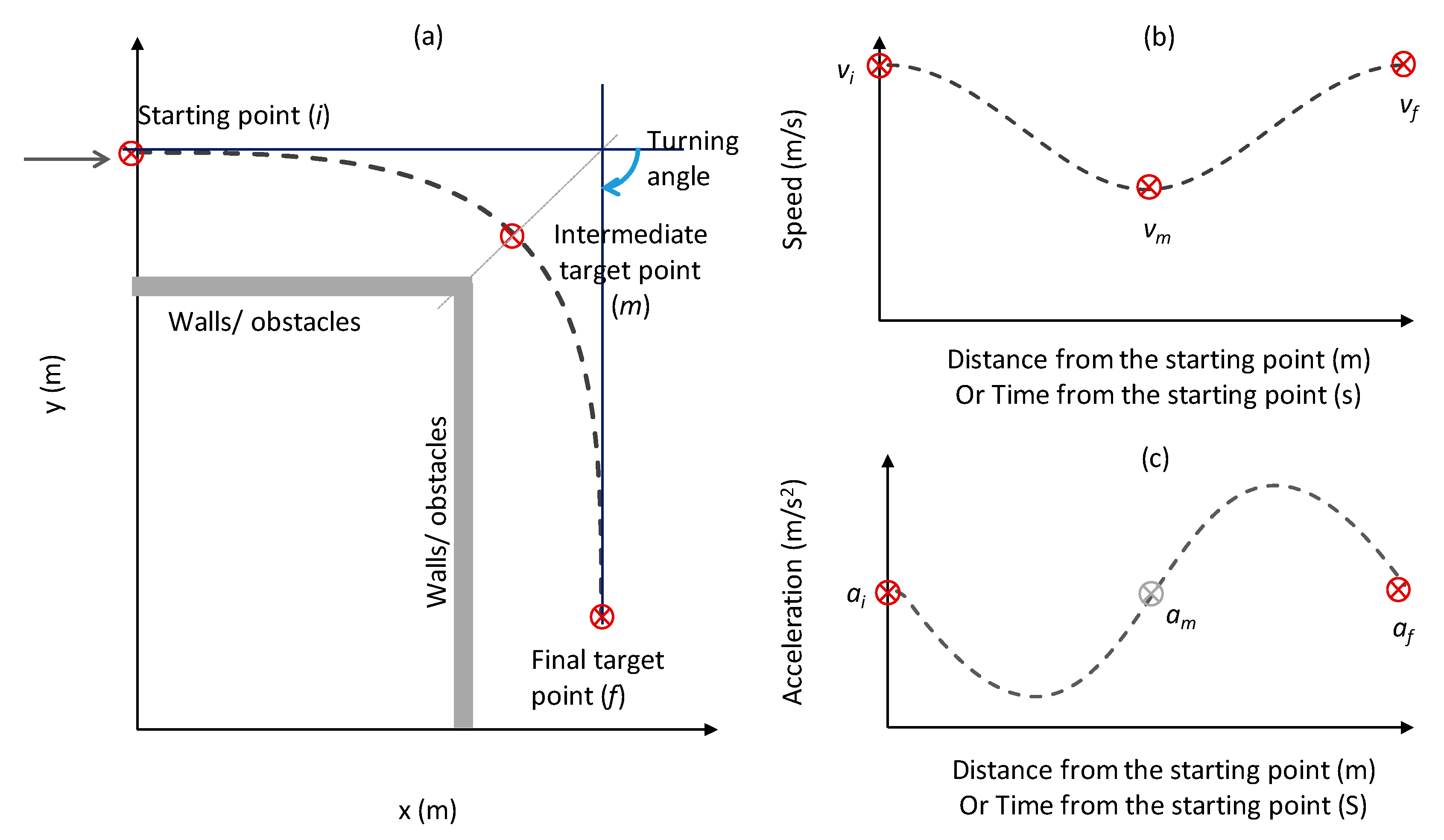
Let us consider a pedestrian is approaching at a bend as schematically shown in Figure 1a. The challenge is to find the path, the speed, and the acceleration profiles (broken lines in Figure 1) that describe the pedestrian’s movement through the corner from the starting point to the final target point.
Before arriving at the corner of the bend, the pedestrian should plan their maneuver through the bend at an upstream point, e.g., at the starting point (i) in Figure 1a. In this study, we considered that pedestrians target an intermediate location (point m in Figure 1a) where their speed drops to a minimum value (vm in Figure 1b). Then, they regain their desired walking speed (vf in Figure 1b) at a final target point (point f in Figure 1a). This assumption is in line with authors’ previous studies that demonstrated that a turning maneuver occurred in a region called the “turning region”, and the turn initiation and end points can be spatially invariant [16]. Other previous studies also experimentally confirmed the spatial invariance of turn initiation points [17,18]. Such points can be considered as starting and final target points. Speeds at those points can be considered as the normal average walking speed of a healthy human with no accelerations or decelerations (i.e., 0 m/s2). Using such assumptions and assuming that the movement time between initial and final target points are known, pedestrians’ turn negotiation maneuvers could be described by the minimum-jerk concept. The minimum-jerk principle describes smoothness in human arm movements [19], and this concept is described in detail in Section 2.2. However, movement time (tf) is generally unknown. If coordinates, speed, and acceleration at an intermediate location are known, such information can be used to obtain an estimate for tf. If we assume that a pedestrian who is planning a turning maneuver is targeting a point on the middle of the corner (Figure 1a), the tangential speed of that point can be estimated based on the instantaneous radius of that point based on the one-thirds power law. The one-thirds power law explains the inverse correlation between the tangential speed and the instantaneous speed as a general feature of human movements. The one-thirds power law is explained in detail in Section 2.3.
2.2. Minimum-Jerk Concept
Flash and Hogan [19] verified that the smoothness of human arm movements such as writing, reaching, and drawing tasks on a plane can be quantified as a function of jerk. As they explained, the objective function for obtaining the smoothest trajectory of a moving hand from a given initial position to a given final position in a given time (tf) is the time integration of the square of jerk, which can be formulated as:
The solution for minimization of Equation (1) can be obtained as a system of fifth order polynomials of time with and (j = {0, …, 5}) constants, as given in Equation (2). Detailed derivations of this system of equation can also be found in [19].
This concept was initially used to describe reaching and catching movements of the human arm in three-dimensional space [20] and goal oriented human movements in two-dimensional space [21]. Further, this concept has been utilized in maneuver planning for autonomous vehicle movements [22] and robot arms movements [23]. Several recent studies applied the minimum-jerk concept to model vehicle speed profiles and maneuvers on expressway curves [24].
2.3. One-Thirds Power Law Concept
The relationship between the radius of the curvature and the tangential speed was empirically studied for handwriting and drawing movements. This relationship can be described with the one-thirds or the two-thirds power laws [25,26,27]. That is, the tangential speed is proportional to the one-third power of the radius of the curvature, or the angular speed is proportional to the two-thirds power of the radius of the curvature. Later, it was empirically proven that this relationship could be valid for human locomotion as well [28,29]. That is, the relationship between walking speed and radius of the curvature of the walking path can be described with power laws. The one-thirds power law relationship can be described as in Equations (3) and (4) as follows:
where V is tangential speed, R is instantaneous radius, and K and are constants.
On a log–log space, tangential speed and radius show a linear relationship [Equation (4)], and the value of approximately equals 0.33 (≈1/3), as experimentally verified in Vieilledent et al. [28]. This relationship describes that the sharper the turn is (i.e., when the radius of the curvature is smaller), the smaller the walking speed at the corner is and vice versa.
2.4. Model Formulation
In the present work, applicability of minimum-jerk and one-thirds power law concepts in combination to estimate pedestrian navigation through bends was explored. These concepts are empirically verified in previous studies as general principles that govern human movements. How such concepts can be used together to model pedestrian movement planning through bends is described in this section.
Dias et al. [16] analyzed trajectories extracted from human experiments and demonstrated that individual pedestrians perform the turning maneuver within a fixed region (described as “turning region”) bounded by “turn initiation” and “turn completion” points. Within this region, there is a deceleration phase followed by an acceleration phase, and the minimum speed occurs approximately at the middle of the corner. Substituting speed and acceleration values at these boundaries of the trajectory, a set of simultaneous equations can be obtained as follows.
At the starting location of the trajectory (i in Figure 1a):
where , , and are the x-components of location, speed, and acceleration at the starting point, respectively. Time was measured from the starting point of the trajectory. The initial location was considered as the turn initiation point, and the coordinates of that point were set as (0, 0). Approaching speed at the turn initiation point was set as the free flow walking speed, which is known. The acceleration at initial point was considered as 0 m/s2.
At the final target point of the trajectory (i.e., f in Figure 1a):
where , , and are the x-components of location, speed, and acceleration at the final location or the exit point, respectively. The final location was considered as the turn completion point. The coordinates of that point for each turning angle case were set relative to the origin based on the corridor geometry and the dimensions of the turning region. Receding or exit speed at the turn completion point was also set as the free-flow walking. The acceleration at final point or exit point was also considered as 0 m/s2.
As the minimum speed occurs approximately at the middle of the corner, if the coordinates, the speed, and the acceleration at such point is known, the following equations can be obtained:
where is time to the intermediate target point (i.e., m in Figure 1a) measured from the starting point, and , , and are the x-components of location, speed, and acceleration at the location of minimum speed, respectively. As described earlier (in Figure 1), it is reasonable to assume that people are planning their movement via the middle point of the corner and keeping a certain safe distance from the inner corner of the bend. If the instantaneous radius on the trajectory at that point is known, the speed at that point can be obtained based on the power law relationship [Equation (3)].
By considering Equations (5)–(7), it can be noted that there are eight unknowns (, , , , , , , and ) with eight simultaneous equations (i.e., ignoring the last equation of (7)). Thus, a set of solutions can be obtained for constants and movement times. Once an estimate for is obtained, constants for the y-components of the trajectory (, , , , , and ) can also be obtained by solving the following set of equations.
At the starting location of the trajectory:
where , , and are the y-components of location, speed, and acceleration at the starting point, respectively. These are as described earlier.
At the final location of the trajectory:
where , , and are the y-components of location, speed, and acceleration at the final target point, respectively.
The simultaneous equations were solved for 90°, 135°, and 180° turnings separately, and outputs were compared with empirical trajectories. Details of the model verification are discussed in the following section.
3. Model Verification
In this study, trajectory data collected through a controlled experiment conducted at Monash University, Australia in 2013 [16] were used to verify the model. This experiment was conducted to understand solo pedestrian walking characteristics through different turning configurations. Sixteen postgraduate students (11 males and five females) participated in this experiment, and their ages ranged from 26 to 33 years. Corridors (width = 1.5 m) of different angles (45°, 60°, 90°, 135°, and 180°) were set out using safety barriers, chains, and tapes. Therefore, the downstream conditions beyond the turning point were visible. Three desired speed levels were considered (normal-speed walking, fast-speed walking, and slow-speed running), and the data for normal speed walking through 90°, 135°, and 180° corridors were used in this study. Before the normal speed walking scenarios, participants were instructed to walk through the corridor at their normal walking speed. We did not ask participants to follow a specific path, and they were allowed to walk freely through the corridor. The purpose of the experiment was not revealed to the participants. Experiments were video recorded with an overhead video camera, and positions of participants’ heads were obtained at 0.24 s intervals by manual tracking.
In order to solve the above formulated simultaneous equations for different turning angles, coordinates of the initial and the final points were obtained based on the corridor geometry (width = 1.5 m) and the dimensions of the turning region provided in Dias et al. [16]. To estimate the speed at the intermediate point using the power law relationship, the instantaneous radius of that point was required. The method adopted in this study to obtain an estimate for the instantaneous radius is described in Section 3.1.
3.1. Estimating Instantaneous Radius of the Path
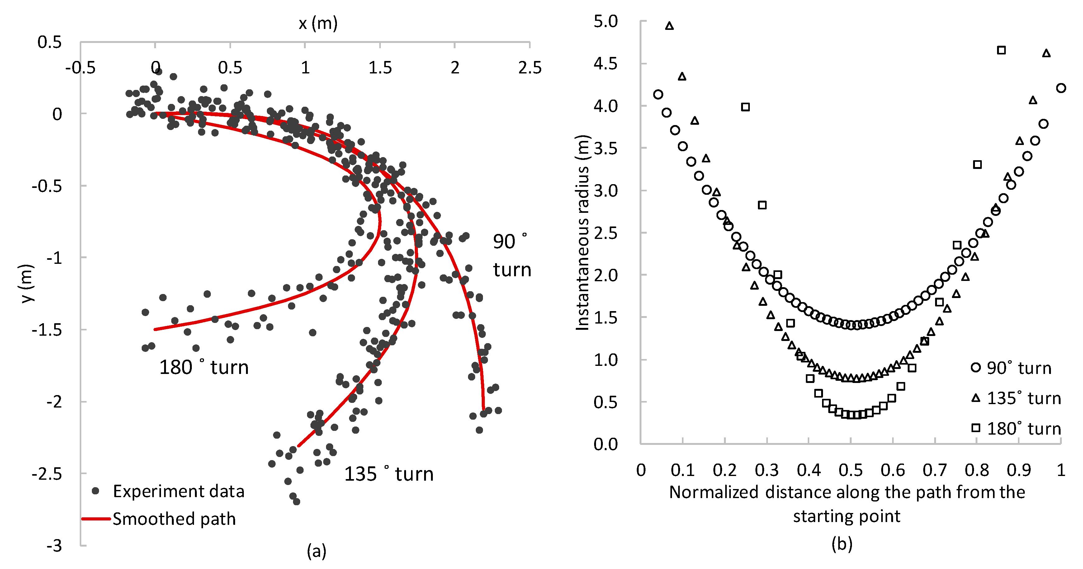
In order to obtain an approximate estimate for the instantaneous radius at the intermediate point, fourth order polynomials on x-y space were considered, which were fitted based on several paths obtained from experimental trajectories. It should be noted that it is possible to obtain a higher order polynomial that passes through initial, intermediate, and final points considering location as well as tangent information at these points, even without empirical data. The following formula was used to calculate the instantaneous radius (R) of the path, which is described by a fourth order polynomial (y = f(x)) on x-y space:
Fitted polynomials and estimated instantaneous radii for 90°, 135°, and 180° turning cases are illustrated in Figure 2.
It can be noted that the minimum radius was located approximately at the middle of the trajectory, i.e., when the normalized distance was approximately 0.5. It could further be observed that the minimum radius was generally smaller for higher degree turns or sharp turns compared to smaller degree turns. When the instantaneous radius at the intermediate point, which could be considered as the minimum radius, was known, instantaneous speed at the point could be estimated using the power law relationship, as discussed in the following subsection.
3.2. Power Law Parameters
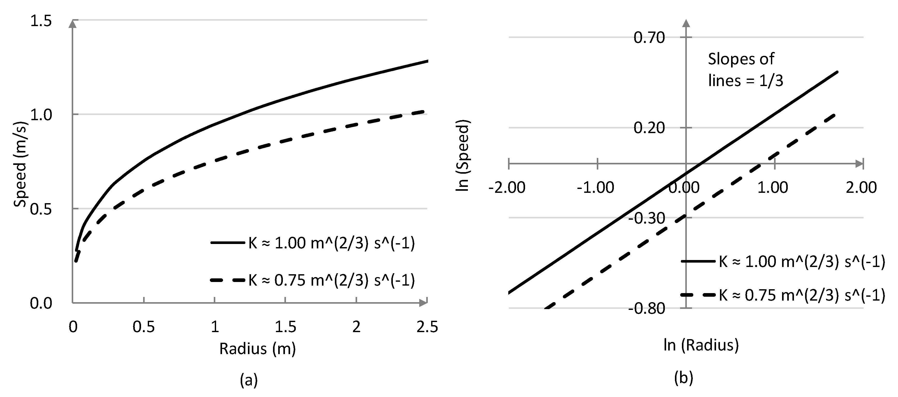
The relationship between radius and speed [Equations (3) and (4)] for different K values calibrated in Vieilledent et al. [28] using empirical data are shown in Figure 3. It is clear that, for a given radius, speed could be significantly varied based on the value of K. It should be noted that the approximate ranges of radii in the experiment by Vieilledent et al. [28] were 2 m, (0.5, 3) m, and (0.2, 13.5) m for K = 1.75, 1.0, and 0.75 m(2/3)s−1 (approximately), respectively. In this study, the instantaneous radii at the intermediate point were varied approximately between 0.5 m and 2 m. Thus, K = 1.00 m(2/3) s−1 was used in this study to estimate speeds at the intermediate point.
Based on such settings, a Monte Carlo simulation was conducted to generate trajectories. Resulting trajectories were compared with empirical trajectories, and details are described in the following section.
3.3. Results
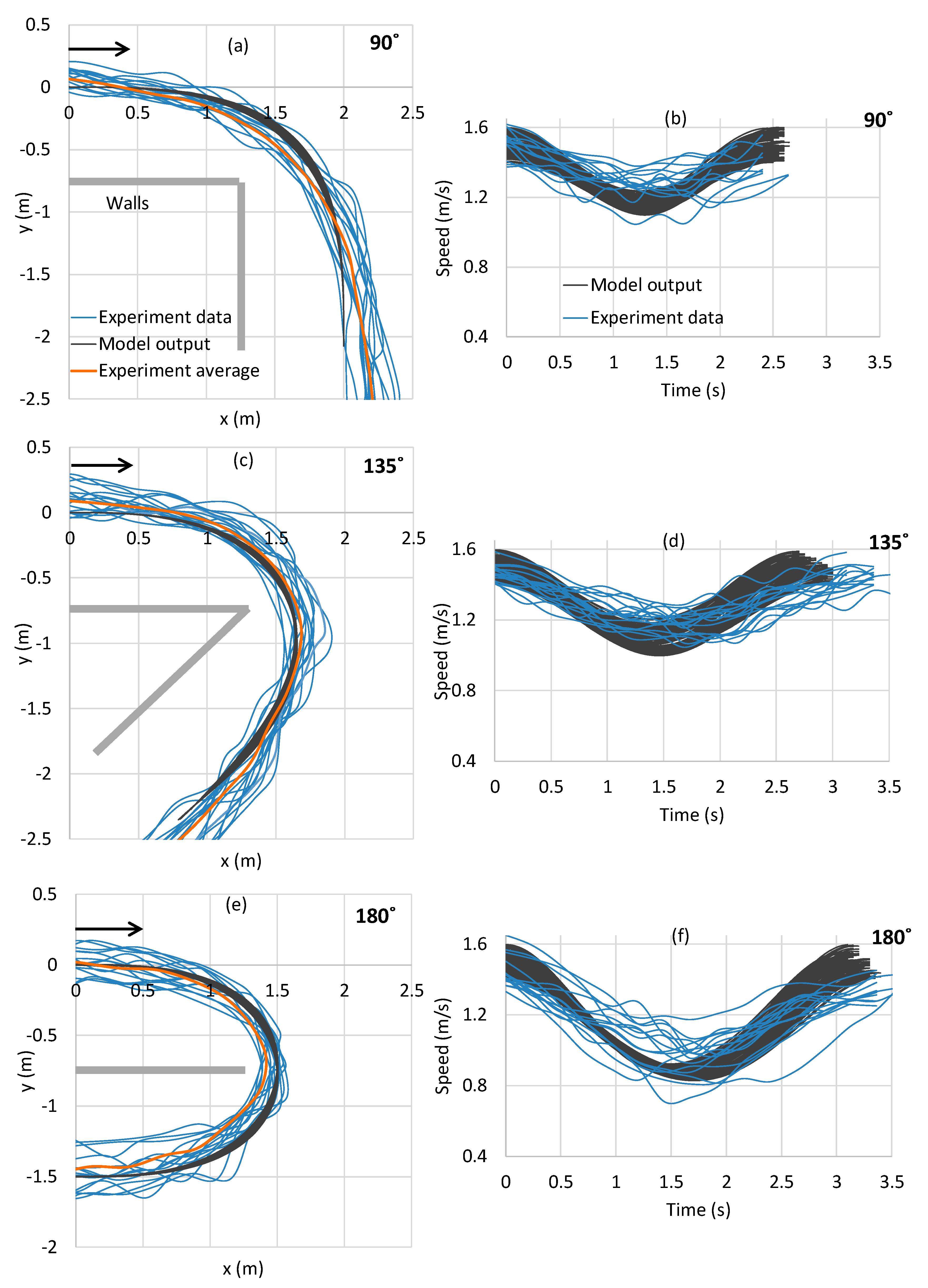
In the simulation, the starting, the intermediate, and the final locations were set based on the dimensions of the turning regions for 90°, 135°, and 180° turning angles. Speeds at the starting and the final locations were assumed to be distributed uniformly between 1.4 m/s and 1.6 m/s as the free flow speeds of empirical data were also distributed approximately in this range. i.e., at each simulation, two speed values were randomly chosen from these distributions as speeds at initial and final locations. Speeds at the intermediate location were estimated based on the power law relationship. Assuming that the deceleration and the acceleration phases occurred within the turning region, accelerations at the starting and the final locations were set as 0 m/s2. A Monte Carlo simulation was conducted with 100 random seeds, and the outputs, i.e., paths, speed, and acceleration profiles, for 90°, 135°, and 180° turning angles were compared with empirical data, as shown in Figure 4.
It can be noted that, although the speeds at the intermediate location were set as a fixed value for each turning angle case, a range of minimum speed values resulted. This was mainly because we used the values resulting from Equations (5)–(7) (i.e., solving the simultaneous equations for x-direction) to estimate coefficients for both x- and y-directions or vice-versa. The range of tf values resulted because of the range of vi and vf values used in simultaneous equations.
The simultaneous equations provided multiple sets of solutions. In this study, eight sets of solutions were obtained for each case, i.e., four real and four complex solutions. Out of the four real solutions, two were unrealistic (i.e., tf or tm < 0). Thus, the global minimum was carefully chosen by setting appropriate initial values.
For a given turning angle, no remarkable variation was observed in simulated paths even though the speeds at the entry and the exit points were different. Regarding speed profiles, the variations could be acceptable, as empirical speed profiles were also varied in more or less a similar manner. Further, in order to obtain minimum-jerk trajectories, i.e., to solve Equation (2), only tf was required in addition to location, speed, and acceleration vectors at initial and final locations. Thus, at this stage, we used the location and the speed information at the intermediate location only for the estimation of tf.
The developed combined model generates pedestrian walking trajectories (path, speed, and acceleration profile) considering the physical boundaries of the corner. It does not require empirical calibration or adjustment. It only requires the characteristics of entry and exit points (location, speed, and acceleration). The presented simulated trajectories in Figure 4 assume one entry and one exit point. In the experimental data, participants chose different entry and exit points. This is clearly shown in Figure 4a,c,e. Simulated paths fit well within the range of observed paths, which supports the reliability of the minimum-jerk and the power law integrated model in presenting human walking maneuvers around corners. Maximum deviations of the modeled paths from the average of empirical paths were estimated as 0.16 m, 0.08 m, and 0.14 m for 90°, 135°, and 180° turning cases, respectively. The variance of simulated paths was smaller compared to empirical ones, mainly because of the variance in initial, intermediate, and final locations. In this study, we did not consider such variances, as the purpose was to model humans’ movement planning around bends via three given points.
Minimum speeds (±standard deviation) for the modeled trajectories were 1.16 (±0.03) m/s, 1.09 (±0.06) m/s, and 0.88 (±0.02) m/s for 90°, 135°, and 180° turnings, respectively. For empirical data, minimum speeds were 1.24 (±0.09) m/s, 1.16 (±0.07) m/s, and 0.93 (±0.11) m/s for 90°, 135°, and 180° turnings, respectively. It can be noted that the model underestimated the minimum speed or the speed at the intermediate point. The Mann–Whitney U test [30] confirmed that, for all turning angles, the differences between medians of the minimum speeds were statistically significant. Results of the Mann–Whitney U test for 90°, 135°, and 180° were (z-score = 3.80, p-value = 0.00014), (z-score = 3.37, p-value = 0.00076), and (z-score = 2.45, p-value = 0.0143), respectively. This could possibly be attributed to the default power law parameters (calibrated in [28]) used in this study. Experiment conditions could be remarkably different in these two cases. Furthermore, the experiment by Vieilledent et al. [28] considered walking on differently shaped paths, which were mainly circular and elliptical shaped paths, and those were not exactly similar to the turning maneuvers considered in this study. Nevertheless, with a proper recalibration of power law principle, the proposed model in this study can further be improved to obtain a better estimate for speed profiles as well.
4. Sensitivity Analysis
Sensitivity of the proposed modeling approach for different initial, intermediate, and exit conditions was also investigated, and results are summarized in this section.
4.1. Entry and Exit Acceleration
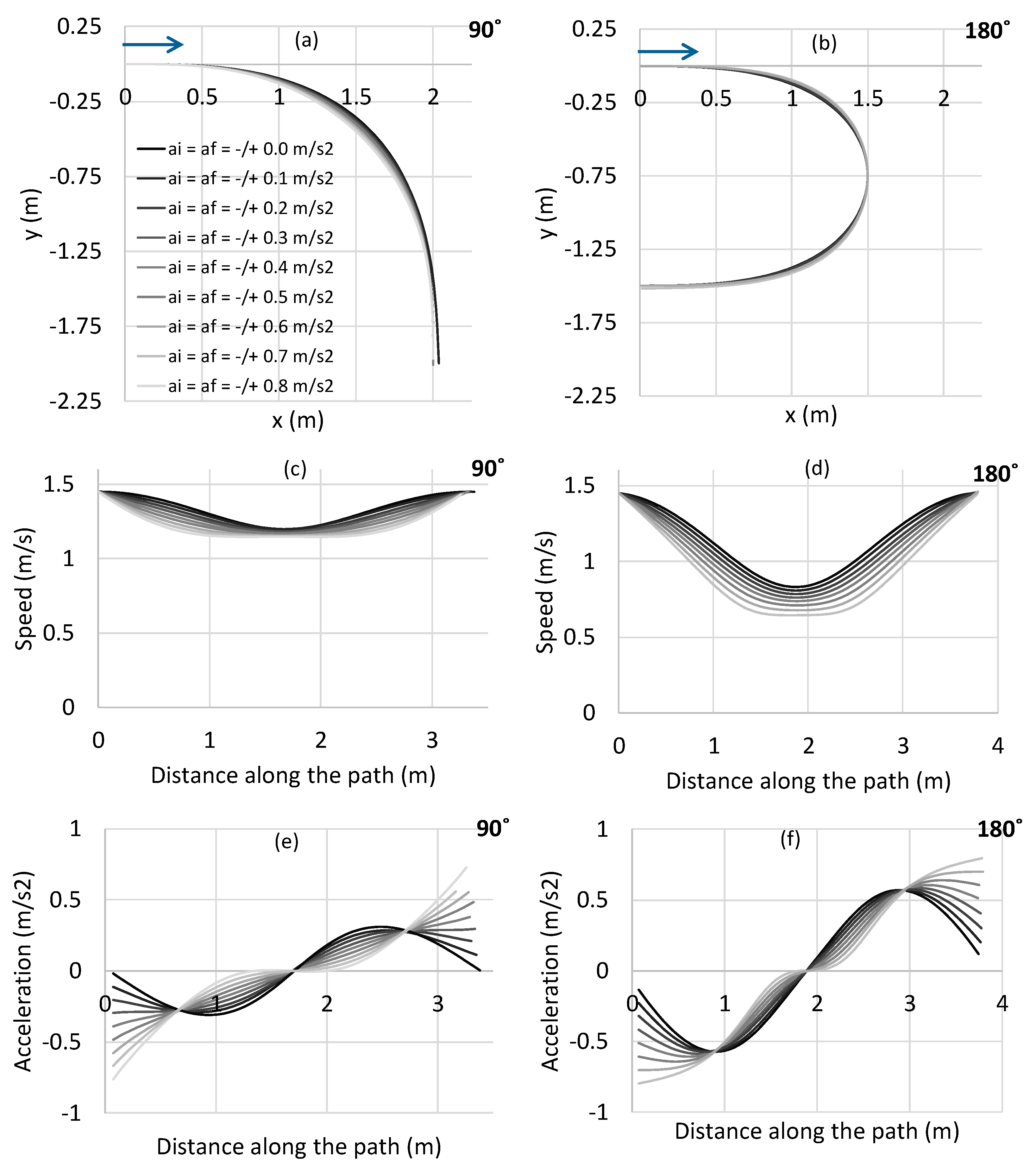
It was assumed in the previous section that the deceleration and the acceleration phases occurred within the initial and the final locations (i.e., within the turning region). However, this is not always the case, and there could be variations in the dimensions of the turning region. Effects of deceleration and acceleration at initial and final locations, respectively, on the variation of estimated trajectories were also explored, and the results are summarized in this subsection.
In the simulation, speeds at initial and final locations were set as 1.45 m/s, which is approximately the average free flow walking speed. Speeds at the intermediate locations were estimated based on the power law relationship and the instantaneous radii estimated using fourth order polynomial traverses through initial, intermediate, and final points. Magnitudes of the entry deceleration and the exit acceleration were considered to be similar. Trajectories were simulated for different entry and exit accelerations ranging from 0 m/s2 to 0.8 m/s2. Resulting trajectories for 90° and 180° turning cases are shown in Figure 5.
It could be observed that, for a given turning angle, paths were not remarkably varied from each other. However, significant variations were observed in speed and acceleration profiles. That is, speed and acceleration profiles during the whole movement were dependent on the initial and the final acceleration values. These observations indicate that individuals mainly adjust speed and accelerations only (i.e., keeping similar walking paths) to traverse through a bend.
4.2. Exit Location
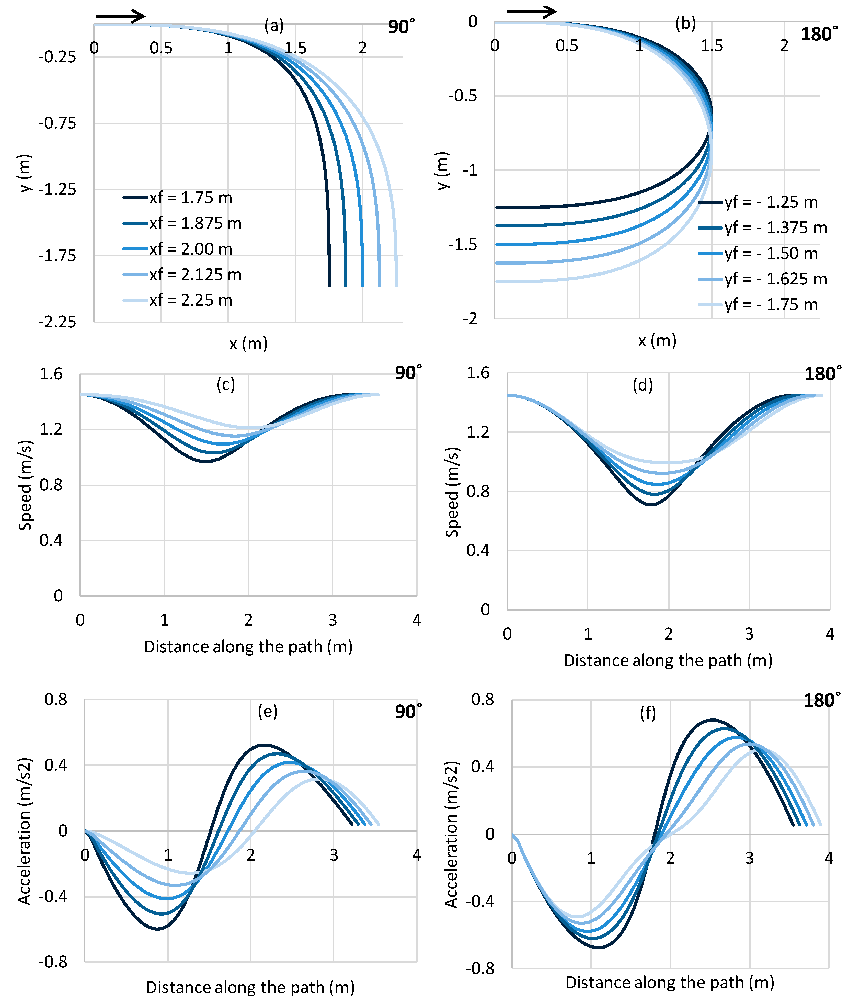
Although an individual plans a movement at an initial point via an intermediate point, there could be different final or exit points. How trajectories are varied depending on the final location was also investigated. In these simulations, speeds at initial and final locations were set as 1.45 m/s. Speeds at the intermediate locations were estimated based on the power law relationship considering instantaneous radius of the path of the base case (i.e., xf = 2.00 m for 90° case and yf = −1.50 m for 180° case). Accelerations at initial and final locations were set as 0 m/s2. Based on such settings, simultaneous equations were solved for the same entry location but for a range of different exit locations. Resulting trajectories are shown in Figure 6.
It could be observed that, even though fixed speed values (for 90° and 180° cases separately) were set at the intermediate points, a range of minimum speed values resulted. This was rational and was attributed to the same reason as described in Section 3.3, i.e., the use of the values resulting from Equations (5)–(7) to estimate coefficients for both x- and y-directions or vice-versa. Obviously, different values are possible for different xf and yf. Nevertheless, the results obtained here are logical. The smaller the minimum radius of the path is, the smaller the minimum speed at the intermediate location will be.
4.3. Radius of the Walking Path
Even though the turning angle is the same, the minimum radius of the path could be significantly different. How the trajectories varied for different radii for the same turning angle is evaluated in this section.
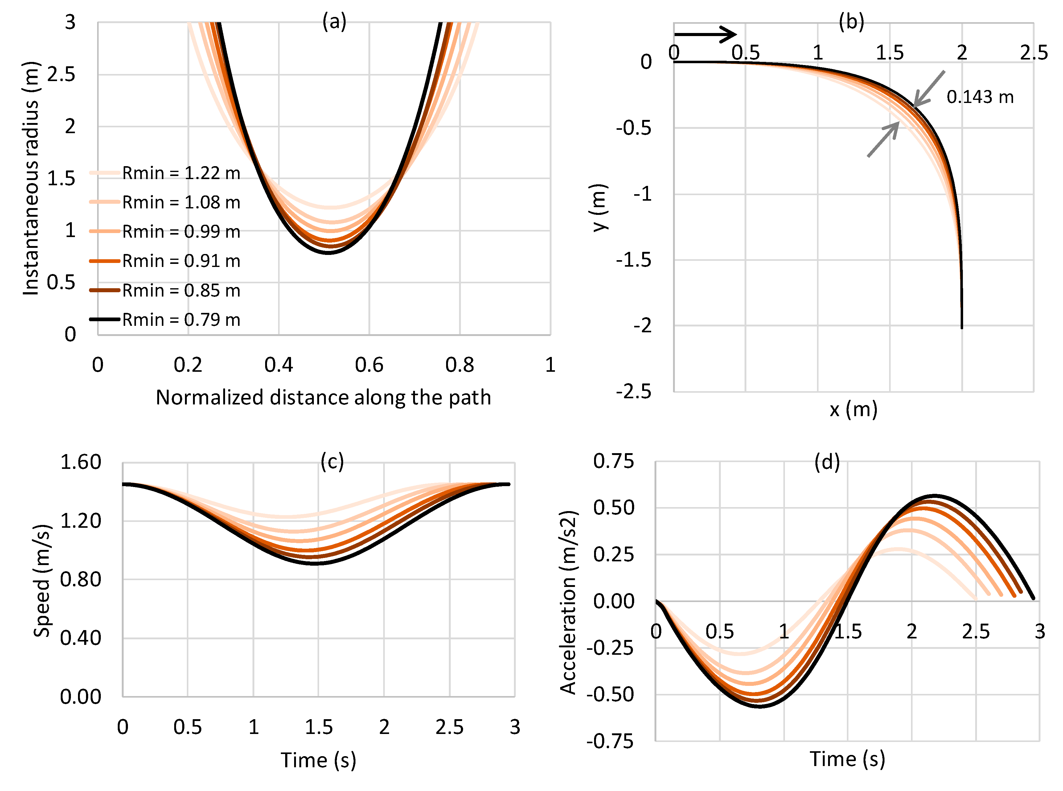
For the simulation, different intermediate points were assumed for fixed initial and final locations. Instantaneous radii were estimated using a fourth order polynomials traverse through initial, intermediate, and final locations (Figure 7a). Speed at the intermediate location was set based on the power law relationship. Entry and exit speeds were assumed to be similar and were set as 1.45 m/s. Accelerations at entry and exit locations were set as 0 m/s2. Resulting paths, speed, and acceleration profiles for 90° turning are compared in Figure 7b–d, respectively.
It could be observed that, even though paths were not considerably deviated (0.143 m), speed and acceleration profiles displayed a significant variation due to the differences in minimum radii at the intermediate point. Minimum speeds varied between 0.91 m/s and 1.22 m/s, and magnitudes of maximum accelerations (or minimum deceleration) varied between 0.28 m/s2 and 0.56 m/s2.
It could further be observed that the movement time increased when a person moved further away from the bend at the inner corner. That is, the shortest path was achieved when a person walked closer to the inner wall. Such logical behaviors could also be realistically captured in the proposed model.
5. Conclusions and Further Studies
Information regarding trajectories of pedestrians’ turning maneuvers can be used in many applications, such as in microscopic simulations, motion planning of autonomous agents, and visualization of movements in VR and DS applications. This study investigated the applicability of minimum-jerk and one-thirds power law concepts in movement planning of pedestrians when negotiating bends. The comparison of modeled and observed actual paths explained that the proposed approach could reproduce walking paths with good accuracy. Although speed and acceleration patterns were accurately reproduced, it was noted that the model underestimated the minimum speed for all bends. This was mainly due to the use of default parameter K of the power law equation that was calibrated in previous studies under different experimental conditions. Further, due to the large variation in K values of the power law relationship calibrated in previous studies, it was hard to define a proper value in this study. Thus, further empirical investigations are necessary to recalibrate the parameter K considering various factors, e.g., demographic characteristics, affecting walking speed of pedestrians.
Sensitivity analysis explained that the model could logically respond to the changes in initial, intermediate, and final conditions and realistically reproduce paths, speed, and acceleration profiles. That is, the model could be applied in estimating trajectories of humans negotiating bends under different initial and target conditions. Nevertheless, additional experimental data, particularly for different boundary conditions and walking radii, are required to further validate these findings.
Instantaneous radius of the walking path is an input for the model presented in this study, and the accuracy of the speed at the intermediate location depends on the accuracy of the estimated instantaneous radii. In this study, for the sake of simplicity, a fourth order polynomial that passed through initial, final, and intermediate locations was considered to estimate instantaneous radii. Other methods such as spline or clothoid curves may also be used considering the tradeoff between accuracy of the estimates and the computational costs.
In this study, only the solo turning cases, which can be considered as the base movement pattern in any microscopic simulation or movement planning application, were modeled. Further studies are necessary to evaluate the deviation between the planned or the desired path (under solo conditions) and the resulting path in the presence of obstacles, such as interacting pedestrians.
Author Contributions
Conceptualization, C.D.; Methodology, C.D. and M.A.; Software, M.A.; Validation, M.A. and C.D.; Formal Analysis, C.D., M.A. and R.L.; Data Curation, C.D. and M.S.; Writing–Original Draft Preparation, C.D. and M.A.; Writing–Review & Editing, C.D., R.L. and W.A.; Supervision, M.S.
Funding
This research received no external funding.
Acknowledgments
The publication of this article was funded by the Qatar National Library.
Conflicts of Interest
The authors declare no conflict of interest.
References
- Sedgman, R.; Goldie, P.; Iansek, R. Development of a measure of turning during walking. In Proceedings of the Advancing Rehabilitation: Inaugural Conference of the Faculty of Health Sciences, Bundoora, Australia, 2–4 November 1994. [Google Scholar]
- Morris, M.E.; Huxham, F.; McGinley, J.; Dodd, K.; Iansek, R. The biomechanics and motor control of gait in Parkinson disease. Clin. Biomech. 2001, 16, 459–470. [Google Scholar] [CrossRef]
- Odonkor, C.A.; Thomas, J.C.; Holt, N.; Latham, N.; Van Swearingen, J.; Brach, J.S.; Leveille, S.G.; Jette, A.; Bean, J. A comparison of straight-and curved-path walking tests among mobility-limited older adults. J. Gerontol. A Biomed. Sci. Med. Sci. 2013, 68, 1532–1539. [Google Scholar] [CrossRef] [PubMed]
- Patla, A.E.; Prentice, S.D.; Robinson, C.; Neufeld, J. Visual control of locomotion: Strategies for changing direction and for going over obstacles. J. Exp. Psychol. Hum. Percept. Perform. 1991, 17, 603. [Google Scholar] [CrossRef] [PubMed]
- Hase, K.; Stein, R.B. Turning strategies during human walking. J. Neurophysiol. 1999, 81, 2914–2922. [Google Scholar] [CrossRef] [PubMed]
- Taylor, M.J.; Dabnichki, P.; Strike, S.C. A three-dimensional biomechanical comparison between turning strategies during the stance phase of walking. Hum. Mov. Sci. 2005, 24, 558–573. [Google Scholar] [CrossRef] [PubMed]
- Courtine, G.; Schieppati, M. Human walking along a curved path. II. Gait features and EMG patterns. Eur. J. Neurosci. 2003, 18, 191–205. [Google Scholar] [CrossRef]
- Akiyama, Y.; Okamoto, S.; Toda, H.; Ogura, T.; Yamada, Y. Gait motion for naturally curving variously shaped corners. Adv. Robot. 2018, 32, 77–88. [Google Scholar] [CrossRef]
- Shiwakoti, N.; Sarvi, M.; Rose, G.; Burd, M. Consequence of turning movements in pedestrian crowds during emergency egress. Transp. Res. Rec. J. Transp. Res. Board 2011, 2234, 97–104. [Google Scholar] [CrossRef]
- Dias, C.; Sarvi, M.; Shiwakoti, N.; Ejtemai, O.; Burd, M. Investigating collective escape behaviours in complex situations. Saf. Sci. 2013, 60, 87–94. [Google Scholar] [CrossRef]
- Kretz, T. The use of dynamic distance potential fields for pedestrian flow around corners. In Proceedings of the First International Conference on Evacuation Modeling and Management (ICEM 09), TU Delft, The Netherlands, 23–25 September 2009. [Google Scholar]
- Guo, R.Y.; Tang, T.Q. A simulation model for pedestrian flow through walkways with corners. Simul. Model. Pract. Theory 2012, 21, 103–113. [Google Scholar] [CrossRef]
- Dias, C.; Ejtemai, O.; Sarvi, M.; Burd, M. Exploring pedestrian walking through angled corridors. Transp. Res. Procedia 2014, 2, 19–25. [Google Scholar] [CrossRef]
- Li, S.; Li, X.; Qu, Y.; Jia, B. Block-based floor field model for pedestrian’s walking through corner. Phys. A Stat. Mech. Appl. 2015, 432, 337–353. [Google Scholar] [CrossRef]
- Dias, C.; Lovreglio, R. Calibrating cellular automaton models for pedestrians walking through corners. Phys. Lett. A 2018, 382, 1255–1261. [Google Scholar] [CrossRef]
- Dias, C.; Ejtemai, O.; Sarvi, M.; Shiwakoti, N. Pedestrian walking characteristics through angled corridors: An experimental study. Transp. Res. Rec. J. Transp. Res. Board 2014, 2421, 41–50. [Google Scholar] [CrossRef]
- Grasso, R.; Ivanenko, Y.P.; McIntyre, J.; Viaud-Delmon, I.; Berthoz, A. Spatial, not temporal cues drive predictive orienting movements during navigation: A virtual reality study. Neuroreport 2000, 11, 775–778. [Google Scholar] [CrossRef]
- Prévost, P.; Yuri, I.; Renato, G.; Alain, B. Spatial invariance in anticipatory orienting behaviour during human navigation. Neurosci. Lett. 2003, 339, 243–247. [Google Scholar] [CrossRef]
- Flash, T.; Hogan, N. The coordination of arm movements: An experimentally confirmed mathematical model. J. Neurosci. 1985, 5, 1688–1703. [Google Scholar] [CrossRef]
- Bratt, M.; Smith, C.; Christensen, H.I. Minimum jerk based prediction of user actions for a ball catching task. In Proceedings of the 2007 IEEE/RSJ International Conference on Intelligent Robots and Systems, San Diego, CA, USA, 29 October–2 November 2007; pp. 2710–2716. [Google Scholar]
- Pham, Q.C.; Hicheur, H.; Arechavaleta, G.; Laumond, J.P.; Berthoz, A. The formation of trajectories during goal-oriented locomotion in humans. II. A maximum smoothness model. Eur. J. Neurosci. 2007, 26, 2391–2403. [Google Scholar] [CrossRef]
- Shamir, T. How should an autonomous vehicle overtake a slower moving vehicle: Design and analysis of an optimal trajectory. IEEE Trans. Autom. Control 2004, 49, 607–610. [Google Scholar] [CrossRef]
- Wada, Y.; Kawato, M. A via-point time optimization algorithm for complex sequential trajectory formation. Neural Netw. 2004, 17, 353–364. [Google Scholar] [CrossRef]
- Dias, C.; Oguchi, T.; Wimalasena, K. Drivers’ Speeding Behavior on Expressway Curves: Exploring the Effect of Curve Radius and Desired Speed. Transp. Res. Rec. 2018, 2672, 48–60. [Google Scholar] [CrossRef]
- Lacquaniti, F.; Terzuolo, C.; Viviani, P. The law relating the kinematic and figural aspects of drawing movements. Acta Psychol. 1983, 54, 115–130. [Google Scholar] [CrossRef]
- Viviani, P.; Schneider, R. A developmental study of the relationship between geometry and kinematics in drawing movements. J. Exp. Psychol. Hum. Percept. Perform. 1991, 17, 198. [Google Scholar] [CrossRef] [PubMed]
- Gribble, P.L.; Ostry, D.J. Origins of the power law relation between movement velocity and curvature: Modeling the effects of muscle mechanics and limb dynamics. J. Neurophysiol. 1996, 76, 2853–2860. [Google Scholar] [CrossRef] [PubMed]
- Vieilledent, S.; Kerlirzin, Y.; Dalbera, S.; Berthoz, A. Relationship between velocity and curvature of a human locomotor trajectory. Neurosci. Lett. 2001, 305, 65–69. [Google Scholar] [CrossRef]
- Hicheur, H.; Vieilledent, S.; Richardson, M.J.E.; Flash, T.; Berthoz, A. Velocity and curvature in human locomotion along complex curved paths: A comparison with hand movements. Exp. Brain Res. 2005, 162, 145–154. [Google Scholar] [CrossRef] [PubMed]
- Fay, M.P.; Proschan, M.A. Wilcoxon-Mann-Whitney or t-test? On assumptions for hypothesis tests and multiple interpretations of decision rules. Stat. Surv. 2010, 4, 1–39. [Google Scholar] [CrossRef]
Figure 1.
Maneuver planning around a corner: (a) path; (b) speed profile; (c) acceleration profile.

Figure 2.
(a) Smoothed paths with fourth order polynomials; (b) Estimated instantaneous radii along the path.
Figure 2.
(a) Smoothed paths with fourth order polynomials; (b) Estimated instantaneous radii along the path.

Figure 3.
Sensitivity of the power law relationship for different K on; (a) x-y space; (b) ln(x)-ln(y) space.
Figure 3.
Sensitivity of the power law relationship for different K on; (a) x-y space; (b) ln(x)-ln(y) space.

Figure 4.
Comparison of model outputs with experiment data: (a) paths for 90° turning; (b) speed profiles for 90° turning; (c) paths for 135° turning; (d) speed profiles for 135° turning; (e) paths for 180° turning; (f) speed profiles for 180° turning.
Figure 4.
Comparison of model outputs with experiment data: (a) paths for 90° turning; (b) speed profiles for 90° turning; (c) paths for 135° turning; (d) speed profiles for 135° turning; (e) paths for 180° turning; (f) speed profiles for 180° turning.

Figure 5.
Sensitivity of the model to the entry and the exit accelerations: (a) paths for 90° turning; (b) paths for 180° turning; (c) speed profiles for 90° turning; (d) speed profiles for 180° turning; (e) acceleration profiles for 90° turning; (f) acceleration profiles for 180° turning.
Figure 5.
Sensitivity of the model to the entry and the exit accelerations: (a) paths for 90° turning; (b) paths for 180° turning; (c) speed profiles for 90° turning; (d) speed profiles for 180° turning; (e) acceleration profiles for 90° turning; (f) acceleration profiles for 180° turning.

Figure 6.
Sensitivity of the model to the exit location: (a) paths for 90° turning; (b) paths for 180° turning; (c) speed profiles for 90° turning; (d) speed profiles for 180° turning; (e) acceleration profiles for 90° turning; (f) acceleration profiles for 180° turning.
Figure 6.
Sensitivity of the model to the exit location: (a) paths for 90° turning; (b) paths for 180° turning; (c) speed profiles for 90° turning; (d) speed profiles for 180° turning; (e) acceleration profiles for 90° turning; (f) acceleration profiles for 180° turning.

Figure 7.
(a)-Estimated instantaneous radii along paths; (b) comparison of paths; (c) comparison of speed profiles; (d) comparison of acceleration profiles.
Figure 7.
(a)-Estimated instantaneous radii along paths; (b) comparison of paths; (c) comparison of speed profiles; (d) comparison of acceleration profiles.

© 2019 by the authors. Licensee MDPI, Basel, Switzerland. This article is an open access article distributed under the terms and conditions of the Creative Commons Attribution (CC BY) license (http://creativecommons.org/licenses/by/4.0/).
Share and Cite
MDPI and ACS Style
Dias, C.; Abdullah, M.; Sarvi, M.; Lovreglio, R.; Alhajyaseen, W. Modeling and Simulation of Pedestrian Movement Planning Around Corners. Sustainability 2019, 11, 5501. https://doi.org/10.3390/su11195501
AMA Style
Dias C, Abdullah M, Sarvi M, Lovreglio R, Alhajyaseen W. Modeling and Simulation of Pedestrian Movement Planning Around Corners. Sustainability. 2019; 11(19):5501. https://doi.org/10.3390/su11195501
Chicago/Turabian StyleDias, Charitha, Muhammad Abdullah, Majid Sarvi, Ruggiero Lovreglio, and Wael Alhajyaseen. 2019. "Modeling and Simulation of Pedestrian Movement Planning Around Corners" Sustainability 11, no. 19: 5501. https://doi.org/10.3390/su11195501
Note that from the first issue of 2016, this journal uses article numbers instead of page numbers. See further details here.