Empirical Detection and Quantification of Price Transmission in Endogenously Unstable Markets: The Case of the Global–Domestic Coffee Supply Chain in Papua New Guinea

Abstract

Price transmission through global–domestic agricultural supply chains is a fundamental indicator of domestic market efficiency and producer welfare. Conventional price-transmission econometrics test for a theory-based spatial-arbitrage restriction that long-run equilibrium prices in spatially distinct markets differ by no more than transaction costs. The conventional approach is ill-equipped to test for price transmission when endogenously unstable markets do not equilibrate due to systematic arbitrage-frustrating frictions including financial and institutional transaction costs and biophysical constraints. We propose a novel empirical framework using price data to test for market stability and price transmission along international-domestic supply chains incorporating nonlinear time series analysis and recently emerging causal-detection methods from empirical nonlinear dynamics. We apply the framework to map-out and quantify price transmission through the global-exporter–processor–producer coffee supply chain in Papua, New Guinea. We find empirical evidence of upstream price transmission from the global market to domestic exporters and processors, but not through to producers.

1. Introduction

Price transmission concerns the extent to which price changes from one market pass through to spatially distinct markets, and consequently, is a fundamental indicator of market integration along global–domestic supply chains, domestic market efficiency, and economic welfare of exporters, processors, and producers [1]. Price transmission is also a fundamental indicator of the economic sustainability of regional supply chains and the social sustainability of domestic participants. The Brundtland Commission (1987) defined sustainability as “development that meets the needs of the present without compromising the ability of future generations to meet their own needs” [2]. Arrow et al. (2004) took this to mean that “intertemporal social welfare must not decrease over time” [3]. In this context, policymakers rely on “before-and-after” measures of price transmission to empirically determine whether global trade policies have had an adverse welfare impact on domestic markets [1]. For price transmission to be a reliable welfare measure, there is critical need for theory and empirical practice to correspond to real-world global–domestic supply-chain price dynamics.

1.1. Past Work

The theory of price transmission, given by the Law of One Price, holds that equilibrium (e) prices of the same commodity in distinct markets will differ by market transactions costs (tc): $p_1^e-p_2^e=tc$. A spatial-arbitrage condition restricts $p_1^e \mathrm{and} p_2^e$ to be stable in the face of external random market shocks. Driven by forces of supply and demand, markets self-correct so that, at each point in time, re-equilibrating prices differ at most by transactions costs: $p_{1t}-p_{2t}\le tc$. Complete price transmission occurs when prices have re-equilibrated; however, transmission remains incomplete during an adjustment period whose length depends on the speed of adjustment [4].

Early empirical practice, based on linear time series analysis, detected price transmission by testing temporal price series data for cointegration; simply put, price co-movement through time driven by the spatial-arbitrage condition. Cointegration is the gateway to analysis [5]: First, cointegrated prices are Granger-causally interactive in at least one direction. Granger-causality testing must be subsequently done to determine the directions. Second, cointegrated prices are amenable to an error correction model (ECM) specification, which allows computation of the completeness and speed of price transmission as self-correcting markets adjust to long-run equilibrium.

Empirical practice reached a threshold as recognition grew that key factors—especially asymmetric price response and high transactions costs—could inhibit spatial arbitrage in real-world markets, and that modeling this behavior was beyond the reach of conventional linear cointegration analysis [1,6]. Asymmetric price response occurs when the rate of transmission abruptly shifts around some factor; for example, global prices. Intermediate entities in the supply chain (e.g., wholesalers) with market power over price may adopt strategies resulting in incomplete and slow price transmission to upstream entities (e.g., producers) when global prices are high, but complete and fast price transmission when margins are squeezed by low global prices. High transaction costs—due, for example, to domestic trade policies and substandard transportation and communication infrastructure—can frustrate spatial arbitrage by squeezing marketing margins [6,7]. Studies addressed these real-world complications by modeling price adjustments as nonlinear functions of disequilibrium errors with ECM variants built off of asymmetric ECM and threshold cointegration models [8]. Revised empirical practice continues to impose the conventional restriction of market stability with autoregressive linear-stochastic dynamic models. Recently, Ghoshray and Mohan (2021) investigated the margin between retail and international coffee price dynamics with a momentum threshold autoregressive model [9]. For detailed coverage of conventional linear-stochastic price transmission methods, we direct the reader to a comprehensive diagram and discussion in Rapsomanikis et al. (2003).

1.2. Contribution

We contend that the empirical practice of detecting and measuring price transmission in spatially distinct markets has reached another threshold in the age of nonlinear dynamics. Just as early linear error-correction modeling was deemed incapable of handling nonlinear price adjustment scenarios, current threshold cointegration modeling is ill-equipped to capture nonlinear price dynamics when systematic impediments to spatial arbitrage render markets endogenously unstable. Chavas and Holt (1993) presciently questioned reflex reliance on self-correcting linear agricultural market models in light of then emerging results demonstrating that instability can emerge endogenously from deterministic nonlinear dynamic systems [10]. Market stability may be prevented by destabilizing systematic factors including highly inelastic demands [11,12]; nonlinear cobweb price expectations [13], and financial, institutional, and biophysical constraints frustrating supply from matching demand [14]. In response to the 2008 financial crisis, The Economist recommended that “like physicists, [economists] should study instability instead of assuming that economies naturally self-correct” [15].

We address the research question of how to detect and measure price transmission when markets are endogenously unstable—a question that has not been considered in the literature. We propose a novel empirical framework that adopts emerging methods from empirical nonlinear dynamics capable of reconstructing market dynamics from price data in economic application [16,17], and in doing so, tests whether market dynamics concealed in volatile observed prices are most likely generated by stable linear-stochastic market dynamics or endogenously unstable nonlinear-deterministic dynamics—both legitimate theory-based alternatives [14,18,19,20,21]. When stable linear-stochastic market dynamics are detected, conventional modeling of price transmission remains appropriate. Alternatively, when unstable nonlinear-deterministic market dynamics are detected, we turn to recently developed causal-detection methods from mathematical ecology that can identify and quantify price transmission in economic application. We can postpone imposing either alternative until it is supported with rigorous data-centric evidence of real-world market dynamics, and consequently avoid possible false-negative rejection of price transmission based on failure of observed prices to equilibrate. We are better able to meet a professional responsibility to demonstrate “the degree of correspondence between the model and the material world it seeks to represent” when “public policy and public safety are at stake” [22].

As a relevant and timely case study, we apply this framework to a novel investigation of price transmission through the global-exporter–processor–producer coffee supply chain in Papua, New Guinea (PNG). PNG industry officials have expressed concern that pricing strategies of exporters and processors prevent changes in supply and demand conditions in the global coffee market from being fully transmitted upstream to producers (especially small holder producers). In particular, there is concern that exporters and processors may engage in price leveling behavior by holding their buying prices stable in the face of the rising world market prices; thereby preventing producers from benefitting from rising global market prices [23].

2. Materials and Methods

2.1. PNG Coffee Industry and Price Data

The PNG coffee industry supplies a small fraction of the world’s coffee (~1%), but is a major contributor to the domestic agricultural economy and employment. Coffee is traded as cherries, parchment (ripe cherries are pulped, washed, and dried), and green bean (unroasted coffee beans). The prices for these different types of coffee are converted to a green bean equivalent (GBE) with conversion ratios accounting for weight loss during processing: 5 kg cherry = 1 kg parchment; 6.25 kg cherry = 1 kg GB; 1.33 kg parchment = 1 kg GB, where GB denotes green bean [24]. PNG produces mostly Arabica coffee exported under several GB grades reflecting bean quality attributes and liquoring characteristics. The highest grade coffees are Grade A and Grade X, produced mostly by estates and block holdings. Lower-grade coffees are Grade PSC followed by Grade Y1, produced by smallholders. Smallholders account for the majority of coffee production followed by the plantation sector (15%) and block holders (10%). Smallholders produce parchment coffee traded between producers or sold to roadside buyers (middlemen) or directly to factories. Approximately one third of the plantation sector is vertically integrated through to the export sector. These plantation-based exporters account for 57% of exports. Intense competition among a large number of exporters and processors for limited PNG coffee production often leads to price wars [23].

Monthly average price records along the PNG coffee supply chain are kept by the Economics Unit of the PNG Coffee Industry Corporation [24]. All bean grades are exported at a free-on-board (FOB) value loaded on ship at the Lae Wharf, Morobe Province. The FOB price differs from the global (New York futures) price by a differential determined by the quality of coffee exported and market conditions. High A and X grades generally export at a premium and lower grades (PSC and Y1) at a discount against the New York price. We convert the New York and FOB prices from dollars into the domestic currency (Kina (PGK)) using exchange rates published by the Central Bank of PNG [25], so that both are in units of toea/kg (PGK 1 = 100 toea). We take the arithmetic average of monthly FOB prices across grades and destinations. The delivery-in-store (DIS) price (toea/kg) is paid by exporters to processors by coffee grade. Exporters deduct a margin to cover target profits. We take the arithmetic average of monthly DIS prices across grades. Finally, the factory door (FDR) price (toea/kg) is paid by processors to producers. We take the arithmetic average of monthly FDR prices from all suppliers.

Figure 1A shows the plots of the world and domestic coffee prices extending from January 1999 to December 2017 (period-of-record is 228 months). We observe that the world price (WP) (black curve) was consistently volatile over time. Detecting whether this volatility is driven by exogenous shocks to an otherwise stable market or by endogenous nonlinear behavior of an inherently unstable market is critical to selecting appropriate empirical methods for studying price transmission and market integration. We further observe that WP initially trended upward reaching a large peak in 2011 which has been attributed primarily to low inventories in importing countries. The exporter price (FOB) (red curve) most closely tracks WP while other domestic price series also resemble WP but are shifted increasingly downward as they are more remote (“upstream”) from the world market. Figure 1B demonstrates that, as WP trended upward toward the 2011 peak (black curve), the differential between FOB and WP (blue area) was negative. However, after 2011, the differential switched to positive during months of sustained WP decrease (red segments). This suggests price leveling behavior by exporters.

2.2. A Framework for Empirically Detecting and Quantifying Price Transmission

Figure 2 outlines a four-stage framework of analysis. We initially prepare price time-series data for empirical nonlinear dynamic methods with signal processing to remove noise and test for nonlinear stationarity. We subsequently reconstruct market dynamics from denoised stationary price data, and statistically test whether reconstructed dynamics are most likely driven by stable linear-stochastic or endogenously unstable nonlinear-deterministic market dynamics. Test results guide us to causal detection and quantification methods corresponding best to real-world markets. We provide intuitive introductory descriptions of empirical nonlinear methods below. Extended descriptions are available in recent economic applications [19,20].

Stage 1: Signal processing. We standardize each price series by removing the series average from each observation and dividing by the series standard deviation. When a standardized price is zero, the series equals its long-term average. When a standardized price is above (below) zero, the series is standard deviations above (below) its long-term average. We apply singular spectrum analysis (SSA) signal processing to each standardized price series. SSA decomposes each series into structured variation composed of trend and cyclical components (signal) and unstructured variation (noise) [26]. We first run SSA to detect and remove low-frequency trend components that violate nonlinear stationarity requiring that the “duration of the measurement is long compared to the time scales of the systems” [27]. (For example, we cannot learn much about 100-year floods with only 100 years of data.) We subsequently reapply SSA to the detrended residuals to remove noise from higher-frequency signal components.

Stage 2: Reconstruct market dynamics from price signals. We next reconstruct market dynamics from each detrended and denoised price series. In general, system dynamics are portrayed in state-space plots whose coordinates are provided by system variables. Each n-dimensional point in state space records the levels (states) of n system variables at a point in time, and trajectories connecting these points depict the co-evolution of system variables from given initial states. In nonlinear dynamic systems, trajectories converge toward an attractor—a geometric object bounded within a subset of state space. Once a trajectory reaches an attractor, it never escapes [28].

A shadow copy of state space can be reconstructed from even a single system variable using delayed-coordinate embedding [29]. Time-delayed copies of a single variable serve as surrogates for omitted system variables. Figure 3 provides a simple example using the time series x(t) = (1, 2, 3, 1, 2). We first construct an embedded data matrix whose first column is the observed time series and remaining columns are forward-delayed copies. The figure shows the 3 × 3 embedded data matrix for x(t) with a forward delay of a single period (embedding delay) and three lagged copies which serve as the coordinate axes of reconstructed phase space (embedding dimension). Shaded observations are lost in the lagging process. The rows of this matrix are multidimensional points of a trajectory on the reconstructed state-space attractor. State space reconstruction has been generalized so that real world attractors can be reconstructed from combinations of observed co-variates and their lagged copies [30]. Takens (1980) proved that topological properties of the original phase space are preserved in a reconstructed space so long as the embedding dimension is sufficiently large to contain the original attractor. Since we lack this information in practice, we rely on recommended empirical tests to estimate the embedding delay and embedding dimension [16].

We first use a reconstructed shadow attractor to test for nonlinear stationarity in the variable used in the reconstruction with a space-time separation plot [31] which scatterplots the spatial distance (vertical axis) and elapsed time (horizontal axis) between each pair of points on an attractor. This information is conventionally reformatted as equal-probability contour lines by plotting the percentage of pairs that are less than or equal to a given distance, and drawing curves through identical percentages across values of time. In time series exhibiting nonlinear dynamics, contours cycle and stationarity is diagnosed if the initial cycle is completed within an elapsed time that is short relative to the length of the price series (period-of-record). Otherwise, the temporal distance between points affects their spatial distance over long periods of time, indicating that a price series is non-stationarity. Nonstationary price signals are removed from further empirical analysis.

Stage 3: Test for market dynamics with surrogate price data. We test the null hypothesis that apparent geometric regularity visualized in reconstructed market attractors along the supply chain is most likely generated fortuitously by linear-stochastic dynamics as opposed to nonlinear-deterministic dynamics. The test is conducted by generating randomized surrogate data vectors that destroy temporal structure in a price signal while maintaining shared statistical properties providing stochastic explanations for a reconstructed attractor’s apparent regularity [32]. We compute PPS surrogates with an algorithm formulated by Small and Tse (2002), which test for noisy linear dynamics in cyclic time-series records [33].

Discriminating statistics measuring hallmarks of deterministic nonlinear dynamic behavior are used to compare the attractor reconstructed from the price signal with those reconstructed from surrogate price vectors. We select permutation entropy—a conventional discriminating statistic—which modifies the classic Shannon H information measure for use with finite noisy data [34]. When H = 0, the time series is perfectly predictable from past values. H achieves a maximum value when time series observations are i.i.d. random variables. Since large values of H indicate more random behavior, we construct a lower-tailed test that rejects the null hypothesis of linearly stochastic market dynamics if entropy computed from the price-signal attractor rests below the ceiling of the lower extreme values computed from surrogate attractors.

We run the lower-tailed test with nonparametric rank-order statistics [35]. An ensemble of S = (k/α) − 1 surrogates is generated, where α is the probability of false rejection and k controls the number of surrogates and consequently the sensitivity of the test. Setting α = 0.05 and k = 20, we accept the null hypothesis of linear-stochastic dynamics if permutation entropy taken from the shadow attractor reconstructed from the time series does not fall in the lower k permutation entropies taken from the ensemble of S = 399 surrogate attractors. Rejecting the null hypothesis indicates that untested dynamic structures (i.e., nonlinear-deterministic dynamics) remain viable.

Stage 4: Test for price transmission. Accepting the null hypothesis of linear-stochastic dynamics indicates the suitability of conventional price-transmission econometrics. Alternatively, rejecting the null hypothesis indicates that price transmission is most reliably investigated with empirical nonlinear dynamic methods; namely, the convergent cross mapping (CCM) algorithm [36].

Sugihara et al. (2012) emphasize the need to match causal-detection methods with system dynamics [36]. Granger causality—a fundamental underpinning of conventional price transmission econometrics—requires linear separability among factors. Linear separability implies that causal information is independently unique to the causative factor, and can be removed by eliminating that factor from the model. Consequently, price $p_1$ Granger-causes $p_2$ if the predictability of $p_2$ decreases when $p_1$ is removed from the set of possible causal factors. This provides empirical evidence that price information is transmitted from $p_1$ to $p_2$. However, Granger causality is no longer appropriate in nonlinear-deterministic systems. Causal information does not disappear when the causative factor is removed from the model because it is encoded into the dynamics of coupled factors. As noted by the famous naturalist John Muir (1911), “When we try to pick something up by itself, we find it hitched to everything else in the universe” [37].

Sugihara et al. (2012) developed the convergent cross mapping (CCM) method to detect causal networks in nonlinear-deterministic complex ecosystems. We import CCM to provide a revised understanding of price transmission in endogenously unstable nonlinear markets: Price $p_1$ causes $p_2$ (price information is transmitted) if CCM detects that the dynamics of $p_1$ are encoded into dynamics of $p_2$.

CCM detects price transmission from price $p_1$ to price $p_2$ when the attractor reconstructed from $p_2$ can be used to skillfully predict values on the attractor reconstructed from $p_1$ with a nonlinear prediction algorithm. The logic underlying CCM is that, if $p_1$ and $p_2$ interact in the same supply chain, then attractors reconstructed from delayed copies of $p_1$$\left(M_{p1}\right)$ and delayed copies of $p_2$$\left(M_{p2}\right)$ map 1-1 to the original system attractor (M), and consequently map 1-1 to each other. CCM tests whether a 1-1 mapping exists between $M_{p1}$ and $M_{p2}$ by measuring the skill with which one attractor can cross-predict values on the other. Detected causation evinces that the dynamics of the transmitting price ($p_1$) are embedded into the dynamics of the price receiving the transmission ($p_2$).

We apply the S-mapping method [38] to quantify detected nonlinear price interactions with partial derivatives measuring the marginal change in a price receiving the transmission given an incremental change in the transmitting price over the period-of-record. S-mapping first reconstructs a shadow attractor with state-space coordinates including $p_1$ and $p_2$, and then computes the curvature of state space at each point on the attractor with a locally weighted multivariate linear regression scheme. Estimated regression coefficients measure slopes in the direction of each price at each point, and these slopes serve as partial derivatives of the price receiving the transmission with respect to the transmitting price in each time period.

2.3. Code Availability

The following R packages are available to run methods in the framework: RSSA (singular spectrum analysis); spacetime (spacetime separation plots); tseriesChaos (mutual information function, false nearest neighbors test, time-delay embedding); multispatialCCM (convergent cross mapping); igraph (causal network diagrams). Wrap-around R code facilitating the use of these packages, and R code to run surrogate data analysis, are available in Huffaker et al. (2017). R code to run the S-mapping causality quantification algorithm is provided by Deyle et al. (2018). We used Origin 2020 [39] graphics software for 3-D plotting.

3. Results and Discussion

3.1. Stage 1: Signal Processing

We first run SSA to detect and remove low-frequency components that cannot be resolved statistically due to lack of data. In Figure 4A, we plot the low-frequency nonlinear trend cycle (blue curves) isolated from each price series (black curves). We extend the world price (WP) series (gray curve) and isolated nonlinear trend cycle (dashed blue curve) two years beyond the period-of-record of the domestic prices to demonstrate that the trend cycle has a length of about 18 years (2002–2020). Gelb (1977) also detected an 18-year cycle in a spectral analysis of historic US coffee prices, which he found similar to the “irregular, long-term shifts” that are predominate in “virtually all commodity markets” [40]. He and earlier investigators attributed the long-term trend in coffee prices to technological change and demand/supply conditions. Comparing annual-average prices along the nonlinear trend cycles with annual production and inventory data provided by the ICO supports a demand/supply explanation (Figure 4B). Coffee prices increased along the trend cycle until the 2011 peak, at which time the coffee inventory of the largest importing nations was at a 10-year minimum (red curve). After 2011, inventory increased rapidly with production (blue curve), and coffee prices decreased along the trend cycle.

We run a second stage of SSA to isolate cyclical components in the detrended residuals from the first stage of SSA. In Figure 5, the columns show signal processing results for each detrended price series. The top row plots isolated signals (black curves) against the detrended price series (gray curves). We observe that price signals track the detrended price series closely, indicating that structured variation accounts for a high percentage of total variation in each detrended series. The middle row plots the cycles comprising each price signal. The bottom row of the figure shows the unstructured variation (noise) isolated in each detrended price series (red curves). Noise is calculated as the difference between the detrended price series and the signal in each month.

Table 1. Stage 1: Singular spectrum analysis signal processing of coffee price series.

	SSA-1 b	SSA-2 d Cycle Length (Months) Signal Strength e						Noise Strength f
	Trend	19	23	28	38	57
WP a	53% c	2%	3%			37%	42%	5%
FOB	74%		1%	3%	7%	10%	21%	5%
DIS	62%		2%	7%	11%	13%	33%	5%
FDR	55%		4%		11%	20%	35%	10%

^a World price (WP), free-on-board price (FOB), delivery-in-store price (DIS), factory door price (FDR). ^b Singular spectrum analysis (SSA) decomposes data into structured variation composed of trend and cyclical components (signal) and unstructured variation (noise). SSA-1 identifies and removes trend components that cannot be adequately sampled. ^c The percentages in the table are partial variances of isolated components; that is, the portion of total variation in a price series attributed to each component. ^d SSA-2 isolates higher-frequency cyclical components in the (detrended) residuals from SSA-1. ^e Signal strength in SSA-2 is the sum of the partial variances of detrended cyclical components. It measures the relative strength of signal components that can be adequately sampled with available data. ^f Noise strength accounts for residual variance in the data unattributed to signal components isolated in SSA 1 and 2. For example, noise strength in WP is: 5% = 100% − 53% − 42%.

shows the relative strengths of isolated signal components in accounting for total variation in the detrended price series. The percentages in the table are the portions of total variance in the price series attributed to each signal component and noise (i.e., partial variances). The partial variances for each price series sum to 100%. For example, total variation in WP (first row) is spread over the nonlinear trend cycle (53%), the higher-frequency cycles isolated from detrended WP (42%), and unstructured noise (5%). We observe that composite signal strength (penultimate column) is substantially greater than noise (last column) for each price series.

The world price (WP) signal is composed of a 4.75-year (57-month) cycle (black curve), a biennial (23-month) cycle (blue curve), and a 19-month cycle (gray curve). These cycles are diffused throughout the domestic PNG supply-chain prices. The 4.75-year cycle accounts for the largest portion of composite signal strength in each detrended price series; the biennial cycle is a much weaker component (Table 1).

A 4-year cycle is characteristic of historical coffee prices as explained in early work by Jacob (1935) [41]:

“Throughout the nineteenth century we can trace the history of anarchic cycles of overproduction and underproduction of coffee. Delight in a year when prices have been high is translated into an undue extension of planting, which, four years later, leads to the recurrence of rock-bottom prices. Then there is a panic. In the seventh year, the pendulum swings back once more toward the side of extended planting.”

The 2-year cycle is explained by the biennial bearing cycle of Arabica coffee trees which has historically generated bumper harvests in one year followed by substantially lower harvests in the next in the largest producing countries. During productive “on” years, the tree allocates resources to bearing fruit at the expense of vegetative growth. This creates a shortfall in vegetative growth required to bear fruit in the following “off” year. The relative low signal strength of the biennial cycles in the world and PNG price series is likely explained by the success that major Arabica coffee producers have had in smoothing out biennial bearing with improved pruning strategies, better fertilizer application, increased irrigation, and improved coffee tree varieties [42].

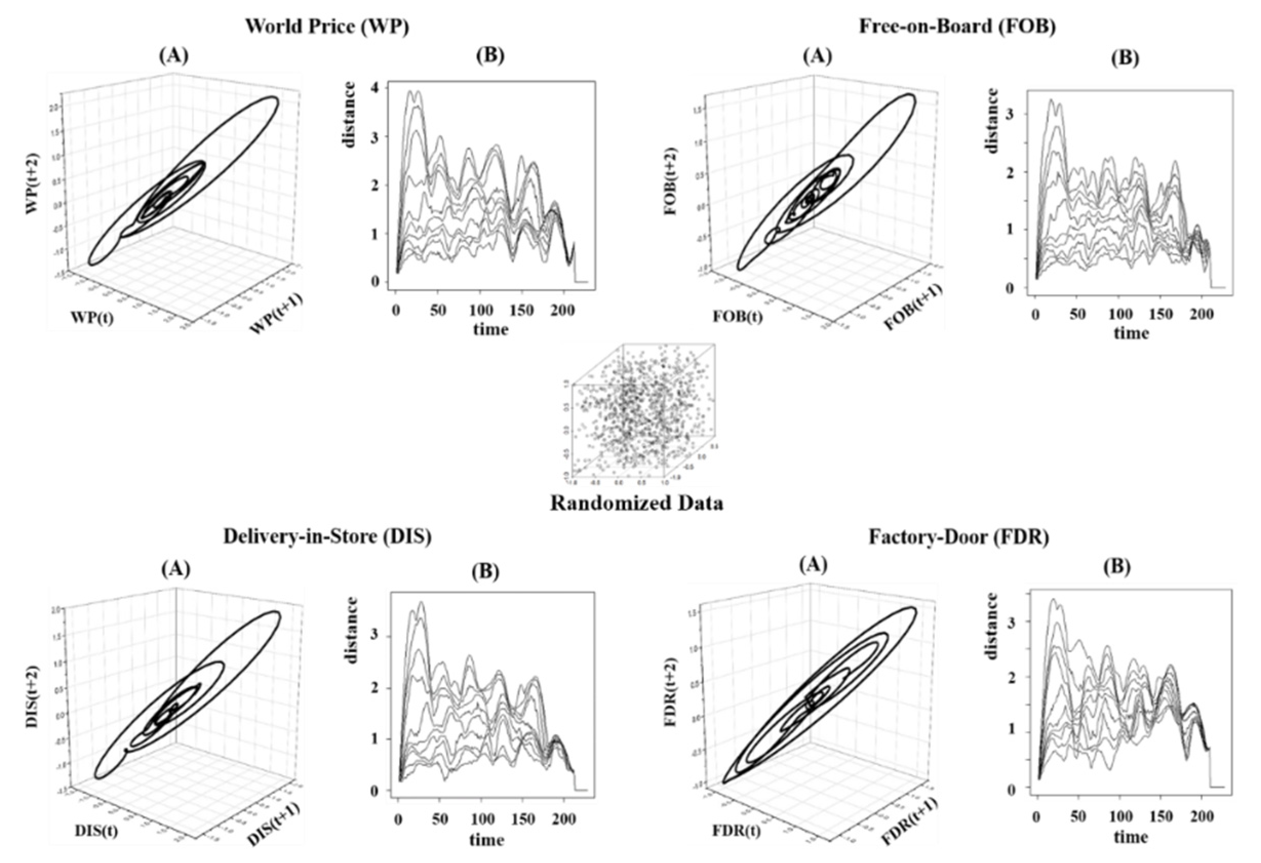
3.2. Stage 2: Reconstruct Market Dynamics from Price Signals

We next test whether the substantial structure isolated in each price series with SSA results from stable linearly stochastic or endogenously unstable nonlinear-deterministic real-world market dynamics. We first reconstruct state-space market attractors from each (detrended and denoised) price signal. Reconstructed attractors display geometric regularity whose outer orbits are due to lower-frequency cycles isolated by SSA, and inner orbits to higher-frequency cycles (Figure 6A). The regularity in these attractors, for example, is in stark contrast to the scattering of points reconstructed from a randomized (uniform) time series (middle inset plot). We use reconstructed attractors to test for stationarity of corresponding price signals with space-time separation plots (Figure 6B). The plots indicate stationarity of each price signal since initial cycles are completed with an elapsed time of about 50 months, which is sufficiently short relative to the 228-month period-of-record for successful operation of empirical nonlinear dynamic methods.

3.3. Stage 3: Test for Market Dynamics with Surrogate Price Data

Surrogate testing strongly rejects the null hypothesis that observed geometric regularity in market attractors reconstructed from coffee price signals along the global–domestic supply chain is incidentally due to linear-stochastic stable market dynamics (

Table 2. Stage 3: Test H₀—linear-stochastic dynamics ^a.

World Price	Signal b	Surrogate (low) c	H0 d
Permutation entropy	0.523	0.956	Reject
Free-on-Board
Permutation entropy	0.631	0.957	Reject
Delivery-in-Store
Permutation entropy	0.578	0.957	Reject
Factory Door
Permutation entropy	0.518	0.957	Reject

^a Randomized PPS [33] surrogate price vectors are generated to test the null hypothesis that apparent geometric regularity visualized in empirically reconstructed market attractors is generated by linear-stochastic dynamics. The significance level is set at α = 95% with 399 surrogates generated. The discriminating statistic is permutation entropy. ^b Discriminating statistics are taken from the market attractor reconstructed from each price series. ^c A lower-tailed test rejects the null hypothesis (H₀) if permutation entropy computed from the price-signal attractor rests below the ceiling of the lower extreme values computed from surrogate attractors. ^d Rejection of H₀ indicates that untested dynamic structures (such as nonlinear-deterministic dynamics) remain viable possibilities.

). Permutation entropies computed from price-signal attractors are substantially below the ceiling of the lower extreme values computed from surrogate attractors. Rejection of the null hypothesis indicates that untested dynamic structures (such as nonlinear-deterministic dynamics) remain viable possibilities. In sum, we have diagnosed that market dynamics along the global-PNG coffee supply chain are most likely structurally unstable. Spatial arbitrage does not stabilize prices; instead, persistently volatile prices oscillate irregularly along nonlinear market attractors.

Gelb (1979) also detected structurally unstable dynamics in an early study of US coffee prices, remarking that: “observers of the world coffee economy have sometimes also noted the existence of fairly slow but somewhat regular coffee price oscillations generally associated with severe structural disequilibria.” Past work attributed persistent structural disequilibria to the somewhat regular “coffee cycle” in which myopic producer investment response to current price levels leads to recurrent wide swings in coffee production and prices [41,43,44], and to failed industry and national stabilization policies [44]. Gelb (1979) questioned how endogenous cyclical oscillations persist when rational agents could realize above-normal profits by employing countercyclical investment strategies that would smooth out price cycles. He attributed persistence to: (1) “the impracticability of buffering the sequence of structural disequilibria in the product market because of the cost of holding the vast volume of required stocks”; (2) “the technological limitations on short-term output adjustment”; (3) “the inability of producers to predict coffee cycles to the extent required to formulate countercyclical strategies given the “stochastic nature (variable period) of the cycle.”

Our analysis of coffee prices after the turn of the 21st century offers compelling empirical evidence that—despite varietal, horticultural, infrastructural, and communicational advances—the above historic forces remain sufficiently strong that modern coffee markets continue to exhibit structural instability that, while having a stochastic appearance, is governed by nonlinear-deterministic dynamics.

Given that coffee prices in our study have a “deterministic” rather than a “stochastic” nature, why can producers not predict coffee cycles well enough to formulate countercyclical investment strategies? A surprising result of nonlinear dynamics is deterministic unpredictability: Long-term prediction in nonlinear dynamic systems is impossible even when governing laws are known with certainty due to sensitivity to initial conditions [16]. Trajectories emanating from two initially (very) close points on a nonlinear attractor diverge exponentially over time due to stretching and folding of the attractor. Given numerical imprecision of measuring initial conditions, computed trajectories along a nonlinear attractor will eventually evolve toward far different states. Although this limits the time horizon over which reliable predictions can be made, skillful short-term prediction is often possible.

3.4. Stage 4: Test for Price Transmission

Since we reject the null hypothesis of linear-stochastic stable market dynamics along the global-PNG coffee supply chain, we apply the CCM method to detect nonlinear price transmission in both upstream and downstream directions. CCM detects price transmission when the attractor reconstructed from the price receiving the transmission $\left(M_{RT}\right)$ can be used to skillfully predict values on the attractor reconstructed from the transmitting price $\left(M_T\right)$. The CCM plot for each pairwise price interaction is shown in Figure 7. Vertical axes measure predictive skill given by the Pearson correlation coefficient (ρ) between actual and predicted points on $M_T$. More skillful prediction is indicated as correlation coefficients converge to higher values (upper limit of one) as the library of price observations used to reconstruct $M_{RT}$ increases (horizontal axis). Statistically significant cross-mappings must rest above upper 95% confidence bounds on the predictive skill of predicting point on $M_T$ with attractors reconstructed from randomized surrogate prices (red curves). Above each CCM plot, we denote successful cross-mappings indicating price transmission by a solid black arrow, and unsuccessful cross-mappings indicating no price transmission by an outlined arrow with a line through it. Rightward (leftward) arrows indicate upstream (downstream) price transmission from WP→FOB→DIS→FDR (WP←FOB←DIS←FDR).

In Figure 7A, CCM detects upstream price transmission from world prices (WP) to both exporter (FOB) and factory (DIS) prices, from exporter to factory prices, but no statistically significant downstream transmission to producer prices (FDR). In Figure 7B, CCM detects that both producer (DIS) and factory (FDR) prices are transmitted downstream to exporter prices (FOB) as factors determining the differential that exporters calculate to tie their prices to world prices. CCM detects no downstream price transmission from the domestic market to world prices as expected since the PNG coffee exports a small fraction of global supply.

In Figure 8A, these detected pairwise price transmissions are summarized in a price transmission diagram in which circular nodes depict price signals and incoming (outgoing) arrows denote received (sent) price transmissions. The diagram clearly depicts how producers are isolated along the global-PNG coffee supply chain since no upstream price transmissions reach them.

Market power along the supply chain is often identified as a major driver of incomplete price transmission, but there may be other forces at work [45]. Bettendorf and Verboven (2000) found that weak transmission of coffee bean prices to consumer prices in the relatively competitive coffee market in the Netherlands was due to the relatively large share of non-bean costs in a relatively competitive coffee market [46]. This might explain the failure of upstream price transmission to PNG producers given that: (1) exporters set price differentials paid to upstream processors and producers covering both bean and non-bean costs; (2) the PNG coffee market is relatively competitive with large numbers of exporters and processors competing for limited PNG coffee production [23].

3.5. Quantification of Price Transmission

In Figure 8B, we construct a market attractor for the PNG coffee market composed of the mutually transmissive price signals along the supply chain: WP, FOB, and DIS. The S-mapping method [38] uses this attractor to quantify the economic impact of detected price transmissions along the supply chain as partial derivatives measuring the marginal change in the price receiving the transmission given an incremental change in the transmitting price over each month in the period-of-record (Figure 9).

The marginal response of exporter prices to an incremental increase in global prices (∂FOB/∂WP) was overwhelmingly negative through time (Figure 9A). The roots of this perhaps unexpected inverse relationship appear linked with how differentials (black curve) behaved over time in response to a low-frequency (57 month) cycle in world prices (gray curve) isolated with SSA (Figure 9B). Differentials were generally below average (standardized values negative) when world prices along the 57-month cycle were increasing, and above average when world prices along the 57-month cycle were decreasing. This is especially obvious after the 2011 peak in world prices. Additionally, it is of interest that the magnitude and frequency of above-average differentials after 2011 accompanied the increasing trend in the fraction of higher-grade (A and X) coffees produced in the PNG market (red curve). Prices paid by exporters to factories (DIS) also displayed a strong inverse marginal response to WP (Figure 9C).

Exporters and factories bilaterally transmitted price information (Figure 9D). The increasing fraction of higher grades A and X means increasing supply from estates and block holders, and therefore an increasing share of vertically integrated firms who are producers, processors, and exporters. Therefore, bicausal information flows. The downstream marginal impact on factory prices of an incremental increase in exporter prices (∂DIS/∂FOB) was largely negative over time (red area). Alternatively, the upstream marginal impact of factory prices on exporter prices (∂FOB/∂DIS, black area) resonated with the 57-month cycle in WP (gray curve). When WP cycled above average (standardized values positive), ∂FOB/∂DIS and ∂DIS/∂FOB were generally both negative. In an ecosystem analogy, the mutually detrimental prices were competitive. When WP cycled below average (standardized values negative), ∂FOB/∂DIS was generally positive. Paired with negative ∂DIS/∂FOB, we see that exporter prices marginally benefitted from incremental increases in factory prices while factory prices marginally declined in response to incremental increases in exporter prices. Continuing the ecosystem analogy, the relationship between exporter and factory prices switched from competitive to predator (exporter)-prey (factory).

Exporter prices marginally increased in response to an incremental increase in producer prices (∂FOB/∂FDR > 0) in two thirds of the months in the period-of-record, and marginally decreased in the remaining third (Figure 9E).

3.6. Implications for PNG Global–Domestic Supply Chain

Our results offer empirical evidence of upstream price transmission from the global market to domestic exporters and processors, but not through to coffee producers. The implications of these results for the PNG global–domestic supply chain depend on the factors causing weak price transmission. Past work emphasizes that price-transmission detection stops short of identifying causal factors [1,47], and consequently must be complemented with “qualitative information on the major factors that may determine the extent of transmission” [1]. Proposed causal factors have included “the degree of market power exerted by agents in the supply chain” [1], and raw commodity values that are only a small portion of final retail value [48]. Ghosray and Mohan (2021) detected asymmetric price adjustment between retail and international coffee prices that they attributed to “market concentration in the coffee supply chain at the coffee-roasting level, which allows coffee roaster to keep a higher share of the profits” [9]. Alternatively, Bettendorf and Verboven (2000) detected weak price transmission between coffee beans and final consumer price that they explained by “relatively large share of costs other than bean costs” [46]. Our description of the PNG coffee industry above (Section 2.1) does not support market concentration as a causal factor of weak (statistically insignificant) upstream price transmission to domestic producers since “[i] ntense competition among a large number of exporters and processors for limited PNG coffee production often leads to price wars.” Rather, the wide margin between exporter/processing prices (WP/DIS) and producer prices (FDR) over time (Figure 1) offers a more compelling driving factor in line with Bettendorf and Verboven (2000). This indicates that weak transmission to producers is not a market failure but a reflection of the substantial processing required to transform raw production to an exportable good. Consequently, public policy should protect producer (rural) incomes with extra-market tools (such as price supports) rather than market interference.

4. Conclusions

In this paper, we followed an inductive science approach to infer causal structure from observational data. We provided positive analysis of behavior that “actually happened” supplemented with qualitative explanations drawn from past studies. Our diagnostics were data-driven and not biased by imposing self-correcting markets whose failure to hold in the real world would result in selection of inappropriate price-transmission detection methods. Our results provide an empirical benchmark corresponding to real-world coffee market dynamics that can guide subsequent theory-based modeling. This benchmark includes a geometric picture of real-world state-space dynamics along the market supply chain that model output should reproduce, and detection and quantification of price transmission.

We emphasize that neither conventional price-stabilizing linear-stochastic market dynamics or endogenously unstable nonlinear-deterministic market dynamics should be presumptively ruled out as a plausible explanation for observed price volatility. We recommend that price transmission studies take advantage of recent developments in nonlinear dynamics to initially test for which explanation best corresponds to real-world markets before “straightjacketing” the analysis with either.

We conclude with a broad caveat: We cannot reasonably expect to successfully reconstruct deterministic nonlinear dynamics from observational data in every application. The dynamics of a real-world system might not evolve along a low-dimensional nonlinear attractor, or available data may not adequately sample an existing real-world attractor. We can reasonably expect to reconstruct a “sampling” of a real-world attractor [49] if available data adequately represent the dominant time scales of the system, or are not too noisy to detect deterministic behavior [49].

References

1. Rapsomanikis, G.; Hallam, D.; Conforti, P. Market Integration and Price Transmission in Selected Food and Cash Crop Markets of Developing Countries: Review and Applications. Available online: www.fao.org/3/YR117E/y5117e06.htm (accessed on 8 December 2020).
2. Brundtland Commission. Our Common Future; World Commission on Environment and Development: Oxford, UK, 1987. [Google Scholar]
3. Arrow, K.; Dasgupta, P.; Goulder, L.; Daily, G.; Ehrlich, P.; Heal, G.; Levin, S.; Maler, K.; Starrett, D.; Walker, B. Are we consuming too much. J. off Econ. Perspect. 2004, 18, 147–172. [Google Scholar] [CrossRef] [Green Version]
4. Fackler, P.; Goodwin, B. Spatial price analysis. In Handbook of Agricultural Economics; Gardner, B., Rausser, G., Eds.; Elsevier Science: Amsterdam, The Netherlands, 2002. [Google Scholar]
5. Engle, R.; Granger, C. Cointegration and error correction: Respresentation, estimation and testing. Econometrica 1998, 55, 40–47. [Google Scholar]
6. Sexton, R.; Kling, C.; Carman, H. Market integration, efficiency of arbitrage and imperfect competition: Methodology and application to US celery. Amer. J. Agr. Econ. 1991, 73, 568–580. [Google Scholar] [CrossRef] [Green Version]
7. Goodwin, B.; Piggot, N. Spatial market integration in the presence of threshold effects. Amer. J. Agr. Econ. 2001, 83, 302–317. [Google Scholar] [CrossRef] [Green Version]
8. Balcombe, K.; Rapsomanikis, G. Baysian estimation and selection of nonlinear vector error correction models: The case of the sugar-ethanol-oil nexus in Brazil. Amer. J. Agric. Econ. 2008, 90, 658–668. [Google Scholar] [CrossRef]
9. Ghosray, A.; Mohan, S. Coffee price dynamics: An analysis of the retail-international price margin. Eur. Rev. Agric. Econ. 2021, 1–24. [Google Scholar] [CrossRef]
10. Glendinning, P. Stability, Instability and Chaos: An Introduction to the Theory of Nonlinear Differential Equations; Cambridge University Press: Cambridge, UK, 1994. [Google Scholar]
11. Chavas, J.; Holt, M. On nonlinear dynamics: The case of the pork cycle. Am. J. Agric. Econ. 1991, 73, 819–828. [Google Scholar] [CrossRef]
12. Chavas, J.; Holt, M. Market instability and nonlinear dynamics. Am. J. Agric. Econ. 1993, 75, 113–120. [Google Scholar] [CrossRef]
13. Jensen, R.; Urban, R. Chaotic price behavior in a non-linear cobweb model. Econ. Lett. 1984, 15, 235–240. [Google Scholar] [CrossRef]
14. Berg, E.; Huffaker, R. Economic dynamics of the German hog-price cycle. Int. J. Food Syst. Dyn. 2015, 6, 64–80. [Google Scholar]
15. If economists reformed themselves. The Economist, 16 May 2016.
16. Kantz, H.; Schreiber, T. Nonlinear Time Series Anaysis; Cambridge University Press: Cambridge, UK, 1997. [Google Scholar]
17. Huffaker, R.; Bittelli, M.; Rosa, R. Nonlinear Time Series Analysis with R; Oxford University Press: Oxford, UK, 2017. [Google Scholar]
18. Huffaker, R.; Canavari, M.; Munoz-Carpena, R. Distinguishing between endogenous and exogenous price volatility in food security assessment: An empirical nonlinear dynamics approach. Agric. Syst. 2018, 160, 98–109. [Google Scholar] [CrossRef]
19. Huffaker, R.; Fearne, A. Reconstructing systematic persistent impacts of promotional marketing with empirical nonlinear dynamics. PLoS ONE 2019, 14, e0221167. [Google Scholar] [CrossRef]
20. Huffaker, R.; Hartmann, M. Reconstructing dynamics of foodborne disease outbreaks in the US cattle market from monitoring data. PLoS ONE 2021, 16, e0245867. [Google Scholar] [CrossRef] [PubMed]
21. McCullough, M.; Huffaker, R.; Marsh, T. Endogenously determined cycles: Empirical evidence from livestock industries. Nonlinear Dyn. Psychol. Life Sci. 2012, 16, 205–231. [Google Scholar]
22. Oreskes, N.; Shrader-Frechette, K.; Belitz, K. Verification, validation, and confirmation of numerical models in the earth sciences. Science 1994, 263, 641–646. [Google Scholar] [CrossRef] [PubMed] [Green Version]
23. Dambui, C.; Griffith, G.; Mounter, S. Short run coffee processor and expoerter marketing margin behavior in Papua New Guinea. In Proceedings of the International European Forum on System Dynamics and Innovation in Food Networks, Igls, Australia, 15 February 2015. [Google Scholar]
24. C.I.C. I.C. Statistical Database; G. CIC Ltd.: Toronto, ON, Canada, 1999–2017. [Google Scholar]
25. Papua New Guinea. Available online: https://www.bankpng.gov.pg/historical-exchange-rates/ (accessed on 11 August 2021).
26. Golyandina, N.; Nekrutkin, V.; Zhigljavsky, A. Analysis of Time Series Structure; Chapman & Hall/CRC: New York, NY, USA, 2001. [Google Scholar]
27. Schreiber, T. Detecting and analyzing nonstationarity in a time series with nonlinear cross predictions. Phys. Rev. Lett. 1997, 78, 843–846. [Google Scholar] [CrossRef] [Green Version]
28. Sprott, J. Chaos and Time Series Analysis; Oxford University Press: Oxford, UK, 2003. [Google Scholar]
29. Takens, F. Detecting strange attractors in turbulence. In Dynamical Systems and Turbulence; Rand, D., Young, L., Eds.; Springer: New York, NY, USA, 1980; pp. 366–381. [Google Scholar]
30. Deyle, E.; Sugihara, G. Generalized theorems for nonlinear state space reconstruction. PLoS ONE 2011, 6, 1–8. [Google Scholar] [CrossRef]
31. Provenzale, A.; Smith, L.; Vio, R.; Murante, G. Distinguishing between low-dimensional dynamics and randomness in measured time series. Phys. D 1992, 58, 31. [Google Scholar] [CrossRef]
32. Theiler, J.; Eubank, S.; Longtin, A.; Galdrikian, B.; Farmer, J. Testing for nonlinearity in time series: The method of surrogate data. Phys. D 1992, 58, 77–94. [Google Scholar] [CrossRef] [Green Version]
33. Small, M.; Tse, C. Applying the method of surrogate data to cyclic time series. Phys. D 2002, 164, 187–201. [Google Scholar] [CrossRef]
34. Brandt, C.; Pompe, B. Permutation entropy: A natural complexity measure for time series. Phys. Rev. Lett. 2012, 88, 174102. [Google Scholar] [CrossRef]
35. Schreiber, T.; Schmitz, A. Surrogate time series. Phys. D 2000, 142, 346–382. [Google Scholar] [CrossRef] [Green Version]
36. Sugihara, G.; May, R.; Hao, Y.; Chih-hao, H.; Deyle, E.; Fogarty, M.; Munch, S. Detecting causality in complex ecosystems. Science 2012, 338, 496–500. [Google Scholar] [CrossRef]
37. Muir, J. My First Summer in the Sierra; Houghton Mifflin: Boston, MA, USA, 1911. [Google Scholar]
38. Deyle, E.; May, R.; Munch, S.; Sugihara, G. Tracking and forecasting ecosystem interactions in real time. Proc. R. Soc. B 2018, 283, 201522358. [Google Scholar] [CrossRef]
39. Version, Origin. Version 2019. Available online: https://www.originlab.com/ (accessed on 10 August 2021).
40. Gelb, A. A spectral analysis of coffee market oscillations. Int. Econ. Rev. 1979, 20, 495–514. [Google Scholar] [CrossRef]
41. Jacob, H. The Saga of Coffee: The Biography of an Economic Product; Allen and Unwin: London, UK, 1935. [Google Scholar]
42. Terazono, E. Brazilians smooth out arabica output cycle. Financial Times, 30 January 2013. [Google Scholar]
43. Delfim-Netto, A.; Pinto, C. Brazilian coffee: 20 years of substitution in the international market. ANPES Study 1965, 3. [Google Scholar]
44. Geer, T. An Oligopoly: The World Coffee Economy and Stabililization Schemes; Dunellen: New York, NY, USA, 1974. [Google Scholar]
45. Vavra, P.; Goodwin, B. Analysis of price transmission along the food chain. In OECD Food, Agriculrual and Fisheries Working Papers; OECD Publishing: Paris, France, 2005. [Google Scholar]
46. Bettendorf, L.; Verboven, F. Incomplete transmission of cofee bean prices in the Netherlands. Eur. Rev. Agric. Econ. 2000, 27, 1–16. [Google Scholar] [CrossRef]
47. OECD Competition Committee. Competition Issues in the Food Chain Industry; Competition Law & Policy OECD: Paris, France, 2013. [Google Scholar]
48. Kim, H.; Ward, R. Price transmission across the U.S. food distribution system. Food Policy 2013, 41, 226–236. [Google Scholar] [CrossRef]
49. Ghil, M.; Allen, M.; Dettinger, M.; Ide, K.; Kondrashov, D.; Mann, M.; Robertson, A.; Saunders, A.; Tian, Y.; Varadi, F.; et al. Advanced spectral methods for climatic time series. Rev. Geophys. 2002, 40, 1–41. [Google Scholar] [CrossRef] [Green Version]
Figure 1. World and domestic coffee prices. (A) The monthly price series extend from January 1999 to December 2017 (period-of-record is 228 months). The world price (WP) is the New York futures price. Domestic coffee prices in the Papua New Guinea (PNG) market include: (1) the Free-on-Board price (FOB)—the export price—which adds a premium or deducts a discount from WP (called the differential) determined by the quality grade of coffee (A and X are premium grades) and market conditions; (2) the delivery-in-store price (DIS) paid by exporters to processors; (3) the factory door price (FDR) paid to growers. (B) As WP trended upward toward the 2011 peak (black curve), the differential between FOB and WP (blue area) was negative. However, after 2011, the differential switched to positive during months of sustained WP decrease (red segments). This is suggestive of price leveling behavior by exporters.
Sustainability 13 09172 g001
Figure 2. A framework for empirically detecting and quantifying price transmission. Stage 1 initially prepares price time-series data for empirical nonlinear dynamic methods with signal processing to remove noise and test for nonlinear stationarity. Stage 2 reconstructs market dynamics from denoised stationary price data, and Stage 3 statistically tests whether reconstructed dynamics are most likely driven by stable linear-stochastic or endogenously unstable nonlinear-deterministic market dynamics. In Stage 4, test results guide us to causal detection and quantification methods corresponding best to reconstructed real-world market dynamics.
Sustainability 13 09172 g002
Figure 3. Delayed-coordinate embedding. We illustrate the use of delayed-coordinate embedding to reconstruct state-space dynamics from a single time series: x(t) = (1, 2, 3, 1, 2). First, an embedded data matrix is constructed whose first column is the observed time series and remaining columns are lagged copies. The figure shows the 3 × 3 embedded data matrix for x(t) with a time delay of a single period (embedding delay) and three lagged copies which serve as the coordinate axes of reconstructed phase space (embedding dimension).
Sustainability 13 09172 g003
Figure 4. Stage 1: Signal processing to detrend prices. (A) Low-frequency nonlinear trend cycles (blue cycles) are removed because they cannot be adequately sampled from the observed price series (black curves). The world price (WP) series (gray curve) and isolated nonlinear trend cycle (dashed blue curve) are extended two years beyond the period-of-record of the domestic prices to demonstrate that the trend cycle has a length of about 18 years (2002–2020), a trend-cycle length also detected in an early spectral analysis of historic US coffee prices [40]. (B) To explain the market underpinnings of trended behavior, the trends are annualized (by taking the annual average of monthly prices) so that they can be compared with annual production and inventory data provided by the ICO. At peak WP in 2011, the coffee inventory of the largest importing nations was at a 10-year minimum (red curve). Inventory subsequently increased rapidly in response to upward trending production (blue curve) resulting in a sustained decline in trended prices through the end of the period-of-record.
Sustainability 13 09172 g004
Figure 5. Signal processing of detrended prices. Higher-frequency cyclical components are isolated in the (detrended) residuals from the initial application of SSA. The columns of the figure show signal processing for each detrended price series. The top row of the figure plots isolated signals (black curve) against the detrended time series (gray curves). Signals tract the corresponding detrended price series closely, indicating that structured variation accounts for a high percentage of total variation in each detrended series. The middle row of the figure plots the oscillatory components of structured variation for each price signal. The bottom row of the figure shows the unstructured variation (noise) isolated in each detrended price series (red curves).
Sustainability 13 09172 g005
Figure 6. Stage 2: Reconstruct state-space dynamics from detrended price signals. (A) Reconstructed state-space market attractors from each detrended price signal exhibit a geometric regularity that, for example, is in stark contrast to the random scattering of points reconstructed from a randomized (uniform) time series (middle inset plot). (B) Space-time separation plots indicate that each price signal is stationarity since initial cycles (completed with an elapsed time of about 50 months) are short relative to the 228-month period-of-record.
Sustainability 13 09172 g006
Figure 7. Stage 4: Test for price transmission with convergent cross mapping (CCM). The CCM algorithm of Sugihara et al. (2012) [36] detects price transmission when the attractor reconstructed from the price receiving the transmission ( M R T ) skillfully predict values on the attractor reconstructed from the transmitting price ( M T ) . Vertical axes of CCM plots measure predictive skill given by the Pearson correlation coefficient (ρ) between actual and predicted points on M T , and horizontal axes measure the library of price observations used to reconstruct M R T . More skillful prediction is indicated as correlation coefficients converge to higher values (upper limit of one) as the library increases. Statistically significant cross-mappings must rest above upper 95% confidence bounds on the predictive skill of predicting point on M T (red curves). Price transmission is denoted by a solid black arrow, and no price transmission by an outlined arrow with a line through it. Rightward (leftward) arrows indicate upstream (downstream) price transmission from WP→FOB→DIS→FDR (WP←FOB←DIS←FDR). (A) Upstream price transmission. CCM detects upstream price transmission from world prices (WP) to both exporter (FOB) and factory (DIS) prices, from exporter to factory prices, but no statistically significant upstream transmission to producer prices (FDR). (B) Downstream price transmission. CCM detects no downstream price transmission from the domestic market to world prices as expected since the PNG coffee exports a relatively small fraction of global supply. Both producer (DIS) and factory (FDR) prices are transmitted downstream to exporter prices (FOB) as factors determining the differential that exporters calculate to tie their prices to world prices.
Sustainability 13 09172 g007
Figure 8. Price transmission in world-PNG coffee market. (A) In a price transmission diagram, circular nodes depict price signals and incoming (outgoing) arrows denote received (sent) transmissions. Producers are largely isolated along the global-PNG coffee supply chain since no upstream price transmissions reach them. (B) A market attractor for the PNG coffee market—composed of the interactive top (upstream) links of the supply chain (WP, FOB, and DIS)—is used to quantify the economic impact of detected price transmissions with S-mapping [38].
Sustainability 13 09172 g008
Figure 9. Stage 4: Quantify the economic impact of price transmission. The S-mapping method uses the PNG coffee market attractor constructed from the most interactive price signals along the supply chain (Figure 8B) to compute partial derivatives measuring the marginal change in the price receiving the transmission given an incremental change in the transmitting price over the period-of-record. (A) The marginal response of exporter prices to an incremental increase in global prices (∂FOB/∂WP) was overwhelmingly negative through time. (B) The rationale for this inverse relationship is illuminated by observing that differentials (black curve) were generally below average (standardized values negative) when world prices along the 57-month cycle (gray curve) were increasing, and above average when world prices along the 57-month cycle were decreasing. (C) Prices paid by exporters to factories (DIS) also displayed a strong inverse marginal response to WP. (D) Exporters and factories had bilateral price transmission. When WP cycled above average (standardized values positive), ∂FOB/∂DIS and ∂DIS/∂FOB were generally both negative suggesting a mutually detrimental competitive interaction. When WP cycled below average (standardized values negative), ∂FOB/∂DIS turned positive suggesting that the relationship between exporter and factory prices switched from competitive to predator (exporter)-prey (factory). (E) Exporter prices marginally increased in response to an incremental increase in producer prices (∂FOB/∂FDR > 0) in two thirds of the months in the period-of-record, and marginally decreased in the remaining third.
Sustainability 13 09172 g009