
Does ESG Impact Really Enhance Portfolio Profitability?


Department of Business Studies, Roma Tre University, 00145 Rome, Italy
*
Author to whom correspondence should be addressed.
Sustainability 2022, 14(4), 2050; https://doi.org/10.3390/su14042050
Submission received: 28 December 2021
/
Revised: 26 January 2022
/
Accepted: 2 February 2022
/
Published: 11 February 2022
(This article belongs to the Special Issue Sustainable Portfolio Management)
Abstract
:Over the last few decades, growing attention to the topic of social responsibility has affected financial markets and institutional authorities. Indeed, recent environmental, social, and financial crises have inevitably led regulators and investors to take into account the sustainable investing issue; however, the question of how Environmental, Social, and Governance (ESG) criteria impact financial portfolio performances is still open. In this work, we examine a multi-objective optimization model for portfolio selection, where we add to the classical Mean-Variance analysis a third non-financial goal represented by the ESG scores. The resulting optimization problem, formulated as a convex quadratic programming, consists of minimizing the portfolio variance with parametric lower bounds on the levels of the portfolio expected return and ESG. We provide here an extensive empirical analysis on five datasets involving real-world capital market indexes from major stock markets. Our empirical findings typically reveal the presence of two behavioral patterns for the 16 Mean-Variance-ESG portfolios analyzed. Indeed, over the last fifteen years we can distinguish two non-overlapping time windows on which the inclusion of portfolio ESG targets leads to different regimes in terms of portfolio profitability. Furthermore, on the most recent time window, we observe that, for the US markets, imposing a high ESG target tends to select portfolios that show better financial performances than other strategies, whereas for the European markets the ESG constraint does not seem to improve the portfolio profitability.
1. Introduction
Socially Responsible Investment (SRI), also called “ethical investment” or “sustainable investment”, is typically defined as a decision-making approach that integrates environmental, social, and ethical features into the investment process (Sandberg et al. [1] and Martini [2]).
Over the past decades, the popularity and significance of SRI have considerably and rapidly grown (see, e.g., Sparkes and Cowton [3]). As reported by the Global Sustainable Investment Alliance (GSIA) in the yearly Global Sustainable Investment Review [4], “sustainable investment is a major force shaping global capital markets, and, in turn, is influencing companies and others seeking to raise capital in those global markets”. Furthermore, sustainable investment in the leading world markets (e.g., United States, Canada, Japan, Australasia, and Europe) has reached USD 35.3 trillion in assets under management, having grown by 15% in two years.
The SRI development finds its origins in several historical events such as financial crises, natural disasters, increasing attention to the defense of human rights and changes in climatic conditions, which have led policy-makers and financial operators to address the socially responsible investing issue. Its three main pillars are Environmental, Social, and corporate Governance (ESG). These factors, suitably combined, can be used to build a score that is able to assess companies and investments in terms of sustainability. Indeed, as described by Widyawati [5] through a detailed literature review on SRI, ESG metrics can play a central role in empirical studies since they are used as a proxy of sustainability performance (see also Billio et al. [6], Chatterji et al. [7], Berg et al. [8], Li et al. [9], and Oliver [10]).
The aim of this study is to investigate the in-sample and out-of-sample effects of the ESG rating on the portfolio selection process and to analyze its impact in terms of portfolio profitability and risk, giving a look at the SRI regulatory framework developments over years. For this purpose, we consider a multi-objective portfolio optimization model, where we add to the classical Mean-Variance analysis a third non-financial goal represented by the ESG score. The resulting tri-objective optimization problem is formulated as a convex Quadratic Programming (QP), and consists of minimizing the portfolio variance with parametric lower bounds on the levels of the portfolio expected return and the portfolio ESG. We then provide an extensive empirical analysis over the period 2006–2020 using five real-world datasets from the major stock markets. To better examine the ESG impact on portfolio performance and to capture possible effects of SRI regulatory developments over the past 15 years, we conducted the out-of-sample performance analysis using both the full length of data available and two non-overlapping subperiods.
Our empirical findings typically reveal the presence of two behavioral patterns for the 16 Mean-Variance-ESG efficient portfolios analyzed. Over the last fifteen years we can distinguish two non-overlapping time windows on which the inclusion of portfolio ESG targets leads to different regimes in terms of portfolio profitability. Some similar evidence can be found in Bermejo et al. [11], where the authors show that the ESG disclosure is positively related to the portfolio excess return and contributes to its stability over time. They also observe a regime change around 2015, when the so-called Paris Agreement [12] was signed (for more details, see Section 2). On the most recent time window we observe that, for the US markets, imposing a high ESG target tends to select portfolios that show better financial performances than the other strategies. Furthermore, we can note that the sustainability-focused strategies continue to show positive effects on the financial markets even during the recent COVID-19 pandemic crisis. Indeed, as also highlighted by Nofsinger and Varma [13], the positive socially responsible actions of companies could make them more profitable even in times of crisis. On the other hand, in European markets, in particular, in the Euro Stoxx 50, the portfolio performances do not seem to be affected by imposing ESG constraints, as also pointed out by La Torre et al. [14]. Contributions similar to this study can be also found in the works of Amon et al. [15,16], where the authors examine the impact of the ESG-based investment strategies on the portfolio performance, analyzing and comparing European and US markets.
The rest of the paper is organized as follows. In Section 2, we give a brief review of the literature relevant to this study. Section 3 introduces the Mean-Variance-ESG model and shows the main properties of the corresponding Pareto-optimal portfolios in terms of gain, risk, and ESG tradeoff. Section 4 provides a detailed out-of-sample performance analysis on five real-world datasets. Finally, in Section 5 we draw some concluding remarks, highlighting the main contributions of our work to the literature.
2. Literature Overview
ESG was mentioned for the first time in “Who Cares Wins 2005 Conference Report” [17], where institutional investors and regulators emphasized the importance of ESG factors in asset management and in financial research. Since then, the ESG metrics evolved and many countries around the world started coordinating to promote the development of a common framework for sustainable finance (see [18]). Following that global trend, several scholars attempted to examine the impact of ESG factors on portfolio selection process for achieving better sustainability goals. For instance, Van Duuren et al. [19] studied how fund managers across several countries in the world deal with the ESG integration in the investment management process. Their findings show significant differences in terms of perception of SRI investment among US, UK, and European fund managers. Bermejo et al. [11] found a direct relation between the level of ESG disclosure and corporate performances, focusing on the European market; however, an extensive literature has fueled over years the debate on the relationship between ESG rating and financial performance, which is still open (see, e.g., Brunet [20], Derwall et al. [21], and Nofsinger and Varma [13]). Friede et al. [22] provided a comprehensive overview of more than 2000 empirical academic studies on ESG investing, showing that in almost 90% there is a positive and stable relationship over time between ESG and corporate financial performance. More recent works confirmed these findings (see, e.g., Brooks and Oikonomou [23], Starks et al. [24]), also highlighting that ESG features positively impact on the mitigation of tail risks (Giese and Lee [25]).
Since the ESG concept was formally proposed in the early 2000s, many countries and institutions have subsequently proposed actions to promote the development of the ESG factors. As highlighted by Martini [2], the above mentioned SRI market growth could be justified by two main reasons. On one hand, the global financial crisis of 2007–2008 has inevitably highlighted the central role of corporate social responsibility on financial markets and, therefore, on the world economy in general. On the other hand, the desired challenges on issues such as climate change, pollution, and the waste of natural resources, have led to a major attention to global sustainability topics and, in turn, to the need for their regulations at global level. A clear example is one of the most significant environmental treaties ever negotiated, the 1997 Kyoto Protocol of the United Nations Framework Convention on Climate Change (UNFCCC, [26]), which only came into force in February 2005. Its aim was to promote the reduction in greenhouse emissions by means of specific measures on mitigation and producing periodic reports. The Kyoto Protocol has been originally structured on a commitment period ranging from 2005 to 2012 and then revised with the Doha Amendment [27], that establishes a further commitment period from 2013 to 2020. In 2006 the United Nations started a process to develop the Principles for Responsible Investment (PRI), an investor’s network whose aim was to support sustainable investments through the ESG factors. More recently, for the 2015 UNFCCC held in Paris (COP21), 196 countries agreed to adopt a universal and legally binding global climate agreement, defining a joint action plan to limit further harmful climate change, the so-called Paris Agreement [12].
Since we aim to investigate the ESG impact on portfolio performance and to capture possible effects of SRI regulatory developments over the past 15 years, we conducted the out-of-sample performance analysis using both the full length of data available and two non-overlapping subperiods that approximately cover the two commitment periods in which the Kyoto Protocol was structured with the Doha Amendment.
3. The Mean-Variance-ESG Model
In this section we describe the multi-objective portfolio selection model that we use to examine the impact of the ESG score on the portfolio risk and profitability. The resulting optimization problem is formulated as a parametric convex QP.
Let us first introduce some notations and concepts. We consider an investment universe of n assets, whose linear returns are represented by the random variables , and ESG scores by . We assume that the random variables representing the linear returns and the ESG scores are defined on a discrete probability space , where , a -field and . In this work, we adopt a look-back approach, where the possible realizations of the discrete random variables are obtained from historical data. Furthermore, the investment decision is made assuming T equally likely historical scenarios, as it is common in portfolio optimization (see, e.g., Carleo et al. [28], and references therein). In the case of long-only portfolios, we identify with the vector a feasible portfolio satisfying the budget constraint, where is the fraction of capital invested in asset k. The portfolio linear return is therefore defined as . For each and , we denote by the realized price of asset k at time t, and for , we denote by the realized (linear) return of asset k for the period ending at t. Thus, we indicate by the portfolio return at time t.
We recall here the classical Mean-Variance portfolio optimization model [29,30], whose aims are to determine the vector of portfolio weights minimizing the portfolio variance , while the portfolio expected return is constrained to attain a specified target level , where denotes the expected return of asset k, and indicates the covariance between assets k and j; therefore, the classical Mean-Variance model reads
where the last two constraints represent the budget and the no-short sellings constraints, respectively. This is a convex quadratic programming problem that can be solved by a number of efficient algorithms, ensuring a controlled computational effort (see, e.g., Cesarone et al. [31]).
Our aim is to include to the Mean-Variance model the maximization of the portfolio expected ESG, that is defined as , where denotes the expected ESG score assigned to asset k (see Utz et al. [32]); therefore, for the Mean-Variance-ESG approach, a portfolio x is preferred to a portfolio y if and only if , and , with at least one strict inequality. It follows that the efficient surface of the Mean-Variance-ESG model can be obtained by finding the non-dominated portfolios, which are the Pareto-optimal solutions of the following tri-objective optimization problem
We apply the standard -constraint method (see Ehrgott [33]) to reformulate Problem (2) into a single-objective optimization problem, as follows
where and are the required target levels of the portfolio expected return and ESG indicator, respectively. Hence, the resulting optimization problem is still a convex QP, and consists in minimizing the portfolio variance with parametric lower bounds on the levels of the portfolio expected return and ESG.
The Mean-Variance-ESG Pareto-optimal portfolios can be obtained as solutions of Problem (3) by appropriately varying the target level of the portfolio expected return and the target level of the portfolio expected ESG , as described in the next section.
3.1. Properties of the M-V-ESG Portfolios
In this section we show how to practically find the efficient surface of the Mean-Variance-ESG model by solving Problem (3) following a procedure similar to Roman et al. [34] and Cesarone et al. [35]. As mentioned above, we minimize the portfolio variance imposing parametric constraints on the the target level of the portfolio expected return and the target level of the portfolio expected ESG . Then, from (3) we can obtain all the non-dominated portfolios by a suitable varying of and . For this purpose, we first set an appropriate interval for , where , with and with . Then, for a fixed level of , we determine the suitable interval for the target level of the portfolio expected ESG . Here, , where is the minimum variance portfolio with a fixed lower bound for the portfolio expected return, namely it is the optimal solution of the following problem
On the other side, , where is the portfolio that maximizes the ESG indicator with a lower bound for the portfolio expected return, namely
In Figure 1 we provide an example of Mean-Variance-ESG efficient portfolios, represented in the variance-ESG plane for several fixed levels of the portfolio expected return .
Note that by solving Problem (3) with and with , we obtain the Mean-Variance efficient frontier (see the bold black dashed line). More specifically, when and , we have the Global Minimum Variance (GMinV) portfolio (see the bold x in Figure 1), whereas for the efficient frontier degenerates into one point, namely the portfolio composed of the asset with highest expected return. On the other hand, if we solve Problem (3) with and with , we obtain the ESG-mean efficient frontier (see the red dashed line).
From Figure 1 it is interesting to observe that when the target portfolio return increases, the in-sample variance of the corresponding efficient portfolios increases, whereas their ESG values decrease. Indeed, when the required target return level is low, say , the set of feasible portfolios is large and therefore diversification is high. This allows for the selection of Pareto-optimal portfolios with high sustainability (but with gradually increasing risk), or portfolios with low risk (but with gradually decreasing ESG). As the level of increases the set of feasible solutions of Problem (3) becomes smaller, such as the interval and the range of the optimal portfolio risk values. This is also confirmed in Section 4.1.1 by means of Figure 5, showing that when requiring high levels of ESG or of portfolio return, the number of selected assets in the Pareto-optimal solutions tends to decrease.
In Figure 2 we provide another example of the Mean-Variance-ESG efficient portfolios, represented in the variance-expected return plane for several fixed levels of the portfolio expected ESG . Note that if we solve Problem (3) by varying with , we obtain the ESG-variance efficient frontier (see the red dashed line). More specifically, when and , we obtain the Global Minimum Variance (GMinV) portfolio (see the bold x in Figure 2), whereas for the highest level of portfolio sustainability , the efficient frontier collapses in a single portfolio, the one composed by the asset with the highest expected ESG. On the other hand, when solving Problem (3) for different values of with , we have the mean-ESG efficient frontier (see the bold black dashed line). As expected, for fixed levels of portfolio sustainability, when requiring higher levels of the portfolio expected return, the corresponding efficient portfolios are riskier.
An alternative reformulation of Problem (2) can be obtained by maximizing the portfolio expected return with parametric lower bounds on the levels of the portfolio sustainability and with parametric upper bounds on the levels of the portfolio risk, as follows:
In Figure 3 we provide a third example of the Mean-Variance-ESG efficient surface, represented in the expected return-ESG plane for several levels of the portfolio variance .
We can observe that, for a fixed level of , if we require higher levels of the portfolio expected ESG, we have efficient portfolios with lower expected return, while if we impose higher levels of the portfolio expected return, we obtain Pareto-optimal portfolios with lower sustainability. Note that if we solve Problem (6) by varying with , we obtain the Mean-Variance efficient frontier (see the bold black dashed line in Figure 3). When , we obtain the Global Minimum Variance (GMinV) portfolio (see the bold x in Figure 3). On the other hand, when solving Problem (6) for several values of with , we obtain the ESG-variance efficient frontier (see the red dashed line in Figure 3).
Summing up, these in-sample results highlight a trade-off relationship between portfolio profitability, risk, and sustainability. In the next section, we examine the out-of-sample effects of the ESG rating on the portfolio selection process, looking for possible links with the different actions proposed by many countries and institutions over the years to promote the development of SRI.
4. Empirical Analysis
We provide here a detailed empirical analysis performed on five real-world datasets. More precisely, in Section 4.1 we describe the tested datasets, the methodology adopted for the experimental setup, and the portfolio strategies that we analyze, including the performance measures used for the out-of-sample performance evaluation. Section 4.1.1 reports the computational results examining the composition and diversification of the 16 Mean-Variance-ESG efficient portfolios examined. In Section 4.2 we report and discuss the out-of-sample performance results.
All the procedures have been implemented in MATLAB R2019b and have been executed on a laptop with an Intel(R) Core(TM) i7-8565U CPU @ 1.80 GHz processor and 8 GB of RAM.
4.1. Description of the Datasets and Methodologies
In this section, we provide some details about the five real-world datasets that are summarized in Table 1 and are publicly available on the website https://host.uniroma3.it/docenti/cesarone/DataSets.htm (accessed on 10 February 2022). These datasets consist of daily prices, adjusted for dividends and stock splits, and of daily ESG scores obtained from Refinitiv [36].
We have included stocks with at least ten years of observations, omitting the year 2021, due to a partial lack of data on ESG scores. Furthermore, to better examine the ESG impact on portfolio performance and to capture possible effects of SRI regulatory developments over the past 15 years, we use two different experimental setups, named Setup Entire and Setup Split. For Setup Entire, we consider the entire length of data available (October 2006–December 2020) to perform out-of-sample performance analysis. For Setup Split, we divide the full length of the time series into two equal time windows, i.e., October 2006–December 2013 and January 2014–December 2020. We point out that these two time windows have been chosen to focus on the two commitment periods, in which the Kyoto Protocol was structured with the Doha Amendment, and therefore to highlight possible different regimes in terms of profitability–sustainability.
For the two different experimental setups, we present the out-of-sample analysis of 16 Pareto-optimal portfolios obtained from Problem (3) by appropriately varying the target levels of the portfolio expected return and of the portfolio expected ESG (see Section 3.1). Figure 4 shows, in the variance-ESG plane, an example of the 16 portfolio strategies, which are characterized by several investor goals, for the DowJones dataset. More precisely, we consider four different levels of target return with , and, for each level , four different target ESG levels with . We point out that, when , we obtain Mean-Variance optimal portfolios (see the bold black dashed line in Figure 1 and related remarks), whereas when , we select ESG-mean optimal portfolios (see the red dashed line in Figure 1 and related remarks).
For the out-of-sample performance analysis, we adopt a rolling time window scheme of evaluation, namely we allow for the possibility of rebalancing the portfolio composition during the holding period at fixed intervals. In this study, we set 2 years (500 observations) for the in-sample window and 1 month (20 observations) both for the rebalancing interval and the holding period.
The out-of-sample performance of the 16 Mean-Variance-ESG efficient portfolios described above is evaluated using several performance measures typically adopted in the literature (see, e.g., Cesarone and Colucci [37], Bruni et al. [38], and references therein): mean, volatility, Sharpe ratio [39,40], Max Drawdown (see, e.g., Chekhlov et al. [41]), Ulcer index [42], Turnover (see, e.g., Han [43]), and Rachev ratio with confidence level of [44]. We also compute the so-called Return On Investment (ROI), namely the time-by-time return generated by each portfolio strategy over a specified time horizon . More precisely, ROI is defined as follows
where is the amount of capital invested at the beginning of the time horizon, is the portfolio wealth, and T is the number of historical scenarios.
4.1.1. Composition of the Mean-Variance-ESG Efficient Portfolios
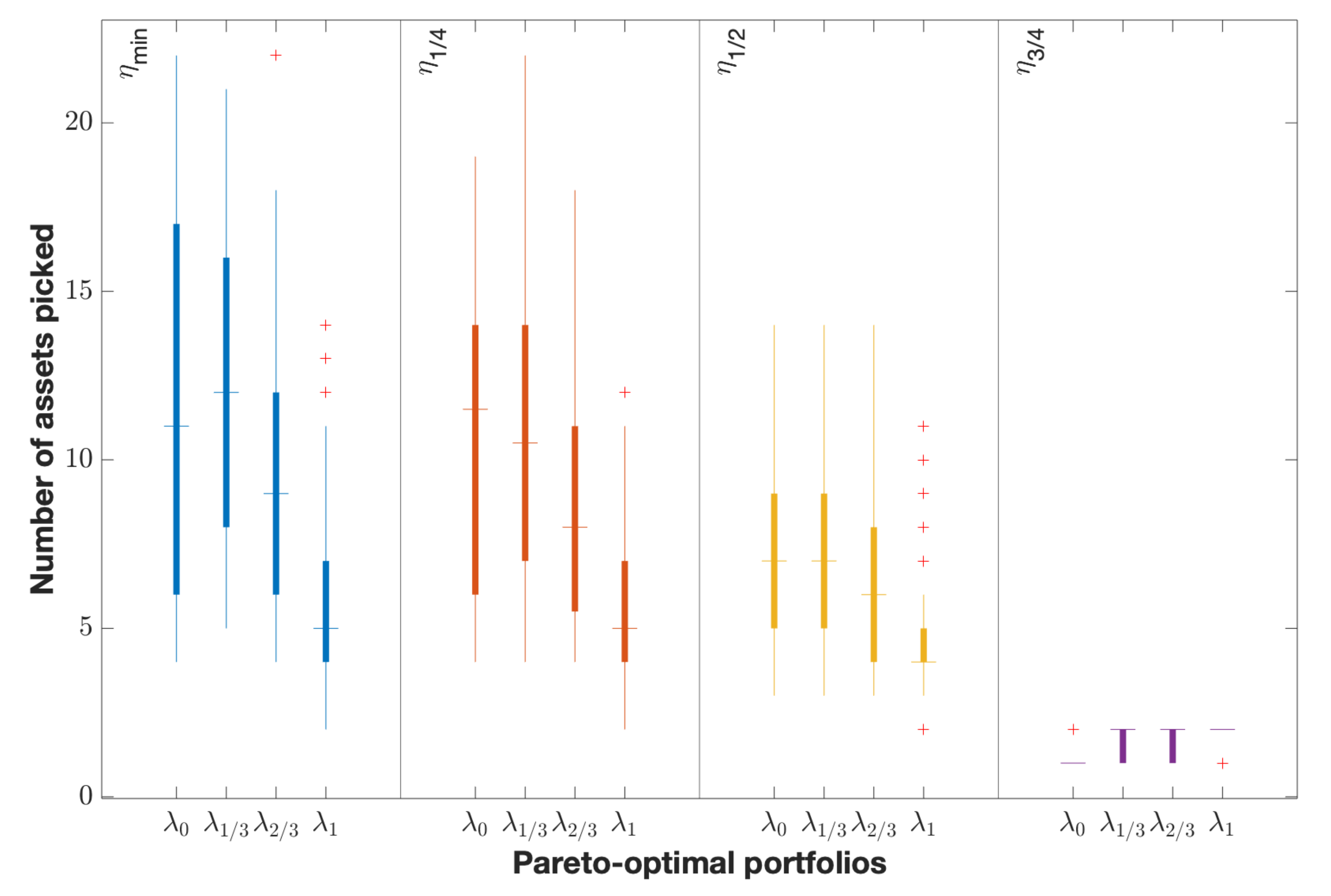
To obtain an insight of the composition and diversification of the 16 Pareto-optimal portfolios analyzed, in Figure 5 we show the box plots of the number of the selected assets for the DowJones dataset, adopting Setup Entire and the RTW scheme.
Then, each box provides the distribution of the number of the assets selected by the 16 portfolio strategies for all the in-sample windows tested. The central mark represents the median, and the bottom and top edges of the box are the 25th and the 75th percentiles, while the outliers are plotted individually. We observe that, for a fixed level of the portfolio target return , e.g., , when the portfolio sustainability increases the number of assets typically tends to decrease. Indeed, the Mean-Variance optimal portfolios, namely the Mean-Variance-ESG portfolios with , generally have more assets in their composition than the ESG-mean portfolios, namely those with .
4.2. Out-of-Sample Performance Analysis
In this section, we discuss the main results of the out-of-sample performance analysis for all the previously introduced 16 portfolio selection strategies. More precisely, in Section 4.2.1 and Section 4.2.2 we report the computational results obtained for the DowJones dataset with Setup Entire and Setup Split, respectively. Section 4.2.3 and Section 4.2.4 show the results obtained for the EuroStoxx50 dataset with Setup Entire and Setup Split, respectively. Finally, for the sake of completeness, in Appendix A we report the remaining out-of-sample performance results, obtained from the other datasets listed in Table 1.
In the tables of the following sections, for each investment universe we show with different colors the rank of the performance results of the proposed portfolio strategies. More in detail, for each row (performance measure) the colors span from deep-green to deep-red, where deep-green represents the best performance, while deep-red the worst one. This style of visualization could allow for easier detection of possible persistent behavioral patterns of a portfolio strategy (corresponding to a column).
4.2.1. Computational Results for DowJones with Setup Entire
Table 2 reports the out-of-sample performance evaluated by Mean, Volatility, Sharpe ratio, Max Drawdown (MaxDD), Ulcer index, Turnover, and Rachev 5% ratio (see Section 4.1).
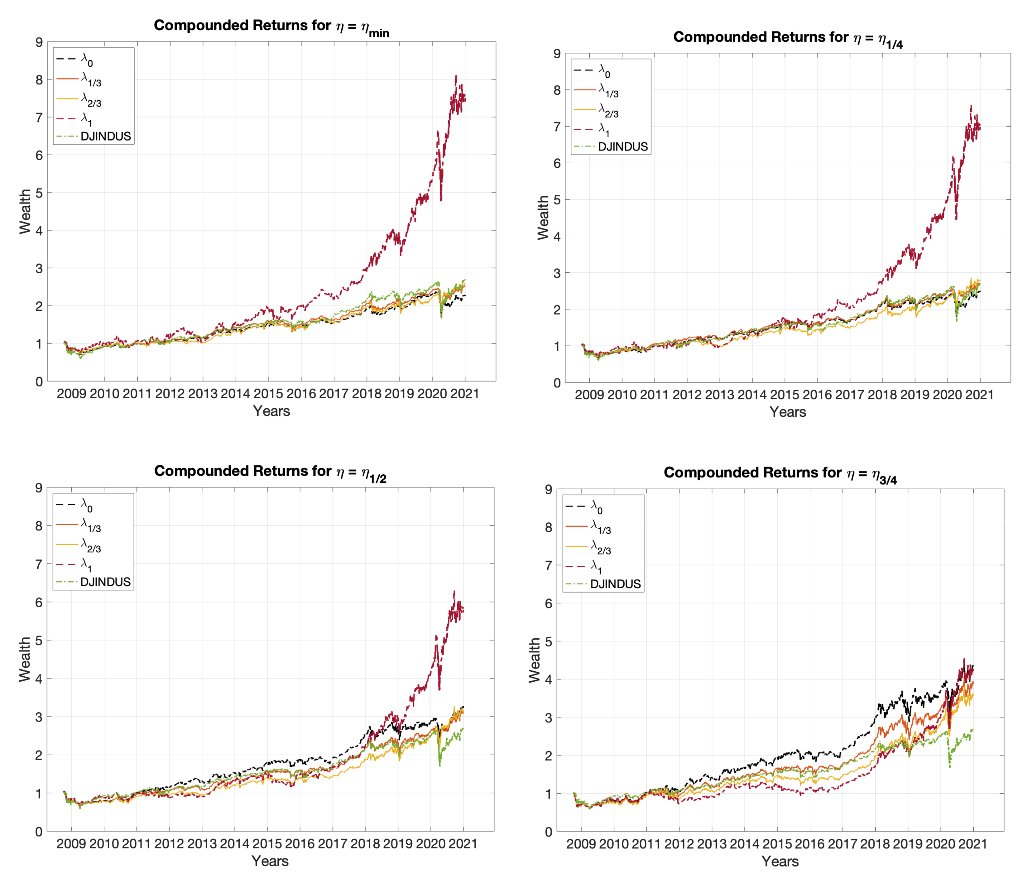
We observe that by requiring high levels of portfolio sustainability, the out-of-sample performances of the Mean-Variance-ESG portfolios typically tend to improve for each target level of the portfolio return . This behavior is most evident when low levels of the target expected return are chosen, i.e., when portfolio diversification tends to be higher. Indeed, when , the Pareto-optimal portfolios with high levels of (namely and ) achieve the best results in terms of almost all performance measures. This performance behavior can also be observed from the trend of the cumulative out-of-sample portfolio returns, reported in Figure 6. The portfolio strategies with the highest portfolio sustainability show the best performance, especially in recent years. This is most significant for low levels of the required portfolio return (namely and ), where the sustainable strategies (i.e., those with ) can reach cumulative returns almost four times higher than those of other efficient portfolios.
In Table 3 we show some statistics of ROI based on a 3-years time horizon (i.e., in Expression (7) we fix equal to 750 days) for all the portfolio strategies analyzed. Again, we can observe that the most sustainable portfolio strategies provide the best performances in terms of mean, 25%, 75%, and 95% percentile of ROI, for levels of portfolio expected return .
4.2.2. Computational Results for DowJones with Setup Split
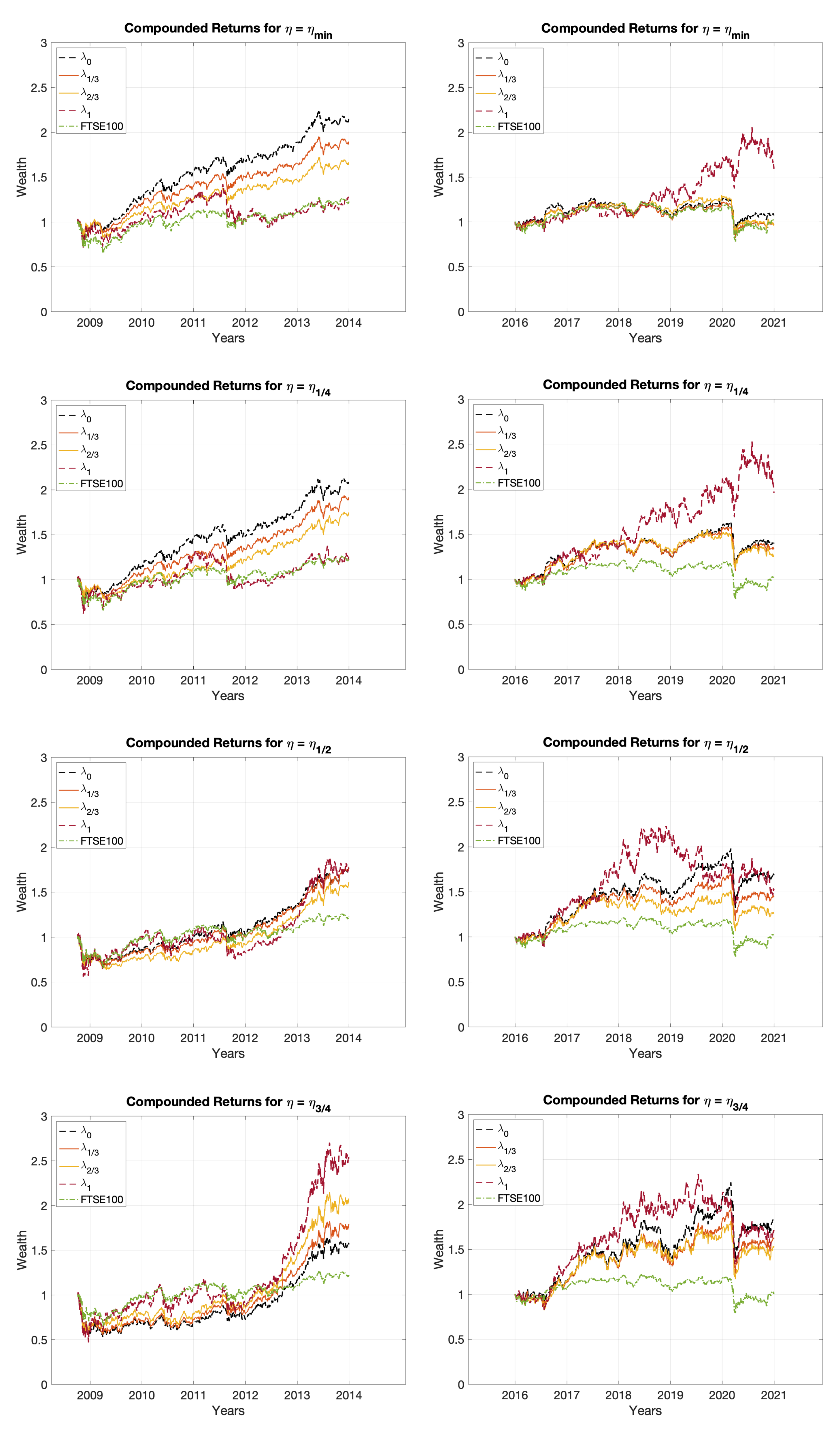
In Table 4, we show the out-of-sample performance results obtained by the 16 Mean-Variance-ESG efficient portfolios, using Setup Split, that is dividing the entire length of the time series into two non-overlapping subperiods (see Section 4.1).
More precisely, in the first table (2006–2013) we report the out-of-sample performance results obtained considering the time window ranging from October 2006 to December 2013, while in the second table (2014–2020) we present Mean, Volatility, Sharpe ratio, Max Drawdown (MaxDD), Ulcer index, Turnover, and Rachev 5% ratio evaluated on the time window spanning from January 2014 to December 2020. In the third table (Rel Diff) we provide the relative changes of the out-of-sample performance results obtained in the two subperiods considered, highlighting in bold the values that have increased or decreased by more than 50%.
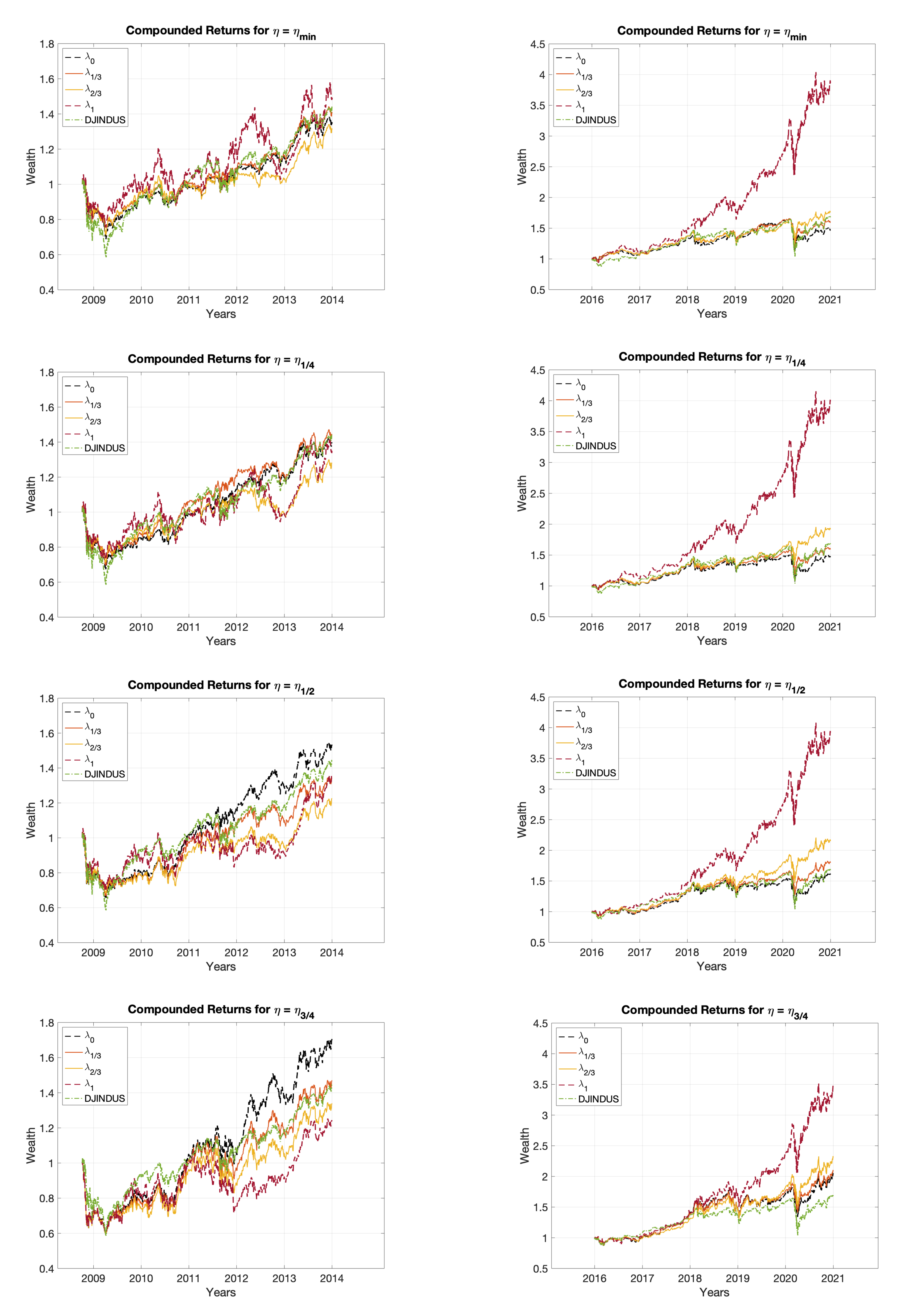
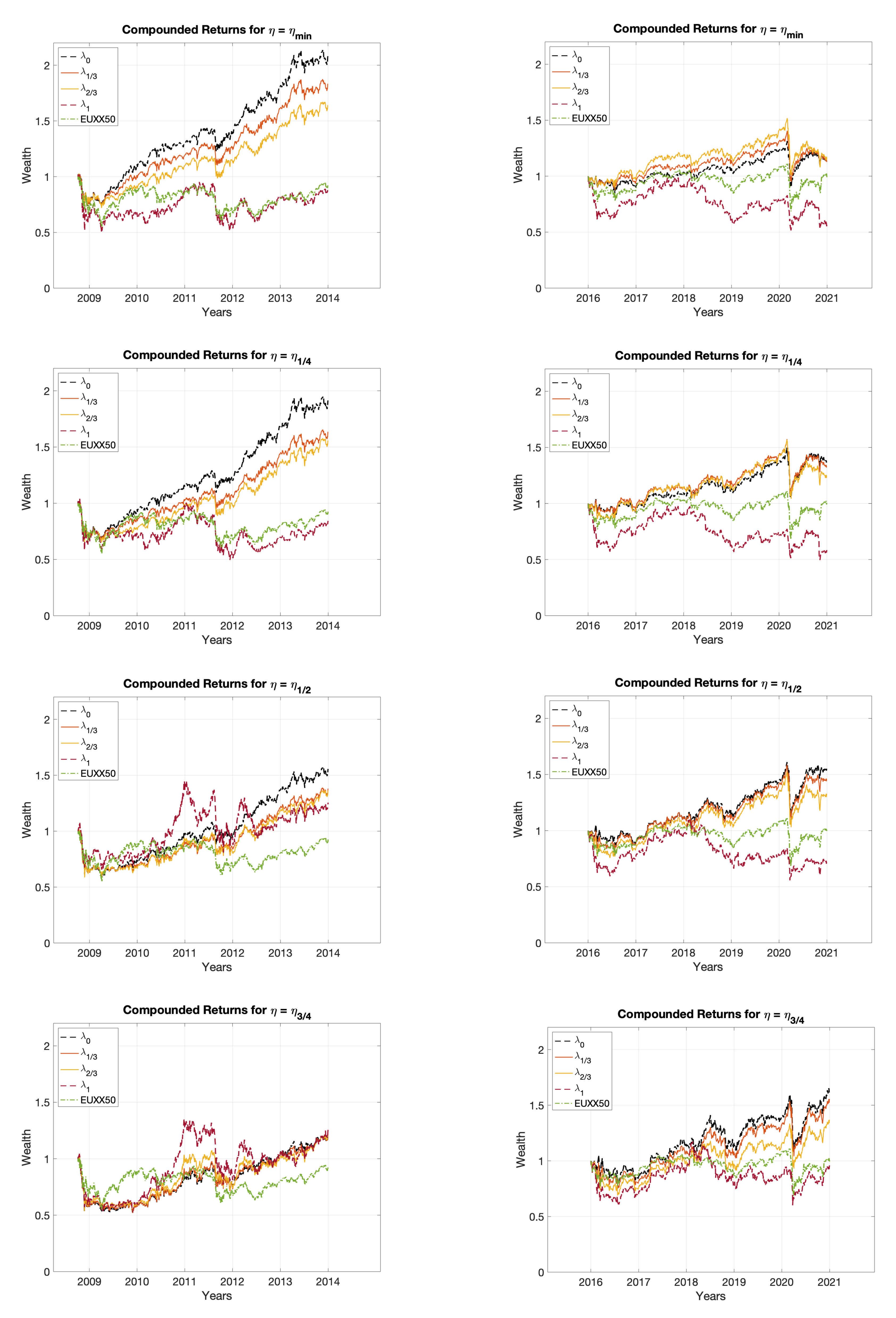
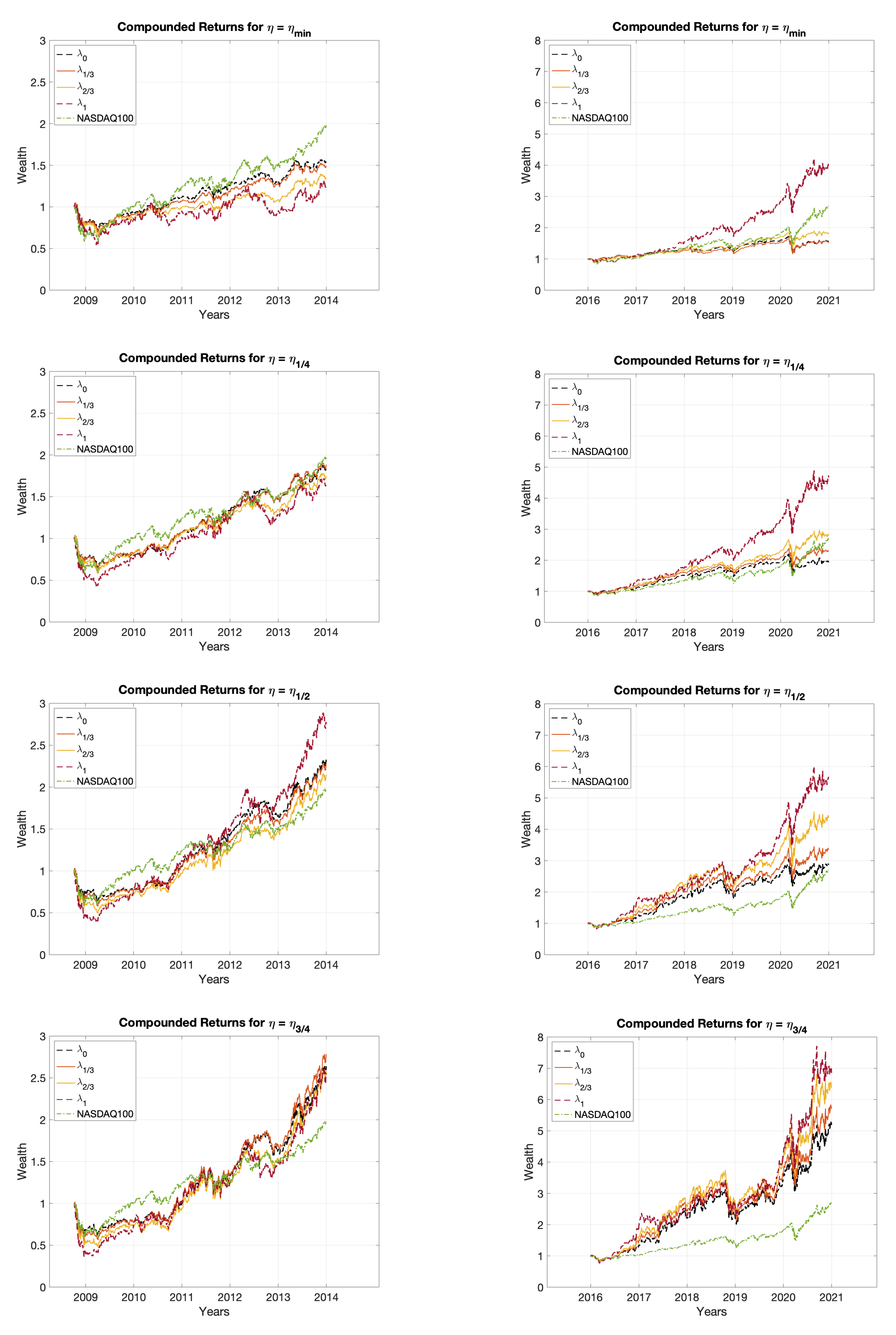
Moving from 2006–2013 to 2014–2020, we can observe remarkable improvements in the performances of the efficient portfolios requiring high target levels of the portfolio ESG. More specifically, focusing on the first subperiod, it seems that the Mean-Variance-ESG optimal portfolios do not show a clear behavioral pattern, while, in the second time window, portfolios with high levels of , namely and , typically generate better performances for every target level of the portfolio expected return . These findings are also confirmed by looking at the time evolution of the cumulative out-of-sample portfolio returns, shown in Figure 7, where we note a significantly distinct trend between the two time windows. Indeed, in the second subperiod, the most sustainable portfolio strategies clearly dominate the other optimal portfolios in terms of cumulative returns.
In Table 5 we report some summary statistics of ROI based on a 3-years time horizon for all the portfolio strategies analyzed. Again, these results seem to confirm what was previously highlighted, namely that the Pareto-optimal portfolios with the highest ESG target levels show a significant improvement in terms of profitability in the second subperiod.
From these empirical findings we can highlight two main remarks. On the one hand, as also discussed in Bermejo et al. [11], the ESG impact on the portfolio selection process typically leads to favorable and stable financial performances. This is particularly evident in the past seven years. In fact, it seems that there is a regime change in terms of profitability–sustainability around 2015, when the second commitment period of the Kyoto Protocol started and when the Paris COP21 agreement was signed. Before 2014, portfolio performances seem to show no benefits from sustainability-focused strategies, while after 2014, the ESG impact on profitability is evident. On the other hand, we can note that the sustainability-focused strategies continue to show positive effects on the financial markets even during the recent COVID-19 pandemic crisis. As also highlighted by Nofsinger and Varma [13], the positive socially responsible actions of companies could make them more profitable even in times of crisis.
4.2.3. Computational Results for EuroStoxx50 with Setup Entire
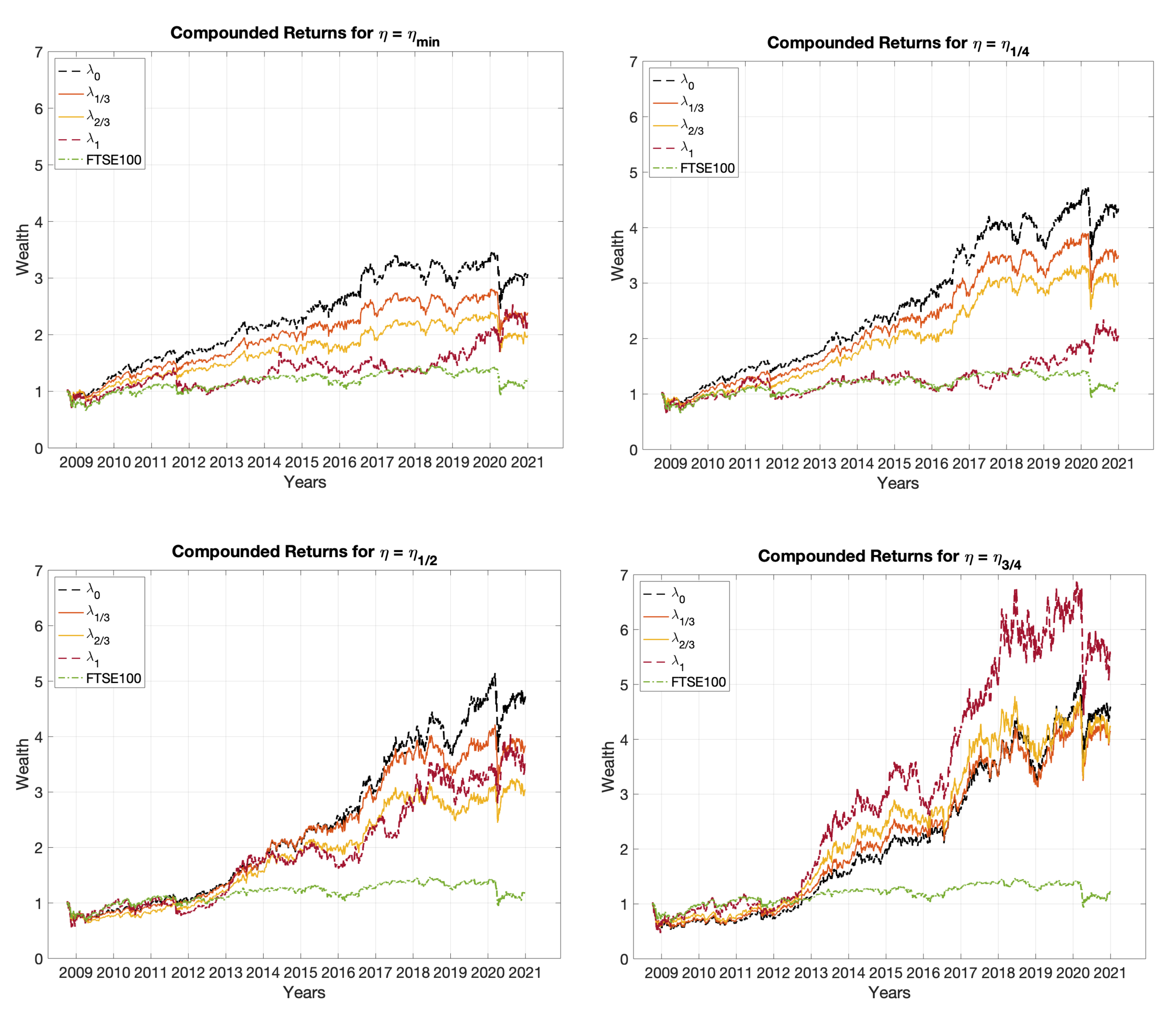
In Table 6, we provide the out-of-sample performance results obtained by the 16 analyzed portfolio strategies for EuroStoxx50, with Setup Entire.
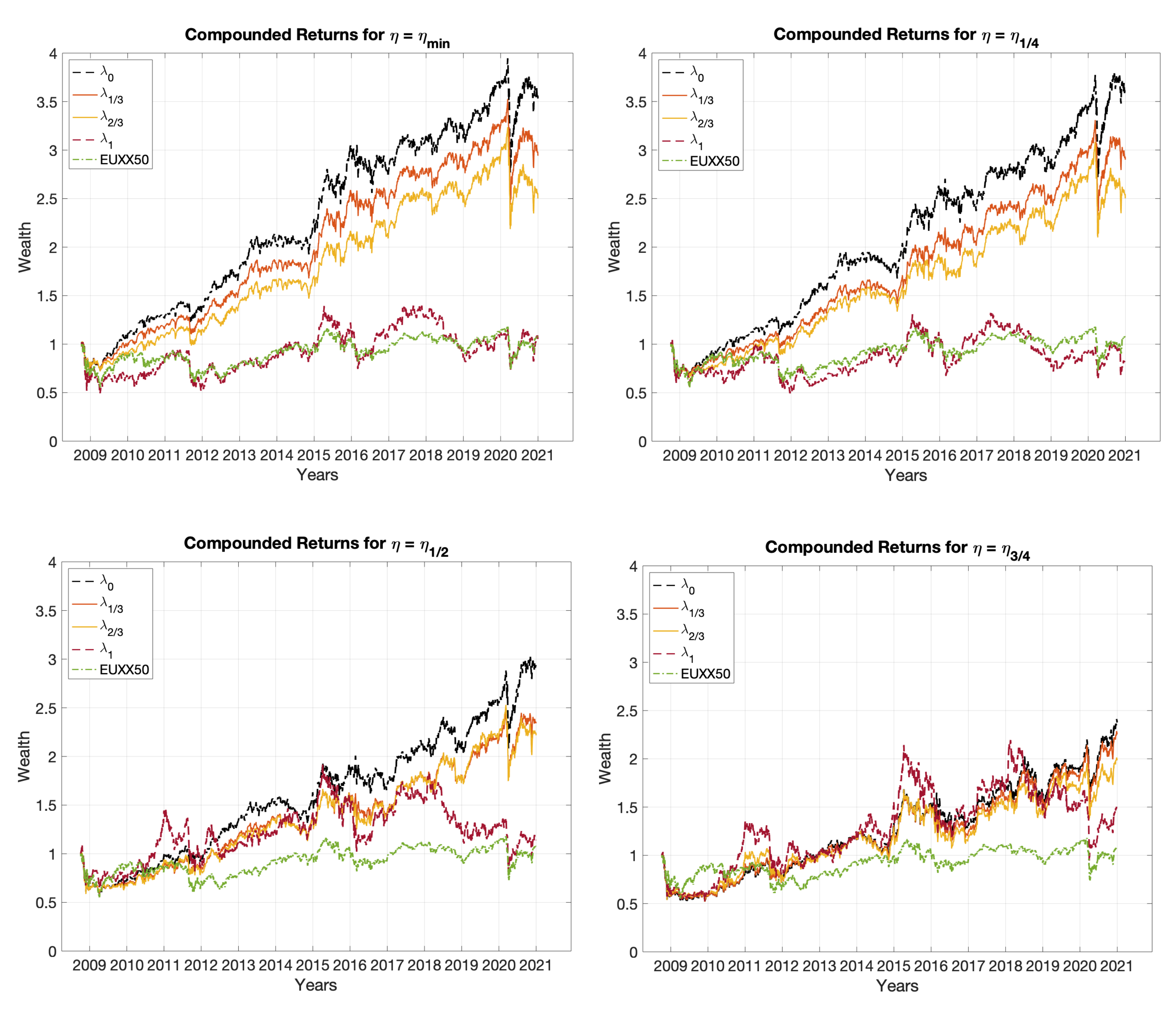
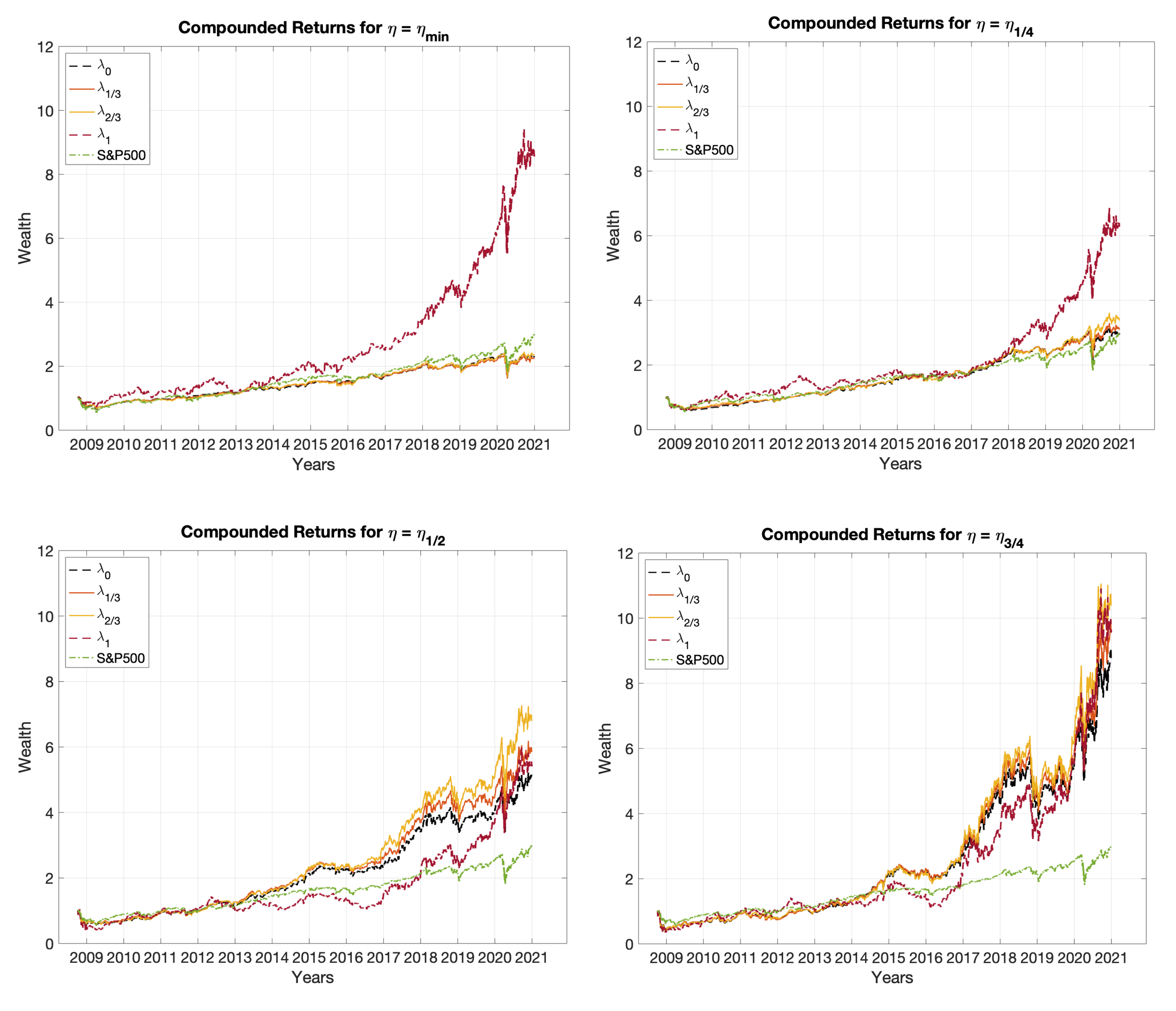
In this case, we can note that requiring high levels of the portfolio ESG generally worsens the portfolio performances for each target level of the portfolio expected return . This behavior can be also observed from the time evolution of the cumulative out-of-sample portfolio returns, reported in Figure 8, where the Mean-Variance portfolios (i.e., the Mean-Variance-ESG portfolios with ) typically show better performance than the other strategies, particularly for low values of .
In Table 7 we also provide some summary statistics of ROI based on a 3-years time horizon for all the portfolio strategies analyzed. Again, we can observe that the least sustainable portfolio strategies provide the best performances, for all the levels of target portfolio return .
4.2.4. Computational Results for EuroStoxx50 with Setup Split
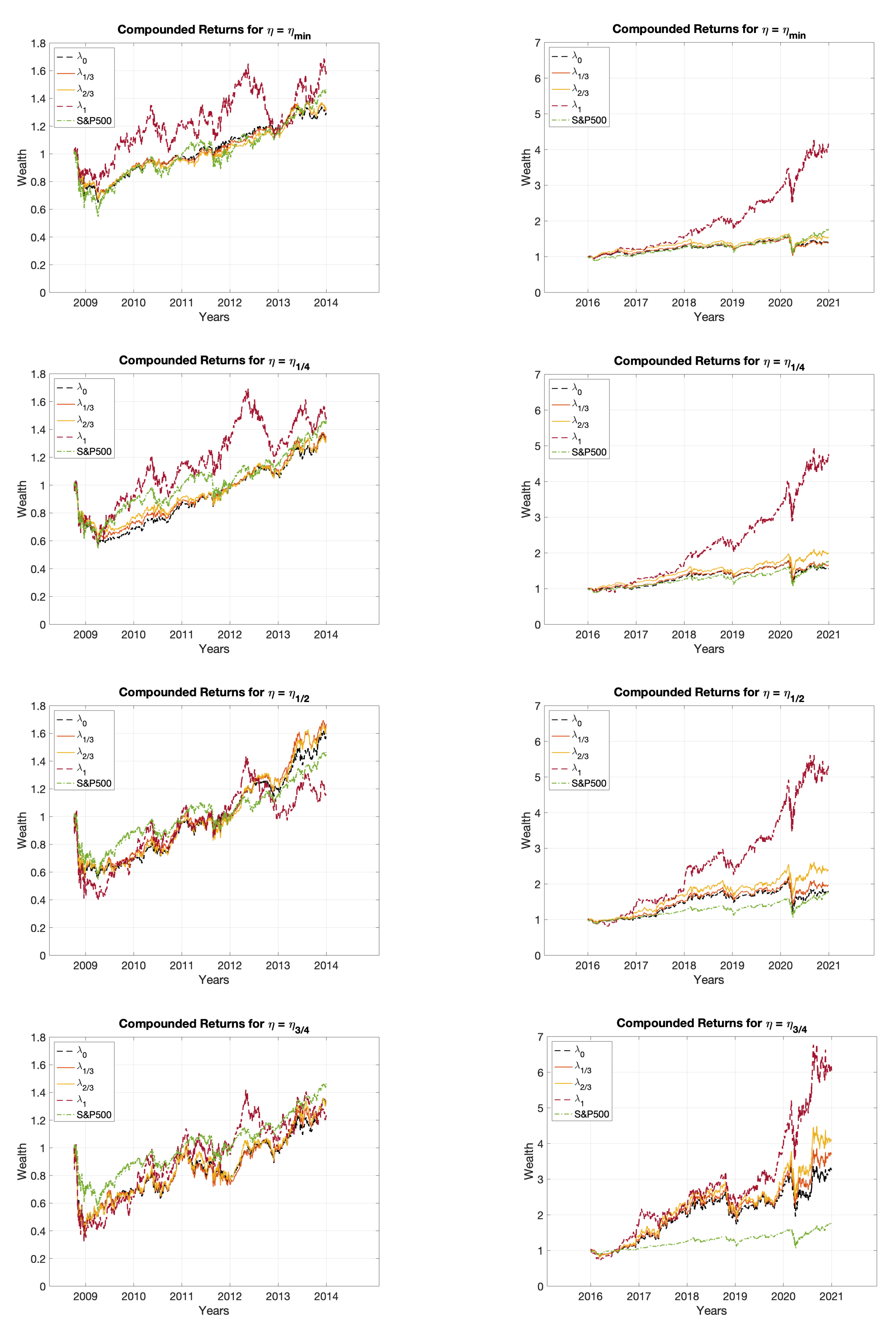
In Table 8, we report the out-of-sample performance results obtained by the 16 Mean-Variance-ESG efficient portfolios, dividing the entire length of the time series into two non-overlapping subperiods. More precisely, the first table (2006–2013) show the results obtained on the time window ranging from October 2006 to December 2013, while the second table (2014–2020) presents the out-of-sample portfolio performances evaluated on the time window spanning from January 2014 to December 2020. The third table (Rel Diff) provides the relative changes of the results obtained in the two different subperiods.
Here, we can observe that the behavioral pattern of the Mean-Variance-ESG optimal portfolios is quite similar between the two time windows analyzed. It seems that adopting high sustainable portfolio strategies generally leads to worse financial performances. Moreover, the relative differences in performance values between the two subperiods show that the optimal portfolios with low levels of ESG targets (namely with ) are the only ones that allow achieving positive changes, especially for high target return levels . This behavior can also be observed from the trend of the cumulative out-of-sample portfolio returns, reported in Figure 9.
In Table 9 we show some summary statistics of ROI based on a 3-years time horizon for all the portfolio strategies analyzed.
Although all portfolio strategies reach poor performances in the 2014–2020 subperiod, we observe that the optimal portfolios with low levels of ESG target perform better than the other approaches.
To provide an overall view of the performance of the Mean-Variance-ESG efficient portfolios, in Table 10 we report aggregate results for all the five datasets listed in Table 1. For each dataset, both using Setup Entire and Setup Split we show in green the periods where the most sustainable strategies appear to be preferable, while in blue we mark the periods where generally the least sustainable portfolios are those that provide better performance. We can observe that the US markets generally show a regime change between the two time windows analyzed. More precisely, it seems that the optimal portfolios with low ESG values generally achieve better performances in the first subperiod (2006–2013), while portfolios with high ESG target typically lead to reach better results in the second subperiod (2014–2020). On the other hand, in European markets, in particular, in the Euro Stoxx 50, the portfolio performances do not seem to be affected by imposing ESG constraints, as also pointed out by La Torre et al. [14].
5. Conclusions
We presented an extensive empirical analysis on five real-world datasets involving major equity markets, in which we investigated the in-sample and out-of-sample effects of ESG rating on the portfolio selection process. More precisely, we provided the performance of the 16 Mean-Variance-ESG efficient portfolios, obtained by solving a tri-objective portfolio optimization model, where the portfolio risk is minimized, while the portfolio expected return and the portfolio sustainability are maximized. Furthermore, to better examine the ESG impact on portfolio performance and to capture possible effects of SRI regulatory developments over the past 15 years, we conducted the out-of-sample performance analysis using both the full length of data available and the two non-overlapping subperiods of it.
When analyzing the entire period, from 2006 to 2020, we observed that only in the S&P500 and Dow Jones datasets the most sustainable portfolio strategies show better financial performances. Then, there does not appear to be a link between SRI regulatory developments and the ESG impact on portfolio profitability; however, when we separately considered the two subperiods, namely 2006–2013 and 2014–2020, we noted different regimes in terms of profitability–sustainability. Before 2014 the least sustainable portfolios provided better results on four out of five datasets. After 2014, when the second commitment period of the Kyoto Protocol started and when the Paris COP21 agreement was signed, the ESG impact on portfolio profitability became significant on four out of five datasets.
Author Contributions
Conceptualization, F.C.; methodology, F.C. and M.L.M.; software, F.C. and M.L.M.; validation, F.C. and M.L.M.; formal analysis, F.C. and M.L.M.; investigation, F.C. and M.L.M.; resources, A.C.; data curation, F.C. and M.L.M.; writing—original draft preparation, F.C., M.L.M., and A.C.; visualization, F.C. and M.L.M. All authors have read and agreed to the published version of the manuscript.
Funding
This research has been supported by the project “FinTech: the influence of enabling technologies on the future of the financial markets” funded by the Italian Ministry of Education, Universities and Research (MIUR)—PRIN 2017. Project Code: 20177WC4KE.
Institutional Review Board Statement
Not applicable.
Informed Consent Statement
Not applicable.
Data Availability Statement
Publicly available datasets were analyzed in this study. These data can be found here: https://host.uniroma3.it/docenti/cesarone/DataSets.htm (accessed on 10 February 2022).
Conflicts of Interest
The authors declare no conflict of interest. The funders had no role in the design of the study; in the collection, analyses, or interpretation of data; in the writing of the manuscript, or in the decision to publish the results.
Appendix A. Additional Out-of-Sample Performance Results
For the sake of completeness, we report here the out-of-sample performance results, obtained from the remaining datasets listed in Table 1. More precisely, in Table A1, Table A2, Table A3 and Table A4 and in Figure A1 and Figure A2, we present the computational results for the FTSE100 dataset. In Table A5, Table A6, Table A7 and Table A8 and in Figure A3 and Figure A4, we provide the computational results for the NASDAQ100 dataset. Finally, in Table A9, Table A10, Table A11 and Table A12 and in Figure A5 and Figure A6, we show the computational results for the S&P500 dataset.

Table A1.
Out-of-sample performance results for FTSE100.
| Mean | 0.0391% | 0.0313% | 0.0261% | 0.0374% | 0.0504% | 0.0438% | 0.0398% | 0.0359% | 0.0548% | 0.0485% | 0.0423% | 0.0559% | 0.0592% | 0.0565% | 0.0583% | 0.0748% |
| Volatility | 0.0092 | 0.0093 | 0.0098 | 0.0158 | 0.0096 | 0.0097 | 0.0103 | 0.0163 | 0.0112 | 0.0114 | 0.0123 | 0.0182 | 0.0151 | 0.0155 | 0.0163 | 0.0207 |
| Sharpe | 0.0427 | 0.0337 | 0.0267 | 0.0237 | 0.0527 | 0.0451 | 0.0388 | 0.0220 | 0.0488 | 0.0426 | 0.0345 | 0.0307 | 0.0391 | 0.0366 | 0.0358 | 0.0361 |
| MaxDD | −0.2903 | −0.2970 | −0.2980 | −0.3443 | −0.2794 | −0.2753 | −0.2548 | −0.4014 | −0.3484 | −0.3422 | −0.3852 | −0.4655 | −0.4790 | −0.4596 | −0.4482 | −0.5451 |
| Ulcer | 0.0632 | 0.0654 | 0.0701 | 0.1520 | 0.0622 | 0.0639 | 0.0635 | 0.1430 | 0.0985 | 0.1027 | 0.1342 | 0.1327 | 0.1853 | 0.1716 | 0.1534 | 0.1441 |
| Turnover | 0.2031 | 0.2139 | 0.2131 | 0.3783 | 0.3369 | 0.3624 | 0.3998 | 0.5588 | 0.4924 | 0.5161 | 0.5637 | 0.7290 | 0.6087 | 0.6278 | 0.6415 | 0.7136 |
| Rachev | 0.9675 | 0.9609 | 0.9820 | 1.0125 | 0.9623 | 0.9439 | 0.9741 | 0.9757 | 0.9395 | 0.9437 | 0.9464 | 1.0005 | 0.9319 | 0.9297 | 0.9627 | 1.0313 |
Table A2.
Summary statistics of ROI based on a 3-years time horizon for FTSE100.
| Approach | Index | ||||||||||||||||
| Mean | 11% | 33% | 27% | 23% | 20% | 49% | 44% | 42% | 21% | 65% | 60% | 52% | 52% | 78% | 74% | 76% | 89% |
| Vol | 14% | 22% | 18% | 15% | 22% | 20% | 18% | 17% | 22% | 23% | 29% | 30% | 34% | 38% | 45% | 53% | 62% |
| 5perc | −18% | −7% | −11% | −10% | −11% | 6% | 1% | 2% | −11% | 18% | 5% | 4% | 5% | 22% | 14% | 6% | 12% |
| 25perc | 5% | 20% | 17% | 16% | 5% | 39% | 37% | 34% | 5% | 50% | 42% | 32% | 25% | 52% | 44% | 42% | 42% |
| 75perc | 18% | 45% | 37% | 32% | 33% | 62% | 57% | 53% | 36% | 83% | 79% | 76% | 78% | 106% | 108% | 113% | 131% |
| 95perc | 31% | 74% | 57% | 47% | 65% | 75% | 66% | 65% | 62% | 97% | 106% | 103% | 114% | 145% | 154% | 170% | 213% |
Figure A1.
Cumulative out-of-sample portfolio returns using different levels of for FTSE100.

Table A3.
Out-of-sample performance results over two non-overlapping subperiods for FTSE100.
| Mean | 0.0601% | 0.0513% | 0.0426% | 0.0338% | 0.0592% | 0.0528% | 0.0471% | 0.0345% | 0.0492% | 0.0501% | 0.0445% | 0.0660% | 0.0488% | 0.0587% | 0.0714% | 0.0984% | 2006–2013 |
| Volatility | 0.0097 | 0.0100 | 0.0107 | 0.0175 | 0.0103 | 0.0106 | 0.0115 | 0.0189 | 0.0125 | 0.0128 | 0.0141 | 0.0221 | 0.0176 | 0.0180 | 0.0192 | 0.0249 | |
| Sharpe | 0.0620 | 0.0515 | 0.0398 | 0.0193 | 0.0575 | 0.0497 | 0.0409 | 0.0182 | 0.0394 | 0.0391 | 0.0316 | 0.0299 | 0.0278 | 0.0325 | 0.0373 | 0.0395 | |
| MaxDD | −0.2292 | −0.2321 | −0.2375 | −0.3443 | −0.2597 | −0.2600 | −0.2548 | −0.4014 | −0.3484 | −0.3422 | −0.3852 | −0.4655 | −0.4790 | −0.4596 | −0.4482 | −0.5451 | |
| Ulcer | 0.0449 | 0.0459 | 0.0557 | 0.1696 | 0.0637 | 0.0680 | 0.0731 | 0.1705 | 0.1309 | 0.1362 | 0.1843 | 0.1632 | 0.2623 | 0.2376 | 0.2001 | 0.1758 | |
| Turnover | 0.1602 | 0.1831 | 0.2064 | 0.4468 | 0.3771 | 0.4155 | 0.4470 | 0.5359 | 0.5840 | 0.5853 | 0.6208 | 0.7107 | 0.7382 | 0.7356 | 0.7006 | 0.6879 | |
| Rachev | 0.9733 | 0.9955 | 1.0250 | 0.9701 | 0.9658 | 0.9523 | 0.9631 | 0.9310 | 0.9448 | 0.9572 | 0.9551 | 0.9663 | 0.9371 | 0.9240 | 0.9502 | 1.0215 | |
| Mean | 0.0100% | 0.0023% | 0.0016% | 0.0466% | 0.0303% | 0.0267% | 0.0212% | 0.0618% | 0.0457% | 0.0338% | 0.0239% | 0.0431% | 0.0553% | 0.0463% | 0.0425% | 0.0543% | 2014–2020 |
| Volatility | 0.0090 | 0.0090 | 0.0093 | 0.0150 | 0.0094 | 0.0093 | 0.0094 | 0.0147 | 0.0106 | 0.0105 | 0.0111 | 0.0154 | 0.0136 | 0.0136 | 0.0141 | 0.0167 | |
| Sharpe | 0.0111 | 0.0025 | 0.0017 | 0.0311 | 0.0323 | 0.0288 | 0.0224 | 0.0421 | 0.0430 | 0.0322 | 0.0216 | 0.0280 | 0.0408 | 0.0340 | 0.0302 | 0.0326 | |
| MaxDD | −0.3141 | −0.3311 | −0.3295 | −0.2249 | −0.3275 | −0.3091 | −0.2805 | −0.2249 | −0.3343 | −0.3139 | −0.2991 | −0.3949 | −0.3877 | −0.3771 | −0.3578 | −0.4283 | |
| Ulcer | 0.0936 | 0.1026 | 0.1059 | 0.0733 | 0.0823 | 0.0790 | 0.0779 | 0.0679 | 0.0873 | 0.0857 | 0.0938 | 0.1501 | 0.1179 | 0.1160 | 0.1082 | 0.1419 | |
| Turnover | 0.2473 | 0.2391 | 0.2124 | 0.3147 | 0.3178 | 0.3302 | 0.3811 | 0.4038 | 0.4440 | 0.4890 | 0.5461 | 0.6344 | 0.4790 | 0.5128 | 0.5371 | 0.6062 | |
| Rachev | 0.9045 | 0.8703 | 0.8818 | 1.0507 | 0.8993 | 0.8887 | 0.9319 | 1.1117 | 0.8773 | 0.8467 | 0.8790 | 1.0012 | 0.8583 | 0.8727 | 0.8968 | 0.9978 | |
| Mean | −83% | −96% | −96% | 38% | −49% | −49% | −55% | 79% | −7% | −33% | −46% | −35% | 13% | −21% | −40% | −45% | Rel Diff |
| Volatility | −7% | −10% | −13% | −14% | −9% | −13% | −18% | −22% | −15% | −18% | −21% | −30% | −23% | −24% | −27% | −33% | |
| Sharpe | −82% | −95% | −96% | 61% | −44% | −42% | −45% | 131% | 9% | −18% | −32% | −6% | 47% | 5% | −19% | −18% | |
| MaxDD | 37% | 43% | 39% | −35% | 26% | 19% | 10% | −44% | −4% | −8% | −22% | −15% | −19% | −18% | −20% | −21% | |
| Ulcer | 109% | 124% | 90% | −57% | 29% | 16% | 7% | −60% | −33% | −37% | −49% | −8% | −55% | −51% | −46% | −19% | |
| Turnover | 54% | 31% | 3% | −30% | −16% | −21% | −15% | −25% | −24% | −16% | −12% | −11% | −35% | −30% | −23% | −12% | |
| Rachev | −7% | −13% | −14% | 8% | −7% | −7% | −3% | 19% | −7% | −12% | −8% | 4% | −8% | −6% | −6% | −2% | |
Table A4.
Summary statistics of ROI based on a 3-years time horizon over two non-overlapping subperiods for FTSE100.
Table A4.
Summary statistics of ROI based on a 3-years time horizon over two non-overlapping subperiods for FTSE100.
| Approach | Index | |||||||||||||||||
|---|---|---|---|---|---|---|---|---|---|---|---|---|---|---|---|---|---|---|
| Mean | 21% | 55% | 45% | 38% | 10% | 57% | 50% | 45% | 16% | 58% | 57% | 57% | 37% | 70% | 80% | 87% | 80% | 2006–2013 |
| Vol | 12% | 17% | 12% | 11% | 12% | 13% | 9% | 10% | 11% | 17% | 21% | 25% | 32% | 44% | 47% | 55% | 54% | |
| 5perc | 8% | 35% | 30% | 25% | −5% | 39% | 39% | 27% | −2% | 30% | 23% | 16% | 3% | 12% | 15% | 22% | 19% | |
| 25perc | 12% | 40% | 34% | 30% | 2% | 47% | 44% | 40% | 11% | 49% | 47% | 44% | 11% | 39% | 47% | 43% | 37% | |
| 75perc | 28% | 70% | 54% | 42% | 15% | 69% | 56% | 52% | 22% | 68% | 77% | 80% | 68% | 115% | 130% | 147% | 137% | |
| 95perc | 47% | 83% | 67% | 62% | 36% | 80% | 68% | 61% | 34% | 85% | 88% | 94% | 94% | 141% | 155% | 178% | 174% | |
| Approach | Index | |||||||||||||||||
| Mean | −1% | 0% | −1% | 3% | 48% | 18% | 18% | 17% | 65% | 35% | 23% | 13% | 42% | 47% | 36% | 33% | 54% | 2014–2020 |
| Vol | 15% | 12% | 14% | 17% | 15% | 15% | 17% | 19% | 13% | 20% | 19% | 18% | 42% | 24% | 23% | 26% | 49% | |
| 5perc | −23% | −20% | −23% | −21% | 28% | −8% | −8% | −11% | 46% | 4% | −7% | −15% | −10% | 9% | −1% | −8% | −11% | |
| 25perc | −17% | −10% | −16% | −16% | 36% | 2% | −1% | −5% | 57% | 12% | 1% | −6% | 8% | 22% | 14% | 8% | 6% | |
| 75perc | 12% | 10% | 10% | 17% | 57% | 30% | 31% | 34% | 73% | 50% | 40% | 30% | 84% | 64% | 51% | 55% | 104% | |
| 95perc | 19% | 17% | 17% | 23% | 75% | 37% | 38% | 42% | 89% | 58% | 46% | 37% | 115% | 80% | 69% | 71% | 125% | |
| Approach | Index | |||||||||||||||||
| Mean | −104% | −100% | −102% | −91% | 364% | −69% | −65% | −63% | 297% | −40% | −60% | −77% | 14% | −34% | −55% | −62% | −32% | Rel Diff |
| Vol | 26% | −30% | 14% | 57% | 21% | 16% | 84% | 97% | 15% | 16% | −8% | −28% | 30% | −46% | −52% | −52% | −10% | |
| 5perc | −399% | −158% | −177% | −182% | 619% | −120% | −121% | −141% | 2033% | −87% | −131% | −192% | −455% | −25% | −108% | −137% | −157% | |
| 25perc | −242% | −126% | −147% | −154% | 1730% | −95% | −102% | −112% | 442% | −75% | −98% | −113% | −32% | −43% | −70% | −81% | −85% | |
| 75perc | −57% | −86% | −82% | −60% | 283% | −56% | −44% | −34% | 226% | −27% | −48% | −63% | 23% | −44% | −61% | −62% | −24% | |
| 95perc | −60% | −80% | −75% | −63% | 110% | −54% | −45% | −31% | 159% | −32% | −47% | −61% | 22% | −43% | −56% | −60% | −28% | |
Figure A2.
Cumulative out-of-sample portfolio returns using different levels of over two non-overlapping subperiods for FTSE100.
Figure A2.
Cumulative out-of-sample portfolio returns using different levels of over two non-overlapping subperiods for FTSE100.

Table A5.
Out-of-sample performance results for NASDAQ100.
| Mean | 0.0430% | 0.0419% | 0.0443% | 0.0770% | 0.0574% | 0.0607% | 0.0666% | 0.0829% | 0.0822% | 0.0839% | 0.0904% | 0.1147% | 0.1120% | 0.1169% | 0.1192% | 0.1264% |
| Volatility | 0.0101 | 0.0103 | 0.0111 | 0.0178 | 0.0112 | 0.0115 | 0.0127 | 0.0175 | 0.0141 | 0.0146 | 0.0157 | 0.0193 | 0.0187 | 0.0191 | 0.0199 | 0.0226 |
| Sharpe | 0.0424 | 0.0405 | 0.0398 | 0.0432 | 0.0513 | 0.0529 | 0.0524 | 0.0475 | 0.0583 | 0.0574 | 0.0576 | 0.0594 | 0.0600 | 0.0614 | 0.0598 | 0.0559 |
| MaxDD | −0.3250 | −0.3365 | −0.3828 | −0.4849 | −0.3716 | −0.3871 | −0.4467 | −0.5764 | −0.3891 | −0.4432 | −0.5160 | −0.6053 | −0.4108 | −0.4566 | −0.5229 | −0.6367 |
| Ulcer | 0.0757 | 0.0792 | 0.0899 | 0.1320 | 0.1034 | 0.0980 | 0.1076 | 0.1546 | 0.1149 | 0.1223 | 0.1432 | 0.1614 | 0.1311 | 0.1383 | 0.1611 | 0.1899 |
| Turnover | 0.1339 | 0.1522 | 0.1771 | 0.1786 | 0.3462 | 0.3560 | 0.3676 | 0.3478 | 0.4716 | 0.4937 | 0.4688 | 0.3871 | 0.5006 | 0.5168 | 0.5197 | 0.5171 |
| Rachev | 0.9270 | 0.9274 | 0.9264 | 1.0222 | 0.9240 | 0.9268 | 0.9371 | 0.9831 | 0.9514 | 0.9450 | 0.9507 | 0.9876 | 0.9866 | 0.9902 | 0.9872 | 0.9974 |
Table A6.
Summary statistics of ROI based on a 3-years time horizon for NASDAQ100.
| Approach | Index | ||||||||||||||||
| Mean | 61% | 42% | 40% | 43% | 73% | 65% | 66% | 71% | 91% | 95% | 97% | 109% | 146% | 125% | 134% | 144% | 154% |
| Vol | 16% | 11% | 11% | 11% | 47% | 18% | 17% | 21% | 56% | 27% | 30% | 39% | 62% | 33% | 38% | 47% | 71% |
| 5perc | 39% | 21% | 24% | 21% | 6% | 38% | 38% | 38% | 13% | 52% | 46% | 44% | 54% | 70% | 70% | 72% | 66% |
| 25perc | 49% | 36% | 34% | 37% | 39% | 53% | 54% | 55% | 46% | 73% | 74% | 83% | 108% | 105% | 112% | 115% | 103% |
| 75perc | 70% | 49% | 48% | 50% | 108% | 73% | 76% | 88% | 145% | 116% | 120% | 134% | 180% | 146% | 158% | 168% | 185% |
| 95perc | 91% | 59% | 57% | 58% | 158% | 99% | 94% | 105% | 181% | 138% | 143% | 180% | 261% | 177% | 200% | 236% | 314% |
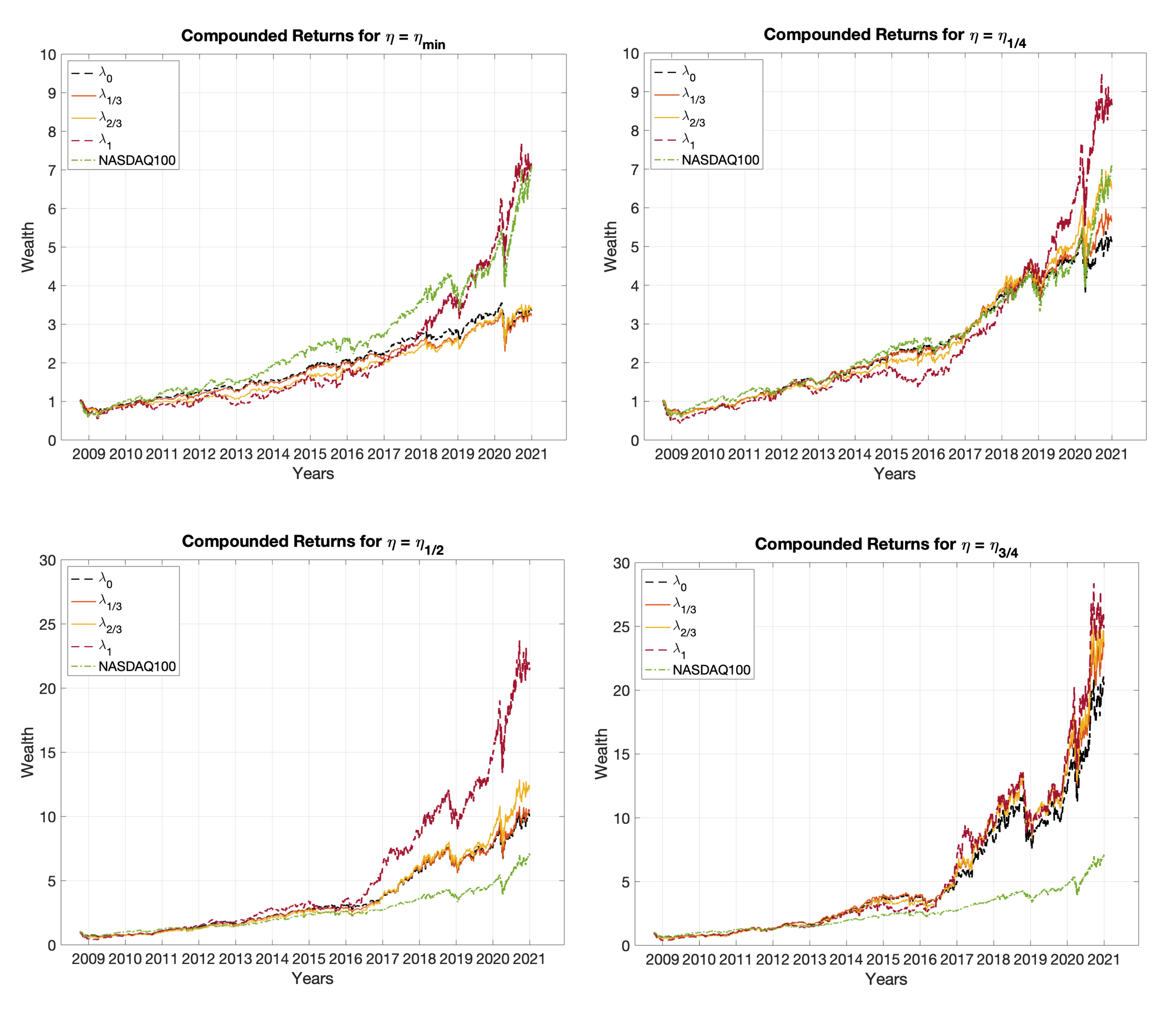
Figure A3.
Cumulative out-of-sample portfolio returns using different levels of for NASDAQ100.

Table A7.
Out-of-sample performance results over two non-overlapping subperiods for NASDAQ100.
| Mean | 0.0376% | 0.0347% | 0.0287% | 0.0343% | 0.0517% | 0.0527% | 0.0488% | 0.0534% | 0.0706% | 0.0697% | 0.0674% | 0.0950% | 0.0856% | 0.0901% | 0.0867% | 0.0936% | 2006–2013 |
| Volatility | 0.0106 | 0.0107 | 0.0117 | 0.0194 | 0.0114 | 0.0116 | 0.0129 | 0.0186 | 0.0137 | 0.0142 | 0.0154 | 0.0204 | 0.0175 | 0.0178 | 0.0189 | 0.0225 | |
| Sharpe | 0.0354 | 0.0323 | 0.0245 | 0.0177 | 0.0454 | 0.0453 | 0.0377 | 0.0287 | 0.0515 | 0.0492 | 0.0437 | 0.0465 | 0.0490 | 0.0505 | 0.0460 | 0.0416 | |
| MaxDD | −0.3145 | −0.3365 | −0.3828 | −0.4849 | −0.3716 | −0.3871 | −0.4467 | −0.5764 | −0.3891 | −0.4432 | −0.5160 | −0.6053 | −0.4108 | −0.4566 | −0.5229 | −0.6367 | |
| Ulcer | 0.0988 | 0.1078 | 0.1274 | 0.1875 | 0.1465 | 0.1401 | 0.1560 | 0.2162 | 0.1589 | 0.1694 | 0.2020 | 0.2235 | 0.1626 | 0.1759 | 0.2130 | 0.2496 | |
| Turnover | 0.1156 | 0.1568 | 0.2626 | 0.4035 | 0.2855 | 0.3448 | 0.4185 | 0.5193 | 0.4237 | 0.4938 | 0.5428 | 0.4719 | 0.5360 | 0.5850 | 0.6305 | 0.6541 | |
| Rachev | 0.9329 | 0.9286 | 0.9170 | 1.0052 | 0.9275 | 0.9149 | 0.9072 | 0.9983 | 0.9811 | 0.9564 | 0.9307 | 1.0008 | 1.0053 | 0.9840 | 0.9462 | 0.9586 | |
| Mean | 0.0382% | 0.0373% | 0.0509% | 0.1201% | 0.0570% | 0.0694% | 0.0871% | 0.1319% | 0.0918% | 0.1044% | 0.1268% | 0.1486% | 0.1467% | 0.1551% | 0.1653% | 0.1749% | 2014–2020 |
| Volatility | 0.0105 | 0.0107 | 0.0113 | 0.0172 | 0.0118 | 0.0121 | 0.0135 | 0.0173 | 0.0154 | 0.0161 | 0.0174 | 0.0191 | 0.0209 | 0.0215 | 0.0224 | 0.0240 | |
| Sharpe | 0.0363 | 0.0349 | 0.0451 | 0.0700 | 0.0484 | 0.0575 | 0.0644 | 0.0761 | 0.0594 | 0.0649 | 0.0730 | 0.0779 | 0.0701 | 0.0720 | 0.0739 | 0.0728 | |
| MaxDD | −0.3337 | −0.3011 | −0.2753 | −0.2824 | −0.2928 | −0.2720 | −0.2845 | −0.2823 | −0.2883 | −0.2980 | −0.3206 | −0.2969 | −0.3609 | −0.3798 | −0.3770 | −0.3402 | |
| Ulcer | 0.0673 | 0.0603 | 0.0485 | 0.0558 | 0.0687 | 0.0537 | 0.0499 | 0.0549 | 0.0803 | 0.0776 | 0.0744 | 0.0753 | 0.1085 | 0.1158 | 0.1157 | 0.1111 | |
| Turnover | 0.1538 | 0.1630 | 0.1270 | 0.0044 | 0.4068 | 0.3635 | 0.3092 | 0.0832 | 0.5495 | 0.5068 | 0.4152 | 0.2670 | 0.5164 | 0.4867 | 0.4348 | 0.4383 | |
| Rachev | 0.8559 | 0.8653 | 0.9105 | 1.0272 | 0.9061 | 0.9311 | 0.9700 | 1.0014 | 0.9313 | 0.9538 | 0.9793 | 0.9706 | 0.9886 | 1.0142 | 1.0329 | 1.0437 | |
| Mean | 2% | 7% | 77% | 250% | 10% | 32% | 79% | 147% | 30% | 50% | 88% | 56% | 71% | 72% | 91% | 87% | Rel Diff |
| Volatility | −1% | 0% | −4% | −11% | 3% | 4% | 5% | −7% | 13% | 14% | 12% | −7% | 20% | 21% | 19% | 7% | |
| Sharpe | 3% | 8% | 84% | 295% | 7% | 27% | 71% | 165% | 15% | 32% | 67% | 68% | 43% | 43% | 61% | 75% | |
| MaxDD | 6% | −11% | −28% | −42% | −21% | −30% | −36% | −51% | −26% | −33% | −38% | −51% | −12% | −17% | −28% | −47% | |
| Ulcer | −32% | −44% | −62% | −70% | −53% | −62% | −68% | −75% | −49% | −54% | −63% | −66% | −33% | −34% | −46% | −55% | |
| Turnover | 33% | 4% | −52% | −99% | 42% | 5% | −26% | −84% | 30% | 3% | −24% | −43% | −4% | −17% | −31% | −33% | |
| Rachev | −8% | −7% | −1% | 2% | −2% | 2% | 7% | 0% | −5% | 0% | 5% | −3% | −2% | 3% | 9% | 9% | |
Table A8.
Summary statistics of ROI based on a 3-years time horizon over two non-overlapping subperiods for NASDAQ100.
Table A8.
Summary statistics of ROI based on a 3-years time horizon over two non-overlapping subperiods for NASDAQ100.
| Approach | Index | |||||||||||||||||
|---|---|---|---|---|---|---|---|---|---|---|---|---|---|---|---|---|---|---|
| Mean | 65% | 47% | 44% | 32% | 31% | 83% | 79% | 71% | 92% | 113% | 108% | 109% | 167% | 118% | 129% | 131% | 139% | 2006–2013 |
| Vol | 21% | 12% | 11% | 12% | 24% | 18% | 17% | 20% | 41% | 25% | 24% | 27% | 50% | 28% | 28% | 32% | 44% | |
| 5perc | 38% | 33% | 32% | 15% | −5% | 57% | 54% | 48% | 45% | 71% | 67% | 62% | 103% | 73% | 84% | 82% | 69% | |
| 25perc | 50% | 38% | 37% | 25% | 11% | 71% | 70% | 59% | 60% | 103% | 98% | 99% | 135% | 101% | 114% | 115% | 111% | |
| 75perc | 79% | 56% | 51% | 39% | 44% | 97% | 90% | 81% | 120% | 132% | 124% | 126% | 202% | 135% | 144% | 150% | 170% | |
| 95perc | 103% | 64% | 60% | 52% | 74% | 104% | 103% | 104% | 167% | 141% | 139% | 149% | 259% | 162% | 176% | 186% | 216% | |
| Approach | Index | |||||||||||||||||
| Mean | 66% | 31% | 29% | 46% | 139% | 58% | 66% | 82% | 150% | 93% | 102% | 127% | 155% | 133% | 136% | 151% | 152% | 2014–2020 |
| Vol | 13% | 12% | 9% | 8% | 25% | 19% | 17% | 14% | 19% | 29% | 31% | 32% | 25% | 29% | 36% | 41% | 43% | |
| 5perc | 46% | 11% | 14% | 33% | 95% | 28% | 39% | 59% | 123% | 45% | 53% | 80% | 109% | 89% | 86% | 98% | 74% | |
| 25perc | 57% | 19% | 22% | 39% | 128% | 36% | 46% | 71% | 135% | 62% | 69% | 98% | 141% | 109% | 104% | 115% | 124% | |
| 75perc | 74% | 41% | 36% | 52% | 154% | 73% | 79% | 93% | 163% | 118% | 128% | 154% | 174% | 161% | 167% | 184% | 188% | |
| 95perc | 88% | 46% | 42% | 57% | 183% | 80% | 87% | 105% | 186% | 128% | 144% | 174% | 194% | 176% | 193% | 222% | 222% | |
| Approach | Index | |||||||||||||||||
| Mean | 2% | −34% | −35% | 43% | 353% | −30% | −17% | 16% | 64% | −18% | −6% | 16% | −7% | 14% | 6% | 15% | 10% | Rel Diff |
| Vol | −39% | 4% | −20% | −34% | 5% | 4% | −1% | −27% | −53% | 19% | 31% | 18% | −49% | 4% | 28% | 29% | −2% | |
| 5perc | 22% | −68% | −57% | 122% | 1945% | −51% | −27% | 23% | 173% | −36% | −20% | 29% | 6% | 22% | 3% | 20% | 7% | |
| 25perc | 15% | −49% | −40% | 58% | 1109% | −50% | −34% | 19% | 123% | −40% | −29% | −1% | 4% | 8% | −9% | 0% | 13% | |
| 75perc | −6% | −26% | −30% | 34% | 248% | −25% | −12% | 15% | 35% | −11% | 3% | 22% | −14% | 20% | 16% | 23% | 10% | |
| 95perc | −15% | −28% | −31% | 11% | 148% | −24% | −15% | 1% | 12% | −9% | 4% | 17% | −25% | 8% | 10% | 19% | 3% | |
Figure A4.
Cumulative out-of-sample portfolio returns using different levels of over two non-overlapping subperiods for NASDAQ100.
Figure A4.
Cumulative out-of-sample portfolio returns using different levels of over two non-overlapping subperiods for NASDAQ100.

Table A9.
Out-of-sample performance results for S&P500.
| Mean | 0.0301% | 0.0294% | 0.0312% | 0.0812% | 0.0388% | 0.0405% | 0.0437% | 0.0727% | 0.0599% | 0.0650% | 0.0713% | 0.0776% | 0.0877% | 0.0914% | 0.0964% | 0.1041% |
| Volatility | 0.0093 | 0.0093 | 0.0095 | 0.0166 | 0.0101 | 0.0101 | 0.0107 | 0.0174 | 0.0136 | 0.0140 | 0.0151 | 0.0220 | 0.0197 | 0.0202 | 0.0214 | 0.0256 |
| Sharpe | 0.0325 | 0.0316 | 0.0326 | 0.0490 | 0.0385 | 0.0399 | 0.0410 | 0.0418 | 0.0440 | 0.0466 | 0.0474 | 0.0352 | 0.0445 | 0.0451 | 0.0451 | 0.0407 |
| MaxDD | −0.3721 | −0.3488 | −0.3441 | −0.3235 | −0.4479 | −0.4198 | −0.3866 | −0.4506 | −0.4812 | −0.4693 | −0.4697 | −0.6152 | −0.6370 | −0.6410 | −0.6457 | −0.6890 |
| Ulcer | 0.0896 | 0.0845 | 0.0883 | 0.1054 | 0.1465 | 0.1302 | 0.1207 | 0.1256 | 0.1451 | 0.1348 | 0.1445 | 0.1998 | 0.1805 | 0.1840 | 0.1838 | 0.2162 |
| Turnover | 0.2548 | 0.2570 | 0.2251 | 0.1766 | 0.4716 | 0.4924 | 0.4658 | 0.3996 | 0.6002 | 0.6274 | 0.5992 | 0.5633 | 0.6153 | 0.6161 | 0.6161 | 0.6201 |
| Rachev | 0.8992 | 0.9079 | 0.9043 | 1.0569 | 0.8960 | 0.9081 | 0.9247 | 0.9959 | 0.9259 | 0.9232 | 0.9129 | 0.9400 | 0.9439 | 0.9471 | 0.9509 | 0.9467 |
Table A10.
Summary statistics of ROI based on a 3-years time horizon for S&P500.
| Approach | Index | ||||||||||||||||
| Mean | 37% | 31% | 30% | 31% | 70% | 48% | 47% | 46% | 63% | 69% | 73% | 81% | 69% | 92% | 96% | 100% | 96% |
| Vol | 13% | 9% | 10% | 10% | 42% | 13% | 12% | 11% | 49% | 17% | 19% | 20% | 58% | 34% | 38% | 41% | 66% |
| 5perc | 20% | 16% | 12% | 13% | 10% | 29% | 29% | 29% | 9% | 42% | 47% | 52% | −1% | 37% | 38% | 37% | 8% |
| 25perc | 27% | 27% | 25% | 25% | 39% | 40% | 39% | 40% | 25% | 58% | 60% | 68% | 22% | 65% | 66% | 65% | 36% |
| 75perc | 44% | 35% | 37% | 39% | 98% | 56% | 55% | 54% | 97% | 82% | 86% | 92% | 114% | 118% | 123% | 131% | 145% |
| 95perc | 61% | 47% | 44% | 46% | 150% | 71% | 65% | 63% | 157% | 96% | 106% | 115% | 177% | 144% | 156% | 168% | 213% |
Figure A5.
Cumulative out-of-sample portfolio returns using different levels of for S&P500.

Table A11.
Out-of-sample performance results over two non-overlapping subperiods for S&P500.
| Mean | 0.0233% | 0.0248% | 0.0258% | 0.0492% | 0.0266% | 0.0273% | 0.0266% | 0.0470% | 0.0448% | 0.0485% | 0.0499% | 0.0477% | 0.0462% | 0.0476% | 0.0512% | 0.0602% | 2006–2013 |
| Volatility | 0.0096 | 0.0096 | 0.0099 | 0.0175 | 0.0104 | 0.0104 | 0.0110 | 0.0190 | 0.0146 | 0.0151 | 0.0166 | 0.0270 | 0.0219 | 0.0226 | 0.0241 | 0.0296 | |
| Sharpe | 0.0243 | 0.0259 | 0.0260 | 0.0281 | 0.0256 | 0.0263 | 0.0242 | 0.0247 | 0.0306 | 0.0322 | 0.0302 | 0.0177 | 0.0211 | 0.0210 | 0.0213 | 0.0204 | |
| MaxDD | −0.3721 | −0.3488 | −0.3441 | −0.3235 | −0.4479 | −0.4198 | −0.3866 | −0.4506 | −0.4812 | −0.4693 | −0.4697 | −0.6152 | −0.6370 | −0.6410 | −0.6457 | −0.6890 | |
| Ulcer | 0.1257 | 0.1151 | 0.1163 | 0.1454 | 0.2181 | 0.1929 | 0.1763 | 0.1688 | 0.2103 | 0.1943 | 0.2096 | 0.2647 | 0.2510 | 0.2540 | 0.2517 | 0.2738 | |
| Turnover | 0.2138 | 0.2165 | 0.2281 | 0.2805 | 0.4635 | 0.5064 | 0.5210 | 0.5848 | 0.5914 | 0.6687 | 0.6828 | 0.6267 | 0.7141 | 0.7322 | 0.7329 | 0.6722 | |
| Rachev | 0.8829 | 0.9088 | 0.9211 | 1.0869 | 0.8572 | 0.8764 | 0.8897 | 1.0148 | 0.9003 | 0.8729 | 0.8440 | 0.9087 | 0.8854 | 0.8735 | 0.8625 | 0.8623 | |
| Mean | 0.0302% | 0.0293% | 0.0373% | 0.1207% | 0.0398% | 0.0441% | 0.0584% | 0.1323% | 0.0547% | 0.0614% | 0.0777% | 0.1438% | 0.1096% | 0.1190% | 0.1280% | 0.1650% | 2014–2020 |
| Volatility | 0.0097 | 0.0097 | 0.0099 | 0.0165 | 0.0111 | 0.0108 | 0.0113 | 0.0172 | 0.0147 | 0.0143 | 0.0152 | 0.0191 | 0.0200 | 0.0200 | 0.0208 | 0.0239 | |
| Sharpe | 0.0312 | 0.0302 | 0.0376 | 0.0733 | 0.0358 | 0.0410 | 0.0518 | 0.0767 | 0.0373 | 0.0429 | 0.0510 | 0.0753 | 0.0547 | 0.0595 | 0.0614 | 0.0691 | |
| MaxDD | −0.3369 | −0.3432 | −0.3394 | −0.2824 | −0.3640 | −0.3205 | −0.2712 | −0.2824 | −0.4371 | −0.3653 | −0.3485 | −0.2940 | −0.4242 | −0.3710 | −0.3550 | −0.3349 | |
| Ulcer | 0.0631 | 0.0712 | 0.0701 | 0.0521 | 0.0680 | 0.0598 | 0.0548 | 0.0554 | 0.1030 | 0.0846 | 0.0778 | 0.0772 | 0.1219 | 0.1140 | 0.1184 | 0.1179 | |
| Turnover | 0.2916 | 0.2869 | 0.2280 | 0.1065 | 0.5007 | 0.4912 | 0.4334 | 0.1083 | 0.6568 | 0.6471 | 0.5667 | 0.4247 | 0.5612 | 0.5370 | 0.5462 | 0.5276 | |
| Rachev | 0.8942 | 0.8772 | 0.8812 | 1.0348 | 0.9041 | 0.8990 | 0.9480 | 1.0094 | 0.8775 | 0.8982 | 0.9437 | 0.9950 | 0.9797 | 1.0125 | 1.0394 | 1.0281 | |
| Mean | 30% | 18% | 45% | 145% | 50% | 61% | 120% | 182% | 22% | 26% | 56% | 202% | 137% | 150% | 150% | 174% | Rel Diff |
| Volatility | 1% | 1% | 0% | −6% | 7% | 3% | 3% | −9% | 0% | −5% | −8% | −29% | −8% | −12% | −13% | −19% | |
| Sharpe | 28% | 17% | 45% | 161% | 40% | 56% | 114% | 211% | 22% | 33% | 69% | 325% | 159% | 183% | 189% | 239% | |
| MaxDD | −9% | −2% | −1% | −13% | −19% | −24% | −30% | −37% | −9% | −22% | −26% | −52% | −33% | −42% | −45% | −51% | |
| Ulcer | −50% | −38% | −40% | −64% | −69% | −69% | −69% | −67% | −51% | −56% | −63% | −71% | −51% | −55% | −53% | −57% | |
| Turnover | 36% | 33% | 0% | −62% | 8% | −3% | −17% | −81% | 11% | −3% | −17% | −32% | −21% | −27% | −25% | −22% | |
| Rachev | 1% | −3% | −4% | −5% | 5% | 3% | 7% | −1% | −3% | 3% | 12% | 9% | 11% | 16% | 21% | 19% | |
Table A12.
Summary statistics of ROI based on a 3-years time horizon over two non-overlapping subperiods for S&P500.
Table A12.
Summary statistics of ROI based on a 3-years time horizon over two non-overlapping subperiods for S&P500.
| Approach | Index | |||||||||||||||||
|---|---|---|---|---|---|---|---|---|---|---|---|---|---|---|---|---|---|---|
| Mean | 40% | 38% | 36% | 35% | 35% | 56% | 52% | 44% | 59% | 73% | 71% | 73% | 69% | 50% | 49% | 54% | 79% | 2006–2013 |
| Vol | 14% | 12% | 11% | 11% | 26% | 18% | 17% | 16% | 35% | 19% | 20% | 24% | 49% | 17% | 17% | 19% | 47% | |
| 5perc | 22% | 23% | 19% | 16% | −3% | 22% | 21% | 13% | 16% | 47% | 41% | 33% | 9% | 29% | 30% | 30% | 16% | |
| 25perc | 31% | 32% | 31% | 29% | 18% | 50% | 47% | 39% | 31% | 64% | 62% | 63% | 27% | 40% | 41% | 42% | 36% | |
| 75perc | 48% | 45% | 43% | 43% | 52% | 70% | 64% | 55% | 77% | 87% | 85% | 92% | 104% | 60% | 59% | 66% | 119% | |
| 95perc | 63% | 55% | 49% | 49% | 82% | 76% | 69% | 63% | 124% | 95% | 98% | 106% | 169% | 76% | 77% | 83% | 158% | |
| Approach | Index | |||||||||||||||||
| Mean | 32% | 23% | 18% | 20% | 127% | 40% | 37% | 43% | 162% | 55% | 59% | 69% | 183% | 92% | 101% | 107% | 154% | 2014–2020 |
| Vol | 8% | 11% | 11% | 11% | 28% | 16% | 13% | 9% | 24% | 26% | 23% | 21% | 33% | 35% | 34% | 35% | 42% | |
| 5perc | 16% | 6% | 1% | 4% | 88% | 14% | 16% | 27% | 126% | 15% | 22% | 36% | 120% | 40% | 51% | 58% | 78% | |
| 25perc | 30% | 13% | 7% | 10% | 106% | 25% | 27% | 36% | 143% | 26% | 33% | 48% | 164% | 56% | 70% | 77% | 129% | |
| 75perc | 37% | 32% | 28% | 27% | 145% | 55% | 48% | 48% | 177% | 74% | 77% | 87% | 204% | 123% | 129% | 132% | 180% | |
| 95perc | 42% | 38% | 33% | 38% | 180% | 62% | 56% | 58% | 206% | 83% | 84% | 95% | 236% | 140% | 154% | 166% | 220% | |
| Approach | Index | |||||||||||||||||
| Mean | −19% | −40% | −49% | −43% | 262% | −30% | −28% | −4% | 174% | −25% | −17% | −5% | 164% | 85% | 104% | 98% | 96% | Rel Diff |
| Vol | −44% | −7% | 4% | 1% | 7% | −15% | −24% | −42% | −31% | 34% | 15% | −13% | −34% | 101% | 94% | 79% | −12% | |
| 5perc | −29% | −72% | −93% | −78% | 2817% | −37% | −24% | 107% | 686% | −69% | −46% | 10% | 1265% | 37% | 70% | 96% | 400% | |
| 25perc | −2% | -59% | −76% | −65% | 489% | −50% | −44% | −6% | 360% | −59% | −47% | −24% | 500% | 40% | 72% | 83% | 255% | |
| 75perc | −22% | −29% | −35% | −36% | 180% | −22% | −25% | −13% | 130% | −15% | −9% | −5% | 97% | 105% | 120% | 100% | 52% | |
| 95perc | −34% | −30% | −32% | −22% | 119% | −18% | −19% | −9% | 67% | −12% | −14% | −10% | 40% | 85% | 100% | 100% | 39% | |
Figure A6.
Cumulative out-of-sample portfolio returns using different levels of over two non-overlapping subperiods for S&P500.
Figure A6.
Cumulative out-of-sample portfolio returns using different levels of over two non-overlapping subperiods for S&P500.

References
- Sandberg, J.; Juravle, C.; Hedesström, T.M.; Hamilton, I. The heterogeneity of socially responsible investment. J. Bus. Ethics 2009, 87, 519–533. [Google Scholar] [CrossRef]
- Martini, A. Socially responsible investing: From the ethical origins to the sustainable development framework of the European Union. Environ. Dev. Sustain. 2021, 23, 16874–16890. [Google Scholar] [CrossRef]
- Sparkes, R.; Cowton, C.J. The maturing of socially responsible investment: A review of the developing link with corporate social responsibility. J. Bus. Ethics 2004, 52, 45–57. [Google Scholar] [CrossRef]
- GSIA. Global Sustainable Investment Review. 2020. Available online: http://www.gsi-alliance.org/wp-content/uploads/2021/08/GSIR-20201.pdf (accessed on 19 January 2022).
- Widyawati, L. A systematic literature review of socially responsible investment and environmental social governance metrics. Bus. Strategy Environ. 2020, 29, 619–637. [Google Scholar] [CrossRef]
- Billio, M.; Costola, M.; Hristova, I.; Latino, C.; Pelizzon, L. Inside the ESG Ratings: (Dis)agreement and performance. SAFE Work. Pap. 2020, 17. [Google Scholar] [CrossRef]
- Chatterji, A.K.; Durand, R.; Levine, D.I.; Touboul, S. Do ratings of firms converge? Implications for managers, investors and strategy researchers. Strateg. Manag. J. 2016, 37, 1597–1614. [Google Scholar] [CrossRef]
- Berg, F.; Koelbel, J.F.; Rigobon, R. Aggregate Confusion: The Divergence of ESG Ratings; MIT Sloan School of Management: Cambridge, MA, USA, 2019. [Google Scholar] [CrossRef]
- Li, T.T.; Wang, K.; Sueyoshi, T.; Wang, D.D. ESG: Research Progress and Future Prospects. Sustainability 2021, 13, 11663. [Google Scholar] [CrossRef]
- Oliver, J. Multi-objective selection of portfolios using ESG controversies. Financ. Mark. Valuat. 2021, 7, 139–154. [Google Scholar] [CrossRef]
- Bermejo, C.; Garrigues, I.; Paraskevopoulos, I.; Santos, A. ESG Disclosure and Portfolio Performance. Risks 2021, 9, 172. [Google Scholar] [CrossRef]
- Paris Agreement. United Nations Framework Convention on Climate Change. 2015. Available online: https://unfccc.int/sites/default/files/english_paris_agreement.pdf (accessed on 19 January 2022).
- Nofsinger, J.; Varma, A. Socially responsible funds and market crises. J. Bank. Financ. 2014, 48, 180–193. [Google Scholar] [CrossRef]
- La Torre, M.; Mango, F.; Cafaro, A.; Leo, S. Does the ESG Index Affect Stock Return? Evidence from the Eurostoxx50. Sustainability 2020, 12, 6387. [Google Scholar] [CrossRef]
- Amon, J.; Rammerstorfer, M.; Weinmayer, K. Environmental Portfolios—Evidence from Screening and Passive Portfolio Management. Sustainability 2021, 13, 12647. [Google Scholar] [CrossRef]
- Amon, J.; Rammerstorfer, M.; Weinmayer, K. Passive ESG Portfolio Management—The Benchmark Strategy for Socially Responsible Investors. Sustainability 2021, 13, 9388. [Google Scholar] [CrossRef]
- Compact, T.G. Who Cares Wins 2005 Conference Report: Investing for Long-Term Value. 2005. Available online: https://www.scribd.com/fullscreen/16876744?access_key=key-mfg3d0usaiuaob4taki (accessed on 19 January 2022).
- Gottlieb, C. Sustainable Finance: A Global Overview of ESG Regulatory Developments. 2020. Available online: https://www.clearygottlieb.com/-/media/files/alert-memos-2020/sustainable-finance-a-global-overview-of-esg-regulatory-developments.pdf (accessed on 19 January 2022).
- Van Duuren, E.; Plantinga, A.; Scholtens, B. ESG integration and the investment management process: Fundamental investing reinvented. J. Bus. Ethics 2016, 138, 525–533. [Google Scholar] [CrossRef] [Green Version]
- Brunet, M. A Survey of the Academic Literature on ESG/SRI Performance. Advis. Perspect. Dec. 2018, 10. Available online: https://www.advisorperspectives.com/articles/2018/12/10/a-survey-of-the-academic-literature-on-esg-sri-performance (accessed on 19 January 2022).
- Derwall, J.; Guenster, N.; Bauer, R.; Koedijk, K. The eco-efficiency premium puzzle. Financ. Anal. J. 2005, 61, 51–63. [Google Scholar] [CrossRef] [Green Version]
- Friede, G.; Busch, T.; Bassen, A. ESG and financial performance: Aggregated evidence from more than 2000 empirical studies. J. Sustain. Financ. Invest. 2015, 5, 210–233. [Google Scholar] [CrossRef] [Green Version]
- Brooks, C.; Oikonomou, I. The effects of environmental, social and governance disclosures and performance on firm value: A review of the literature in accounting and finance. Br. Account. Rev. 2018, 50, 1–15. [Google Scholar] [CrossRef]
- Starks, L.T.; Venkat, P.; Zhu, Q. Corporate ESG profiles and investor horizons. 2017. Available online: https://doi.org/10.2139/ssrn.3049943 (accessed on 19 January 2022).
- Giese, G.; Lee, L.E. Weighing the evidence: ESG and equity returns. MSCI Res. Insight. 2019. Available online: https://yoursri.co.uk/media-new/weighing-the-evidence_-esg-and-equity-returns.pdf (accessed on 19 January 2022).
- Kyoto Protocol. United Nations Framework Convention on Climate Change. 1998. Available online: http://unfccc.int/resource/docs/convkp/kpeng.pdf (accessed on 19 January 2022).
- Doha Amendment. United Nations Framework Convention on Climate Change. 2012. Available online: https://treaties.un.org/doc/Publication/CN/2012/CN.718.2012-Eng.pdf (accessed on 19 January 2022).
- Carleo, A.; Cesarone, F.; Gheno, A.; Ricci, J.M. Approximating exact expected utility via portfolio efficient frontiers. Decis. Econ. Financ. 2017, 40, 115–143. [Google Scholar] [CrossRef]
- Markowitz, H. Portfolio selection. J. Financ. 1952, 7, 77–91. [Google Scholar] [CrossRef]
- Markowitz, H. Portfolio Selection: Efficient Diversification of Investments; Cowles Foundation for Research in Economics at Yale University, Monograph 16; John Wiley & Sons Inc.: New York, NY, USA, 1959; Available online: https://cowles.yale.edu/sites/default/files/files/pub/mon/m16-all.pdf (accessed on 19 January 2022).
- Cesarone, F.; Scozzari, A.; Tardella, F. A new method for mean-variance portfolio optimization with cardinality constraints. Ann. Oper. Res. 2013, 205, 213–234. [Google Scholar] [CrossRef]
- Utz, S.; Wimmer, M.; Steuer, R.E. Tri-criterion modeling for constructing more-sustainable mutual funds. Eur. J. Oper. Res. 2015, 246, 331–338. [Google Scholar] [CrossRef] [Green Version]
- Ehrgott, M. Multicriteria Optimization; Springer: Berlin/Heidelberg, Germany, 2005; pp. 97–126. ISBN 978-3-540-27659-3. [Google Scholar]
- Roman, D.; Darby-Dowman, K.; Mitra, G. Mean-risk models using two risk measures: A multi-objective approach. Quant. Financ. 2007, 7, 443–458. [Google Scholar] [CrossRef] [Green Version]
- Cesarone, F.; Martino, M.L.; Tardella, F. Mean-Variance-VaR portfolios: MIQP formulation and performance analysis. arXiv 2021, arXiv:2111.09773v1. [Google Scholar]
- Refinitiv. Environmental, Social and Governance Scores From Refinitiv. 2021. Available online: https://www.refinitiv.com/content/dam/marketing/en_us/documents/methodology/refinitiv-esg-scores-methodology.pdf (accessed on 19 January 2022).
- Cesarone, F.; Colucci, S. Minimum risk versus capital and risk diversification strategies for portfolio construction. J. Oper. Res. Soc. 2018, 69, 183–200. [Google Scholar] [CrossRef]
- Bruni, R.; Cesarone, F.; Scozzari, A.; Tardella, F. On exact and approximate stochastic dominance strategies for portfolio selection. Eur. J. Oper. Res. 2017, 259, 322–329. [Google Scholar] [CrossRef] [Green Version]
- Sharpe, W.F. Mutual fund performance. J. Bus. 1966, 39, 119–138. Available online: https://www.jstor.org/stable/2351741 (accessed on 19 January 2022). [CrossRef]
- Sharpe, W.F. The Sharpe Ratio. J. Portf. Manag. 1994, 21, 49–58. [Google Scholar] [CrossRef]
- Chekhlov, A.; Uryasev, S.; Zabarankin, M. Drawdown measure in portfolio optimization. Int. J. Theor. Appl. Financ. 2005, 8, 13–58. [Google Scholar] [CrossRef]
- Martin, P.G.; McCann, B.B. The Investor’s Guide to Fidelity Funds; John Wiley & Sons Incorporated: Hoboken, NJ, USA, 1989. [Google Scholar]
- Han, C. Turnover Minimization: A Versatile Shrinkage Portfolio Estimator. 2017. Available online: http://wp.lancs.ac.uk/fofi2018/files/2018/03/FoFI-2017-0031-Chulwoo-Han.pdf (accessed on 19 January 2022).
- Rachev, S.; Biglova, A.; Ortobelli, S.; Stoyanov, S. Different Approaches to Risk Estimation in Portfolio Theory. J. Portf. Manag. 2004, 31, 103–112. [Google Scholar] [CrossRef] [Green Version]
Figure 1.
Example of the Mean-Variance-ESG Pareto-optimal portfolios for several target levels of the portfolio Expected Return in the Variance-ESG plane.
Figure 1.
Example of the Mean-Variance-ESG Pareto-optimal portfolios for several target levels of the portfolio Expected Return in the Variance-ESG plane.

Figure 2.
Example of the Mean-Variance-ESG Pareto-optimal portfolios for several target levels of the portfolio ESG in the Variance-Expected Return plane.
Figure 2.
Example of the Mean-Variance-ESG Pareto-optimal portfolios for several target levels of the portfolio ESG in the Variance-Expected Return plane.

Figure 3.
Example of the Mean-Variance-ESG Pareto-optimal portfolios for several target levels of portfolio Variance in the Expected Return-ESG plane.
Figure 3.
Example of the Mean-Variance-ESG Pareto-optimal portfolios for several target levels of portfolio Variance in the Expected Return-ESG plane.

Figure 4.
Example of the 16 Mean-Variance-ESG efficient portfolios selected for the out-of-sample performance analysis.
Figure 4.
Example of the 16 Mean-Variance-ESG efficient portfolios selected for the out-of-sample performance analysis.

Figure 5.
Number of assets selected by each Mean-Variance-ESG efficient portfolio for DowJones.

Figure 6.
Cumulative out-of-sample portfolio returns using different levels of for DowJones.

Figure 7.
Cumulative out-of-sample portfolio returns using different levels of over two non-overlapping subperiods for DowJones.
Figure 7.
Cumulative out-of-sample portfolio returns using different levels of over two non-overlapping subperiods for DowJones.

Figure 8.
Cumulative out-of-sample portfolio returns using different levels of for EuroStoxx50.

Figure 9.
Cumulative out-of-sample portfolio returns using different levels of over two non-overlapping subperiods for EuroStoxx50.
Figure 9.
Cumulative out-of-sample portfolio returns using different levels of over two non-overlapping subperiods for EuroStoxx50.

Table 1.
List of the daily datasets analyzed.
| Index | #Assets | Country | Time Interval |
|---|---|---|---|
| Dow Jones Industrial | 28 | USA | October 2006–December 2020 |
| Euro Stoxx 50 | 45 | EU | October 2006–December 2020 |
| FTSE100 | 80 | UK | October 2006–December 2020 |
| NASDAQ100 | 54 | USA | October 2006–December 2020 |
| S&P500 | 336 | USA | October 2006–December 2020 |
Table 2.
Out-of-sample performance results for DowJones.
| Mean | 0.0301% | 0.0335% | 0.0351% | 0.0761% | 0.0331% | 0.0359% | 0.0379% | 0.0730% | 0.0427% | 0.0415% | 0.0428% | 0.0670% | 0.0549% | 0.0518% | 0.0499% | 0.0586% |
| Volatility | 0.0097 | 0.0097 | 0.0105 | 0.0162 | 0.0099 | 0.0100 | 0.0108 | 0.0156 | 0.0111 | 0.0112 | 0.0120 | 0.0156 | 0.0136 | 0.0137 | 0.0142 | 0.0164 |
| Sharpe | 0.0311 | 0.0346 | 0.0335 | 0.0470 | 0.0334 | 0.0359 | 0.0351 | 0.0466 | 0.0384 | 0.0369 | 0.0358 | 0.0431 | 0.0403 | 0.0378 | 0.0352 | 0.0358 |
| MaxDD | −0.3287 | −0.3081 | −0.3078 | −0.2935 | −0.3431 | −0.3250 | −0.3154 | −0.3082 | −0.3624 | −0.3539 | −0.3420 | −0.3345 | −0.4082 | −0.4096 | −0.4097 | −0.4039 |
| Ulcer | 0.0815 | 0.0738 | 0.0773 | 0.1015 | 0.0925 | 0.0852 | 0.0893 | 0.1050 | 0.1042 | 0.1074 | 0.1138 | 0.1127 | 0.1166 | 0.1201 | 0.1297 | 0.1446 |
| Turnover | 0.1190 | 0.1335 | 0.1497 | 0.1657 | 0.2795 | 0.2873 | 0.2898 | 0.2937 | 0.4068 | 0.4182 | 0.3982 | 0.3784 | 0.4843 | 0.4940 | 0.5237 | 0.5365 |
| Rachev | 0.9310 | 0.9731 | 0.9968 | 1.0432 | 0.9451 | 0.9796 | 0.9937 | 1.0404 | 0.9687 | 0.9790 | 0.9868 | 0.9959 | 0.9708 | 0.9673 | 0.9710 | 0.9634 |
Table 3.
Summary statistics of ROI based on a 3-years time horizon for DowJones.
| Approach | Index | ||||||||||||||||
| Mean | 34% | 29% | 31% | 29% | 67% | 33% | 34% | 32% | 67% | 44% | 40% | 39% | 62% | 57% | 51% | 47% | 53% |
| Vol | 13% | 11% | 10% | 10% | 41% | 12% | 11% | 10% | 42% | 15% | 11% | 17% | 51% | 20% | 20% | 27% | 52% |
| 5perc | 14% | 14% | 15% | 10% | 10% | 12% | 18% | 15% | 6% | 21% | 22% | 18% | 4% | 23% | 17% | 8% | −4% |
| 25perc | 25% | 20% | 23% | 23% | 41% | 26% | 26% | 25% | 40% | 32% | 33% | 26% | 27% | 43% | 37% | 28% | 14% |
| 75perc | 43% | 38% | 41% | 37% | 87% | 40% | 40% | 39% | 91% | 51% | 48% | 50% | 101% | 72% | 66% | 70% | 100% |
| 95perc | 54% | 46% | 46% | 46% | 150% | 55% | 56% | 48% | 150% | 73% | 58% | 69% | 157% | 87% | 81% | 91% | 148% |
Table 4.
Out-of-sample performance results over two non-overlapping subperiods for DowJones.
| Mean | 0.0270% | 0.0301% | 0.0261% | 0.0431% | 0.0299% | 0.0323% | 0.0246% | 0.0339% | 0.0383% | 0.0288% | 0.0230% | 0.0346% | 0.0501% | 0.0393% | 0.0332% | 0.0311% | 2006–2013 |
|---|---|---|---|---|---|---|---|---|---|---|---|---|---|---|---|---|---|
| Volatility | 0.0102 | 0.0103 | 0.0112 | 0.0168 | 0.0106 | 0.0107 | 0.0116 | 0.0156 | 0.0121 | 0.0122 | 0.0128 | 0.0154 | 0.0151 | 0.0151 | 0.0155 | 0.0175 | |
| Sharpe | 0.0265 | 0.0293 | 0.0232 | 0.0256 | 0.0283 | 0.0302 | 0.0212 | 0.0217 | 0.0317 | 0.0237 | 0.0180 | 0.0225 | 0.0332 | 0.0261 | 0.0214 | 0.0178 | |
| MaxDD | −0.3287 | −0.3081 | −0.3078 | −0.2935 | −0.3431 | −0.3250 | −0.3154 | −0.3082 | −0.3624 | −0.3539 | −0.3420 | −0.3345 | −0.4082 | −0.4096 | −0.4097 | −0.4039 | |
| Ulcer | 0.1036 | 0.0931 | 0.0979 | 0.1378 | 0.1276 | 0.1167 | 0.1228 | 0.1435 | 0.1493 | 0.1564 | 0.1660 | 0.1478 | 0.1634 | 0.1725 | 0.1846 | 0.1889 | |
| Turnover | 0.0920 | 0.1446 | 0.2241 | 0.3214 | 0.3045 | 0.3705 | 0.4514 | 0.4716 | 0.4445 | 0.5254 | 0.5241 | 0.6046 | 0.4977 | 0.5648 | 0.6257 | 0.6520 | |
| Rachev | 0.9466 | 0.9970 | 1.0587 | 1.0653 | 0.9636 | 0.9976 | 1.0204 | 1.0505 | 0.9775 | 0.9795 | 0.9879 | 0.9958 | 1.0016 | 0.9766 | 0.9754 | 0.9540 | |
| Mean | 0.0336% | 0.0399% | 0.0483% | 0.1156% | 0.0340% | 0.0402% | 0.0552% | 0.1178% | 0.0421% | 0.0508% | 0.0654% | 0.1167% | 0.0628% | 0.0647% | 0.0732% | 0.1072% | 2014–2020 |
| Volatility | 0.0098 | 0.0098 | 0.0106 | 0.0163 | 0.0100 | 0.0101 | 0.0109 | 0.0164 | 0.0110 | 0.0112 | 0.0122 | 0.0165 | 0.0133 | 0.0134 | 0.0140 | 0.0164 | |
| Sharpe | 0.0342 | 0.0407 | 0.0456 | 0.0709 | 0.0340 | 0.0400 | 0.0506 | 0.0720 | 0.0381 | 0.0452 | 0.0538 | 0.0706 | 0.0472 | 0.0484 | 0.0523 | 0.0652 | |
| MaxDD | −0.3256 | −0.2823 | −0.2467 | −0.2824 | −0.2899 | −0.2550 | −0.2249 | −0.2824 | −0.2750 | −0.2403 | −0.2432 | −0.2824 | −0.2647 | −0.2575 | −0.2565 | −0.2824 | |
| Ulcer | 0.0766 | 0.0616 | 0.0533 | 0.0553 | 0.0642 | 0.0554 | 0.0476 | 0.0536 | 0.0643 | 0.0523 | 0.0458 | 0.0526 | 0.0731 | 0.0664 | 0.0590 | 0.0579 | |
| Turnover | 0.1380 | 0.1253 | 0.0929 | 0.0308 | 0.2623 | 0.2219 | 0.1653 | 0.1022 | 0.3802 | 0.3266 | 0.2688 | 0.1616 | 0.4746 | 0.4266 | 0.3829 | 0.2541 | |
| Rachev | 0.8667 | 0.9132 | 0.9314 | 1.0353 | 0.8891 | 0.9336 | 0.9681 | 1.0341 | 0.9156 | 0.9554 | 0.9884 | 1.0174 | 0.9189 | 0.9348 | 0.9723 | 1.0206 | |
| Mean | 24% | 32% | 85% | 168% | 14% | 24% | 124% | 247% | 10% | 76% | 184% | 237% | 25% | 65% | 120% | 244% | Rel Diff |
| Volatility | −4% | −5% | −6% | −3% | −5% | −6% | −6% | 5% | −9% | −8% | −5% | 7% | −12% | −11% | −10% | −6% | |
| Sharpe | 29% | 39% | 96% | 177% | 20% | 33% | 139% | 232% | 20% | 91% | 200% | 214% | 42% | 85% | 144% | 266% | |
| MaxDD | −1% | −8% | −20% | −4% | −15% | −22% | −29% | −8% | −24% | −32% | −29% | −16% | −35% | −37% | −37% | −30% | |
| Ulcer | −26% | −34% | −46% | −60% | −50% | −52% | −61% | −63% | −57% | −67% | −72% | −64% | −55% | −61% | −68% | −69% | |
| Turnover | 50% | −13% | −59% | −90% | −14% | −40% | −63% | −78% | −14% | −38% | −49% | −73% | −5% | −24% | −39% | −61% | |
| Rachev | −8% | −8% | −12% | −3% | −8% | −6% | −5% | −2% | −6% | −2% | 0% | 2% | −8% | −4% | 0% | 7% | |
Table 5.
Summary statistics of ROI based on a 3-years time horizon over two non-overlapping subperiods for DowJones.
Table 5.
Summary statistics of ROI based on a 3-years time horizon over two non-overlapping subperiods for DowJones.
| Approach | Index | |||||||||||||||||
| Mean | 39% | 33% | 33% | 22% | 32% | 45% | 46% | 26% | 26% | 61% | 44% | 30% | 19% | 73% | 54% | 44% | 21% | 2006–2013 |
| Vol | 14% | 11% | 10% | 11% | 19% | 12% | 12% | 12% | 18% | 15% | 12% | 11% | 15% | 18% | 15% | 14% | 14% | |
| 5perc | 21% | 17% | 19% | 5% | 3% | 28% | 31% | 9% | 0% | 40% | 28% | 15% | −1% | 48% | 34% | 25% | 2% | |
| 25perc | 30% | 26% | 26% | 13% | 14% | 39% | 38% | 18% | 10% | 50% | 35% | 24% | 5% | 62% | 45% | 36% | 11% | |
| 75perc | 48% | 40% | 40% | 31% | 47% | 54% | 54% | 34% | 41% | 71% | 52% | 36% | 30% | 83% | 64% | 50% | 29% | |
| 95perc | 65% | 49% | 49% | 39% | 60% | 62% | 63% | 45% | 53% | 80% | 62% | 49% | 47% | 101% | 79% | 72% | 48% | |
| Approach | Index | |||||||||||||||||
| Mean | 33% | 28% | 30% | 32% | 122% | 25% | 30% | 41% | 124% | 34% | 42% | 58% | 132% | 54% | 57% | 66% | 114% | 2014–2020 |
| Vol | 14% | 14% | 12% | 7% | 33% | 13% | 10% | 7% | 30% | 13% | 10% | 8% | 29% | 14% | 12% | 10% | 24% | |
| 5perc | 11% | 8% | 12% | 21% | 75% | 5% | 14% | 31% | 82% | 12% | 25% | 46% | 84% | 28% | 33% | 51% | 76% | |
| 25perc | 19% | 14% | 18% | 27% | 91% | 11% | 20% | 36% | 100% | 19% | 33% | 53% | 115% | 40% | 47% | 60% | 97% | |
| 75perc | 44% | 42% | 41% | 35% | 145% | 37% | 40% | 45% | 145% | 45% | 51% | 63% | 150% | 66% | 66% | 72% | 129% | |
| 95perc | 50% | 48% | 46% | 44% | 180% | 42% | 44% | 52% | 180% | 50% | 56% | 71% | 185% | 71% | 71% | 82% | 157% | |
| Approach | Index | |||||||||||||||||
| Mean | −15% | −13% | −9% | 44% | 283% | −45% | −34% | 55% | 370% | −44% | −4% | 93% | 607% | −25% | 4% | 51% | 436% | Rel Diff |
| Vol | 0% | 34% | 12% | −36% | 72% | 7% | −10% | −44% | 70% | −8% | −17% | −32% | 89% | −20% | −22% | −33% | 71% | |
| 5perc | −48% | −53% | −33% | 359% | 2777% | −81% | −54% | 255% | 4.6e6% | −69% | −11% | 203% | 6762% | −42% | −1% | 108% | 3495% | |
| 25perc | −37% | −48% | −29% | 105% | 566% | −71% | −46% | 104% | 882% | −62% | −8% | 122% | 2086% | −34% | 4% | 68% | 791% | |
| 75perc | −8% | 5% | 1% | 14% | 210% | −32% | −27% | 33% | 251% | −37% | −4% | 74% | 405% | −20% | 3% | 44% | 346% | |
| 95perc | −23% | 0% | −6% | 15% | 199% | −32% | −29% | 17% | 241% | −38% | −9% | 44% | 292% | −30% | −10% | 14% | 228% | |
Table 6.
Out-of-sample performance results for EuroStoxx50.
| Mean | 0.0445% | 0.0391% | 0.0351% | 0.0196% | 0.0453% | 0.0389% | 0.0355% | 0.0101% | 0.0403% | 0.0338% | 0.0335% | 0.0209% | 0.0379% | 0.0366% | 0.0337% | 0.0300% |
| Volatility | 0.0100 | 0.0104 | 0.0114 | 0.0190 | 0.0103 | 0.0106 | 0.0116 | 0.0185 | 0.0117 | 0.0120 | 0.0131 | 0.0183 | 0.0147 | 0.0149 | 0.0156 | 0.0189 |
| Sharpe | 0.0443 | 0.0377 | 0.0309 | 0.0103 | 0.0442 | 0.0367 | 0.0305 | 0.0055 | 0.0346 | 0.0282 | 0.0256 | 0.0114 | 0.0258 | 0.0245 | 0.0215 | 0.0159 |
| MaxDD | −0.2982 | −0.3083 | −0.3247 | −0.5169 | −0.3420 | −0.3511 | −0.3630 | −0.5275 | −0.4186 | −0.4162 | −0.4227 | −0.5789 | −0.4887 | −0.4914 | −0.4817 | −0.5693 |
| Ulcer | 0.0700 | 0.0751 | 0.0888 | 0.2596 | 0.0859 | 0.0957 | 0.1183 | 0.2896 | 0.1361 | 0.1497 | 0.1561 | 0.2651 | 0.1975 | 0.1991 | 0.2011 | 0.2724 |
| Turnover | 0.1258 | 0.1576 | 0.2058 | 0.2997 | 0.2427 | 0.2861 | 0.3409 | 0.5009 | 0.4065 | 0.4406 | 0.4718 | 0.6139 | 0.5630 | 0.5849 | 0.6050 | 0.6218 |
| Rachev | 0.9234 | 0.9204 | 0.9313 | 0.9409 | 0.9146 | 0.9131 | 0.9214 | 0.9073 | 0.9121 | 0.9104 | 0.9146 | 0.9145 | 0.9109 | 0.9128 | 0.9156 | 0.9201 |
Table 7.
Summary statistics of ROI based on a 3-years time horizon for EuroStoxx50.
| Approach | Index | ||||||||||||||||
| Mean | 8% | 43% | 40% | 38% | 15% | 46% | 42% | 40% | 9% | 42% | 37% | 37% | 13% | 38% | 36% | 31% | 26% |
| Vol | 18% | 21% | 17% | 16% | 28% | 20% | 15% | 16% | 31% | 20% | 18% | 18% | 26% | 19% | 19% | 20% | 32% |
| 5perc | −17% | 10% | 11% | 5% | −22% | 16% | 18% | 15% | −29% | 12% | 9% | 8% | −29% | 6% | 5% | 1% | −25% |
| 25perc | −3% | 24% | 26% | 29% | −3% | 30% | 31% | 27% | −15% | 29% | 25% | 23% | −5% | 26% | 23% | 15% | 5% |
| 75perc | 15% | 58% | 53% | 49% | 30% | 62% | 55% | 54% | 30% | 56% | 51% | 51% | 31% | 50% | 49% | 46% | 46% |
| 95perc | 45% | 76% | 65% | 61% | 64% | 80% | 64% | 66% | 69% | 78% | 65% | 63% | 59% | 70% | 67% | 64% | 86% |
Table 8.
Out-of-sample performance results over two non-overlapping subperiods for EuroStoxx50.
| Mean | 0.0591% | 0.0505% | 0.0441% | 0.0156% | 0.0532% | 0.0424% | 0.0407% | 0.0090% | 0.0398% | 0.0319% | 0.0331% | 0.0371% | 0.0263% | 0.0270% | 0.0291% | 0.0369% | 2006–2013 |
|---|---|---|---|---|---|---|---|---|---|---|---|---|---|---|---|---|---|
| Volatility | 0.0110 | 0.0115 | 0.0128 | 0.0217 | 0.0111 | 0.0116 | 0.0131 | 0.0207 | 0.0124 | 0.0131 | 0.0145 | 0.0203 | 0.0156 | 0.0160 | 0.0170 | 0.0202 | |
| Sharpe | 0.0539 | 0.0441 | 0.0345 | 0.0072 | 0.0481 | 0.0364 | 0.0312 | 0.0043 | 0.0320 | 0.0244 | 0.0228 | 0.0182 | 0.0169 | 0.0169 | 0.0171 | 0.0183 | |
| MaxDD | −0.2858 | −0.2948 | −0.3005 | −0.5169 | −0.3420 | −0.3511 | −0.3630 | −0.5275 | −0.4186 | −0.4162 | −0.4227 | −0.4430 | −0.4887 | −0.4914 | −0.4817 | −0.4964 | |
| Ulcer | 0.0828 | 0.0898 | 0.1042 | 0.2996 | 0.1118 | 0.1274 | 0.1573 | 0.3203 | 0.1850 | 0.2061 | 0.2094 | 0.2400 | 0.2692 | 0.2645 | 0.2513 | 0.2824 | |
| Turnover | 0.1104 | 0.1604 | 0.2493 | 0.4322 | 0.2501 | 0.3285 | 0.4076 | 0.7142 | 0.4584 | 0.5153 | 0.5802 | 0.8552 | 0.6434 | 0.6784 | 0.7440 | 0.8870 | |
| Rachev | 0.9193 | 0.9412 | 0.9779 | 0.9510 | 0.8963 | 0.9137 | 0.9583 | 0.9551 | 0.9054 | 0.9059 | 0.9386 | 0.9768 | 0.9066 | 0.9099 | 0.9238 | 0.9667 | |
| Mean | 0.0143% | 0.0146% | 0.0171% | −0.0271% | 0.0289% | 0.0268% | 0.0227% | −0.0262% | 0.0394% | 0.0350% | 0.0288% | −0.0092% | 0.0475% | 0.0432% | 0.0343% | 0.0129% | 2014–2020 |
| Volatility | 0.0094 | 0.0097 | 0.0104 | 0.0167 | 0.0097 | 0.0099 | 0.0107 | 0.0168 | 0.0111 | 0.0112 | 0.0121 | 0.0165 | 0.0138 | 0.0139 | 0.0144 | 0.0178 | |
| Sharpe | 0.0152 | 0.0150 | 0.0164 | −0.0162 | 0.0298 | 0.0269 | 0.0212 | −0.0156 | 0.0357 | 0.0312 | 0.0239 | −0.0056 | 0.0344 | 0.0311 | 0.0238 | 0.0072 | |
| MaxDD | −0.3083 | −0.3244 | −0.3370 | −0.4847 | −0.3014 | −0.3200 | −0.3356 | −0.5035 | −0.3106 | −0.3084 | −0.3253 | −0.4974 | −0.3261 | −0.3235 | −0.3103 | −0.4884 | |
| Ulcer | 0.0709 | 0.0779 | 0.0912 | 0.2581 | 0.0672 | 0.0762 | 0.0929 | 0.2764 | 0.0834 | 0.0848 | 0.1092 | 0.2697 | 0.1099 | 0.1108 | 0.1318 | 0.2472 | |
| Turnover | 0.1415 | 0.1641 | 0.1810 | 0.3223 | 0.2372 | 0.2616 | 0.3090 | 0.4431 | 0.3193 | 0.3635 | 0.4089 | 0.4892 | 0.4140 | 0.4266 | 0.4367 | 0.4289 | |
| Rachev | 0.8675 | 0.8425 | 0.8313 | 0.8074 | 0.8713 | 0.8575 | 0.8294 | 0.7763 | 0.8668 | 0.8713 | 0.8416 | 0.8250 | 0.8930 | 0.9108 | 0.9018 | 0.9070 | |
| Mean | −76% | −71% | −61% | −274% | −46% | −37% | −44% | −392% | −1% | 10% | −13% | −125% | 81% | 60% | 18% | −65% | Rel Diff |
| Volatility | −14% | −15% | −19% | −23% | −12% | −15% | −18% | −19% | −11% | −14% | −17% | −19% | −11% | −13% | −15% | −12% | |
| Sharpe | −72% | −66% | −52% | −326% | −38% | −26% | −32% | −460% | 11% | 28% | 5% | −130% | 104% | 84% | 39% | −60% | |
| MaxDD | 8% | 10% | 12% | −6% | −12% | −9% | −8% | −5% | −26% | −26% | −23% | 12% | −33% | −34% | −36% | −2% | |
| Ulcer | −14% | −13% | −12% | −14% | −40% | −40% | −41% | −14% | −55% | −59% | −48% | 12% | −59% | −58% | −48% | −12% | |
| Turnover | 28% | 2% | −27% | −25% | −5% | −20% | −24% | −38% | −30% | −29% | −30% | −43% | −36% | −37% | −41% | −52% | |
| Rachev | −6% | −10% | −15% | −15% | −3% | −6% | −13% | −19% | −4% | −4% | −10% | −16% | −2% | 0% | −2% | −6% | |
Table 9.
Summary statistics of ROI based on a 3-years time horizon over two non-overlapping subperiods for EuroStoxx50.
Table 9.
Summary statistics of ROI based on a 3-years time horizon over two non-overlapping subperiods for EuroStoxx50.
| Approach | Index | |||||||||||||||||
|---|---|---|---|---|---|---|---|---|---|---|---|---|---|---|---|---|---|---|
| Mean | −4% | 64% | 55% | 48% | 7% | 70% | 55% | 54% | −9% | 66% | 52% | 48% | 27% | 54% | 50% | 43% | 40% | 2006–2013 |
| Vol | 11% | 12% | 10% | 11% | 15% | 13% | 13% | 16% | 11% | 18% | 18% | 18% | 20% | 20% | 20% | 18% | 28% | |
| 5perc | −20% | 49% | 38% | 24% | −17% | 51% | 32% | 23% | −27% | 31% | 13% | 14% | −10% | 13% | 11% | 12% | −6% | |
| 25perc | −12% | 57% | 50% | 44% | −2% | 65% | 54% | 52% | −16% | 59% | 48% | 44% | 15% | 44% | 38% | 32% | 22% | |
| 75perc | 3% | 71% | 60% | 55% | 16% | 78% | 62% | 63% | −1% | 77% | 62% | 59% | 38% | 67% | 63% | 57% | 60% | |
| 95perc | 15% | 87% | 71% | 62% | 33% | 86% | 69% | 74% | 12% | 87% | 74% | 71% | 60% | 77% | 74% | 68% | 87% | |
| Approach | Index | |||||||||||||||||
| Mean | 3% | 18% | 18% | 19% | −14% | 27% | 27% | 27% | −16% | 36% | 35% | 34% | −11% | 39% | 38% | 30% | 5% | 2014–2020 |
| Vol | 12% | 9% | 10% | 14% | 15% | 9% | 10% | 14% | 14% | 12% | 13% | 15% | 17% | 15% | 16% | 15% | 18% | |
| 5perc | −20% | 2% | 0% | −3% | −39% | 10% | 9% | 5% | −40% | 15% | 14% | 10% | −33% | 14% | 10% | 2% | −19% | |
| 25perc | −7% | 12% | 11% | 5% | −27% | 21% | 20% | 14% | −28% | 29% | 26% | 21% | −27% | 26% | 25% | 19% | −12% | |
| 75perc | 13% | 24% | 26% | 31% | −5% | 33% | 35% | 39% | −6% | 44% | 45% | 46% | 1% | 51% | 51% | 42% | 20% | |
| 95perc | 18% | 31% | 33% | 37% | 9% | 41% | 43% | 46% | 9% | 56% | 54% | 56% | 19% | 62% | 62% | 53% | 38% | |
| Approach | Index | |||||||||||||||||
| Mean | 171% | −73% | −66% | −59% | −307% | −62% | −51% | −51% | −83% | −45% | −33% | −30% | −140% | −28% | −23% | −29% | −87% | Rel Diff |
| Vol | 14% | −28% | −1% | 24% | 0% | −26% | −20% | −14% | 25% | −33% | −30% | −16% | −15% | −23% | −20% | −15% | −33% | |
| 5perc | 0% | −96% | −100% | −112% | −127% | −80% | −70% | −77% | −50% | −53% | 10% | −28% | −230% | 13% | −6% | −88% | −196% | |
| 25perc | 48% | −79% | −78% | −89% | −1326% | −67% | −62% | −72% | −74% | −51% | −46% | −52% | −276% | −42% | −33% | −43% | −156% | |
| 75perc | 391% | −66% | −57% | −44% | −129% | −57% | −43% | −39% | −781% | −42% | −27% | −22% | −97% | −24% | −19% | −26% | −66% | |
| 95perc | 24% | −65% | −53% | −41% | −73% | −52% | −38% | −38% | −26% | −36% | −27% | −21% | −69% | −20% | −16% | −22% | −56% | |
Table 10.
Summary of results on five datasets.
| Setup Split | |||
|---|---|---|---|
| Market | Setup Entire (2006–2020) | I Subperiod (2006–2013) | II Subperiod (2014–2020) |
| Dow Jones Industrial | |||
| Euro Stoxx 50 | |||
| FTSE100 | |||
| NASDAQ100 | |||
| S&P500 | |||
Publisher’s Note: MDPI stays neutral with regard to jurisdictional claims in published maps and institutional affiliations. |
© 2022 by the authors. Licensee MDPI, Basel, Switzerland. This article is an open access article distributed under the terms and conditions of the Creative Commons Attribution (CC BY) license (https://creativecommons.org/licenses/by/4.0/).
Share and Cite
MDPI and ACS Style
Cesarone, F.; Martino, M.L.; Carleo, A. Does ESG Impact Really Enhance Portfolio Profitability? Sustainability 2022, 14, 2050. https://doi.org/10.3390/su14042050
AMA Style
Cesarone F, Martino ML, Carleo A. Does ESG Impact Really Enhance Portfolio Profitability? Sustainability. 2022; 14(4):2050. https://doi.org/10.3390/su14042050
Chicago/Turabian StyleCesarone, Francesco, Manuel Luis Martino, and Alessandra Carleo. 2022. "Does ESG Impact Really Enhance Portfolio Profitability?" Sustainability 14, no. 4: 2050. https://doi.org/10.3390/su14042050
Note that from the first issue of 2016, this journal uses article numbers instead of page numbers. See further details here.