Article

Parametric and Non-Parametric Analyses for Pedestrian Crash Severity Prediction in Great Britain

by
Maria Rella Riccardi
1,*,
Filomena Mauriello
1,
Sobhan Sarkar
2,
Francesco Galante
1,
Antonella Scarano
1 and
Alfonso Montella
1
1
Department of Civil, Architectural and Environmental Engineering, University of Naples Federico II, 80125 Naples, Italy
2
Information Systems & Business Analytics, Indian Institute of Management Ranchi, Ranchi 834 008, India
*
Author to whom correspondence should be addressed.
Sustainability 2022, 14(6), 3188; https://doi.org/10.3390/su14063188
Submission received: 4 February 2022 / Revised: 3 March 2022 / Accepted: 4 March 2022 / Published: 8 March 2022
(This article belongs to the Special Issue Traffic Engineering and Rural Development)

Abstract

:
The study aims to investigate the factors that are associated with fatal and severe vehicle–pedestrian crashes in Great Britain by developing four parametric models and five non-parametric tools to predict the crash severity. Even though the models have already been applied to model the pedestrian injury severity, a comparative analysis to assess the predictive power of such modeling techniques is limited. Hence, this study contributes to the road safety literature by comparing the models by their capabilities of identifying the significant explanatory variables, and by their performances in terms of the F-measure, the G-mean, and the area under curve. The analyses were carried out using data that refer to the vehicle–pedestrian crashes that occurred in the period of 2016–2018. The parametric models confirm their advantages in offering easy-to-interpret outputs and understandable relations between the dependent and independent variables, whereas the non-parametric tools exhibited higher classification accuracies, identified more explanatory variables, and provided insights into the interdependencies among the factors. The study results suggest that the combined use of parametric and non-parametric methods may effectively overcome the limits of each group of methods, with satisfactory prediction accuracies and the interpretation of the factors contributing to fatal and serious crashes. In the conclusion, several engineering, social, and management pedestrian safety countermeasures are recommended.

1. Introduction

The identifying factors that affect the crash injury severity, and understanding how these factors affect the injury severity, are critical in the planning and implementation of highway safety improvement programs. There is also great emphasis on serious injury crashes in the EU Road Safety Policy Framework 2021–2030 [1], which has the target of halving the serious injuries by 2030, and the goal of enhancing the accessibility and safety of vulnerable road users. Moreover, the number of pedestrians that were injured or that are dead as a consequence of vehicle–pedestrian crashes is increasing over time. As an example, in Great Britain, the proportion of fatal and severe injuries that involved pedestrians increased from 22.5% in 2011, to 28.9% in 2019 [2].
Since the risk factors that are associated with pedestrian-related crashes on transportation networks are usually different than those for motor vehicles, further actions are strongly needed to improve pedestrian safety. The main aim of our study is to investigate the factors that are associated with fatal and severe pedestrian crashes in Great Britain by developing four parametric models and five non-parametric tools in order to explore the coexistence of the pedestrian, driver, vehicle, roadway, and environmental factors. When the interactions between these factors and the severity are co-considered and co-investigated, the severe injury causes and the related solutions can be better identified [3], which can assist in the selection of appropriate safety countermeasures in order to contribute to the EU goals. Furthermore, in order to provide support for the choice of the appropriate prediction method, the nine parametric and non-parametric methods are compared by their capabilities of identifying the significant explanatory variables that affect the crash severity, and by their performances. Finally, the study also addresses the issue of the imbalanced distributions of the crash severity levels. A small proportion of fatal crashes is a common feature of most crash datasets [4] and, hence, many researchers merge fatal crashes with severe crashes in order to gain better performances from the implemented models [5,6,7]. However, in our study, we decided not to join fatal and serious injury crashes together in order to identify both of the factors that contribute to fatal and serious injury crashes. The unbalanced data issue was treated by introducing weights, which forced the estimator to learn on the basis of the importance (which is based on the weight) that was given to a particular severity level.

2. Prior Research

The analysis of prior research highlights the presence of two main groups of methods that are usually implemented in crash severity analyses. The two groups consist of parametric models and non-parametric tools.
Among the parametric models, the most widely used is the multinomial logit (MNL) model (e.g., [8,9,10]). However, over the past decade, several studies have highlighted some multinomial logit methodological limitations that could affect the study results with erroneous inferences and biased crash predictions [11,12]. Indeed, the multinomial logit model does not account for the unobserved heterogeneity, which forces the effects of the observable variables to be the same across all observations. Consequently, the model may be misspecified, and the estimated parameters may be biased and inefficient.
Thus, methodological approaches have been performed in order to gain more precise estimations by explicitly accounting for the observation-specific variations in the effects of the explanatory variables [13,14]. Among them, the random parameter (or simply the “mixed” parameter) model allows the parameters to vary across individual crashes, which range from negative to positive, and which are of varying magnitudes [15].
On the other hand, by recognizing the ordinal nature of the crash severity data, other studies have been conducted by performing ordered response models [12,16]. Thus, among the most popular discrete choice approaches, discrete ordered probability methods (such as ordered logit models) have shown great appeal. Yamamoto et al. [17] further suggest that the traditional unordered models may provide unbiased estimates of the parameters, especially in cases of missing data and under-reporting. Despite the ordinal nature of the injury severity variable, many researchers [18,19,20] point out that the traditional ordered response structure may impose a certain kind of monotonic effect of the independent variables on the injury severity levels. A chance to overcome the ordered logit model limitation comes with the mixed ordered response logit model, which generalizes the standard ordered response model, allows the flexibility of the effects of the covariates on the threshold value for each ordinal category, and captures the heterogeneous effects [21].
Hence, both the ordered and unordered models have their benefits and limitations, and the choice of one method over the others is governed by the availability and characteristics of the data and involves considering the trade-offs [16]. However, all of the parametric models suffer fundamental limitations, such as the presumption of the crash data distribution, and their restrictions on the linear relationship between the severity outcomes and the explanatory variables. Furthermore, it is also well known that no-injury and minor injury crashes are very rarely reported to the police [14,16], and an outcome-based model may result in biased parameter estimates when traditional statistical estimation techniques are used, which limits the ability to manage road safety. Another downside of the traditional statistical models is related to their difficulties in handling and processing very large amounts of data, so that, in the last few years, data-driven methods have been applied to crash analyses in an attempt to overcome the issue.
Free from a priori parametric assumptions [5], data-driven methods, which are also known as “non-parametric algorithms”, include association rules (ARs), classification trees (CTs), random forests (RFs), artificial neural networks (ANNs), and support vector machines (SVMs). Association rules discovery (which is also known as the “supervised association mining technique”) has been widely used to discover patterns from crash databases [22,23,24]. Classification trees have already been developed to uncover the patterns that influence the crash severity for different road users in several papers [25]. Recently, other researchers have implemented the random forest in lieu of the classification tree since it considers an ensemble of trees instead of one [26,27]. Another tree-structure algorithm is the ANN tool [28], which has been used to investigate vehicle–pedestrian crashes. Among the non-parametric methods, there is also an increasing interest in using the SVM tool to investigate the patterns that contribute to the pedestrian crash severity [29], which is due to the straightforward algorithm abilities that the tool has demonstrated in providing a better prediction performance than other traditional methods.
The parametric and non-parametric model limitations in predicting the fatal and serious injury crashes in the presence of imbalanced data have been demonstrated by several studies [30,31]. To date, two common approaches have been proposed over the years to address the problem [32,33]: (1) The application of learning approaches at the algorithm level, and then, the calculation of the performance measures on the original dataset; and (2) Sampling techniques that are used at the database level. The latter implies both oversampling and undersampling. Oversampling replicates the instances from the minor class, and it repeats them until all of the classes have an equal frequency. Undersampling discards the majority class instances until the majority class reaches the size of the minor classes. It only considers the closeness of the data, and the intrinsic characteristics are not taken into consideration [34]. The main drawback of the two sampling techniques is that they change the original dataset by creating a new distorted sample around the decision boundary of the majority and minority classes. Table 1 provides a summary of the key literature findings.

3. Crash Data

The crash data that was used in this study refer to the crashes that occurred in Great Britain in the three-year period of 2016–2018. The detailed road safety data were collected in the STATS19 dataset that is provided by the Department of Transport. The crash information was collected by the police at the scene of the crash, or it was reported by a member of the public at a police station. All of the reported crashes occurred on public highways (including footways), and they included crashes with at least one vehicle (or a vehicle in collision with a pedestrian) that was involved, and that resulted in personal injury. Originally, the crash data were provided in three subsets that reported the crash, the vehicle, and the casualty-related information. In order to obtain a unique set of information, the three subsets were merged by using the crash index as a key reference. Finally, only the pedestrian crashes (67,356 pedestrian crashes, or 17.3% of the total crashes) were considered. The final dataset was rearranged by using 34 explanatory variables, as is shown in the Appendix A section, Table A1, Table A2, Table A3, Table A4, Table A5 and Table A6. The variables were divided into: crash (Table A1 and Table A2); vehicle (Table A3 and Table A4); driver (Table A5); and pedestrian (Table A6) characteristics. Several of the categories were aggregated and recoded in order to avoid extremely small occurrences, to remove redundant information, and to make the models easier to interpret.
The Great Britain crash database provides three different crash severity levels: slight injury, serious injury, and fatal crashes. The crash severity is classified according to the injury severity of the most seriously injured person involved in the crash. A fatal crash is a crash where at least one person dies within 30 days of the crash. A serious injury crash is a crash where a person is detained in the hospital as an “in-patient”, or where a person suffers from any of the following injuries: fractures, concussion, internal injuries, burns, severe cuts, severe general shock that requires medical treatment, and injuries that result in death within 30 days of the crash. Lastly, it is considered that a slight injury of a minor character, such as a sprain (which includes a neck whiplash injury), a bruise or a cut that is not judged to be severe, or a slight shock that requires roadside attention, are injuries for which medical treatment is not required. In our database, the crash severities were as follows: fatal (n = 1366; 2.0% of the total crashes); serious (n = 16,359; 24.3% of the total crashes); and slight (n = 49,631; 73.7% of the total crashes).

4. Method

In our study, the crash severity is assumed to be the dependent variable. The investigation of the contributory factors that affect the crash severity was carried out using parametric and non-parametric models. The methodological process is presented in Figure 1. Figure 1 also contains information on the kinds of outputs that were provided by each group of models. Furthermore, links to the paper sections are provided as well.

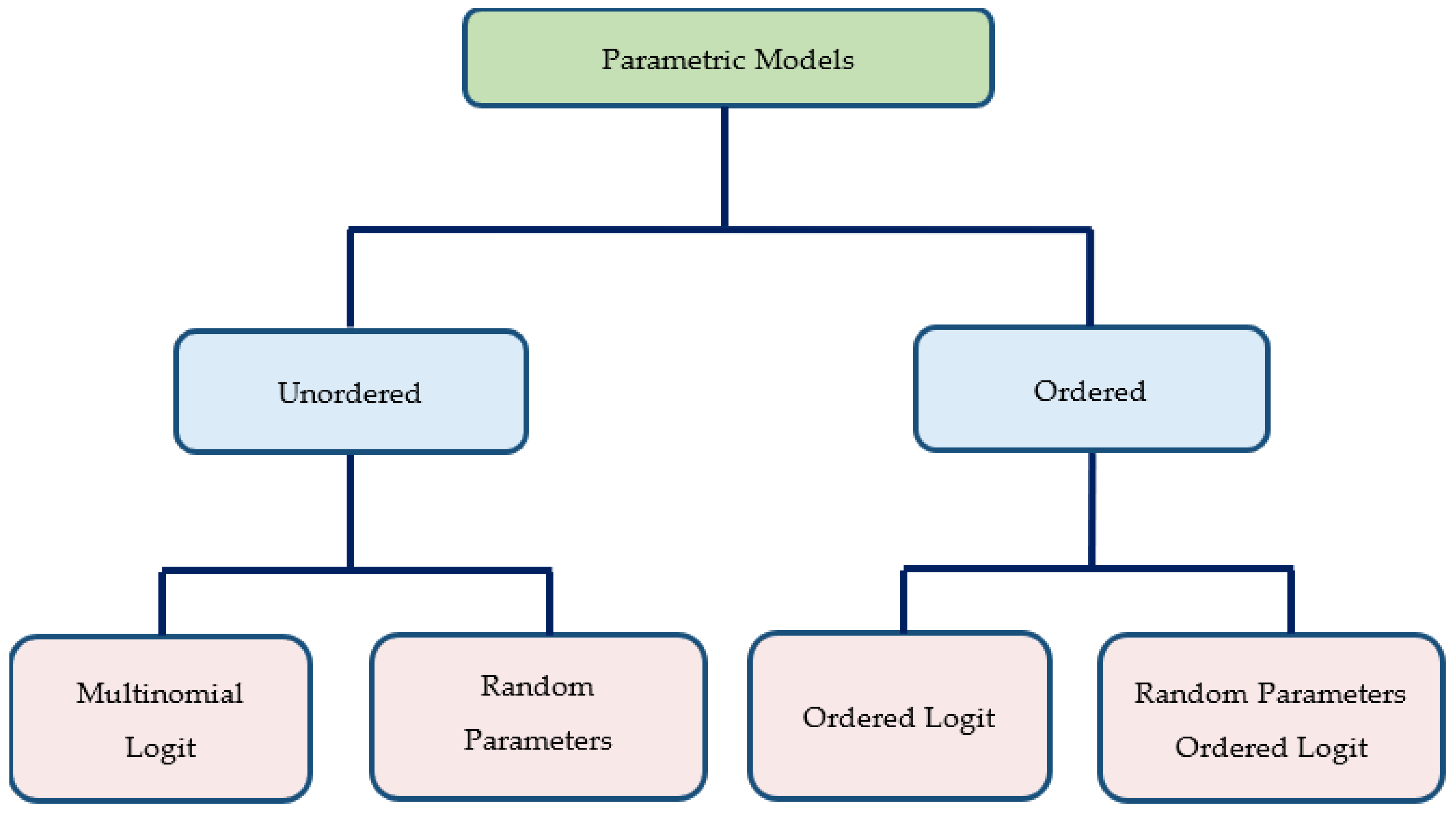
4.1. Parametric Models

4.1.1. General Issues

Econometric models, which are also referred to as “discrete choice models”, are widely used in crash severity analyses. These models use the theoretical utility (Uij), which, in the context of road safety applications, represents the propensity that a crash (i) will be recorded with a severity level (j), following the expression reported below [35]:
Uij = Vij + εij
where Vij is the systematic component; and εij is the disturbance term.
The crash severity, as a three-level variable, is very adaptable to econometric models with both unordered and ordered formulations. Indeed, each level of crash severity is linked to: (1) The increasing severity of the most seriously injured person that is involved in the crash; and to (2) The increasing costs in terms of the human, medical, and damage factors, which involve losses in terms of the life years and the quality of life. Thus, the crash severity has an ordinal nature, which could be addressed by performing the analysis with the ordered formulation. In this study, we used both unordered and ordered logit models. Furthermore, both unordered and ordered models were used in the standard formulation with fixed parameters, as well as in the formulation with random parameters (Figure 2). The random parameter models allow the effects of the independent variables to vary across different observations (i.e., the crashes in our study).
All of the models were estimated by maximum likelihood stepwise methods. The forward stepwise approach to choosing a model begins with a null model, and it adds terms sequentially until further additions do not improve the fit. At each stage, it selects the term that produces the greatest improvement in the fit [36,37].
For choosing the correct model, the likelihood ratio (LR) test is estimated as part of the random ordered/unordered model in order to determine the significance of the random formulation relative to the standard ordered/unordered logit model. The LR test compares the likelihood of the mixed model to the likelihood of the standard model:
LR   test = 2 log ( L MIXED L ST ) = 2 ( log L MIXED log L ST )
where L MIXED is the likelihood of the mixed model; and L ST is the likelihood of the fixed parameter model.
The likelihood ratio test statistic has an approximate χ2 distribution, with k (the number of predictors) degrees of freedom. If the LR   test p-value is less than 0.05, the random parameter logit model is superior to the standard model, with over 95% confidence. This indicates that the random parameter multinomial logit model provides a statistically superior fit relative to the traditional fixed parameter model [38].
Cross-validation was used to determine the generalizability and the overall utility of the prediction models.
All of the explanatory variables were transformed into dummy variables through a complete disjunctive decoding process. The predictors with multiple categories (k) were converted to a series of indicator variables (dummy variables) with k−1 variables, and the k-th dummy variable was not inserted into the model in order to avoid incurring the problem of perfect multicollinearity. All of the indicator variables were used to estimate the four logistic regression models and were tested for inclusion. Each indicator variable was assessed for its importance to the injury severity by using the z-test, with a significance level of 10%. All four models were developed using the STATA software.

4.1.2. Multinomial Logit Model

The crash severity analysis can be carried out by considering the three classes (slight injury, serious injury, and fatal crashes) as the possible discrete outcomes. In the general case of a multinomial logit model for the crash injury severity outcomes, the propensity of the crash (i) (i = 1, …, I) towards the severity category (j) (j = 1, …, J) is represented by the severity propensity function [14]:
U i j = V i j + ε i j = β j x i j + ε i j
where Vij is the systematic component;
  • ε i j is the disturbance term, which is assumed to be independently and identically distributed following the Type I generalized extreme value distribution (i.e., the Gumbel distribution), with the mean equal to zero and the variance equal to one, and the scale parameter is η [14,39];
  • x i j is a (K × 1) column vector of K exogenous attributes (geometric variables, environmental conditions, driver characteristics, etc.) that affects the pedestrian injury severity level (j); and
  • β j is a (K × 1) column vector of the estimable parameters for the crash severity category (j).
For a standard multinomial logit, the utility is linear in β , and then V i j = β j x i j . Each β j represents the estimated impact of the variable, x i j , on the response variable, y i . The standard multinomial logit formulation takes the following form:
P ( y i = j ) = P i ( j ) = e ( β j x i j + ε i j ) j = 1 J e ( β j x i j + ε i j )
In a standard multinomial logit formulation, the βs are assumed to be fixed across the observations, and the standard multinomial logit model is considered to be a fixed parameter model.
The factor exp(β) is the odds ratio (OR), and it indicates the relative amount by which the odds of the outcome increase (OR > 1) or decrease (OR < 1) when the value of the corresponding indicator variable is 1.

4.1.3. Random Parameter Multinomial Logit Model

The random parameter multinomial logit model, which is also known as the “mixed multinomial logit model”, is the generalized form of the multinomial logistic regression model, in which the coefficients of any of the variables are not limited to a fixed value but are allowed to vary across observations, or the analyst-specified groups of observations. This specification is the same as for the standard logit, except that, instead of being fixed, the β varies among the observations. The β coefficients are random and can be decomposed into their means and standard deviations [11]:
U i j = V i j + ε i j = β j x i j + ε i j ;   β j = B + β ˜ j
where Vij is the systematic component; εij is the disturbance term, which is assumed to be independently and identically distributed across the crash severity levels and the crashes; xij is a (K × 1) column vector of K exogenous attributes (geometric variables, environmental conditions, driver characteristics, etc.) that are specific to the crash (i) and that affect the pedestrian injury severity level (j); β j is a crash-specific (K × 1) column vector of the corresponding parameters that varies across the crashes on the basis of the unobserved crash-specific attributes; b are the means of the β′ random coefficients; and β ˜ j are the standard deviations of the β′ random coefficients.
Hence, the standard multinomial logit hypotheses are relaxed (i.e., the mixed logit does not exhibit independence from the irrelevant alternatives), and one or more parameters can be randomly distributed in the mixed model. Indeed, the presence of correlations between the unobserved characteristics of each observation violates the disturbance independence assumptions for the error terms, which leads to erroneous parameter estimates, whereas the random parameter model addresses the unobserved heterogeneity within the parameters that vary across the individual observations. If unobserved heterogeneity is allowed, then βj is a vector with a continuous density function, which means that the unconditional probability of an individual (i) experiencing the severity level (j) from the set of severity outcomes (J) is obtained by considering the integrals of the standard multinomial logit probabilities over the density of the parameters, and it can be expressed in the form [40]:
P i ( j ) = e β j x i j J e β j x i j f ( β | θ ) d β
where x i j is a (K × 1) column vector of K exogenous attributes (geometric variables, environmental conditions, driver characteristics, etc.) that are specific to the crash (i), and that affect the pedestrian injury severity level (j); β j is a crash-specific (K × 1) column vector of the corresponding parameters that varies across the crashes on the basis of the unobserved crash-specific attributes; f ( β | θ ) is the density function of the β coefficients; and θ is a vector of the parameters that describes the density function of the β coefficients in terms of the mean and the variance.
The random multinomial logit probability is expressed as the weighted average of the probability that is evaluated with the multinomial logit formula at different values of β, with the weights provided by the density function (f(β)). The standard multinomial logit is a special case of the mixed logit formulation because if β j = b for each observation, there is no crash-specific unobserved heterogeneity among the data, and the random parameter model coincides with the standard multinomial logit with fixed parameters (b), and f(β) = 1 for β j = b, while it is 0 for βj ≠ b.

4.1.4. Ordered Logit Model

The multinomial logit model disregards the ordered nature of the injury severity levels and treats them as independent alternatives; thus, the ordering information is lost [21]. The model is based on the cumulative probabilities of the response variables, and it is assumed that the logit of each cumulative probability is a linear function of the covariates, with regression coefficients that are constant across the response categories. In this case, the effects of the explanatory variables on the severity levels are assumed to be fixed across the observations. In other words, ordered logistic regression assumes that the coefficients that describe the relationship between the lowest versus all of the higher categories of the dependent variable (which is the crash severity in our study) are the same as those that describe the relationship between the next lowest category and all of the higher categories. This is also called the “proportional odds assumption”, “the parallel regression assumption”, or the “grouped continuous model” [41]. Assuming that the severity of a crash is an ordered discrete variable with j categories (slight, serious, and fatal), three levels are given meaningful numeric values, usually 0, 1, …, J (J is the upper limit). Slight, serious, and fatal might be labeled as “0”, “1”, and “2”, respectively, and the numerical values represent a ranking so that, for the crash severity, the “1” label is more severe than the “0” label in a qualitative sense, and the difference between the “2” and the “1” is not the same as for that between the “1” and the “0”. In this case, although the numerical outcomes are merely the labels of the non-quantitative outcomes, the analysis will nonetheless have a regression-style motivation [42]. The severity propensity function is assumed as it is reported in Equation (7), and the ordinal response ( y i ) can be expressed as:
y i = { 0   if U i μ 1 j   if μ j 1 < U i μ j J   if μ J 1 < U i +
where μj represents the upper threshold for the injury severity (J); μj−1 represents the lower threshold for the injury severity (J); and μj and μj−1 are the values of the cutoff, or the cut-points.
The cumulative probability can be written as [41]:
P i ( j ) = e ( β j x i j + ε i j μ j ) 1 + e ( β j x i j + ε i j μ j ) ,   j = 1 , 2 , , J 1

4.1.5. Random Parameter Ordered Logit Model

The random parameter ordered logit model allows the thresholds in the ordered logit model to vary on the basis of both the observed, as well as the unobserved, characteristics. It also accommodates the unobserved heterogeneity in the effects of the exogenous variables on the injury propensity and on the threshold values through a suitable specification of the thresholds that relaxes the restriction of identical thresholds [21]. As for the mixed multinomial logit model, Equation (10) determines the probability that the crash (i) will result in the injury-severity level (j). Hence, both the βs and the threshold (μ) can systematically vary across crashes because of the observed and unobserved factors: in an ordered random parameter logit model, the thresholds also consist of a systematic component and unobserved disturbance error terms, which thus allows for unobserved variability and randomness in the thresholds, as is expressed by the formula below:
μ i j = V j + τ i j
where V j is a systematic component; and τ i j is the unobserved disturbance error term.
Finally, the likelihood function for the individual (i) represents the probability of the injury severity that will be experienced by that individual, and it can be evaluated as:
P i ( j ) = e ( β j x i j + ε i j μ j ) 1 + e ( β j x i j + ε i j μ j ) f ( β | θ ) d β   j = 1 , 2 , , J 1
Therefore, in order to account for these circumstances, a random parameter ordered logit model was developed to capture the unobserved heterogeneity, which is achieved by adding a randomly distributed error term.

4.2. Non-Parametric Models

Five popular non-parametric algorithms, namely, association rules, classification trees, random forests, artificial neural networks, and support vector machines, were used to predict the injury severities of the pedestrian crashes. As data-driven and non-parametric methods, the machine learning algorithms do not require any a priori assumptions about the relationships between the variables.

4.2.1. Association Rules

As a descriptive–analytic methodology, the association rules are used for extracting knowledge from large datasets by generating rules that have the form: A→B. Each rule contains at least one pattern, which is called the “antecedent” (A), as well as a “consequent” (B). In our study, the latter consists of the fatal or serious injury severities. The a priori algorithm (which was introduced by Agrawal et al. [43]) generates rules by using simple and repetitive steps, and by examining all of the candidate item-sets in order to find the frequent item-sets, until no new ones can be produced. All of the valid rules satisfy the support, confidence, and lift thresholds, where the support is the percentage of the entire dataset that is covered by the rule (Equation (11)), the confidence measures the reliability of the inference of the rule (Equation (12)), and the lift is a measure of the statistical interdependence of the rule (Equation (13)):
S   ( A B ) = # ( A B ) N ;   S ( A ) = # ( A ) N ;   S   ( B ) = # ( B ) N ;
Confidence = S ( A B ) S ( A )
Lift = S ( A B ) ( S ( A ) × S ( B ) )
where S(A→B) is the support of the association rule; S(A) is the support of the antecedent; S(B) is the support of the consequent; #(A→B) is the number of crashes, where both Conditions A and B occur; #(A) is the number of crashes with A as the antecedent; #(B) is the number of crashes with B as the consequent; and N is the total number of crashes in the dataset.
A rule with a single antecedent and a single consequent is defined as a “two-item rule”; similarly, a rule with two antecedents and a single consequent is defined as a “three-item rule”. Each rule with n + 1 items is validated by verifying that each variable produces a lift increase (LIC). The LIC ensures that each additional item in the rules leads to an increase in terms of the lift.
The rules with only one item in the antecedent are used as a starting point, and the rules with more items are selected over simpler ones by verifying that each variable produces a lift increase (LIC) that is not smaller than 1.05 [44]. The LIC ensures that each additional item in the rules leads to an increase in terms of the lift. The LIC is calculated as follows:
LIC = Lift A n Lift A n 1
where An−1 is the antecedent of the rule with n−1 items; and An is the antecedent of the rule with n items.
The threshold values of the support (S), the confidence (C), and the lift (L) were set as follows: S ≥ 0.1%; C ≥ 4.0%; L ≥ 1.2; and LIC ≥ 1.05. The association rules were performed in the R-CRAN software environment using the package, “arules”.

4.2.2. Classification Trees

A classification tree is a nonlinear tool and an oriented graph, where the root node is divided into leaf nodes by an explanatory variable that is also called the “splitter”. All of the independent variables are candidates for the splits at each internal node of the tree. However, only the predictor that provides the best partition is chosen. In our study, we developed the CART algorithm, which was introduced by Breiman et al. [45], and the impurity at each node was assessed by the Gini reduction criterion (the higher the value of the Gini index, the higher the homogeneity of the node that is due to the split), which can be calculated as follows:
i Y ( t ) = 1 j p ( j | t ) 2
where P(j|t) is the proportion of the observations in the node (t) that belong to the class (j).
If a node is “pure”, all of the observations in the node belong to one class, and the impurity of that node is zero.
The total impurity of any tree (T) is defined as follows:
i Y ( T ) = t T ˜ i Y ( t ) p ( t )
where iY(t) is the impurity of the node (t); p(t) = N(t)/N is the weight of the node (t); N(t) is the number of observations that fall in the node (t); N is the total number of observations; and T ˜ is the set of terminal nodes of the tree (T).
By definition, the terminal nodes present low degrees of impurity compared with the root node.
The total impurity of the tree is reduced by finding, at each node of the tree, the best partition of the observations into disjoint classes, which are externally heterogeneous and internally homogeneous.
The choice of the best classification rule was made through the V-fold cross-validation estimate. The initial set (S) is randomly divided into a V > 2-fold (Sv for v = 1, 2 …, V). The corresponding estimate of the error rate is given by:
E R v CART = i = 1 N v ( Y ^ CART ( X i ) Y i ) N v
where Y ^ CART ( X i ) is the predicted class for the ith observation; X i is the vector of the descriptors of the ith observation; Y i is the class label of the ith observation; and N v is the numerosity of the set (Sv).
The estimate of the error rate, which is based on cross-validation (ER), is obtained by combining the individual estimates for all the possible subsets (Sv).
ER = v = 1 V E R v CART V
The tree growing was stopped on the basis of two criteria: (1) If the reduction in the Gini measures was less than a prespecified minimum fixed value that was equal to 0.0001 (default value); and (2) If the maximum number of levels of the tree were equal to 4. These parameters were chosen to minimize the error rate.
The class assigned to each node was selected according to the greatest value of the posterior classification ratio (PCR) that was evaluated for that node. The PCR compares the classification of the terminal nodes of the tree with the classification of the root node, and it is calculated as follows [24]:
P C R ( j | t ) = p ( j | t ) p ( j | t root )
where p(j|t) is the proportion of the observations in the node (t) that belong to the class (j); and troot is the root node of the tree.
One of the outputs that is provided by the CART technique is the variable importance, which defines the variable’s ability to influence the model. The relative importance of the variable (VI) (Xj) is calculated as follows:
V I = t = 1 T N ( t ) N Δ i Y ( t , s )
where VI represents the relative importance of the variable (Xj); ΔiY(t,s) is the reduction in the Gini index that is obtained by splitting the variable (Xj) at the node (t); N is the total number of observations; and T is the number of nodes in the tree.
The classification trees were carried out with SPSS software.

4.2.3. Random Forests

Classification trees, despite their advantages, have sometimes been found to generate unstable predictions given certain perturbations; thus, in order to improve the stability, Breiman [46] proposed the RF method. RFs are an ensemble of B trees {T1(X), …, TB(X)}, where Xi = {xi1, …, xip} is a p-dimensional vector of the descriptors or properties that are associated with the ith crash. The ensemble produces B outputs {Ŷ1 = T1(X), …, ŶB = TB(X)}, where Ŷb, b = 1, …, B, is the prediction for a crash by the bth tree. The outputs of all of the trees are aggregated to produce one final prediction: Ŷ. For classification problems, Ŷ is the class that is predicted by the majority of the trees.
Given the data on a set of n crashes, D = {(X1, Y1), …, (Xn, Yn)}, where Xi is a vector of the descriptors, and Yi is the corresponding class label for the ith crash, with i = 1, …, n. The algorithm proceeds as follows:
  • A bootstrap sample, which creates a random sample with a replacement from the original sample, with the sample size (Nt) replicated B times.
  • For each bootstrap sample, the growing of a tree uses the CART algorithm, and chooses, at each node, the best split among a randomly selected subset of descriptors;
  • Repeat the above steps until B trees are generated.
However, it has been shown that there is a potential overestimate of the true prediction error, depending on the choices of the random forest hyperparameters, such as the number of trees (B), and the number of descriptors. To reduce the true prediction error, the out-of-bag estimate of the error rate (EROOB) was estimated by varying the B and the number of descriptors:
ER OOB = i = 1 N ( Y ^ OOB ( X i ) Y i ) N
where Y ^ OOB ( X i ) is the predicted class for the ith crash; X i is the vector of the descriptors of the ith crash; Y i is the class label of the ith crash; and N is the total number of crashes.
The values of the number of trees and the number of descriptors were chosen so that the EROOB tends to stabilize around the minimum value.
The variable importance measure for the variable, x j , ( V I ( x j ) ), is computed as the sum of the importances over all of the trees in the forest:
V I ( x j ) = t = 1 ntrees V I t ( x j ) ntrees
where V i t ( x j ) is the variable importance of the tth tree that is calculated using Equation (20); and ntrees is the number of trees.
The RF was performed in the R-CRAN software environment using the packages, “randomForest”, and “randomForestSRC”.

4.2.4. Artificial Neural Networks

As is the classification tree and the RF, the ANN is also an oriented graph that is inspired by a biological neural network. Similar to the structure of the human brain, the ANN models consist of neurons in complex and nonlinear forms. The ANN models work by creating a nonlinear relationship between the dependent and independent variables, depending on a set of experimental data. The neurons are connected to each other by weighted links. ANNs consist of a layer of input nodes and a layer of output nodes that are connected by one or more layers of hidden nodes. The input-layer nodes pass information to the hidden-layer nodes by firing the activation functions, and the hidden-layer nodes fire, or remain dormant, depending on the evidence that is presented. The hidden layers apply weighting functions to the evidence, and, when the value of a particular node or set of nodes in the hidden layer reaches a certain threshold, the value is passed to one or more nodes in the output layer.
The technique creates a feed-forward multilayer perceptron ANN, which consists of multiple nodes (or neurons) that are organized into three or more layers, with a backpropagation learning process to minimize the classification errors. In our study, a three-layer network was implemented, as previous studies suggest that ANNs with singular hidden layers are less likely to be trapped at a local minimum [47,48]. Thus, the information flows from the input layer, passes through the hidden layer, and then flows to the output layer to produce a classification. The hidden layer has 1 + p = 1 p k p neurons (consider a dataset that contains P independent variables that are classified on the kp potential risk factors that have effects on the crash severity), and each risk factor is represented by a node, while another constant node is included, which represents the bias. The output layer has three neurons, which accord with the three severity levels in the study.
The neurons of the input layer transfer information to the hidden layer through the hyperbolic tangent activation function, and from the hidden layer to the output layer through the softmax function.
z = softmax [ j = 1 J w j ( 2 ) tanh ( p = 1 p w j , p ( 1 ) k p ) ]
where J is the number of neurons in the hidden layer; w j , p ( 1 ) is the connection weight between the hidden node (j, j = 1, … J) and the input node (p, p = 1, …, P); kp are the factors; and w j ( 2 ) is the weight of the connection between the output node (z) and the hidden node (j).
In the output layer, Z = 3 nodes expresses the severity outcomes that are predicted by the ANN, and yi is the ith observed response in the dataset. If, for the ith crash, yi = z, then z = 1, while z = 0 if otherwise.
The connection weights were estimated by using a backpropagation learning process to minimize the classification errors. Standard backpropagation is a gradient descent algorithm in which the network weights are moved along the negative of the gradient of the performance function. The combination of weights that minimize the error function is considered to be a solution to the learning problem. The backpropagation algorithm proceeds as follows:
  • The backpropagation algorithm starts with random weights, and the goal is to adjust them to reduce this error until the ANN learns the training data;
  • If the expected output is not obtained, backward propagation begins. The difference between the actual and the expected outputs is calculated recursively and step by step, and the error is returned through the original link access;
  • The weight and the value of each neuron are then modified and are transmitted successively to the input layer, and the forward multilayer perceptron restarts.
These two processes (forward multilayer perceptron and backpropagation error) are repeated so that the error gradually decreases. The goal is to minimize the error by adjusting the weights so that the optimum weights are obtained after the error backpropagation.
The gradient (G) of a weighting to the error, the total error (E), and the total mean square errors ( e p ) are defined as:
G = E w
E = e p
e p = 1 2 k 1 m ( y k p y ¯ k p ) 2
where w is one of the network weightings (wpl, wjp, wkj); y k p is the actual output; and y ¯ k p is the expected output.
The adjustment of the weight is calculated as:
Δ w new = η G + α Δ w old
where Δ w new is the present adjustment for the weighting or for the threshold; Δ w old is the immediate past value of its counterpart; α is a dynamic coefficient, and it takes a value in the range of between 0 and 1; and G is the gradient of a weighting to the error.
This procedure was applied to the categorical data after transforming the categorical variables into dummy variables through a complete disjunctive decoding process. The predictors with multiple categories (k) were converted into a series of indicator variables (dummy variables) with k variables.
Moreover, the k-fold cross-validation procedure was used in each modeling phase of the ANN.
The importance of a specific explanatory variable is determined by identifying all of the weighted connections between the nodes of interest. All of the weights that connect the specific input node, which passes through the hidden layer to the specific response variable, are identified. This is repeated for all of the other explanatory variables, until all of the weights that are specific to each input variable are determined.
The ANN was performed with the SPSS software.

4.2.5. Support Vector Machines

A SVM, which was developed by Cortes and Vapnik [49], is used to develop an optimal separating hyperplane to categorize the observations into several groups, while maximizing the margin between the decision boundaries and minimizing the empirical error. The predictors are defined as the vectors (Xi = {xi1, …, xip}), where p represents the full set of crash-related variables, and the outcome is defined as yk, which represents the injury severity levels of the crashes. Hence, the plane constitutes the decision boundaries, and the hyperplane is a p−1 dimensional plane. The decision boundaries may or may not be linear, depending on the pre-set kernel function. The radial basis function (RBF) is the most commonly used for crash severity analyses since it is capable of capturing the nonlinearity relationships between the crash severity and the explanatory variables [50]:
K (Xi, Xj) = exp (−ϒ |Xi − Xj|2), ϒ > 0
where Xi and Xj are the vectors of the explanatory variables for the ith and the jth crashes; |Xi−Xj|2 is the Euclidean distance between the two crashes, Xi and Xj; and ϒ = 1/σ2, where σ2 is the variance of the samples selected by the model as support vectors.
The development of the SVM model also depends on the penalty parameter (C) of the error term. It controls the trade-off between smooth decision boundaries, and the correct classification of the points, and it is calculated as follows:
ER SVW = i = 1 N ( Y ^ SVM ( X i ) Y i ) N
where Y ^ SVM ( X i ) is the predicted class for the ith crash; X i is the vector of the descriptors of the ith crash; Y i is the lass label of the ith crash; and N is the total number of crashes.
To determine the separability of the optimal hyperplane, a grid search was used for the joint optimization of the C and γ parameters and for the feature selection. This approach methodically builds and evaluates a model for each combination of algorithm parameters (γ and C) that are specified in a grid. For each model, the classification error was used as a performance measure. The combination of the hyperparameters with the lower classification error was chosen in order to develop the optimal hyperplane.
To effectively combine these parameters, and to avoid overfitting, the cross-validation method was used for each developed model, which provided information about how well the SVM generalizes, specifically in terms of the range of expected errors.
The variables that contribute to the separability of the optimal hyperplane provide an indication of the relative importances of the variables to the separation.
The SVM was performed in the R-CRAN software environment using the packages, “caret” and “e1071”.

4.3. Dealing with Imbalanced Data

The study data are characterized by imbalanced classes, with order ratios of 2:100 for the fatal crashes, and of 25:100 for the serious injury crashes. The issues that are relative to the classification performance with imbalanced data have been highlighted in previous studies (e.g., [30,31,33,51]).
To take into account the skewed distribution of the classes, different weights were given to both the majority and minority classes. The difference in the weights influenced the classification of the classes during the learning phase. The whole purpose is to penalize the misclassification that is made by the minority class by setting a higher class weight and, at the same time, reducing the weight for the majority class. The weight was assigned so that the response variable was equally distributed among the categories. The class weights are inversely proportional to their respective frequencies [52,53,54]. Each weight can be assessed as follows:
W k = N crashes n c × N k
where k is the number of the crash severity level, with 1 = slight injury; 2 = serious injury; and 3 = fatal; wk is the weight that is assigned to the respective level of severity (k); Ncrashes is the total number of crashes in the dataset; nc = 3, which is equal to the number of crash severity levels that are considered in the study; and Nk is the number of crashes with a severity level (k).

4.4. Comparison among the Models

A classifier aims to minimize the false positive rates (which represent Type I errors) and the false negative rates (which represent Type II errors), which maximizes the true negative and positive rates. Among the common performance metrics that are used to evaluate the classification performance, the accuracy and the error rate are the most widely used. However, when the distribution of the response variable is extremely imbalanced, the accuracy has certain limitations. The error rate suffers from similar drawbacks. First, it is easy to obtain high accuracies (or low error rates) under highly imbalanced problems. Secondly, these classifiers assume that the errors are of equal value, which is not true for the imbalanced data, where misclassifying the instances of the minority classes (fatal and serious injury crashes) is generally much costlier than misclassifying the instances of the majority class (slight injury crashes) [55,56]. Moreover, the correct classification of the factors that contribute to fatal and serious injury crashes is a far cry from the correct identification of the factors that contribute to slight injury crashes.
Hence, we chose to assess the multiparameter indicators, namely, the F-measure, the G-mean, and the area under the curve (AUC), in order to evaluate the performances of the implemented models in a single measure.
The performance measures are expressed as follows [33]:
Acc   =   TN TN + FP   =   specificity
where Acc is the true negative rate, which is also known as the “specificity”; TN is the number of true negatives; and FP is the number of false positives.
Acc +   =   TP TP + FN   =   Recall   =   sensitivity
where Acc + is the true positive rate, which is also known as the “recall”, or the “sensitivity”; TP is the number of true positives; and FN is the number of false negatives.
G - mean   =   ( Acc   ×   Acc + ) 1 2
Precision = TP TP + FP
F - measure = ( 1 + β 2 ) × Precision × Recall Precision + Recall
where β is a coefficient for adjusting the relative importance of the precision and recall, which is set at a value that is equal to 1.
The G-mean combines the performances of the positive and negative classes, whereas the F-measure combines the cases that are correctly classified with the Type I and Type II errors. Indeed, when the errors increase, the F-measure decreases. The F-measure is also the weighted harmonic mean of the precision and recall (which are both referred to as the “minority class”), and a high F-measure usually indicates the model’s good overall performance. The AUC is the area under the receiving operating curve (ROC), and it is a widely used graphical plot that illustrates the ability of a classifier that is assessed by plotting the true positive rate (TPR) (which is also known as the “sensitivity”) on the vertical axis against the false positive rate (FPR) (which is also known as the “specificity”) on the horizontal axis at various threshold settings. When the ROC curve is created, the AUC can be assessed. The AUC represents the probability that the classifier correctly identifies an observation that is randomly selected among the positive cases. An AUC value varies between 0 and 1. An AUC greater than 0.60 is considered satisfactory [57].
Once the performance metrics for each class are evaluated, the final values are the weighted mean, in which the relative frequencies of the classes on the data are their weights [58].

5. Results

5.1. Parametric Models

All the explanatory variables that are reported in the appendix section (Table A1, Table A2, Table A3, Table A4, Table A5 and Table A6) were tested for inclusion in the econometric models. The estimation results are reported in Table 2, Table 3, Table 4 and Table 5. The variable indicators that are not statistically significant at the 0.10 level of significance, either for the fatal crashes or for the serious injury crashes, were removed from the tables.

5.1.1. Multinomial Logit Model

There were 20 statistically significant explanatory variables, and 41 significant indicator variables that were associated with these categorical variables (Table 2). The model’s McFadden Pseudo R2 is equal to 0.16. The most influential variable is the pedestrian age. Compared to young pedestrians (35–44 years), the elderly pedestrians (aged 75 years or more) had increased probabilities of fatal crashes, with an OR of 13.17. Another significant indicator is speed limits ≥ 50 mph., for which the indicator exhibited an OR equal to 9.27.

5.1.2. Random Parameter Multinomial Logit Model

The results for both the fixed and random variables are reported in Table 3. The log-likelihood at zero (−48,217) and at convergence (−39,565) give a McFadden R2 of 0.18, which is a good result. It is also the highest value that is exhibited among the parametric models that were performed in this study. The goodness-of-fit results and the LR test results show that the random model provides a significant improvement compared to the fixed parameter model. The χ2 of the LR test is 1808.11, with 3 degrees of freedom, and a p-value < 0.001, which shows that the random parameter multinomial logit model is superior to the standard multinomial logit model, with over 99.9% confidence. Three of the indicator variables show normally distributed random parameters, with statistically significant standard deviations, which indicates a significant unobserved heterogeneity in the data (Table 3). These variables are: (1) Going-ahead vehicle maneuvers (fatal); (2) Roundabouts (fatal); and (3) A pedestrian age greater or equal to 75 (serious injury). In the prediction of fatal severity, the indicator variable, “roundabout”, shows a normal distribution, with a mean of −2.477, and a standard deviation of 2.583. This means that, for 83.1% of the crashes at roundabouts, the probability of the fatal outcome decreased, while, for 16.9% of the observations, the probability of a fatal outcome increased. Similarly, the indicator variable, “going-ahead maneuver”, shows a normal distribution, with a mean of 0.831, and a standard deviation of 0.997. This means that, for 79.8% of the observations with vehicles that maneuvered going ahead, the probability of a fatal outcome increased, while, for 20.2% of the observations, the probability of a fatal outcome decreased. In the prediction of severe injury, the indicator variable, “pedestrian age ≥ 75”, shows a normal distribution, with a mean of 0.297, and a standard deviation of 3.852. This means that, for 53.1% of the observations with pedestrian ages ≥ 75, the probability of severe injury increased, while, for 46.9% of the observations, the probability of severe injury decreased. The fixed coefficients of the random parameter multinomial logit were similar in sign and magnitude to the standard multinomial model.

5.1.3. Ordered Logit Model

The ordered logit model was carried out to capture the ordinal nature of the response variable. A positive (or negative) parameter implied the likelihood (or unlikelihood) of a severe injury, with an increasing value of the explanatory variable, and a reduction in the likelihood of a slight injury. There were 18 statistically significant explanatory variables, and 35 significant indicator variables that were associated with these categorical variables (Table 4). The model’s McFadden Pseudo R2 is equal to 0.15, which is the lowest value of fit that is exhibited by the parametric models in the study. Consistent with the unordered models, the most influential variable was the “pedestrian age”, which is also the case in the ordered logit model.

5.1.4. Random Parameter Ordered Logit Model

The results for both the fixed and the random variables are reported in Table 5. The goodness-of-fit results and the LR test results show that the random model provides a significant improvement compared to the fixed parameter model. The χ2 of the LR test is 1832.61, with 1 degree of freedom, and a p-value < 0.001, which shows that the random parameter ordered logit model is superior to the standard ordered logit model, with over 99.9% confidence.
One indicator variable showed normally distributed random parameters, with statistically significant standard deviation, which indicates significant unobserved heterogeneity in the data (Table 5). This variable is the “pedestrian age ≥ 75”. In the prediction of both the fatal and severe injury severities, the indicator variable, “pedestrian age ≥ 75”, showed a normal distribution, with a mean of 0.258, and a standard deviation of 0.580. This means that, for 67.8% of the observations with pedestrian ages ≥ 75, the probability of the most severe injury increased, while, for 32.8% of the observations, the probability decreased. Similar to the unordered models, the fixed coefficients of the random parameter ordered logit model were similar in sign and magnitude to the standard ordinal model.

5.2. Non-Parametric Models

5.2.1. Association Rules

The a priori algorithm generated 254 rules with the fatal crash as the consequent, and 475 rules with the serious injury crash as the consequent. Furthermore, the extracted rules exhibited, at most, three items as antecedents. Among the rules with the fatal crash as the consequent, 97 rules include the “pedestrian age ≥ 75” as the first antecedent, 53 rules include “vehicle engine capacities (CCs) not smaller than 3000+”, 33 rules include “rural area”, 26 rules include “vehicle skidding and overturning”, and 15 include “lighting equal to darkness—no lighting”. Table 6 contains a selection of the high-lift rules with the fatal crash as the consequent. The pedestrian age also generated a considerable number of significant rules for the serious injury crash as the consequent. Out of the 475 rules with the serious injury crash as the consequent, 237 rules exhibited the “pedestrian age” as the first item, which were followed by 74 rules with the “number of pedestrians involved in a crash”, and “driver age < 25”, with 33 rules.
Table 7 contains the strongest rules that predict serious crashes.

5.2.2. Classification Tree

The classification tree is reported in Figure 3. The tool generated 15 terminal nodes, 10 of which predicted fatal crashes, 3 of which predicted serious crashes, and 2 of which predicted slight injury crashes. The posterior classification ratio (PCR) was assessed for all the nodes, but it was reported only for the terminal nodes in order to understand how representative each terminal node is in relation to the predicted class. Node 17 and Node 19 exhibited very high PCRs (13.10 and 17.45, respectively), which implies the robustness of both terminal nodes for the “fatal” classification.
The analysis of the variable importance (Figure 4) identified four variables as having the most influence on the classification accuracy of the pedestrian crash severity: (1) The speed limit; (2) The pedestrian age; (3) The lighting; and (4) The area.

5.2.3. Random Forests

Initially, a RF was implemented, which generated 500 trees. However, the hyperparameter-tuning process provided the RF optimal number of trees as 42. Then, the RF was performed again, and the most important predictors that were associated with the fatal and severe pedestrian crashes were determined. The importance of each explanatory variable is assessed by observing how the prediction error increases when the data that are not in the bootstrap sample (what Breiman calls, “OOB data”) are permuted for that variable, while all of the others are left unchanged. The score rankings of the explanatory variable importances are provided in Figure 5 below. According to the Gini impurity, four variables were identified as having the most influence on the classification process of fatal pedestrian crashes: the vehicle maneuver, the pedestrian age, the vehicle’s first point of impact, and the driver gender, whereas, as far as serious crashes are concerned, the RF highlights the severe impact on the pedestrian crash severity of factors such as the vehicle maneuver and the driver gender, and it also identifies as critical the presence of “vehicle towing and articulation”, and of the vehicle type.

5.2.4. Artificial Neural Networks

The ANN tool generated a graph that contains 26 factors and 132 neurons in the input layer (excluding the bias unit), and 13 hidden nodes in the hidden layer, whereas the output layer had three neurons that represented the three injury levels.
The input and hidden layers were linked through the hyperbolic tangent transfer functions, whereas the transfer function between the hidden layer and the output layer was the softmax function. A total of 13 factors exhibited high impacts on the pedestrian crash severity (Figure 6), with normalized importances greater than 50%: the driver and pedestrian ages; the vehicle engine; the lighting; the vehicles’ first point of impact; the speed limit; the vehicle maneuver; the vehicle type; the area; the first road class; the weather; the junction detail; and the pedestrian-crossing physical facilities.

5.2.5. Support Vector Machine Model

The SVM model was performed with the RBF kernel function. The model returned 19,909 support vectors, which defined the complex hyperplane. The SVM model provides the visualization of the most relevant features through nonlinear kernels that are necessary to carrying out the classification process. The importance of the predictors that were exhibited by the tool (Figure 7) was used to compare the SVM output with the outputs of the other non-parametric algorithms that were implemented in the study. The SVM model identified four predictors, which mostly contributed to the correct classification of the pedestrian crash severity: the first road class; the pedestrian age; the pedestrian-crossing physical facilities; and the junction detail.

5.3. Model Comparisons

In this section, the comparisons among the nine implemented methods are provided, with an analysis of both the significant explanatory variables that affect the crash severity (qualitative evaluation), as well as of the model performances (quantitative evaluation).

5.3.1. Significant Explanatory Variables and Effects on Crash Severity

The results of the parametric and non-parametric models highlight that the non-parametric models tend to uncover more hidden correlations among the data than the parametric models.
A total of 19 variables are significant in both the parametric and the non-parametric models, and 1 variable is identified only by the first group of models, whereas 7 variables turn out to be important in the non-parametric classification process.
The same variables are significant with reference to both fatal as well as serious injuries, except for the vehicle propulsion code (which is significant only for the fatal severity) and the number of pedestrians involved (which is significant only for serious injuries). The “pedestrian-crossing human control” is the variable that is significant only in the econometric model, while the variables that are significant only in the machine learning algorithms are the “driver home area”; the driver journey purpose; the number of pedestrians involved; the vehicle’s first point of impact; the vehicle engine capacity; the weather; and the junction control. In the appendix, we summarize the significant explanatory variables that are associated with an increase in the crash severity. Table A7 contains the variables that associated with an increase in the fatal crash probability, while Table A8 contains the variables that are associated with an increase in the serious crash probability.

Pedestrian Characteristics

All of the methods found a correlation between the pedestrian age and gender, with both fatal and serious crashes. The results indicate that elderly pedestrians (at least 65 years old) are very exposed to the most serious crashes, even though the parametric models and the association rules highlight “pedestrians ≥ 75” as the most vulnerable once in a crash. The pedestrian age was also among the strongest predictors in the classification tree, the RF, the ANN, and the SVM variable importance lists, with over a 50% influence on the classification. As far as the pedestrian gender is concerned, only the parametric methods and the association rules found greater propensities of male pedestrians towards the most serious crashes.

Driver Characteristics

The driver gender was among one of the most important predictors that were identified by the RF for fatal crashes. The result was consistent with the association rule results and all of the parametric models, which identified males as the drivers that are most likely to be involved in fatal and serious crashes. Very young drivers (age ≤ 24 years) also showed great propensities towards the most severe crashes. The relation was identified by all the parametric models (both in fatal and serious crashes) and the association rules (in serious crashes). Furthermore, the driver age was the most important predictor among the variable importances that was exhibited by the ANN. Furthermore, only the association rules identified aspects related to the driver’s purpose of the journey and the driver’s home area. “Journey as part of work” and “commuting to/from work” were considered critical, both for fatal and serious pedestrian crashes.

Vehicle Characteristics

All of the parametric models and the association rules identified a significant effect of old vehicles (vehicle age ≥ 15 years) on the most serious crashes. The parametric models provide positive coefficients for both fatal and serious crashes, and the results are consistent with the association rules. The vehicle type involved in a pedestrian crash affects the pedestrian outcome. Specifically, a pedestrian struck by a truck has a higher injury risk. The results were highlighted by all of the methods. A further risk for pedestrian safety was the presence of articulated vehicles, and the factor was identified by the association rules as the strongest two-item rule for fatal crashes. The relation was confirmed by the parametric models and the RF. By the parametric models, heavy oil vehicles were also identified as affecting the crash severity, with positive coefficients, whereas hybrid vehicles exhibited reductions in the crash severity. However, the association rules also found an association of fatal crashes to vehicles with petrol propulsion. Furthermore, the ANN tool identified the vehicle engine capacity as affecting the pedestrian crash severity.

Roadway Characteristics

The parametric models identified the increase in the speed limit as a contributory factor towards increasing the crash severity. The speed limit was also the first split for the classification tree growth, with higher speed limits associated with fatal crashes. The association rules identified high-lift rules with the fatal severity as the consequent, and a speed limit ≥ 50 mph as the antecedent. The speed limit was also identified as one of the most important predictors by the ANN, with 70% importance. All of the models also pointed to the “first road class equal to A” and “rural areas” as patterns that influence the crash severity, and this may be due to their correlations with higher speed limits.

Junction Characteristics

Pelican, puffin, toucan, or similar nonjunction pedestrian light crossings were found to increase the pedestrian crash severity. As far the junction detail is concerned, the econometric models did not provide the factors that influence the severity levels. By contrast, the association rules found that T or staggered junctions, or give-way/uncontrolled intersections, affected fatal and serious crashes in the presence of elderly pedestrians and van vehicles.

Environmental Characteristics

The day of the week, the lighting, the pavement, and the weather at the time of the crash were significant variables. The results indicate that the weekend is a predictor of fatal and serious crashes in both the parametric and the non-parametric models. In particular, this result of the parametric models was confirmed by the association rules. Darkness that is due to the absence of lights, or to inadequate lighting, increases the likelihood of the most severe crashes. The pavement condition affects the crash severity, particularly when it is wet or damp. The parametric models and the association rules found consistent results. The weather conditions were only highlighted by the ANN, which associates 60% of the importance in the classification to the weather variable. However, neither the other non-parametric models nor the parametric models confirm this result.

Crash Characteristics

The number of vehicles involved in the crash played a pivotal role. All of the parametric models show an increase in the probability of both fatal and serious injuries with multivehicle crashes. The relation was also captured by the association rules (Rule 34, L = 5.00). A frontal vehicle impact was identified as critical by the association rules, and this was confirmed by the RF and ANN tools. The association rules further identified the association of the number of pedestrians involved in the crash with serious crashes, and the association was identified only by the association rules. The generated two-item rule is the strongest one for serious crashes.

5.3.2. Measures of Performance

The performances of the models were evaluated by the F-measure, the G-mean, and the AUC. The results are shown in Table 8 and Table 9. Table 8 reports the performance measures that were exhibited by the parametric models, both in their standard formulations, without applying any treatment to the imbalanced data, as well as in their weighted formulations, after the implementation of the weighted approach that is presented in Section 4.3. Table 9 reports the performance measures of the non-parametric algorithms in the standard and weighted formulations. After the implementation of the weighted approach, all of the methods exhibited a relevant improvement in the classification performances, except for the association rules, where the weighted formulation did not significantly affect the model’s performances. The comparison among the different models shows several interesting results.
As far as the parametric models are concerned, the multinomial logit (fixed parameters) and random parameter multinomial logit (mixed parameters) models exhibited better classification performances, compared with their ordered versions (ordered logit and random parameter ordered logit models). Furthermore, the ordered logit model showed a poor ability in correctly classifying fatal crashes, even after the weighting procedure. Our results are consistent with previous studies [12,18]. The random parameter models (both the random parameter multinomial logit model and the random parameter ordered logit model) relax the restrictive assumption of the fixed model structure, which allows the exogenous variables to vary over the threshold parameters and to outperform their standard fixed parameter variants (multinomial logit and ordered logit models). Finally, our results found out that, among all the parametric models that were implemented in the study, the random parameter multinomial logit model has the best predictive performances (on average, an F-measure equal to 0.42, a G-mean equal to 0.59, and an AUC equal to 0.70), and it provides additional insights into the distribution of the parameters (by capturing attributes with mixed effects).
As far as the non-parametric tools are concerned, the SVM outperformed the other methods, and it is the best-fit model, according to the F-measure, the G-mean, and the AUC, both for fatal and serious injury crashes. The model reached an accuracy in both the correct positive and negative case classifications that is equal to 95%. The RF exhibited performances that were only slightly worse to the SVM, with accuracies in both the positive and negative cases of 77% in the fatal classification, and of 92% in the serious injury crashes. The association rules and the classification tree exhibited similar performances, with a better performance of the classification tree in predicting fatal crashes (a G-mean equal to 0.72, and an AUC equal to 0.82), and better performance of the association rules in predicting severe injury crashes (a G-mean equal to 0.59, and an AUC equal to 0.58).
Overall, the non-parametric algorithms outperformed the parametric models, and the best performances were reached by the SVM and the RF.

6. Discussion and Conclusions

This study presents the results of a comprehensive analysis of four parametric models and five non-parametric tools to investigate the factors that contribute to fatal and serious injury crashes in Great Britain. Even though the models have already been applied to model the pedestrian injury severity, a comparative analysis of the predictive power of such modeling techniques is limited.
With regard to the parametric models, the multinomial logit model outperformed the ordered logit model. The main explanation for this difference is that ordered probability models place a strict restriction on how the exogenous variables affect the outcome probabilities. Previous studies [59] have already found the inconsistent estimates that were produced by the ordered logit model produced inconsistent estimates, as well as the elasticity effects that were constrained to be monotonic, from the lowest category of severity to the highest. This implies that the ordered logit model does not allow the probabilities of both the highest and lowest severity levels to increase or decrease. Thus, in order to increase the probability of the highest severity class (which is the “fatal” class in this study), a decrease in the probability of the lowest severity levels (which is “slight” in this study) is observed, and vice versa. Our study confirms that implementing the ordered crash severity nature on logistic regression models does not necessarily improve their predictive performances across all the severity levels, as the relationships between the predictors and the crash severity outcomes might not be monotonic.
As was expected, the random parameter models (the random parameter multinomial logit and random parameter ordered logit models) were statistically superior to their standard formulations, as they could accommodate the unobserved heterogeneity among the observations. Furthermore, their use provides evidence of the existence of heterogeneity among the data.
The likelihood ratio test shows that the random parameter multinomial logit model is superior to the standard multinomial logit model, with over 99.9% confidence. Similar results are also observed between the random parameter ordered logit model and the standard ordered logit model.
The significant variables that impacted the pedestrian crash severity in the standard logit models were tested for heterogeneity in the random parameter models: the random parameter multinomial logit identified two random variables (the “going-ahead vehicle maneuver” and the “roundabout”) in predicting fatal crashes, and one random variable (the “pedestrian age greater ≥ 75”) that affect the serious crashes. The random parameter ordered logit, instead, found one random variable (the “pedestrian age ≥ 75”) that impacted both of the severity levels. The presence of such variability in the effect of the variables across the sample population highlights the need to account for the potential unobserved heterogeneity, as this will improve our understanding, reduce erroneous inferences and predictions, and provide more accurate and informative results. Finally, in terms of the statistical fit, the value of the McFadden R2 was the highest for the random parameter multinomial logit model, which indicates that the model statistically outperformed the other parametric models.
As far as the non-parametric methods are concerned, these models produced better prediction performances than the parametric models. The SVM outperformed the other methods, and it was the best fit model according to the F-measure, the G-mean, and the AUC, both for fatal and serious injury crashes. The RF also exhibited high predictive performances. However, the interpretability of the results of some of the non-parametric models is lower compared to the parametric models. For instance, a common output of the non-parametric models is the importance that the independent variables exhibit during the classification process. Even though the results of the most important variables that were identified by the non-parametric tools provide interesting information as well as a ranking of the most explanatory variables, the variable importance does not provide information about the directions and magnitudes of their impacts. Nevertheless, some algorithms also offer other interesting outputs. This is the case of the classification tree and the RF, which can both be graphically displayed as trees. Their structure enhances comprehension, with intuitive results. The association rules identify the specific patterns that are associated with pedestrian crashes and assign strength to the co-occurrence of several factors that affect the crash severity. For instance, the contributory factors that are associated with pedestrian crashes are the patterns with higher lift values, which can be considered as the parameters for determining the significance of the patterns from the base condition [23]. Furthermore, the rule structure allows for a clear framework of the attribute combinations.
Several factors were found to significantly increase the probability of fatal and serious injuries in pedestrian–vehicle crashes. Nineteen variables were significant, both in the parametric models as well as in the non-parametric algorithms, with one variable that was significant only in the parametric models, and seven variables that were significant only in the non-parametric algorithms. This means that the non-parametric algorithms uncover more hidden correlations among the data than the parametric models.
The type of vehicle that is involved in a pedestrian crash influences the crash severity. As is found in previous studies [8,60], the presence of a truck increases the crash severity because of the larger mass and the greater stiffness, the larger area of impact for pedestrians, the higher bumper height, the blunter geometry, and the longer stopping distances compared to other vehicles. Furthermore, the presence of articulated vehicles has been identified as a contributor to the most severe pedestrian crashes. The direct link of fatal/serious crashes with trucks, as well as with articulated vehicles, suggests the importance of planning specific routes for trucks. In order to avoid the transit of heavy vehicles in places that are highly frequented by pedestrians, it is crucial to establish a road hierarchy that gives the highest priority to pedestrians, and then to the other road users. Another relevant aspect is the point of the first impact in a crash. The frontal impacts resulted in more severe crashes, compared to all other kinds of impacts. This finding is also consistent with previous studies [20]. Rural areas and higher speed limits characterize the roads where the most severe crashes occurred. This may be a consequence of the typical rural road configuration, which has higher vehicle speeds combined with fewer separated facilities for pedestrians, such as sidewalk paths and trails, compared to urban areas.
As is found in previous studies [8,61], young drivers increase the probability of fatal and serious crashes. A possible explanation is that older drivers tend to drive more carefully and at lower speeds. Hence, as motorists become older, pedestrians are more likely to suffer no injuries once in a crash. Male drivers were also more likely to be involved in the most serious crashes, and our results confirm previous findings [22,62]. These factors may reflect the typically more aggressive way of driving of young male drivers. To reduce pedestrian crashes, programs are essential to the enforcement of the existing traffic laws and ordinances for drivers. Furthermore, safety education should be integrated with school programs, and targeted safety campaigns should be a priority government task.
As was expected, the pedestrian crashes occurred during the night or under low-light conditions, which increased the likelihood of fatal consequences [63]. The driver may fail to see a pedestrian at night, and this was also associated with frontal vehicle impacts. This pattern highlights the importance of improving the pedestrian conspicuity. Babić et al. [64] found that drivers showed more active eye movements after noticing pedestrians in reflective vests than they did after noticing pedestrians in non–reflective clothing. Other than reflective clothes and markings, some studies [65,66] have examined elements of clothing (electroluminescent panels) that may be useful supplements since they are visible even when a pedestrian is not illuminated by approaching headlamps. Nevertheless, roads should be effectively illuminated as well, especially in areas where there is a high probability of observing pedestrians, such as in the proximity of pedestrian crossings. Furthermore, although pedestrian crashes are more likely to occur during the week, it is during the weekend that crashes are more likely to be severe. This may be due to more relaxed or distracted driver/pedestrian behaviors. The elderly pedestrians were more prone to severe outcomes relative to the younger individuals, once in a crash. This is due to the decrease in their perception and reaction times, and to the increase in their physical vulnerability and fragility and the suffering of various medical conditions, all of which contribute to their higher injury risk propensity [63]. Low-speed areas may be employed during the weekend to avoid the conflict between motor vehicles and pedestrians. The solution may be especially applied in areas with relevant pedestrian activities, especially for elderly pedestrians.
With consideration to the different contributory factors that are identified and their magnitudes, a combination of engineering, social, and management strategies, as well as appropriate safety countermeasures, should be implemented in order to effectively moderate pedestrian crash severities, and to increase the perceived safety of walking.
In conclusion, the joint use of parametric methods and non-parametric algorithms may provide powerful insights into the factors that contribute to fatal and serious crashes. The performance metrics demonstrate that each group of methods has its pros and cons. The parametric models confirm their advantages in offering easy-to-interpret outputs and understandable relations between the dependent and independent variables, whereas the non-parametric tools exhibit higher classification accuracies, and the ability to highlight hidden relations among the data. The study results show that the combined use of econometric methods and machine learning algorithms may effectively represent a satisfactory trade-off between the predictive ability of the classifier and its ability to clearly explain the phenomenon that is being investigated.

Author Contributions

Conceptualization, A.M., F.M., M.R.R. and S.S.; methodology A.M., A.S., F.G., F.M., M.R.R. and S.S.; formal analysis, F.M. and M.R.R.; validation: A.M. and M.R.R.; writing—original draft, M.R.R.; writing—review and editing, A.M., A.S., F.G., F.M., M.R.R. and S.S.; supervision, A.M. All authors have read and agreed to the published version of the manuscript.

Funding

This research received no external funding.

Institutional Review Board Statement

The study did not require ethical approval.

Informed Consent Statement

Not applicable.

Data Availability Statement

The STATS19 dataset is provided by the UK Department of Transport, https://data.gov.uk/dataset/cb7ae6f0-4be6-4935-9277-47e5ce24a11f/road-safety-data (accessed on 15 September 2020).

Conflicts of Interest

The authors declare that they have no known competing financial interests or personal relationships that could appear to have influenced the work that is reported in this paper.

Appendix A

Table A1. Descriptive statistics related to crash data (Part A).
VariableFatalSeriousSlightTotal
N%N%N%N%
First Road Class
Motorway4732.24933.65034.21460.2
A7473.3594126.216,01370.522,70133.7
B1281.8181925.7512972.5707610.5
C781.6106722.0371276.448577.2
Missing3661.1748323.024,72775.932,57648.4
Road Type
Dual carriageway2965.2165328.9376365.957128.5
Single carriageway9901.813,28524.440,20073.854,47580.9
One-way street431.183321.3302677.539025.8
Roundabout151.423621.584677.110971.6
Slip road122.49719.638778.04960.7
Missing100.625515.2140984.216742.5
Second Road Class
Motorway517.9932.11450.0280.0
A971.8128423.6405174.654328.1
B462.349224.5147173.220093.0
C341.648622.6163175.821513.2
Missing4391.7655324.719,57473.726,56639.4
n.a.7452.4753624.222,89173.431,17246.3
Speed Limit
20 mph740.9184021.9647677.2839012.5
30 mph8211.513,00723.940,69774.654,52581.0
40 mph1295.482934.7142959.923873.5
≥50 mph34216.768133.3102049.920433.0
Missing00.0218.2981.8110.0
Junction Detail
T or staggered junction3661.7547224.816,24073.622,07832.8
Crossroads1081.9141124.6420873.557278.5
More than 4 arms (not roundabout)141.619923.463875.08511.3
Mini-roundabout61.012821.546277.55960.9
Roundabout341.846724.1143874.219392.9
Slip road277.210327.524465.23740.6
Private drive or entrance251.732521.9113576.414852.2
Not at junction7452.4753624.222,89173.431,17246.3
Other junction411.569725.0205173.527894.1
Missing00.0216.132493.93450.5
Junction Control
Authorized person20.66017.927381.53350.5
Auto traffic signal1632.1193925.5551472.4761611.3
Give way/uncontrolled4511.7666924.819,79273.526,91240.0
Stop sign30.96419.925479.13210.5
Not at junction or within 20 m7472.3762723.723,79874.032,17247.8
Table A2. Descriptive statistics related to crash data (Part B).
VariableFatalSeriousSlightTotal
N%N%N%N%
Area
Rural4575.7214926.9539267.4799811.9
Urban9091.514,20823.944,23274.559,34988.1
Missing00.0222.2777.890.0
Pedestrian-Crossing Human Control
School-crossing patrol20.48817.840381.74930.7
None within 50 m13452.115,91824.647,49473.364,75796.1
Other141.323221.782477.010701.6
Missing50.512111.791087.810361.5
Pedestrian-Crossing Physical Facilities
No physical crossing facilities within 50 m9312.110,56724.132,38773.843,88565.2
Central refuge672.770228.1172569.224943.7
Footbridge/subway86.24836.97456.91300.2
Pedestrian phase at traffic signal junction125 1.8178525.4510872.8701810.4
Pelican, puffin, toucan, or similar nonjunction pedestrian light crossing1922.5210227.4536870.1766211.4
Zebra390.8103820.4400578.850827.5
Missing40.411710.896488.810851.6
Lighting
Daylight6321.310,84022.836,04075.947,51270.5
Darkness—lighting unknown312.230021.6105676.113872.1
Darkness—lights lit4562.7465427.911,58569.416,69524.8
Darkness—lights unlit254.915129.333965.85150.8
Darkness—no lighting22217.841433.261149.012471.9
Weather
Fine no high winds11272.113,42324.440,36973.554,91981.5
Fine + high winds172.718029.042368.26200.9
Fog or mist85.04528.310666.71590.2
Raining + high winds213.120831.144065.86691.0
Raining, no high winds1372.0169325.3485772.666879.9
Snowing133.410126.227270.53860.6
Other171.425321.391677.211861.8
Missing261.045616.7224882.327304.1
Pavement
Dry9211.812,15823.837,99774.451,07675.8
Wet or damp4322.9391426.610,39370.514,73921.9
Snowy/Frozen121.717324.751573.67001.0
Missing10.111413.672686.38411.2
Day of Week
Weekday9551.812,41323.739,09474.552,46277.9
Weekend4112.8394626.510,53770.714,89422.1
Crash Severity13662.016,35924.349,63173.767,356100.0
Table A3. Descriptive statistics related to vehicle data (Part A).
VariableFatalSeriousSlightTotal
N%N%N%N%
Number of Vehicles
111701.915,17124.146,63574.162,97693.50
21433.995825.9260370.337045.50
>2537.823034.039358.16761.00
Vehicle Type
Bicycle80.639928.2100671.214132.10
PTW < 500230.961424.9183374.224703.67
PTW ≥ 500324.720630.244565.26831.01
Car9061.712,78923.939,72474.453,41979.31
Van922.3103325.3296072.540856.06
Bus722.670425.6197671.827524.09
Truck19913.637525.788560.714592.17
Other273.418723.358773.38011.19
Missing72.65219.021578.52740.41
Vehicle Towing and Articulation
Articulated vehicle9728.911032.712938.43360.50
No tow/articulation12521.915,98924.448,28073.765,52197.28
Other134.78329.718365.62790.41
Missing40.317714.5103985.212201.81
Vehicle Maneuver
Going ahead10602.710,71726.928,03270.439,80959.10
Turning left/right/U1011.1212723.6677075.2899813.36
Moving off671.396119.3394379.349717.38
Overtaking301.357324.3175574.423583.50
Reversing611.296419.1403379.750587.51
Other420.985118.4373880.746316.88
Missing50.316610.8136088.815312.27
Vehicle Location
At junction6201.8871124.925,69173.435,02252.00
Not at junction7442.4753324.222,89573.431,17246.28
Missing20.21159.9104589.911621.73
Table A4. Descriptive statistics related to vehicle data (Part B).
VariableFatalSeriousSlightTot
N%N%N%N%
Vehicle Skidding and Overturning
No12221.915,50824.347,08973.863,81994.75
Yes1417.665435.4105457.018492.75
Missing30.219711.7148888.216882.51
Vehicle’s First Point of Impact
Back631.2103119.4423079.553247.90
Front10412.7993226.127,02371.137,99656.41
Nearside/Offside2191.1457723.414,75575.519,55129.03
No impact351.163120.4243178.530974.60
Missing80.618813.5119285.913882.06
Vehicle Engine (CC)
<10001002.1127127.0333670.947076.99
1000–15002361.8342625.7969272.613,35419.83
1500–20004171.9545625.315,67572.721,54831.99
2000–30001552.5159425.8443571.761849.18
>30002336.993227.7220465.433695.00
Missing2251.2368020.214,28978.518,19427.01
Vehicle Propulsion Code
Heavy oil6502.9586926.215,88670.922,40533.26
Hybrid electric141.025817.7118481.314562.16
Petrol4791.9653725.918,24472.225,26037.50
Other21.06029.014570.02070.31
Missing2211.2363520.214,17278.618,02826.77
Vehicle Age
≤15 years10022.311,29225.631,86972.244,16365.57
>15 years792.685328.3207969.030114.47
Missing2851.4421420.915,68377.720,18229.96
Table A5. Descriptive statistics related to driver data.
VariableFatalSeriousSlightTot
N%N%N%N%
Driver Journey Purpose
Commuting to/from work1472.5175930.1394467.458508.69
Journey as part of work3993.4310726.3829970.311,80517.53
To/from school70.431719.8127779.816012.38
Other1082.6138733.4265364.041486.16
Missing7051.6978922.333,45876.143,95265.25
Driver Gender
F2171.3391724.212,05074.516,18424.03
M10792.710,50326.228,52971.140,11159.55
Missing700.6193917.5905281.811,06116.42
Driver Age
≤24 years1942.8206229.3477667.9703210.44
25–34 years2842.3321526.3871871.412,21718.14
35–44 years2302.2262725.2755072.510,40715.45
45–54 years2422.4254825.5719172.0998114.82
55–64 years1872.7180026.2488771.1687410.21
65–74 years952.598726.0271371.537955.63
≥75 years602.374028.6178569.125853.84
Missing740.5238016.512,01183.014,46521.48
Driver IMD Decile
Less deprived4412.7443227.011,57070.416,44324.41
More deprived5422.2665226.417,95971.425,15337.34
Missing3831.5527520.520,10278.025,76038.24
Driver Home Area
Rural1263.699528.6235767.834785.16
Small town1083.492229.4210967.231394.66
Urban8992.310,46226.328,41571.439,77659.05
Missing2331.1398019.016,75079.920,96331.12
Table A6. Descriptive statistics related to pedestrian data.
VariableFatalSeriousSlightTot
N%N%N%N%
Number of pedestrians involved
11,282.015,69124.048,30174.065,27296.91
2663.657230.8122065.718582.76
>2208.89642.511048.72260.34
Pedestrian gender
F4581.6686423.222,21675.229,53843.85
M9082.4949425.127,40672.537,80856.13
Missing 00.0110.0990.0100.01
Pedestrian age
0–14 years 670.4344222.911,51676.615,02522.31
15–24 years1481.3250521.5900277.211,65517.30
25–34 years1601.6204920.9759377.5980214.55
35–44 years1552.1157821.1573276.8746511.08
45–54 years1532.1169423.7530674.2715310.62
55–64 years1512.7155127.6391969.756218.35
65–74 years1523.4149433.4282663.244726.64
≥75 years3797.5189737.3280355.250797.54
Missing10.114913.793486.210841.61
Pedestrian location
Crossing elsewhere within 50 m of pedestrian crossing1182.1151127.5386670.454958.16
Crossing on pedestrian crossing facility1821.7251824.1772774.110,42715.48
In carriageway, crossing elsewhere5161.8750025.920,96872.328,98443.03
In carriageway, not crossing2203.2144920.9527276.0694110.30
In center of carriageway903.176926.6203470.328934.30
On footway or verge1251.8139820.7523877.5676110.04
Missing1152.0121420.7452677.358558.69
Pedestrian movement
Crossing from driver’s nearside4402.0574225.516,36772.622,54933.48
Crossing from driver’s offside3152.3371726.8986371.013,89520.63
Crossing from nearside, masked by parked or stationary vehicle190.4119926.3334473.345626.77
Crossing from offside, masked by parked or stationary vehicle301.083927.1222271.930914.59
In carriageway, stationary—not crossing (standing or playing)692.159818.5256579.432324.80
In carriageway, stationary—not crossing—masked by parked or stationary vehicle81.511221.639976.95190.77
Walking along in carriageway, back to traffic644.332921.9110973.815022.23
Walking along in carriageway, facing traffic404.220021.071174.89511.41
Missing3812.2362321.213,05176.517,05525.32
Pedestrian IMD decile
Less deprived4122.4420724.812,31172.716,93025.14
More deprived5411.6799924.124,71374.333,25349.37
Missing4132.4415324.212,60773.417,17325.50
Table A7. Variables related to an increase in probability of fatal crash.
Parametric/Non-Parametric Models.Only Parametric ModelsOnly Non-Parametric Models
First road classPedestrian-crossing human controlDriver home area
Area Driver journey purpose
Day of week Vehicle’s first point of impact
Driver age Vehicle engine capacity (CC)
Driver gender Weather
Lighting Junction control
Number of vehicles
Pavement
Pedestrian age
Pedestrian-crossing physical facilities
Pedestrian gender
Speed limit
Vehicle age
Vehicle maneuver
Vehicle propulsion code
Vehicle skidding and overturning
Vehicle towing and articulation
Vehicle type
Junction detail
Table A8. Variables related to an increase in the probability of a serious crash.
Parametric/Non-Parametric ModelsOnly Parametric ModelsOnly Non-Parametric Models
First road classPedestrian-crossing human controlDriver home area
Area Driver journey purpose
Day of week Number of pedestrians involved
Driver age Vehicle’s first point of impact
Driver gender Vehicle engine capacity (CC)
Lighting Weather
Number of vehicles Junction control
Pavement
Pedestrian age
Pedestrian-crossing physical facilities
Pedestrian gender
Speed limit
Vehicle age
Vehicle maneuver
Vehicle skidding and overturning
Vehicle towing and articulation
Vehicle type
Junction detail

References

  1. European Commission. EU Road Safety Policy Framework 2021–2030-Next Steps towards “Vision Zero”. 2019. Available online: https://ec.europa.eu/transport/sites/transport/files/legislation/swd20190283-roadsafety-vision-zero.pdf (accessed on 15 September 2020).
  2. Department for Transport. Road Accidents and Safety Statistics. 2020. Available online: https://www.gov.uk/government/collections/road-accidents-and-safety-statistics (accessed on 30 September 2020).
  3. Theofilatos, A.; Yannis, G. A review of powered-two-wheeler behaviour and safety. Int. J. Inj. Control. Saf. Promot. 2015, 22, 284–307. [Google Scholar] [CrossRef] [PubMed]
  4. Montella, A.; Andreassen, D.; Tarko, A.; Turner, S.; Mauriello, F.; Imbriani, L.L.; Romero, M. Crash databases in Australasia, the European Union, and the United States. Trans. Res. Rec. 2013, 2386, 128–136. [Google Scholar] [CrossRef]
  5. Cerwick, D.M.; Gkritza, K.; Shaheed, M.S.; Hans, Z. A comparison of the mixed logit and latent class methods for crash severity analysis. Anal. Methods Accid. Res. 2014, 3, 11–27. [Google Scholar] [CrossRef]
  6. Haleem, K.; Alluri, P.; Gan, A. Analyzing pedestrian crash injury severity at signalized and non-signalized locations. Accid. Anal. Prev. 2015, 81, 14–23. [Google Scholar] [CrossRef]
  7. Uddin, M.; Huynh, N. Factors influencing injury severity of crashes involving HAZMAT trucks. Int. J. Transp. Sci. Technol. 2018, 7, 1–9. [Google Scholar] [CrossRef]
  8. Tay, R.; Choi, J.; Kattan, L.; Khan, A. A Multinomial Logit Model of Pedestrian–Vehicle Crash Severity. Int. J. Sustain. Transp. 2011, 5, 233–249. [Google Scholar] [CrossRef]
  9. Rothman, L.; Howard, A.W.; Camden, A.; Macarthur, C. Pedestrian crossing location influences injury severity in urban areas. Inj. Prev. 2012, 18, 365–370. [Google Scholar] [CrossRef]
  10. Chen, Z.; Fan, W.D. A multinomial logit model of pedestrian-vehicle crash severity in North Carolina. Int. J. Transp. Sci. Technol. 2019, 8, 43–52. [Google Scholar] [CrossRef]
  11. Mannering, F.L.; Shankar, V.; Bhat, C.R. Unobserved heterogeneity and the statistical analysis of highway accident data. Anal. Methods Accid. Res. 2016, 11, 1–16. [Google Scholar] [CrossRef]
  12. Savolainen, P.; Mannering, F.; Lord, D.; Quddus, M. The statistical analysis of highway crash-injury severities: A review and assessment of methodological alternatives. Accid. Anal. Prev. 2011, 43, 1666–1676. [Google Scholar] [CrossRef] [Green Version]
  13. Mannering, F.L.; Bhat, C.R.; Shankar, V.; Abdel-Aty, M. Big data, traditional data and the tradeoffs between prediction and causality in highway-safety analysis. Anal. Methods Accid. Res. 2020, 25, 100113. [Google Scholar] [CrossRef]
  14. Washington, S.P.; Karlaftis, M.G.; Mannering, F.L. Statistical and Econometric Methods for Transportation Data Analysis, 3rd ed.; Chapman and Hall/CRC: Boca Raton, FL, USA, 2020. [Google Scholar]
  15. Milton, J. Highway accident severities and the mixed logit model: An exploratory empirical analysis. Accid. Anal. Prev. 2006, 40, 260–266. [Google Scholar] [CrossRef] [PubMed]
  16. Yasmin, S.; Eluru, N. Evaluating alternate discrete outcome frameworks for modeling crash injury severity. Accid. Anal. Prev. 2014, 59, 506–521. [Google Scholar] [CrossRef] [PubMed]
  17. Yamamoto, T.; Hashiji, J.; Shankar, N. Underreporting in traffic accident data, bias in parameters and the structure of injury severity models. Accid. Anal. Prev. 2008, 40, 1320–1329. [Google Scholar] [CrossRef] [PubMed]
  18. Abay, K.A. Examining pedestrian-injury severity using alternative disaggregate models. Res. Transp. Econ. 2013, 43, 123–136. [Google Scholar] [CrossRef]
  19. Eluru, N.; Bhat, C.R.; Hensher, D.A. A mixed generalized ordered response model for examining pedestrian and bicyclist injury severity level in traffic crashes. Accid. Anal. Prev. 2008, 40, 1033–1054. [Google Scholar] [CrossRef] [Green Version]
  20. Paleti, R.; Eluru, N.; Bhat, C.R. Examining the influence of aggressive driving behavior on driver injury severity in traffic crashes. Accid. Anal. Prev. 2010, 42, 1839–1854. [Google Scholar] [CrossRef] [Green Version]
  21. Srinivasan, K.K. Injury Severity Analysis with Variable and Correlated Thresholds: Ordered Mixed Logit Formulation. Trans. Res. Rec. 2002, 1784, 132–142. [Google Scholar] [CrossRef]
  22. Das, S.; Dutta, A.; Dixon, K.; Sun, X.; Jalayer, M. Supervised association rules mining on pedestrian crashes in urban areas: Identifying patterns for appropriate countermeasures. Int. J. Urban Sci. 2018, 23, 30–48. [Google Scholar] [CrossRef]
  23. Das, S.; Tamakloe, R.; Zubaidi, H.; Obaid, I. Fatal pedestrian crashes at intersections: Trend mining using association rules. Accid. Anal. Prev. 2021, 160, 106306. [Google Scholar] [CrossRef]
  24. Montella, A.; Aria, M.; D’Ambrosio, A.; Mauriello, F. Data-Mining Techniques for Exploratory Analysis of Pedestrian Crashes. Trans. Res. Rec. 2011, 2237, 107–116. [Google Scholar] [CrossRef]
  25. Montella, A.; de Oña, R.; Mauriello, F.; Rella Riccardi, M.; Silvestro, G. A data mining approach to investigate patterns of powered two-wheeler crashes in Spain. Accid. Anal. Prev. 2020, 134, 105251. [Google Scholar] [CrossRef] [PubMed]
  26. Li, D.; Ranjitkar, P.; Zhao, Y.; Yi, H.; Rashidi, S. Analyzing pedestrian crash injury severity under different weather conditions. Traffic Inj. Prev. 2017, 18, 427–430. [Google Scholar] [CrossRef] [PubMed]
  27. Mafi, S.; AbdelRazing, Y.; Doczy, R. Machine Learning Methods to Analyze Injury Severity of Drivers from Different Age and Gender Groups. Trans. Res. Rec. 2018, 2672, 171–183. [Google Scholar] [CrossRef]
  28. Mokhtarimousavi, S.; Anderson, J.C.; Azizinamini, A.; Hadi, M. Factors affecting injury severity in vehicle-pedestrian crashes: A day-of-week analysis using random parameter ordered response models and Artificial Neural Networks. Int. J. Transp. Sci. Technol. 2020, 9, 100–115. [Google Scholar] [CrossRef]
  29. Ni, Y.; Wang, M.; Sun, J.; Li, K. Evaluation of pedestrian safety at intersections: A theoretical framework based on pedestrian-vehicle interaction patterns. Accid. Anal. Prev. 2016, 96, 118–129. [Google Scholar] [CrossRef]
  30. King, G.; Zeng, L. Logistic regression in rare events data. Political Anal. 2001, 9, 137–163. [Google Scholar] [CrossRef] [Green Version]
  31. Ndour, C.; Diop, A.; Dossou-Gbété, S. Classification Approach Based on Association Rules Mining for Unbalanced Data. arXiv 2012, arXiv:1202.5514. [Google Scholar]
  32. He, H.; Garcia, E.A. Learning from Imbalanced Data. IEEE Trans. Knowl. Data Eng. 2009, 21, 1263–1284. [Google Scholar] [CrossRef]
  33. Guo, X.; Yin, Y.; Dong, C.; Yang, G.; Zhou, G. On the Class Imbalance Problem. In Proceedings of the 2008 Fourth International Conference on Natural Computation, Jinan, China, 18–20 October 2008; Volume 4, pp. 192–201. [Google Scholar] [CrossRef]
  34. Sáez, J.A.; Luengo, J.; Stefanowski, J.; Herrera, F. SMOTE–IPF: Addressing the noisy and borderline examples problem in imbalanced classification by a re-sampling method with filtering. Inf. Sci. 2015, 291, 184–203. [Google Scholar] [CrossRef]
  35. Tinessa, F.; Papola, A.; Marzano, V. The importance of choosing appropriate random utility models in complex choice contexts. In Proceedings of the 2017 Fifth International Conference on Models and Technologies for Intelligent Transportation Systems (MT-ITS), Naples, Italy, 26–28 June 2017; pp. 884–888. [Google Scholar] [CrossRef]
  36. Agresti, A. Categorical Data Analysis, 3rd ed.; John Wiley & Sons: New York, NY, USA, 2002; ISBN 978-0-470-46363-5. [Google Scholar]
  37. Jobson, J. Applied Multivariate Data Analysis: Volume II: Categorical and Multivariate Methods; Springer: New York, NY, USA, 2012; ISBN 978-0-387-97804-8. [Google Scholar] [CrossRef]
  38. Seraneeprakarn, P.; Huang, S.; Shankar, V.; Mannering, F.; Venkataraman, N.; Milton, J. Occupant injury severities in hybrid-vehicle involved crashes: A random parameters approach with heterogeneity in means and variances. Anal. Methods Accid. Res. 2017, 15, 41–55. [Google Scholar] [CrossRef]
  39. McFadden, D. Structural Analysis of Discrete Data with Econometric Applications; The MIT Press: Cambridge, MA, USA, 1981; ISBN 9780262131599. [Google Scholar]
  40. Train, K. Discrete Choice Methods with Simulation, 2nd ed.; Cambridge University Press: New York, NY, USA, 2009; ISBN 978-0-521-76655-5. [Google Scholar]
  41. Long, J.S. Regression Models for Categorical and Limited Dependent Variables; SAGE Publications: Thousand Oaks, CA, USA, 1997; ISBN 0803973748. [Google Scholar]
  42. Greene, W.H.; Hensher, D.A. Modeling Ordered Choices; Cambridge University Press: New York, NY, USA, 2010; ISBN 9780511845062. [Google Scholar] [CrossRef]
  43. Agrawal, R.; Imieliński, T.; Swami, A. Mining association rules between sets of items in large databases. In Proceedings of the 1993 ACM SIGMOD International Conference on Management of Data, Washington, DC, USA, 25–28 May 1993; Association for Computing Machinery: New York, NY, USA, 1993; pp. 207–216. [Google Scholar] [CrossRef]
  44. López, G.; Abellán, J.; Montella, A.; de Oña, J. Patterns of Single-Vehicle Crashes on Two-Lane Rural Highways in Granada Province, Spain: In-Depth Analysis through Decision Rules. Transp. Res. Rec. 2014, 2432, 133–141. [Google Scholar] [CrossRef]
  45. Breiman, L.; Friedman, J.H.; Olshen, R.A.; Stone, C.J. Classification and Regression Trees; Wadsworth International Group: Belmont, CA, USA, 1984. [Google Scholar]
  46. Breiman, L. Random forests. Mach. Learn. 2001, 45, 5–32. [Google Scholar] [CrossRef] [Green Version]
  47. de Villiers, J.; Barnard, E. Backpropagation neural nets with one and two hidden layers. IEEE Trans. Neural Netw. 1993, 4, 136–141. [Google Scholar] [CrossRef] [PubMed]
  48. Zeng, Q.; Huang, H.; Pei, X.; Wong, S.C.; Gao, M. Rule extraction from an optimized neural network for traffic crash frequency modelling. Accid. Anal. Prev. 2016, 97, 87–95. [Google Scholar] [CrossRef] [PubMed] [Green Version]
  49. Cortes, C.; Vapnik, V. Support-Vector Networks. Mach. Learn. 1995, 20, 273–297. [Google Scholar] [CrossRef]
  50. Assi, K.; Rahaman, S.M.; Monsoor, U.; Rtrout, N. Predicting Crash Injury Severity with Machine Learning Algorithm Synergized with Clustering Technique: A Promising Protocol. Int. J. Environ. Res. Public Health 2020, 17, 5497. [Google Scholar] [CrossRef]
  51. Menardi, G.; Torelli, N. Training and assessing classification rules with imbalanced data. Data Min. Knowl. Discov. 2012, 28, 92–122. [Google Scholar] [CrossRef]
  52. Oh, S.H. Error back-propagation algorithm for classification of imbalanced data. Neurocomputing 2011, 74, 1058–1061. [Google Scholar] [CrossRef]
  53. Huang, W.; Song, G.; Li, M.; Hu, W.; Xie, K. Adaptive Weight Optimization for Classification of Imbalanced Data. In IScIDE 2013, Intelligence Science and Big Data Engineering, Proceedings of the International Conference on Intelligent Science and Big Data Engineering, Beijing, China, 31 July–2 August 2013; Lecture Notes in Computer Science; Sun, C., Fang, F., Zhou, Z.H., Yang, W., Liu, Z.Y., Eds.; Springer: Berlin/Heidelberg, Germany, 2013; Volume 8261. [Google Scholar] [CrossRef]
  54. Kamaldeep, S. How to Improve Class Imbalance Using Class Weights in Machine Learning. 2020. Available online: https://www.analyticsvidhya.com/blog/author/procrastinator/ (accessed on 15 September 2020).
  55. Damju, J.S.; Wening, B.; Das, T.; Lee, D. Learning Spark: Lightning-Fast Big Data Analytics, 2nd ed.; O’Reilly Media: Sebastopol, CA, USA, 2020; Available online: https://pages.databricks.com/rs/094-YMS-629/images/LearningSpark2.0.pdf. (accessed on 11 October 2020).
  56. Fernandez, A.; Garcìa, S.; Galar, M.; Prati, R.C.; Krawczyk, B.; Herrera, F. Learning from Imbalanced Data Sets; Springer: New York, NY, USA, 2018; ISBN 978-3-319-98073-7. [Google Scholar] [CrossRef]
  57. Kashani, A.; Rabieyan, R.; Besharati, M. A data mining approach to investigate the factors influencing the crash severity of motorcycle pillion passengers. J. Saf. Res. 2014, 51, 93–98. [Google Scholar] [CrossRef]
  58. Bina, B.; Schulte, O.; Crawford, B.; Qian, Z.; Xiong, Y. Simple decision forests for multi-relational classification. Decis. Support Syst. 2013, 54, 1269–1279. [Google Scholar] [CrossRef] [Green Version]
  59. Ye, F.; Lord, D. Investigating the Effects of Underreporting of Crash Data on Three Commonly Used Traffic Crash Severity Models: Multinomial Logit, Ordered Probit and Mixed Logit Models. Transp. Res. Rec. 2011, 2241, 51–58. [Google Scholar] [CrossRef]
  60. Kim, J.K.; Ulfarsson, G.F.; Sarkar, V.N.; Mannering, F.L. A note on modeling pedestrian-injury severity in motor-vehicle crashes with the mixed logit model. Accid. Anal. Prev. 2010, 42, 1751–1758. [Google Scholar] [CrossRef] [PubMed]
  61. Moral-Garcia, S.; Castellano, J.G.; Mantas, J.G.; Montella, A.; Abellan, J. Decision tree ensemble method for analyzing traffic accidents of novice drivers in urban areas. Entropy 2019, 21, 360. [Google Scholar] [CrossRef] [Green Version]
  62. Montella, A.; Mauriello, F.; Pernetti, M.; Rella Riccardi, M. Rule discovery to identify patterns contributing to overrepresentation and severity of run-off-the-road crashes. Accid. Anal. Prev. 2021, 155, 106119. [Google Scholar] [CrossRef]
  63. Noh, Y.; Kim, M.; Yoon, Y. Elderly pedestrian safety in a rapidly aging society—Commonality and diversity between the younger-old and older-old. Traffic Inj. Prev. 2019, 19, 874–879. [Google Scholar] [CrossRef]
  64. Babić, D.; Babić, D.; Fiolić, M.; Ferko, M. Factors affecting pedestrian conspicuity at night: Analysis based on driver eye tracking. Saf. Sci. 2021, 139, 105257. [Google Scholar] [CrossRef]
  65. Fekety, D.K.; Edewaard, D.E.; Stafford Sewall, A.A.; Tyrrell, R.A. Electroluminescent Materials Can Further Enhance the Nighttime Conspicuity of Pedestrians Wearing Retroreflective Materials. Hum. Factors 2016, 58, 976–985. [Google Scholar] [CrossRef]
  66. Wood, J.M.; Tyrrell, R.A.; Lacherez, P.; Black, A.A. Night-time Pedestrian Conspicuity: Effects of Clothing on Drivers’ Eye Movements. Ophthalmic Physiol. Opt. 2017, 37, 184–190. [Google Scholar] [CrossRef]
Figure 1. Methodological process.
Sustainability 14 03188 g001
Figure 2. Parametric models that were used in the study.
Sustainability 14 03188 g002
Figure 3. Classification tree.
Sustainability 14 03188 g003
Figure 4. Classification tree variable importances.
Sustainability 14 03188 g004
Figure 5. RF variable importance for fatal and serious crashes.
Sustainability 14 03188 g005
Figure 6. ANN variable importance.
Sustainability 14 03188 g006
Figure 7. SVM variable importance.
Sustainability 14 03188 g007
Table 1. Summary of the key literature findings.
IssueReferences
The MNL is the most widely used model to investigate the crash contributory factors.[8,9,10]
The MNL limits the effect of each attribute so that they are the same across all observations.[11,12]
Random parameter models overcome the limits of the fixed formulation of the MNL.[13,14,15]
Multinomial parametric models do not consider the ordered nature of the crash severity.[16,17]
Standard ordered models impose a monotonic effect of the independent variables on all the injury severity levels. [18,20]
Random parameter models overcome the limits of the fixed formulations of the standard unordered and ordered models.[11,12,13,14,15,21]
All parametric models require a priori assumptions.[14]
Non-parametric models do not require a priori assumptions and they handle large amounts of data.[13]
Limited prediction abilities of both parametric and non-parametric models in the presence of imbalanced data.[30,31]
Table 2. Multinomial logit model: parameter estimates and goodness-of-fit measures.
VariableFatalSerious
EstimateORStd. Err.P > |z|EstimateORStd. Err.P > |z|
Intercept−5.2150.0050.129<0.001−1.5290.2170.031<0.001
Number of vehicles (“1 vehicle” as baseline)
20.6821.9780.106<0.0010.1831.2010.042<0.001
≥31.1703.2220.187<0.0010.4981.6450.091<0.001
First Road class (“C” as baseline)
B 0.0911.0950.0310.004
A0.5581.7470.067<0.0010.0951.1000.022<0.001
Motorway0.9792.6620.263<0.0010.4841.6230.2300.035
Speed limit (“20 mph” as baseline)
30 mph0.3821.4650.1250.0020.0731.0760.0370.044
40 mph1.3843.9910.163<0.0010.5651.7590.057<0.001
≥50 mph2.2279.2720.164<0.0010.6381.8930.064<0.001
Area (“Urban” as baseline)
Rural 0.3471.4150.086<0.001
Junction detail (“T or staggered junction” as baseline)
Not at junction −0.0340.9670.0150.021
Roundabout −0.3530.7030.1870.059−0.0820.9210.0480.091
Pedestrian-crossing human control (“None within 50 m” as baseline)
School-crossing patrol −0.2040.8150.1200.089
Pedestrian-crossing physical facilities (“None within 50 m” as baseline)
Zebra −0.7430.4760.169<0.001−0.2120.8090.037<0.001
Pelican 0.2541.2890.0940.0070.1141.1210.0330.001
Lighting (“Daylight” as baseline)
Darkness1.0902.9740.066<0.0010.2901.3360.022<0.001
Pavement (“Dry” as baseline)
Wet or damp0.1421.1530.0780.0690.0491.0500.0270.075
Snow −0.8770.4160.3060.004
Day of week (“Weekday” as baseline)
Weekend0.3561.4280.066<0.0010.1261.1340.023<0.001
Vehicle maneuver (“Moving off” as baseline)
Going ahead 1.1263.0830.073<0.0010.5051.6570.026<0.001
Turning maneuver 0.1401.1500.035<0.001
Reversing maneuver −0.1520.8590.0440.001
Vehicle skidding and overturning (“No” as baseline)
Yes1.1653.2060.117<0.0010.4801.6160.056<0.001
Vehicle type (“Car” as baseline)
Bicycle−1.2900.2750.366<0.0010.1411.1510.0640.028
Bus 0.7102.0340.164<0.001
PTW < 500−1.1220.3260.224<0.001−0.1030.9020.0510.044
Truck 1.5154.5490.124<0.001
Vehicle towing and articulation (“No towing/articulation” as baseline)
Articulated vehicle1.2283.4140.221<0.0010.8552.3510.141<0.001
Vehicle propulsion code (“Petrol” as baseline)
Heavy oil vehicles0.2841.3280.072<0.0010.1701.1850.033<0.001
Hybrid vehicles−0.4660.6280.2830.100−0.2890.7490.062<0.001
Vehicle age (“≤15 years” as baseline)
>15 years0.3271.3870.1280.0110.2131.2370.043<0.001
Driver gender (“Male” as baseline)
Female−0.2930.7460.078<0.001
Driver age (“35–44 years” as baseline)
≤24 years0.5961.8150.091<0.0010.2721.3130.030<0.001
25–34 years0.2931.3400.076<0.0010.1451.1560.024<0.001
Pedestrian gender (“Male” as baseline)
Female−0.1550.8560.0640.015−0.0720.9310.019<0.001
Pedestrian age (“35–44 years” as baseline)
0–14 years−0.8370.4330.137<0.001
15–24 years−0.5340.5860.105<0.001
25–34 years−0.3030.7390.1030.003
45–54 years 0.1541.1660.031<0.001
55–64 years0.6331.8830.110<0.0010.4171.5170.033<0.001
65–74 years1.2953.6510.111<0.0010.7702.1600.035<0.001
≥75 years2.57813.1710.092<0.0011.1113.0370.034<0.001
Log likelihood null model −48,217.27
Log likelihood full model −40,469.52
R2McFadden 0.161
AIC 81,079.04
BIC 81,717.28
Note: “Slight injury” was the severity outcome baseline, and its severity function was constrained to zero.
Table 3. Random parameter multinomial logit model: parameter estimates and goodness-of-fit measures.
VariableFatalSerious
EstimateORStd. Err.P > |z|EstimateORStd. Err.P > |z|
Intercept−5.3640.0050.196<0.001−1.0410.3530.043<0.001
Number of vehicles (“1 vehicle” as baseline)
20.7352.0850.117<0.0010.1751.1910.042<0.001
≥31.2183.3800.199<0.0010.4931.6370.090<0.001
First Road class (“C” as baseline)
B 0.1081.1140.0320.001
A0.5771.7810.072<0.0010.1041.1100.022<0.001
Motorway1.0432.8380.284<0.0010.4481.5650.2150.037
Speed limit (“20 mph” as baseline)
30 mph0.4231.5270.1370.0020.0511.0520.0300.088
40 mph1.4784.3840.178<0.0010.5241.6890.055<0.001
≥50 mph2.43111.3700.186<0.0010.5821.7900.061<0.001
Area (“Urban” as baseline)
Rural 0.3771.4580.096<0.001
Junction detail (“T or staggered junction” as baseline)
Not at junction −0.0440.9570.0210.035
Roundabout −2.4770.0840.9660.010−0.1070.8990.0590.069
Pedestrian-crossing human control (“None within 50 m” as baseline)
School-crossing patrol −0.2070.8130.1230.093
Pedestrian-crossing physical facilities (“None within 50 m” as baseline)
Zebra −0.7810.4580.188<0.001−0.2310.7940.039<0.001
Pelican 0.2801.3230.0980.0040.1031.1080.0300.001
Lighting (“Daylight” as baseline)
Darkness1.1643.2030.076<0.0010.2891.3350.022<0.001
Pavement (“Dry” as baseline)
Wet or damp 0.1531.1650.0750.0410.0401.0410.0230.078
Snow −1.0450.3520.3590.004
Day of week (“Weekday” as baseline)
Weekend0.3731.4520.074<0.0010.1231.1310.023<0.001
Vehicle maneuver (“Moving off” as baseline)
Going ahead 0.8312.2960.154<0.0010.5131.6700.027<0.001
Turning maneuver 0.1431.1540.037<0.001
Reversing maneuver −0.2550.7750.051<0.001
Vehicle skidding and overturning (“No” as baseline)
Yes1.2663.4570.133<0.0010.4501.5680.054<0.001
Vehicle type (“Car” as baseline)
Bicycle−1.4270.2400.403<0.0010.2231.2500.0670.001
Bus 0.6341.8850.147<0.001
PTW < 500−1.2880.2760.254<0.001−0.1120.8940.0530.033
Truck 1.6745.3330.151<0.001
Vehicle towing and articulation (“No towing/articulation” as baseline)
Articulated vehicle1.2723.5680.234<0.0010.8332.3000.141<0.001
Vehicle propulsion code (“Petrol” as baseline)
Heavy oil vehicles0.2841.3280.072<0.0010.1701.1850.033<0.001
Hybrid vehicles−0.4660.6280.2830.100−0.2890.7490.062<0.001
Vehicle age (“≤15 years” as baseline)
>15 years0.3171.3730.086<0.0010.1531.1650.023<0.001
Driver gender (“Male” as baseline)
Female−0.3430.7100.092<0.001
Driver age (“35–44 years” as baseline)
≤24 years0.6351.8870.101<0.0010.2941.3420.031<0.001
25–34 years0.3361.3990.084<0.0010.1521.1640.025<0.001
Pedestrian gender (“Male” as baseline)
Female−0.1560.8560.0700.027−0.0970.9080.020<0.001
Pedestrian age (“35–44 years” as baseline)
0–14 years−0.8840.4130.148<0.001
15–24 years−0.5920.5530.116<0.001
25–34 years−0.3420.7100.1140.003
45–54 years 0.1571.1700.031<0.001
55–64 years0.6681.9500.118<0.0010.4261.5310.033<0.001
65–74 years1.3673.9240.120<0.0010.7852.1920.035<0.001
≥75 years2.2799.7670.223<0.0010.2971.3460.1790.097
Standard deviation of random parameter
Going-ahead vehicle maneuver0.9972.7100.195<0.001
Roundabout 2.58313.2370.643<0.001
Pedestrian age ≥ 75 years 3.85347.1341.036<0.001
Log likelihood null model −48,217.21
Log likelihood full model −39,565.46
R2McFadden 0.179
AIC 79,274.93
BIC 79,931.41
Table 4. Ordered logit model: parameter estimates and goodness-of-fit measures.
VariableEstimateORStd. Err.P > |z|
Number of vehicles (“1 vehicle” as baseline)
20.2621.3000.039<0.001
≥30.6131.8460.083<0.001
First road class (“C” as baseline)
B0.1081.1140.030<0.001
A0.1721.1880.021<0.001
Motorway1.0032.7260.184<0.001
Speed limit (“20 mph” as baseline)
30 mph0.0761.0790.0290.008
40 mph0.6151.8500.051<0.001
≥50 mph1.0792.9420.056<0.001
Junction detail (“T or staggered junction” as baseline)
Not at junction−0.0460.9550.0200.021
Roundabout −0.0990.9060.0550.071
Pedestrian-crossing human control (“None within 50 m” as baseline)
School-crossing patrol−0.2440.7830.1200.042
Pedestrian-crossing physical facilities (“None within 50 m” as baseline)
Zebra −0.2260.7980.037<0.001
Pelican 0.1031.1080.028<0.001
Lighting (“Daylight” as baseline)
Darkness0.4091.5050.021<0.001
Pavement (“Dry” as baseline)
Wet or damp 0.0471.0480.0220.035
Snow −0.2360.7900.0910.010
Day of week (“Weekday” as baseline)
Weekend0.1501.1620.022<0.001
Vehicle maneuver (“Moving off” as baseline)
Going ahead 0.5871.7990.023<0.001
Turning maneuver0.1871.2060.032<0.001
Vehicle skidding and overturning (“No” as baseline)
Yes0.6071.8350.051<0.001
Vehicle type (“Car” as baseline)
Bus 0.1841.2020.046<0.001
PTW < 500−0.1580.8540.0510.002
Truck0.4621.5870.066<0.001
Vehicle towing and articulation (“No towing/articulation” as baseline)
Yes1.2603.5250.129<0.001
Vehicle propulsion code (“Petrol” as baseline)
Heavy oil vehicles0.1191.1260.022<0.001
Hybrid vehicles−0.3400.7120.071<0.001
Vehicle age (“≤15 years” as baseline)
>15 years0.2321.2610.042<0.001
Driver age (“35–44 years” as baseline)
≤24 years0.3041.3550.029<0.001
25–34 years0.1551.1680.024<0.001
Pedestrian gender (“Male” as baseline)
Female−0.0800.9230.019<0.001
Pedestrian age (“35–44 years” as baseline)
0–14 years−0.1710.8430.025<0.001
45–54 years0.2331.2620.031<0.001
55–64 years0.5161.6750.033<0.001
65–74 years0.8952.4470.035<0.001
≥75 years1.3934.0270.033<0.001
Cut points
Cut12.381 0.039
Cut25.385 0.049
Log likelihood null model −48,217.27
Log likelihood full model −41,017.92
R2McFadden 0.149
AIC 82,101.85
BIC 82,402.74
Table 5. Random parameter ordered logit model: parameter estimates and goodness-of-fit measures.
VariableEstimateORStd. Err.P > |z|
Number of vehicles (“1 vehicle” as baseline)
20.1951.2150.039<0.001
≥30.5711.7700.083<0.001
First road class (“C” as baseline)
B0.1101.1160.0300.001
A0.1501.1620.021<0.001
Motorway0.9252.5220.184<0.001
Speed limit (“20 mph” as baseline)
30 mph0.0901.0940.0290.002
40 mph0.6271.8720.052<0.001
≥50 mph1.0292.7980.061<0.001
Junction detail (“T or staggered junction” as baseline)
Not at junction−0.0570.9450.0200.004
Roundabout −0.1330.8750.0560.017
Pedestrian-crossing human control (“None within 50 m” as baseline)
School-crossing patrol−0.2740.7600.1210.024
Pedestrian-crossing physical facilities (“None within 50 m” as baseline)
Zebra −0.2280.7960.037<0.001
Pelican 0.1221.1300.028<0.001
Lighting (“Daylight” as baseline)
Darkness0.3361.3990.021<0.001
Pavement (“Dry” as baseline)
Wet or damp 0.0711.0740.0220.001
Snow −0.2400.7870.0910.009
Day of week (“Weekday” as baseline)
Weekend0.1331.1420.022<0.001
Vehicle maneuver (“Moving off” as baseline)
Going ahead 0.536 0.025<0.001
Turning maneuver0.203 0.035<0.001
Vehicle skidding and overturning (“No” as baseline)
Yes0.5931.8090.051<0.001
Vehicle type (“Car” as baseline)
Bus 0.1421.1530.0460.002
PTW < 500−0.1490.8620.0510.004
Truck0.4241.5280.066<0.001
Vehicle towing and articulation (“No towing/articulation” as baseline)
Yes1.2993.6660.129<0.001
Vehicle propulsion code (“Petrol” as baseline)
Heavy oil vehicles0.2091.2320.020<0.001
Hybrid vehicles−0.2520.7770.070<0.001
Vehicle age (“≤15 years” as baseline)
>15 years0.2371.2670.042<0.001
Driver age (“35–44 years” as baseline)
≤24 years0.3321.3940.029<0.001
25–34 years0.1711.1860.023<0.001
Pedestrian gender (“Male” as baseline)
Female−0.0740.9290.021<0.001
Pedestrian age (“35–44 years” as baseline)
0–14 years−0.3910.6760.032<0.001
45–54 years0.3341.3970.037<0.001
55–64 years0.6021.8260.039<0.001
65–74 years0.3051.3570.040<0.001
≥75 years1.0002.7180.036<0.001
Standard deviation of random parameter
Pedestrian age ≥ 75 years0.5801.7860.036<0.001
Cut points
Cut10.827 0.014
Cut23.828 0.035
Log likelihood null model −48,217.27
Log likelihood full model −40,068.60
R2McFadden 0.169
AIC 80,209.10
BIC 80,537.34
Table 6. Association rules with the fatal crash as the consequent.
ID RuleAntecedentsS%C%LLIC
Item 1Item 2Item 3
1Vehicle towing and articulation = Yes 0.1428.8714.24n.a.
2Lighting = Darkness—no lighting 0.3317.808.78n.a.
3Lighting = Darkness—no lighting Speed limit ≥ 50 mph 0.2930.0614.821.69
4Speed limit ≥ 50 mph 0.5116.748.25n.a.
5Speed limit ≥ 50 mphDay of week = Weekend 0.1618.419.081.10
6Vehicle type = Truck 0.3013.646.73n.a.
7Vehicle skidding and overturning = Yes 0.217.633.76n.a.
8Pedestrian age ≥ 75 years 0.567.463.68n.a.
9Pedestrian age ≥ 75 yearsLighting = Darkness—lights lit 0.1513.966.881.87
10Pedestrian age ≥ 75 yearsLighting = Darkness—lights litVehicle 1st point of impact = Front0.1216.948.351.21
11Pedestrian age ≥ 75 yearsLighting = Darkness—lights litDriver home area = Urban0.1114.727.261.05
12Pedestrian age ≥ 75 yearsLighting = Darkness—lights litVehicle age ≥ 15 years0.1114.687.241.05
13Pedestrian age ≥ 75 yearsVehicle Maneuver = Going ahead 0.3712.306.071.65
14Pedestrian age ≥ 75 yearsVehicle Maneuver = Going aheadPavement = Wet or damp0.1114.146.971.15
15Pedestrian age ≥ 75 yearsVehicle Maneuver = Going aheadVehicle propulsion = Petrol0.1813.876.841.13
16Pedestrian age ≥ 75 yearsVehicle Maneuver = Going aheadJunction detail = T or staggered0.1213.426.621.09
17Pedestrian age ≥ 75 yearsVehicle 1st point of impact = Front 0.4010.415.131.40
18Pedestrian age ≥ 75 yearsVehicle 1st point of impact = FrontJunction control = Not at junction or within 20 m0.1813.166.491.26
19Pedestrian age ≥ 75 yearsVehicle 1st point of impact = FrontVehicle propulsion = Heavy oil0.1712.716.271.22
20Pedestrian age ≥ 75 yearsVehicle 1st point of impact = FrontVehicle age ≥ 15 years0.3011.185.511.07
21Pedestrian age ≥ 75 yearsDay of week = Weekend 0.149.764.811.31
22Pedestrian age ≥ 75 yearsDay of week = WeekendDriver gender = M0.1011.095.471.14
23Pedestrian age ≥ 75 yearsDriver journey purpose = Journey as part of work 0.169.704.791.30
24Pedestrian age ≥ 75 yearsPavement = Wet or damp 0.158.884.381.19
25Pedestrian age ≥ 75 yearsVehicle Propulsion = Heavy oil 0.258.824.351.18
26Pedestrian age ≥ 75 yearsDriver gender = M 0.438.744.311.17
27Pedestrian age ≥ 75 yearsPedestrian gender = M 0.318.474.171.13
28Pedestrian age ≥ 75 yearsDriver age = 25–34 years 0.118.103.991.09
29Vehicle engine capacity (CC) = 3000+ 0.356.893.40n.a.
30Vehicle engine capacity (CC) = 3000+Speed limit ≥ 50 mph 0.1039.5319.495.74
31Vehicle engine capacity (CC) = 3000+Driver journey purpose = Journey as part of work 0.318.174.031.19
32Vehicle engine capacity (CC) = 3000+Driver gender = M 0.337.333.611.06
33Area = Rural 0.685.712.82n.a.
34Area = Rural Number of vehicles = 2 0.1010.155.001.78
35Area = Rural Day of week = Weekend 0.228.043.961.41
Table 7. Association rules with serious crashes as the consequent.
ID RuleAntecedentsS%C%LLIC
Item 1Item 2Item 3
36Number of pedestrians involved ≥ 2 0.1442.481.75n.a.
37Pedestrian age ≥ 75 years 2.8237.351.54n.a.
38Pedestrian age ≥ 75 yearsVehicle age ≥ 15 years 0.1846.881.931.26
39Pedestrian age ≥ 75 yearsDriver journey purpose = Commuting to/from work0.2644.531.831.19
40Pedestrian age ≥ 75 yearsPavement = Wet or damp 0.7442.931.771.15
41Pedestrian age ≥ 75 yearsDriver age ≥ 75 years 0.2942.491.751.14
42Pedestrian age ≥ 75 yearsDriver home area = Small town 0.2242.301.741.13
43Pedestrian age ≥ 75 yearsPedestrian-crossing physical facilities = Zebra0.2041.771.721.12
44Pedestrian age ≥ 75 yearsPedestrian-crossing physical facilities = ZebraDriver gender = M0.1546.701.921.12
45Pedestrian age ≥ 75 yearsVehicle type = Van 0.2740.771.681.09
46Pedestrian age ≥ 75 yearsVehicle type = VanJunction control = T or staggered 0.1148.101.981.18
47Pedestrian age ≥ 75 yearsVehicle type = VanJunction control = Give way/uncontrolled0.1545.021.851.10
48Pedestrian age ≥ 75 yearsVehicle propulsion code = Petrol 1.2340.681.671.09
49Pedestrian age ≥ 75 yearsPedestrian gender = F 1.5840.541.671.09
50Vehicle Skidding and Overturning = Yes 0.9735.371.46n.a.
51Speed limit = 40 mph 1.2334.731.43n.a.
52Speed limit = 40 mphDay of week = Weekend 0.3239.631.631.14
53Pedestrian age = 65–74 years 2.2233.411.38n.a.
54Pedestrian age = 65–74 yearsDriver journey purpose = Commuting to/from work0.2142.221.741.26
55Pedestrian age = 65–74 yearsDriver age = 0–24 years 0.2739.571.631.18
56Pedestrian age = 65–74 yearsDriver age = 0–24 yearsVehicle age ≥ 15 years0.2242.441.751.07
57Pedestrian age = 65–74 yearsPavement = Wet or damp 0.6337.631.551.13
58Lighting = Darkness—no lighting 0.6133.201.37n.a.
59Lighting = Darkness—no lighting Speed limit ≥ 50 mph 0.3435.511.461.07
60Weather = Raining + high winds 0.3131.091.28n.a.
61Driver age = 0–24 years 3.0629.321.21n.a.
62Driver age = 0–24 yearsSpeed limit ≥ 50 mph 0.1438.561.591.31
63Driver age = 0–24 yearsSpeed limit ≥ 50 mphVehicle 1st point of impact = Front0.1041.721.721.08
64Driver age = 0–24 yearsDay of week = Weekend 0.8131.211.291.06
65Lighting = Darkness—lights unlit 0.2229.321.21n.a.
Table 8. Measures of the performances of the standard and weighted parametric models.
Standard Parametric ModelsWeighted Parametric Models
MNLRPMNLOLRPOLMNLRPMNLOLRPOL
Fatal
F-measure0.160.230.000.020.280.530.000.16
G-mean0.320.380.040.100.500.650.040.33
AUC0.860.870.850.860.870.940.850.85
Serious
F-measure0.060.320.050.140.210.410.410.40
G-mean0.170.460.170.280.360.580.430.58
AUC0.620.630.610.630.620.680.610.62
Averaged performances
F-measure0.060.310.050.130.220.420.380.38
G-mean0.180.450.160.270.370.590.400.56
AUC0.640.650.630.640.640.700.630.63
Table 9. Measures of performances of standard and weighted non-parametric algorithms.
Standard Non-Parametric AlgorithmsWeighted Non-Parametric Algorithms
ARCTRFANNSVMARCTRFANNSVM
Fatal
F-measure0.050.000.020.040.010.050.160.570.180.95
G-mean0.360.000.090.150.070.360.720.770.660.96
AUC0.790.800.230.830.760.790.820.880.780.88
Serious
F-measure0.390.110.000.130.030.390.290.900.260.95
G-mean0.540.240.040.270.120.540.460.920.430.96
AUC0.580.610.560.610.550.580.470.710.760.76
Averaged performances
F-measure0.360.100.000.120.020.360.280.870.250.95
G-mean0.530.220.050.260.110.530.480.910.450.96
AUC0.590.630.530.630.560.590.490.720.760.77
Publisher’s Note: MDPI stays neutral with regard to jurisdictional claims in published maps and institutional affiliations.

