A Hybrid Intuitionistic Fuzzy-MEREC-RS-DNMA Method for Assessing the Alternative Fuel Vehicles with Sustainability Perspectives

Abstract

Alternative fuel vehicles (AFVs) offer opportunities to lower fuel costs as well as to reduce greenhouse gas emissions, and, therefore, they are a feasible option for customers in the market. Due to technological advancements, decisions about suitable alternative fuel vehicles are a challenging problem for fleet operators. This paper aims to introduce a multi-attribute decision-analysis framework to rank and select the “alternative fuel vehicles (AFVs)” for a private home healthcare service provider in Chandigarh, India. The selection of AFVs can be treated as a decision-making problem, because of the presence of various qualitative and quantitative attributes. Thus, the current work introduces an integrated decision-making framework based on intuitionistic fuzzy-“method based on the removal effects of criteria (MEREC)”, “ranking sum (RS)”, and the “double normalization-based multi-aggregation (DNMA)” framework for assessing the AFVs. The combination of MEREC and RS is applied to assess the objective and subjective weighting values of various parameters for AFV assessment. The DNMA approach is utilized to prioritize the different AFVs over various significant parameters. According to the outcomes, the most significant parameters for AFV assessment are social benefits, fueling/charging infrastructure, and financial incentives, respectively. In this context, globally existing AFVs for the sustainable transportation sector are identified, and then prioritized against fifteen different criteria relevant to the environmental, economic, technological, social, and political aspects of sustainability. It is distinguished that electric vehicles (G₂), hybrid electric vehicles (G₁), and hydrogen vehicles (G₃) achieve higher overall performance compared to the other technologies available in India. The assessment outcomes prove that electric vehicles can serve as a valuable alternative for decreasing carbon emissions and negative effects on the environment. This technology contributes to transportation sector development and job creation in less developed areas of the country. Moreover, a comparison with existing studies and a sensitivity investigation are conferred to reveal the robustness and stability of the developed framework.

1. Introduction

The global demand for energy is ever-increasing in order to meet the needs of an emergent human population, with fossil fuels being the most prominent source. The use of fossil fuels leads to environmental emissions of “greenhouse gases (GHGs)” and pollutants, which contribute to global warming [1,2]. Over the last few decades, many international organizations and governments have collectively pledged to slow global warming [3]. In the recent past, the fast development of the urban areas has led to a rising demand for public transportation. The transportation industry produces a major fraction of all energy-related emissions, which accounts for approximately one-fifth of global CO₂ emissions. This transportation fuel is mainly based on the combustion of fossil fuels, making it one of the key sources of air pollution in both the urban and regional areas [4,5].

Sustainable transportation is an essential solution to have a substantial reduction in fuel economy, the amount of air pollutants, and GHG footprints, which could create sustainable development in the transport sector. Hybrid “electric vehicles (EVs)”, hydrogen vehicles, plug-in hybrid EVs, battery EVs, electrically-chargeable vehicles, biofuels, and natural gas vehicles are technologies that could offer solutions to decrease our reliance on fossil fuel-based energy and reduce GHG emissions [2]. The emergence of cleaner vehicles is a real opportunity to embrace healthier and safer transport networks. Because of energy and transport policies aiming to incorporate more options and “renewable energy sources (RESs)”, the latest technologies are increasingly incorporated into the vehicle fleet [6].

As the world shifts towards low-carbon emission sources, the “alternative fuel vehicles (AFVs)” have received more consideration as a way to decrease GHG emissions in sustainable transportation [7]. They provide a prospect to lower fuel costs, as well as to decrease our ecological footprint.

The importance of sustainable transport for countries is also widely recognized by the international community, such as in the Agenda 2030 for Sustainable Development. This is an action program for the population, the planet, and prosperity signed in September 2015 by the governments of the 193 UN countries. Agenda 2030 concerns 17 sustainable development goals, or SDGs, included in a large action for a total of 169 ‘targets’. The UN Member States recognize that ending poverty must be accompanied with strategies that build economic growth and address a range of social needs including education, health, equality, and job opportunities, while tackling climate change and working to preserve the ecosystem. Transport is fueled by energy and is, therefore, directly linked to SDG 7, which focuses on affordable and clean energy. However, sustainable transport is also mainstreamed across several SDGs and targets, especially those related to economic growth, climate change, infrastructure, and sustainable cities and communities. The transport sector will play a crucial role in the achievement of the Paris Agreement, considering that near a quarter of energy-related global greenhouse gas emissions come from transport. Due to increasing demands for mobility, the energy intensity and environmental impact of transport may, unfortunately, grow substantially. Thus, to increase the share of sustainable transport may be crucial. The possible use of alternative fuels has become an urgent issue, and a large number of researchers are studying the development of alternative fuel vehicles (AFVs). The evaluation of AFVs should consider not only their effect on air pollution, but also on the sustainability pillars [8]. Some studies highlighted the strong relationship between sustainability and AFVs. In particular, Ghosh [9] offered a review about using electric vehicles to reduce the carbon footprint in the transport industry. Kene et al. [10] analyzed the current state of research and development of electric vehicles. Offer et al. [11] compares battery electric vehicles (BEVs) to hydrogen fuel cell electric vehicles (FCEVs) and hydrogen fuel cell plug-in hybrid vehicles (FCHEVs) for sustainable transport. Faria et al. [12] proposed a study of the life-cycle assessment (LCA) for both conventional and electric vehicles, focusing mainly on their greenhouse gas (GHG) emissions. Krishnan et al. [13] proposed a model to evaluate hydrogen as a sustainable alternative fuel for vehicles. Wu et al. [14] suggested some models of light-duty plug-in electric vehicle (PEV) fleets for conducting national-level planning studies of the energy and transportation sectors. Liu et al. [15] compared alternative fuel vehicles and conventional gasoline vehicles (and hybrid vehicles) using sensor data from global positioning system devices. Mesut and Ismail [16] introduced a vehicle routing problem, considering alternative fuel vehicle (AFV) adoption into a service fleet. Mizik [17] provided an overview of alternative fuels by describing their advantages and disadvantages with respect to fossil fuels. Onat [18] provided an integrated sustainability framework to analyze environmental, social, and economic impacts, and to rank alternative fuel vehicles. Loo et al. [19] analyzed the characteristics of different biodiesel blends that can be used in vehicle’s engines. Peksen [20] reviewed the potential of new energy vehicles and hydrogen technology. Betancourt-Torcat et al. [21] proposed a system of integrated electric vehicle network planning. Sinha-Brophy [22] applied the life-cycle assessment to renewable hydrogen for fuel cell passenger vehicles. Furthermore, Antonini et al. [23] investigated the environmental footprint of technologies for hydrogen production as a transport fuel.

At today’s industrial and market development level, the assessment and selection of the most suitable AFV is a challenging problem for fleet operators. Due to the involvement of the human mind and several aspects of sustainability factors, the AFV evaluation procedure can be treated as an uncertain “multi-attribute decision analysis (MADA)” problem [5,24]. In this regard, MADA approaches can be used to investigate this concern in a systematic way.

Uncertainty is an inherent feature of information. In several scientific and industrial applications, we make decisions in an environment with diverse kinds of uncertainty. The “fuzzy set theory (FST)” invented by Zadeh [25] has successfully been employed in varied areas and has demonstrated its powerful ability to deal with vague and uncertain information. In the literature, several doctrines and principles have been studied on FST [26,27,28]. Furthermore, Atanassov [29] extended the FST to an “intuitionistic fuzzy set (IFS)”, which deals with uncertain and ambiguous information more accurately. In IFSs, each object is defined with a “membership function (MF)”, a “non-membership function (NF, and an “indeterminacy function (IF)”. Research works on IFS theory and its applications in different settings are developing speedily, and several significant outcomes have been obtained [30,31,32].

The theory of IFS is one of the most powerful and suitable tools to cope with the vagueness presented in numerous realistic decision-making applications. Taking the flexibility and efficacy of IFSs, the aim of the paper is to develop a hybrid method for assessing the MADA problem in IFSs. Due to their flexibility and efficacy, this study considers the context of IFSs. In this line, the weight-determining methods are separated into the following two categories: objective weights, and subjective weights. In the literature, several objective and subjective weight methods have been introduced [33,34,35]. Recently, Keshavarz-Ghorabaee et al. [36] provided an innovative objective-weighting tool for assessing the criteria weights, called “method based on the removal effects of criteria (MEREC)”. It utilizes each attribute’s removal effect on the assessment of an alternative to obtain the attribute’s weights. Assuming the deviations, the assessment of an option with the removal of an attribute is a latest idea for estimating the attribute weights [37]. For a subjective weighting model, a procedure of the “ranking sum (RS)” weighting method was given by Stillwell et al. [38] to assist the “decision experts (DEs)” to give their preference ratings for considered criteria. Until now, no one has developed an integrated MEREC-RS weighting method, or used “double normalization-based multiple aggregation (DNMA)”-based method under IFSs setting for the assessment of AFVs.

For the first time, we introduce a hybridized MADA methodology by combining the MEREC [20], RS method [38], and the DNMA approach [39] with IFSs, named as the “intuitionistic fuzzy-MEREC-RS-DNMA (IF-MEREC-RS-DNMA)” approach. In this method, new “intuitionistic fuzzy generalized Dombi weighted averaging (IFGDWA)” and “intuitionistic fuzzy generalized Dombi weighted geometric (IFGDWG)” operators are utilized to aggregate the individual’s decision opinions. The MEREC process is used to compute the objective weights of the attributes. The RS tool is utilized to obtain the subjective weights of the attributes. The DNMA approach on IFSs is developed for multi-criteria assessment, which takes the benefits of different normalization methods and aggregation functions and combines them in an appropriate way. The final assessment value of the DNMA model widely reflects the subordinate utility degrees and the ranks of options, and, thus, the overall priority outcome has a high dependability. Furthermore, we implement the proposed IF-MEREC-RS-DNMA framework for the evaluation and selection of AFVs for sustainable road transportation.

The primary outcomes of the present work are listed as:

• We identify the parameters for selecting AFVs for sustainable road transportation, using a survey approach based on the literature and interviews with the experts.
• We present a comprehensive procedure to evaluate and analyze the related parameters of AFV selection for sustainable road transportation with a hybrid decision support method.
• We propose a weighting procedure called the intuitionistic fuzzy subjective objective integrated approach, using the IF-MEREC and RS method to obtain the parameters weights of selecting AFVs for sustainable road transportation.
• The IF-DNMA method on IFSs is discussed using the IF-generalized Dombi operator and the IF-MEREC-RS method, with the aim of ranking AFVs for sustainable road transportation.
• We present sensitivity and comparison analyses to validate the integrated IF-MEREC-RS-DNMA approach.

The remaining sections are prepared in the following way. In Section 2, we present a comprehensive literature review about the study. In Section 3, the basic concepts and proposed “aggregation operators (AOs)” are presented. In Section 4, the developed IF-MEREC-RS-DNMA method is discussed. In Section 5, a case study of AFV assessment is presented to validate the efficiency and usefulness of the introduced approach. In addition, comparison and sensitivity analysis are shown to certify the outcomes. Finally, Section 6 discusses the conclusions and recommendations for future work.

2. Preliminaries

In the current part of the study, we present the literature about the several concepts in this study.

2.1. AFVs Assessment and Selection

Broad deployment of AFVs can help in addressing a range of issues, such as air quality, climate change, and energy security. In the literature, numerous studies have been presented regarding AFV assessment through different MADA approaches. In a study, an integrated MADA based on the alliance of the “analytical network process (ANP)” and the “decision making trial and evaluation laboratory (DEMATEL)” has been designed by Chang et al. [40]. They assessed several candidate AFVs and chosen the best AFV with respect to many sustainability indicators. Domingues et al. [41] studied a MADA method to categorize AFVs in accordance with their environmental impacts. Yavuz et al. [42] firstly identified and classified the evaluation criteria for AFV assessment. Furthermore, they proposed a hesitant fuzzy MADA model to evaluate and find the most suitable AFV candidate. Oztaysi et al. [43] presented a hybrid interval-valued intuitionistic fuzzy MADA tool for managing the AFV assessment problem for a utility company. Furthermore, an integrated fuzzy decision support system has been suggested by Liang et al. [44] to prioritize AFVs for a sustainable transport industry. They introduced a method based on linear goal programming and “analytic hierarchy process (AHP)” with FST. Shao and Dessouky [45] studied an innovative hybridized heuristic model for the vehicle routing problem of AFVs. Rani and Mishra [46] suggested a MADA model for solving the AFV technology selection problem under “q-rung orthopair fuzzy sets (q-ROFSs)”. Recently, Pamucar et al. [5] provided a MADA model to evaluate and rank the candidate AFVs for sustainable transportation. They studied their method by combining “fuzzy full consistency method (FUCOM-F)” and “measurement alternatives and ranking according to the compromise solution (MARCOS)” techniques with neutrosophic fuzzy sets.

2.2. Intuitionistic Fuzzy Set (IFS)

Uncertainty is a vital concept for decision-making problems. In real-life situations, it is not easy to make precise decisions, due to factors including vagueness, uncertainty, and imprecision. An IFS theory [29] is a generalized version of FST, which provides more choice to DEs in articulating their thoughts regarding the vagueness and uncertainty of a MADA problem. The theory of IFS has emerged as a valuable tool for depicting the uncertainty of the MADA problems. For instance, Mishra and Rani [47] discussed the Shapley weighted discrimination measures-based “vlsekriterijumskaoptimizcija I kompromisnoresenje (VIKOR)” model to select a cloud service provider under IFSs. Abdullah et al. [48] proposed a cause–effect algorithm of subcontractor selection by means of a hybridized intuitionistic fuzzy-DEMATEL method. Fei and Feng [49] introduced innovative AOs based on Dempster’s rule on IFSs, and presented its advantages from several aspects. In addition, they proposed a decision-making method from the viewpoint of “Dempster–Shafer theory (DST)”. In a study, Jana et al. [50] studied a MADA method with the intuitionistic fuzzy Dombi AOs, and presented their applications in enterprise financial performance evaluation.

2.3. DNMA Method

With the ever-increasing intricacy and wide-ranging challenges of today’s environment, numerous MADA approaches have been introduced by many different authors. The MADA methods can be categorized into the following two groups: (i) Outranking models, namely “elimination et choixtraduisant la realité (ELECTRE)” [51] and “preference ranking organization method for enrichment of evaluation (PROMETHEE)” [52], and (ii) utility degree-based approaches, namely “technique for order performance by similarity to ideal solution (TOPSIS)” [53], VIKOR [54], and “multiplicative multi-objective optimization by ratio analysis (MULTIMOORA)” [55]. The utility-based approaches only employed a single normalization technique to non-dimensionalize assessment values under diverse attributes. In this way, utilizing the normalization technique may bias the outcomes when the normalization procedure is not appropriate. To conquer this issue, Liao and Wu [39] intended a new utility value-based approach, called the DNMA framework, which takes the benefits of different normalization methods, as well as AOs, and combines them in an appropriate way. Nie et al. [56] proposed a multi-expert MADA by combining DNMA with a “cardinal consensus reaching process (CCRP)” under “hesitant fuzzy linguistic term sets (HFLTSs)” settings. Lai et al. [57] gave a Z-number-based DNMA methodology to deal with the beneficial, non-beneficial, and target types for sustainable cloud service provider development. Lai and Liao [58] studied an integrated MADA methodology by combining DNMA and “criteria importance through inter-criteria correlation (CRITIC)” tools with linguistic D-numbers for blockchain platform assessment. Wang and Rani [59] extended the DNMA model on IFSs setting to recognize, prioritize, and assess the sustainable risk factors in “supply chain management (SCM)”.

3. Proposed IF-Generalized Dombi Weighted AOs

Here, firstly, the basic idea of IFSs is presented. Subsequently, generalized Dombi weighted averaging AOs are introduced to combine with the “intuitionistic fuzzy information (IFI)”.

3.1. Basic Concepts

In FST, the involvement of objects in a set is characterized by MF, and NF, which belongs to [0, 1], while non-membership is basically its complement. In order to extend the FST, Atanassov [13] invented the theory of IFS, which can be defined in terms of MF and NF.

Definition 1 [29].

An IFS $S$ on $Z=\left\{z_1,z_2,\dots ,z_n\right\}$ is defined as

$$S=\left\{\langle z_i,{\mu }_S(z_i),{\nu }_S(z_i)\rangle :z_i\in Z\right\},$$

where ${\mu }_S:Z\to [0, 1]$ and ${\nu }_S:Z\to [0, 1]$ present the MF and NF of an object the MF and NF $z_i$ to S in Z, respectively, satisfying

$$0\le {\mu }_S\left(z_i\right)\le 1, 0\le {\nu }_S\left(z_i\right)\le 1\mathrm{and} 0\le {\mu }_S\left(z_i\right)+{\nu }_S\left(z_i\right)\le 1, \forall z_i\in Z.$$

The IF of an element $z_i\in Z$ to S is presented by ${\pi }_S\left(z_i\right)=1-{\mu }_S\left(z_i\right)-{\nu }_S\left(z_i\right)$ and $0\le {\pi }_S\left(z_i\right)\le 1, \forall z_i\in Z.$

For the sake of ease, Xu [44] defined the “intuitionistic fuzzy number (IFN)” $\omega =\left({\mu }_{\omega },{\nu }_{\omega }\right)$ which satisfies ${\mu }_{\omega },{\nu }_{\omega }\in \left[0, 1\right]$ and $0\le {\mu }_{\omega }+{\nu }_{\omega }\le 1$.

Definition 2 [60].

Consider $\omega =\left(\mu ,\nu \right)$ be an IFN. Then

$$\mathbb{S}\left(\omega \right)=\left(\mu -\nu \right) \mathrm{and} \hslash \left(\omega \right)=\left(\mu +\nu \right), \mathrm{where} \mathbb{S}\left(\omega \right)\in \left[-1,1\right] \mathrm{and} \hslash \left(\omega \right)\in \left[0,1\right],$$

(1)

are the score and accuracy functions of $\omega$, respectively.

As $\mathbb{S}\left(\omega \right)\in \left[-1,1\right],$ then Xu et al. [45] presented a normalized score and accuracy functions, shown as

Definition 3 [61].

For an IFN $\omega =\left(\mu ,\nu \right),$ a normalized score and the accuracy functions of $\omega$ are given as

$${\mathbb{S}}^{*}\left(\omega \right)=\frac{1}{2}\left(\mathbb{S}\left(\omega \right)+1\right) \mathrm{and} {\hslash }^{°}\left(\omega \right)=\frac{1}{2}\left(\mu +\nu \right),$$

(2)

where ${\mathbb{S}}^{*}\left(\omega \right)\in \left[0,1\right]$ and ${\hslash }^{°}\left(\omega \right)\in \left[0,1\right].$

Definition 4 [60].

Consider that ${\omega }_k=\left({\mu }_k,{\nu }_k\right); k=1\left(1\right)r$ are the IFNs. Thus, “intuitionistic fuzzy weighted averaging (IFWA)” and “intuitionistic fuzzy weighted geometric (IFWG)” operators are defined by

$$IFW{A}_{\phi }\left({\omega }_1,{\omega }_2,\dots ,{\omega }_r\right)=\underset{k=1}{\overset{r}{\oplus }}{\phi }_k{\omega }_k=\left[1-{\displaystyle \prod _{k=1}^r{\left(1-{\mu }_k\right)}^{{\phi }_k}},{\displaystyle \prod _{k=1}^r{\nu }_k{}^{{\phi }_k}}\right],$$

(3)

$$IFW{G}_{\phi }\left({\omega }_1,{\omega }_2,\dots ,{\omega }_r\right)=\underset{k=1}{\overset{r}{\otimes }}{\phi }_k{\omega }_k=\left[{\displaystyle \prod _{k=1}^r{\mu }_k{}^{{\phi }_k}},1-{\displaystyle \prod _{k=1}^r{\left(1-{\nu }_k\right)}^{{\phi }_k}}\right],$$

(4)

wherein ${\phi }_k={\left({\phi }_1,{\phi }_2,\dots ,{\phi }_r\right)}^T$ is a weight vector of ${\omega }_k,k=1\left(1\right)r,$ with ${\displaystyle \sum _{k=1}^r{\phi }_k}=1$ and ${\phi }_k\in \left[0,1\right].$

Definition 5 [62].

The generalized Dombi operator $GDo{m}_p^q,$ is presented as

$$GDo{m}_p^q(c_1,c_2)={\left(1+{\left(\frac{1}{p}\left({\displaystyle \prod _{k=1}^2{\mho }_p^q(c_k)-1}\right)\right)}^{-\frac{1}{q}}\right)}^{-1},$$

(5)

$$\mathrm{or} GDo{m}_p^q(c_1,c_2)={\left(1+{\left(\frac{1}{p}\left({\displaystyle \prod _{k=1}^2{\Omega }_p^q(c_k)-1}\right)\right)}^{\frac{1}{q}}\right)}^{-1},$$

(6)

where ${\Omega }_p^q(c_k)=1+p{\left(\frac{c_k}{1-c_k}\right)}^q,{\mho }_p^q(c_j)=1+p{\left(\frac{1-c_k}{c_k}\right)}^q,c_k\in (0,1), k=1,2$ with $p>0$ and $q\ge 1$.

Generalized Dombi operations [46] have decent superiority of variation over the parameters ‘p’ and ‘q’, which brand them as advantageous compared to algebraic, Einstein, and Hamacher operators.

3.2. Generalized-Dombi Operations on IFNs

In the current sub-section, we firstly study several operations on IFNs with Generalized-Dombi (GD) operations, and then discuss their elegant properties.

Definition 6.

Let ${\omega }_k=\left({\mu }_k,{\nu }_k\right),$ $k=1\left(1\right)2$ be two IFNs. Then, we define the GD operations on IFNs with $p>0$ and $q\ge 1$ given below:

$${\omega }_1\tilde{\oplus }{\omega }_2=\left({\left(1+{\left(\frac{1}{p}\left({\displaystyle \prod _{k=1}^2{\Omega }_p^q({\mu }_k)-1}\right)\right)}^{-\frac{1}{q}}\right)}^{-1},{\left(1+{\left(\frac{1}{p}\left({\displaystyle \prod _{k=1}^2{\mho }_p^q({\nu }_k)-1}\right)\right)}^{\frac{1}{q}}\right)}^{-1}\right);$$

(7)

$${\omega }_1\tilde{\otimes }{\omega }_2=\left({\left(1+{\left(\frac{1}{p}\left({\displaystyle \prod _{k=1}^2{\mho }_p^q({\mu }_k)-1}\right)\right)}^{\frac{1}{q}}\right)}^{-1},{\left(1+{\left(\frac{1}{p}\left({\displaystyle \prod _{k=1}^2{\Omega }_p^q({\nu }_k)-1}\right)\right)}^{-\frac{1}{q}}\right)}^{-1}\right);$$

(8)

$$\zeta {\omega }_k=\left({\left(1+{\left(\frac{1}{p}\left({({\Omega }_p^q({\mu }_k))}^{\zeta }-1\right)\right)}^{-\frac{1}{q}}\right)}^{-1},{\left(1+{\left(\frac{1}{p}\left({({\mho }_p^q({\nu }_k))}^{\zeta }-1\right)\right)}^{\frac{1}{q}}\right)}^{-1}\right)(\zeta >0);$$

(9)

$${\omega }_k^{\zeta }=\left({\left(1+{\left(\frac{1}{p}\left({({\mho }_p^q({\mu }_k))}^{\zeta }-1\right)\right)}^{\frac{1}{q}}\right)}^{-1},{\left(1+{\left(\frac{1}{p}\left({({\Omega }_p^q({\nu }_k))}^{\zeta }-1\right)\right)}^{-\frac{1}{q}}\right)}^{-1}\right)(\zeta >0).$$

(10)

Theorem 1.

Let  ${\omega }_k=\left({\mu }_k,{\nu }_k\right),$ $k=1\left(1\right)2$ be two IFNs and  $\zeta ,{\zeta }_1,{\zeta }_2>0$. Then we have

(i)

${\omega }_1\tilde{\oplus }{\omega }_2={\omega }_2\tilde{\oplus }{\omega }_1;$

(ii)

${\omega }_1\tilde{\otimes }{\omega }_2={\omega }_2\tilde{\otimes }{\omega }_1;$

(iii)

$\zeta ({\omega }_1\tilde{\oplus }{\omega }_2)=(\zeta {\omega }_1)\tilde{\oplus }(\zeta {\omega }_2);$

(iv)

${({\omega }_1\tilde{\otimes }{\omega }_2)}^{\zeta }=({\omega }_1^{\zeta })\tilde{\otimes }({\omega }_2^{\zeta });$

(v)

$({\zeta }_1+{\zeta }_2){\omega }_1=({\zeta }_1{\omega }_1)\tilde{\oplus }({\zeta }_2{\omega }_1);$

(vi)

${({\omega }_1)}^{{\zeta }_1+{\zeta }_2}=({\omega }_1^{{\zeta }_1})\tilde{\otimes }({\omega }_1^{{\zeta }_2}).$

Proof. 

(i) and (ii) are straightforward.□

(iii) By definition of generalized operations on IFNs, we have

$$\begin{gathered} \zeta ({\omega }_1\tilde{\oplus }{\omega }_2)=\zeta \left({\left(1+{\left(\frac{1}{p}\left({\displaystyle \prod _{k=1}^2{\Omega }_p^q({\mu }_k)-1}\right)\right)}^{-\frac{1}{q}}\right)}^{-1},{\left(1+{\left(\frac{1}{p}\left({\displaystyle \prod _{k=1}^2{\mho }_p^q({\nu }_k)-1}\right)\right)}^{\frac{1}{q}}\right)}^{-1}\right) \\ =({\left(1+{\left(\frac{1}{p}\left({\left(1+p{\left(\frac{{\left(1+{\left(\frac{1}{p}\left({\displaystyle \prod _{k=1}^2{\Omega }_p^q({\mu }_k)-1}\right)\right)}^{-\frac{1}{q}}\right)}^{-1}}{1-{\left(1+{\left(\frac{1}{p}\left({\displaystyle \prod _{k=1}^2{\Omega }_p^q({\mu }_k)-1}\right)\right)}^{-\frac{1}{q}}\right)}^{-1}}\right)}^q\right)}^{\zeta }-1\right)\right)}^{-\frac{1}{q}}\right)}^{-1}, \\ {\left(1+{\left(\frac{1}{p}\left({\left(1+p{\left(\frac{1-{\left(1+{\left(\frac{1}{p}\left({\displaystyle \prod _{k=1}^2{\mho }_p^q({\nu }_k)-1}\right)\right)}^{\frac{1}{q}}\right)}^{-1}}{{\left(1+{\left(\frac{1}{p}\left({\displaystyle \prod _{k=1}^2{\mho }_p^q({\nu }_k)-1}\right)\right)}^{\frac{1}{q}}\right)}^{-1}}\right)}^q\right)}^{\zeta }-1\right)\right)}^{\frac{1}{q}}\right)}^{-1}), \\ =\left({\left(1+{\left(\frac{1}{p}\left({\displaystyle \prod _{k=1}^2{({\Omega }_p^q({\mu }_k))}^{\zeta }-1}\right)\right)}^{-\frac{1}{q}}\right)}^{-1},{\left(1+{\left(\frac{1}{p}\left({\displaystyle \prod _{k=1}^2{({\mho }_p^q({\nu }_k))}^{\zeta }-1}\right)\right)}^{\frac{1}{q}}\right)}^{-1}\right). \end{gathered}$$

(11)

On the other hand, by Definition 6, we have

$$\begin{array}{l}(\zeta {\omega }_1)\tilde{\oplus }(\zeta {\omega }_2)\\ =\left({\left(1+{\left(\frac{1}{p}\left({({\Omega }_p^q({\mu }_1))}^{\zeta }-1\right)\right)}^{-\frac{1}{q}}\right)}^{-1},{\left(1+{\left(\frac{1}{p}\left({({\mho }_p^q({\nu }_1))}^{\zeta }-1\right)\right)}^{\frac{1}{q}}\right)}^{-1}\right)\\ \tilde{\oplus }\left({\left(1+{\left(\frac{1}{p}\left({({\Omega }_p^q({\mu }_2))}^{\zeta }-1\right)\right)}^{-\frac{1}{q}}\right)}^{-1},{\left(1+{\left(\frac{1}{p}\left({({\mho }_p^q({\nu }_2))}^{\zeta }-1\right)\right)}^{\frac{1}{q}}\right)}^{-1}\right)\end{array}$$

$$=({\left(1+{\left(\frac{1}{p}\left({\displaystyle \prod _{k=1}^2\left(1+p{\left(\frac{{\left(1+{\left(\frac{1}{p}\left({({\Omega }_p^q({\mu }_k))}^{\zeta }-1\right)\right)}^{-\frac{1}{q}}\right)}^{-1}}{1-{\left(1+{\left(\frac{1}{p}\left(({\Omega }_p^q({\mu }_k)){)}^{\zeta }-1\right)\right)}^{-\frac{1}{q}}\right)}^{-1}}\right)}^q\right)-1}\right)\right)}^{-\frac{1}{q}}\right)}^{-1},$$

$${\left(1+{\left(\frac{1}{p}\left({\displaystyle \prod _{k=1}^2\left(1+p{\left(\frac{1-{\left(1+{\left(\frac{1}{p}\left({({\mho }_p^q({\nu }_k))}^{\zeta }-1\right)\right)}^{\frac{1}{q}}\right)}^{-1}}{{\left(1+{\left(\frac{1}{p}\left({({\mho }_p^q({\nu }_k))}^{\zeta }-1\right)\right)}^{\frac{1}{q}}\right)}^{-1}}\right)}^q\right)-1}\right)\right)}^{\frac{1}{q}}\right)}^{-1}),$$

$$=\left({\left(1+{\left(\frac{1}{p}\left({\displaystyle \prod _{k=1}^2{({\Omega }_p^q({\mu }_k))}^{\zeta }-1}\right)\right)}^{-\frac{1}{q}}\right)}^{-1},{\left(1+{\left(\frac{1}{p}\left({\displaystyle \prod _{k=1}^2{({\mho }_p^q({\nu }_k))}^{\zeta }-1}\right)\right)}^{\frac{1}{q}}\right)}^{-1}\right).$$

(12)

From Equations (11) and (12), we obtain $\zeta ({\omega }_1\tilde{\oplus }{\omega }_2)=(\zeta {\omega }_1)\tilde{\oplus }(\zeta {\omega }_2).$

(iv)–(vi) are similar to (iii), and so are omitted here.

3.3. IF-Generalized-Dombi Weighted Averaging (IFGDWA) Operator

Corresponding to the GD operation axioms for IFNs, we propose an IFGDWA operator and discuss their properties.

Definition 7.

Let ${\omega }_k=\left({\mu }_k,{\nu }_k\right),$ $k=1\left(1\right)r$ be a collection of IFNs. Then, the IFGDWA operator is given by

$$IFGDWA({\omega }_1,{\omega }_2,\dots ,{\omega }_r)=({\phi }_1{\omega }_1)\tilde{\oplus }({\varphi }_2{\omega }_2)\tilde{\oplus }({\phi }_3{\omega }_3)\tilde{\oplus }\dots \tilde{\oplus }({\phi }_r{\omega }_r),$$

(13)

where ${\phi }_k(k=1(1)r)$ denotes the weight of ${\omega }_k(k=1(1)r)$ with ${\displaystyle \sum _{k=1}^r{\phi }_k}=1$.

Theorem 2.

The aggregated value  $IFGDWA({\omega }_1,{\omega }_2,\dots ,{\omega }_r)$ is also an IFN. Moreover, we have

$$IFGDWA({\omega }_1,{\omega }_2,\dots ,{\omega }_r)$$

$$=\left({\left(1+{\left(\frac{1}{p}\left({\displaystyle \prod _{k=1}^l{({\Omega }_p^q({\mu }_k))}^{{\phi }_k}-1}\right)\right)}^{-\frac{1}{q}}\right)}^{-1},{\left(1+{\left(\frac{1}{p}\left({\displaystyle \prod _{k=1}^l{({\mho }_p^q({\nu }_k))}^{{\phi }_k}-1}\right)\right)}^{\frac{1}{q}}\right)}^{-1}\right).$$

(14)

Proof. 

Follows from Definition 6 and Theorem 1.□

Some particular cases of the IFGDWA operator are discussed as

(i)

For $p=1, q=1,$ the IFGDWA diminishes to the IFWA operator.

(ii)

For $p=1, q=2,$ the IFGDWA concerts to the “intuitionistic fuzzy Einstein weighted averaging (IFEWA)” operator; and

(iii)

For $q=1,$ the IFGDWA operator reduces to the “intuitionistic fuzzy Hamacher weighted averaging (IFHWA)” operator.

Now, we subsequently discuss some interesting characteristics of the IFGDWA operator.

Theorem 3 (Shift invariance).

Let ${\omega }_k=\left({\mu }_k,{\nu }_k\right),$$k=1\left(1\right)r$ be a collection of IFNs. Then for an IFN ${\omega }_0=\left({\mu }_0,{\nu }_0\right),\left(\ne {\omega }_k\right)$, we have

$$IFGDWA({\omega }_0\tilde{\oplus }{\omega }_1,{\omega }_0\tilde{\oplus }{\omega }_2,\dots ,{\omega }_0\tilde{\oplus }{\omega }_r)={\omega }_0\tilde{\oplus }IFGDWA({\omega }_1,{\omega }_2,\dots ,{\omega }_r).$$

Theorem 4.

Let  ${\omega }_k=\left({\mu }_k,{\nu }_k\right),$ $k=1\left(1\right)r$ be a collection of IFNs such that ${\omega }_k={\omega }_0\left(\mathrm{where} {\omega }_0=\left({\mu }_0,{\nu }_0\right)\right),$ $k=1\left(1\right)r,$ then $IFGDWA({\omega }_1,{\omega }_2,\dots ,{\omega }_r)={\omega }_0.$

Theorem 5 (Boundedness).

Let${\omega }_k=\left({\mu }_k,{\nu }_k\right),$$k=1\left(1\right)r$be a collection of IFNs. Then${\omega }^{-}\prec IFGDWA({\omega }_1,{\omega }_2,\dots ,{\omega }_r)\prec {\omega }^{+},$where${\omega }^{-}=(\underset{k}{\min }{\mu }_k,\underset{k}{\max }{\nu }_k)\mathrm{and}{\omega }^{+}=(\underset{k}{\max }{\mu }_k,\underset{k}{\min }{\nu }_k).$

Theorem 6 (Monotonicity).

Let${\omega }_k=\left({\mu }_k,{\nu }_k\right)$and${\omega }_k{}^{\prime }=\left({\mu }_k{}^{\prime },{\nu }_k{}^{\prime }\right),\left(k=1(1)r\right)$be two collection of IFNs suchthat${\mu }_k\le {\mu }_k{}^{\prime },{\nu }_k\ge {\nu }_k{}^{\prime };k=1\left(1\right)r.$ Then$IFGDWA\left({\omega }_1,{\omega }_2,\dots ,{\omega }_r\right)\prec IFGDWA\left({\omega }_1{}^{\prime },{\omega }_2{}^{\prime },\dots ,{\omega }_r{}^{\prime }\right).$

3.4. IF-Generalized-Dombi Weighted Geometric (IFGDWG) Operator

Corresponding to the Generalized Dombi operation axioms for IFNs, we propose an IFGDWG operator and study their properties.

Definition 8.

Let ${\omega }_k=\left({\mu }_k,{\nu }_k\right),$ $k=1\left(1\right)r$ be the collection of IFNs. Then, the IFGDWG operator on IFNs is defined by

$$IFGDWG({\omega }_1,{\omega }_2,\dots ,{\omega }_r)=({\omega }_1{}^{{\phi }_1})\tilde{\otimes }({\omega }_2{}^{{\phi }_2})\tilde{\otimes }({\omega }_3{}^{{\phi }_3})\tilde{\otimes }\dots \tilde{\otimes }({\omega }_r{}^{{\phi }_r}),$$

(15)

where ${\phi }_k(k=1(1)r)$ denotes the weight of ${\omega }_k$ with ${\displaystyle \sum _{k=1}^r{\phi }_k}=1$.

Theorem 7.

The aggregated value  $IFGDWG({\omega }_1,{\omega }_2,\dots ,{\omega }_r)$ is also an IFN. Moreover, we have

$$IFGDWG({\omega }_1,{\omega }_2,\dots ,{\omega }_r)$$

$$=\left({\left(1+{\left(\frac{1}{p}\left({\displaystyle \prod _{k=1}^l{({\mho }_p^q({\mu }_k))}^{{\phi }_k}-1}\right)\right)}^{\frac{1}{q}}\right)}^{-1},{\left(1+{\left(\frac{1}{p}\left({\displaystyle \prod _{k=1}^l{({\Omega }_p^q({\nu }_k))}^{{\phi }_k}-1}\right)\right)}^{-\frac{1}{q}}\right)}^{-1}\right).$$

(16)

Proof. 

Follows from Definition 6 and Theorem 1.□

Based on Theorem 7, we deduce the following cases:

(i)

For $p=1, q=1,$ the IFGDWG operator moderates to the IFWG operator.

(ii)

For $p=1, q=2,$ the IFGDWG operator reduces to the “intuitionistic fuzzy Einstein weighted averaging (IFEWG)” operator; and

(iii)

For $q=1,$ the IFGDWG operator reduces to the “intuitionistic fuzzy Hamacher weighted averaging (IFHWG)” operator.

Now, we subsequently discuss some interesting characteristics of the IFGDWG operator.

Theorem 8 (Shift invariance).

Let${\omega }_k=\left({\mu }_k,{\nu }_k\right),$$k=1\left(1\right)r$  be a collection of IFNs. Then for an IFN  ${\omega }_0=\left({\mu }_0,{\nu }_0\right),\left(\ne {\omega }_k\right),$  we have

$$IFGDWG({\omega }_0\tilde{\oplus }{\omega }_1,{\omega }_0\tilde{\oplus }{\omega }_2,\dots ,{\omega }_0\tilde{\oplus }{\omega }_r)={\omega }_0\tilde{\oplus }IFGDWG({\omega }_1,{\omega }_2,\dots ,{\omega }_r).$$

Theorem 9.

Let  ${\omega }_k=\left({\mu }_k,{\nu }_k\right),$ $k=1\left(1\right)r$ be a collection of IFNs such that ${\omega }_k={\omega }_0\left(={\omega }_0=\left({\mu }_0,{\nu }_0\right)\right),$ $k=1\left(1\right)r.$ Then, $IFGDWG({\omega }_1,{\omega }_2,\dots ,{\omega }_r)={\omega }_0.$

Theorem 10 (Boundedness).

Let${\omega }_k=\left({\mu }_k,{\nu }_k\right),$$k=1\left(1\right)r$be a collection of IFNs. Then,${\omega }^{-}\prec IFGDWG({\omega }_1,{\omega }_2,\dots ,{\omega }_l)\prec {\omega }^{+},$where${\omega }^{-}=(\underset{k}{\min }{\mu }_k,\underset{k}{\max }{\nu }_k)\mathrm{and}{\omega }^{+}=(\underset{k}{\max }{\mu }_k,\underset{k}{\min }{\nu }_k).$

Theorem 11 (Monotonicity).

Let  ${\omega }_k=\left({\mu }_k,{\nu }_k\right)$ and  ${\omega }_k{}^{\prime }=\left({\mu }_k{}^{\prime },{\nu }_k{}^{\prime }\right),(k=1(1)r)$  are two collections of IFNs satisfying  ${\mu }_k\le {\mu }_k{}^{\prime },{\nu }_k\ge {\nu }_k{}^{\prime },$for$k=1(1)r.$  Then,  $IFGDWG\left({\omega }_1,{\omega }_2,\dots ,{\omega }_r\right)\prec IFGDWG\left({\omega }_1{}^{\prime },{\omega }_2{}^{\prime },\dots ,{\omega }_r{}^{\prime }\right).$

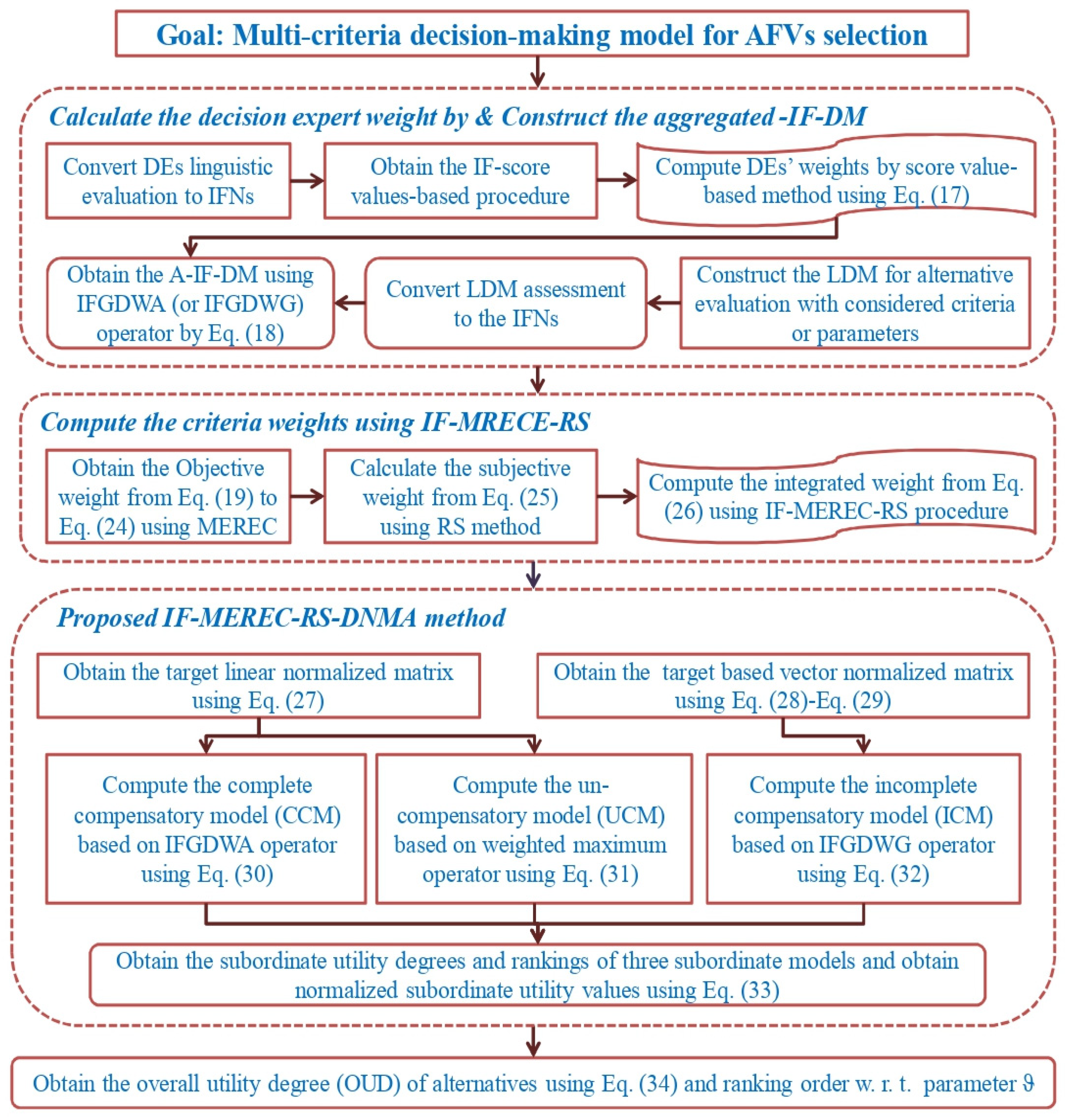
4. Proposed IF-MEREC-RS-DNMA Method

This section introduces a hybrid IF-MEREC-RS-DNMA method. The DNMA framework takes the benefits of different normalization methods and aggregation functions and combines them in an appropriate way. The procedure of the IF-MEREC-RS-DNMA methodology is displayed in the following steps (Figure 1):

Step 1: Form an “intuitionistic fuzzy-decision matrix (IF-DM)”.

In a MADA procedure, the purpose is to decide an ideal candidate from a set of m options $G=\left\{G_1,G_2,\dots ,G_m\right\}$ over the attribute set $C=\left\{C_1,C_2,\dots ,C_n\right\}$. Form a committee of experts $D=\left\{D_1,D_2,\dots ,D_l\right\}$ to elect the best option(s). Let us assume that $T={\left({\xi }_{ij}^{(k)}\right)}_{m\times n}$ is the “linguistic decision-matrix (LDM)” articulated by DEs, in which ${\xi }_{ij}^{(k)}$ implies the linguistic performance rating of an option G_i over attribute C_j given by kth expert, and further, converted into IF-DM.

Step 2: Evaluate the DEs’ weights.

In order to estimate the weights of DEs, initially the significance degrees of the DEs are supposed as “linguistic variables (LVs)” and then articulated by IFNs. Let us suppose $D_k=\left({\mu }_k,{\nu }_k\right)$ be an IFN, then the procedure for evaluating kth DE weight is as follows:

$${\lambda }_k=\frac{{\mu }_k\left(2-{\mu }_k-{\nu }_k\right)}{{\displaystyle \sum _{k=1}^l}\left[{\mu }_k\left(2-{\mu }_k-{\nu }_k\right)\right]}, k=1(1)l; {\lambda }_k\ge 0, {\displaystyle \sum _{k=1}^{\ell }{\lambda }_k=1}$$

(17)

Step 3: Determine the “aggregated IF-DM (AIF-DM)”.

In this step, all individual decision matrices are required to be combined into an AIF-DM. For this perspective, an IFGDWA (or IFGDWG) operator is employed, and then the AIF-DM is $Z={\left(z_{ij}\right)}_{m\times n}=\left({\mu }_{ij},{\nu }_{ij}\right),$ where:

$$z_{ij}=\left({\mu }_{ij},{\nu }_{ij}\right)=IFGDW{A}_{{\lambda }_k}\left({\xi }_{ij}^{\left(1\right)},{\xi }_{ij}^{\left(2\right)},\dots ,{\xi }_{ij}^{\left(l\right)}\right) \mathrm{or} IFGDW{G}_{{\lambda }_k}\left({\xi }_{ij}^{\left(1\right)},{\xi }_{ij}^{\left(2\right)},\dots ,{\xi }_{ij}^{\left(l\right)}\right).$$

(18)

Step 4: Proposed IF-MEREC-RS to the computation of attribute weight.

All the attributes are not assumed to be of the same importance. Consider $\psi ={\left({\psi }_1,{\psi }_2,\dots ,{\psi }_n\right)}^T$ to be the attribute weight with ${\displaystyle \sum _{j=1}^n{\psi }_j}=1$ and ${\psi }_j\in \left[0,1\right].$ Here, the criteria weight is computed by the combination of objective and subjective weights.

Case I: Determination of objective weights by the method of IF-MEREC.

Now, to obtain the objective weights, the classic MEREC [20] is expanded within the IFSs setting. The computational procedure of MEREC is given as follows:

Step 4.1: Normalize the AIF-DM.

To create the normalized AIF-DM $\mathbb{N}={\left({\varsigma }_{ij}\right)}_{m\times n},$ we utilize the linear normalization process, which is

$${\varsigma }_{ij}=\left({\overline{\mu }}_{ij},{\overline{\nu }}_{ij}\right)=\{\begin{array}{l}{\xi }_{ij}=\left({\mu }_{ij},{\nu }_{ij}\right), \hspace{1em}j\in C_b,\\ {\left({\xi }_{ij}\right)}^c=\left({\nu }_{ij},{\mu }_{ij}\right), j\in C_n,\end{array}$$

(19)

where C_b and C_n represent the benefit and cost-type attributes, respectively.

Step 4.2: Obtain the score-matrix.

By means of Formula (20), the score matrix $\Omega ={\left({\eta }_{ij}\right)}_{m\times n}$ of each IFN ${\varsigma }_{ij}$ is estimated

$${\eta }_{ij}=\frac{1}{2}\left(\right({\overline{\mu }}_{ij})\sum ({\overline{\nu }}_{ij})+1).$$

(20)

Step 4.3: Compute the overall performance of alternatives.

In this step, a logarithmic mapping with equivalent weights is used to determine the options’ overall performances [36]. Along with the normalized values attained in the last step, we can confirm that the lesser values of ${\eta }_{ij}$ yield the better ratings of the performances. In the following, we present the formula for computing the overall performance of the options:

$$S_i=ln\left(1+\left(\frac{1}{n}{\displaystyle \sum _j\left|ln\left({\eta }_{ij}\right)\right|}\right)\right).$$

(21)

Step 4.4: Estimate the performance of alternatives by removing each attribute.

In this following step, the options’ performances are computed by means of removing each attribute separately:

$$S_{ij}^{\prime }=ln\left(1+\left(\frac{1}{n}{\displaystyle \sum _{k,k\ne j}\left|ln\left({\eta }_{ik}\right)\right|}\right)\right).$$

(22)

Consequently, n sets of performances are obtained with respect to n criteria.

Step 4.5: Compute the summation of absolute deviations.

In this step, we calculate the removal effect of the jth criterion based on the values obtained from Steps 4.3 and 4.4. Let $V_j$ represents the effect of removing the jth attribute. We estimate the values of $V_j$ with the expression as follows:

$$V_j={\displaystyle \sum _i\left|S_{ij}^{\prime }-S_i\right|}.$$

(23)

Step 4.6: Obtain the final weights of attribute.

The final weight $w_j^o$ of the jth attribute is determined by

$$w_j^o=\frac{V_j}{{\displaystyle \sum _{j=1}^n{V}_j}}.$$

(24)

Case II: Determine the subjective weights by the IF-ranking sum (RS) weighting method.

The subjective weight-determining method permits us to reveal in the opinions and intrinsic ratings of the DEs. In this study, the RS method [38,63] is utilized to derive the subjective weights of attributes under IFS context. The procedural step is given by:

$$w_j^s=\frac{n-r_j+1}{{\displaystyle \sum _{j=1}^n\left(n-r_j+1\right)}}, j=1\left(1\right)n,$$

(25)

where $w_j^s$ determines the subjective weight of jth attribute and n signifies the number of attributes, and r_j symbolizes the rank of each attribute, where $j=1\left(1\right)n.$

Case III: Integrated weights using the IF-MEREC-RS method.

To obtain the combined weight, the DEs want to employ the subjective and objective weights in order to derive the more accurate attributes’ weights. An integrated weight-determining formula is as follows:

$$w_j=\gamma w_j^o+\left(1-\gamma \right)w_j^s,$$

(26)

where $\gamma \in \left[0, 1\right]$ is a precision objective factor of the decision strategy. In this expression, $w_j^o$ and $w_j^s$ represent the objective and subjective weights of the jth attribute, respectively.

Step 5: Assessment of the normalized AIF-DM.

Here, we discuss both the linear and vector normalization formulae. The linear normalization removes the dimensions of attributes using the principle with the interval maximum-minimum. It is utilized in the VIKOR [54] and TOPSIS [53] models. A linear normalization procedure is defined by

$${\mathbb{N}}^{\left(1\right)}={\left({\eta }_{ij}^{\left(1\right)}\right)}_{m\times n}, \mathrm{where} {\eta }_{ij}^{\left(1\right)}=\left({\overline{\mu }}_{ij}^{\left(1\right)},{\overline{\nu }}_{ij}^{\left(1\right)}\right)=\{\begin{array}{l}\frac{{\xi }_{ij}}{{\max }_i{\mathbb{S}}^{*}\left({\xi }_{ij}\right)}, \hspace{1em} j\in C_b\\ 1-\frac{{\xi }_{ij}}{{\max }_i{\mathbb{S}}^{*}\left({\xi }_{ij}\right)}, j\in C_n.\end{array}$$

(27)

Here ${\mathbb{S}}^{*}(.)$ is an improved score function of IFNs.

The vector normalization has been used in the MULTIMOORA [55] and conventional TOPSIS [64]. We utilize it to normalize the AIF-DM $\mathbb{Z}={\left(z_{ij}\right)}_{m\times n}$ with $z_{ij}=\left({\mu }_{ij},{\nu }_{ij}\right)$ into ${\mathbb{N}}^{\left(2\right)}={\left({\eta }_{ij}^{\left(2\right)}\right)}_{m\times n},$ where ${\eta }_{ij}^{\left(2\right)}=\left({\overline{\mu }}_{ij}^{\left(2\right)},{\overline{\nu }}_{ij}^{\left(2\right)}\right)$ such that

$${\eta }_{ij}^{\left(2\right)}=\{\begin{array}{l}\left({\overline{\mu }}_{ij}^{\left(2\right)}, {\overline{\nu }}_{ij}^{\left(2\right)}\right), j\in C_b,\\ \left({\overline{\nu }}_{ij}^{\left(2\right)}, {\overline{\mu }}_{ij}^{\left(2\right)}\right), j\in C_c,\end{array}$$

(28)

$${\overline{\mu }}_{ij}^{\left(2\right)}=\frac{{\mu }_{ij}}{{\left({\displaystyle \sum _{i=1}^m\left\{{\left({\mu }_{ij}\right)}^2\right\}}\right)}^{1/2}}, {\overline{\nu }}_{ij}^{\left(2\right)}=\frac{{\nu }_{ij}}{{\left({\displaystyle \sum _{i=1}^m\left\{{\left({\nu }_{ij}\right)}^2\right\}}\right)}^{1/2}}, i=1\left(1\right)m, j=1\left(1\right)n.$$

(29)

Due to the fact that both the target-based vector and linear normalization hold some benefits and restrictions simultaneously [39], they are combined in this method using various AOs in a way to achieve various utility degrees of alternatives.

Step 6: Using the subordinate aggregation models.

Here, different types of aggregation models are developed using the following normalization procedures.

Step 6.1: The “complete compensatory method (CCM)”.

The CCM can be defined based on IFGDWA operator as follows:

$${ℂ}_1\left(G_i\right)=\left({\widehat{\mu }}_{ij}^{\left(1\right)},{\widehat{\nu }}_{ij}^{\left(1\right)}\right)=IFGDW{A}_{w_j}\left({\eta }_{i1}^{\left(1\right)},{\eta }_{i2}^{\left(1\right)},\dots ,{\eta }_{in}^{\left(1\right)}\right),$$

(30)

where $w_j$ represents the attribute weight and ${\eta }_{ij}^{\left(1\right)}$ shows the target-based linear normalization value. The alternatives can be ordered by arranging ${ℂ}_1\left(G_i\right):i=1\left(1\right)m$ in a decreasing manner, and we obtain the ranking outcomes ${\rho }_1\left(G_i\right):i=1\left(1\right)m.$

Step 6.2: The “un-compensatory method (UCM)”.

For the avoidance of a situation in which the chosen solution has a very improper performance in the case of a certain criterion, the weighted maximum operator is used for the purpose of composing the second aggregation function, as shown below:

$${ℂ}_2\left(G_i\right)=\left({\widehat{\mu }}_{ij}^{\left(2\right)},{\widehat{\nu }}_{ij}^{\left(2\right)}\right)=\underset{j}{\max }{w}_j{\left({\eta }_{ij}^{\left(1\right)}\right)}^c.$$

(31)

The options can be prioritized by arranging ${ℂ}_2\left(G_i\right):i=1\left(1\right)m$ in a decreasing way, and we obtain the ranking outcomes ${\rho }_2\left(G_i\right):i=1\left(1\right)m.$

Step 6.3: The “incomplete compensatory method (ICM)”.

We utilize the vector normalization of the third aggregation procedure by the IFGDWG operator:

$${ℂ}_3\left(G_i\right)=\left({\widehat{\mu }}_{ij}^{\left(3\right)},{\widehat{\nu }}_{ij}^{\left(3\right)}\right)=IFGDW{G}_{w_j}\left({\eta }_{i1}^{\left(2\right)},{\eta }_{i2}^{\left(2\right)},\dots ,{\eta }_{in}^{\left(2\right)}\right)$$

(32)

where $w_j$ signifies the attribute weight and ${\eta }_{ij}^{\left(2\right)}$ denotes the target-based vector normalized value. The alternatives can be arranged by listing ${ℂ}_3\left(G_i\right):i=1\left(1\right)m$ in a descending manner, and we obtain the ranking outcomes ${\rho }_3\left(G_i\right):i=1\left(1\right)m.$

Step 7: Combination of subordinate “utility degrees (UDs)” and priority orders.

The last phase necessitates the achievement of all-inclusive ranking by combining the outcomes of the given three models. These are considered as the following three parameters or attributes: CCM $\left({\mathbb{Q}}_1\right),$ UCM $\left({\mathbb{Q}}_2\right)$ and ICM $\left({\mathbb{Q}}_3\right).$ Each option $G_i$ has two kinds of degrees, the “utility degree (UD)” ${ℂ}_{\tau }\left(G_i\right):i=1\left(1\right)m$, and the preference order ${\rho }_{\tau }\left(G_i\right):i=1\left(1\right)m$ over each attribute ${\mathbb{Q}}_{\tau }:\tau =1,2,3$. Evidently, we generate two “decision matrices (DMs)”, which are the UD-DM $ƛ(ℂ)={\left[{ℂ}_{\tau }\left(G_i\right)\right]}_{m\times 3}$ and the ranking-DM $ƛ\left(\rho \right)={\left[{\rho }_{\tau }\left(G_i\right)\right]}_{m\times 3}.$

To preserve the inventive assessment of the subordinate UDs ${ℂ}_{\tau }\left(G_i\right):\tau =1,2,3,$ the normalized versions are given by

$${ℂ}_{\tau }^{\left(N\right)}\left(G_i\right)=\left({\widehat{\mu }}_{ij}^{\left(N\right)},{\widehat{\nu }}_{ij}^{\left(N\right)}\right); \tau =1,2,3,$$

$$\begin{array}{c}\mathrm{where} {\widehat{\mu }}_{ij}^{\left(N\right)}=\frac{{\widehat{\mu }}_{ij}^{\left(\tau \right)}}{{\left({\displaystyle \sum _{i=1}^m\left\{{\left({\widehat{\mu }}_{ij}^{\left(\tau \right)}\right)}^2\right\}}\right)}^{1/2}},{\widehat{\nu }}_{ij}^{\left(N\right)}=\frac{{\widehat{\nu }}_{ij}^{\left(\tau \right)}}{{\left({\displaystyle \sum _{i=1}^m\left\{{\left({\widehat{\nu }}_{ij}^{\left(\tau \right)}\right)}^2\right\}}\right)}^{1/2}},\\ \tau =1,2,3, i=1\left(1\right)m, j=1\left(1\right)n.\end{array}$$

(33)

Step 8: Compute the “overall utility degree (OUD)” of each option.

A parameter $\vartheta \in \left[0,1\right]$ is taken to show the subordinate UDs and the subordinate preferences of options. Here, we take $\vartheta =0.5$.

The OUD of each option is presented by

$$\begin{array}{c}{ℝ}_i=[\frac{1}{2}(w_1\ast \sqrt{\vartheta {\left({ℂ}_1^{\left(N\right)}\left(G_i\right)/{\max }_i{ℂ}_1^{\left(N\right)}\left(G_i\right)\right)}^2+\left(1-\vartheta \right){\left(\frac{m-{\rho }_1\left(G_i\right)+1}{m}\right)}^2}\\ -w_2\ast \sqrt{\vartheta {\left({ℂ}_2^{\left(N\right)}\left(G_i\right)/{\max }_i{ℂ}_2^{\left(N\right)}\left(G_i\right)\right)}^2+\left(1-\vartheta \right){\left(\frac{{\rho }_2\left(G_i\right)}{m}\right)}^2}\\ +w_3\ast \sqrt{\vartheta {\left({ℂ}_3^{\left(N\right)}\left(G_i\right)/{\max }_i{ℂ}_3^{\left(N\right)}\left(G_i\right)\right)}^2+\left(1-\vartheta \right){\left(\frac{m-{\rho }_3\left(G_i\right)+1}{m}\right)}^2})+1],\end{array}$$

(34)

where $w_1,$ $w_2$ and $w_3$ are the weight of the CCM, UCM, and ICM, respectively, such that $w_1+w_2+w_3=1$. Here, the weights $w_1,$ $w_2$ and $w_3$ are obtained using the developed IF-RS method, or provide equal weights. The ultimate preference set $\rho =\left\{\rho \left(G_1\right),\rho \left(G_2\right),\rho \left(G_3\right),\dots ,\rho \left(G_m\right)\right\}$ is obtained in decreasing order of ${ℝ}_i:i=1\left(1\right)m.$

Step 9: End.

5. Case Study: Assessment of Alternative Fuel Vehicles (AFVs)

Due to rising oil import bills and a diminishing stock of fossil-based fuels, the search for cleaner and safer alternative fuels is now the leading challenge being faced by scientists and decision makers in India. Recent years have seen a noticeable shift towards the use of renewable and alternative fuels, moving away from conventional fossil-based fuels. In recent times, the progress of AFVs has become gradually more important worldwide. One of the most significant causes for this increase is that AFVs are seen as a valuable way of dealing with climate change, shifting energy consumption to produce less carbon and less pollution, and because they offer more energy diversity.

To display the effectiveness and applicability of the proposed approach, a case study related to the AFV selection problem for a private home healthcare service provider (XYZ), situated in Chandigarh, India, is presented. In this region, the selected healthcare service provider serves the patients within a 45 miles radius of Chandigarh. The healthcare service provider requires a passenger car to carry the patients from their home. In the current section, we have concentrated on the development and implementation of a new model that will help the service provider to assess and choose a suitable AFV option.

In real-life situations, it is very difficult to evaluate the exact criteria for AFV evaluation problems, due to lack of precise knowledge/information, increasing complexity, and time-limitations. To evaluate the criteria and alternatives, we created a panel of four DEs, who are experts in sustainable development, internal combustion engines and, the automotive industry in India. Two of them are from the automotive industry, one expert is from the internal combustion engine sector, and the other is from the field of sustainable development. The qualifications of three experts are Ph.D. and the other is a master’s degree holder working at Autonomous Intelligence Motors Private Limited, India. The DEs collaborated with the authors during the entire study.

Furthermore, the panel of decision experts participated in an online questionnaire in order to determine the importance of criteria in the selection of AFV alternatives. The significant goal of this questionnaire is to discuss the potential factors/criteria influencing the AFV selection. The criteria that may affect the AFV selection were collected by reviewing the literature. Based on the literature review, online questionnaire and open interviews, a set of sustainability perspectives, and indicators were collected to choose the best AFVs. After that, five main dimensions of criteria were considered, namely the environmental, technical, economic, social, and political dimensions [5,46].

In the meantime, based on the accessibility of vehicle models suitable for this fleet operation and the availability of fuel, a panel of experts considered five AFVs, namely hybrid electric vehicles (G₁), electric vehicles (G₂), hydrogen vehicles (G₃), natural gas vehicles (G₄), and biofuel vehicles (G₅). In addition, open interviews and literature reviews facilitated us to recognize global AFVs. On account of the initial analysis, extant literature, and discussion with experts, 15 attributes have been recognized, as shown in

Table 1. Description of considered criteria for the AFVs.

Dimension	Criteria	Meaning	References
Economic (L1)	Purchase cost (C1)	The marketing cost of a specific vehicle (containing taxes)	[2,65,66,67,68,69]
	Energy cost (C2)	Energy generation and supply cost	[42,65,66,67,70,71]
	Maintenance cost (C3)	The cost needed for systematic maintenance of the vehicle	[1,2,43,71]
Social (L2)	Sense of comfort (C4)	The consumer’s consideration to the comfort and accessories of the vehicle	[5,72]
	Job creation (C5)	The formation of new workplaces	[1,5,71,73]
	Social benefits (C6)	The increase in the level of welfare and lifestyle of the society	[42,71,74]
	Social acceptability (C7)	The choice of a client for purchasing a particular vehicle	[1,65,74,75,76]
Environmental (L3)	Noise pollution (C8)	Noise when the vehicle is operating	[73,75,77]
	Environmental-friendly technology (C9)	The degree of option fuel usability while driving the vehicle	[65,78,79]
Technological (L4)	Fueling/charging Infrastructure (C10)	AFV fuel station sites	[42,66,72,73,74]
	Driving range (C11)	Range that can be reached from a single charge	[2,42,68,69,72]
	Energy efficiency (C12)	Efficiency of fuel energy	[70,73,80]
Political (L5)	Energy security (C13)	Dependence on non-fossil methods	[5,71,74]
	Policy support (C14)	Flexible policy procedures and guidelines	[65,71]
	Financial incentives (C15)	Government aids	[1,5,42]

. Afterward, DEs are invited to give their opinions and experiences, both to weigh the evaluation criteria and to score the candidate AFVs by means of each criterion. As per their domain knowledge, DEs express their preferences in the form of LVs.

Steps 1–3:

Table 2. Rating of DEs in form of LVs for AFVs.

LVs	IFNs
Extremely Significance	(0.90, 0.10)
Very Significance	(0.80, 0.15)
Significance	(0.70, 0.25)
Moderate	(0.50, 0.45)
Insignificance	(0.40, 0.55)
Very Insignificance	(0.20, 0.75)
Extremely Insignificance	(0.10, 0.90)

and

Table 3. LVs for rating of alternatives over criteria for AFVs.

LVs	IFNs
Extremely good/high (EH)	(0.95, 0.05)
Very very good//high (VVH)	(0.85, 0.10)
Very good/high (VH)	(0.80, 0.15)
Good/high (H)	(0.70, 0.20)
Slightly good/high (MH)	(0.60, 0.30)
Average (A)	(0.50, 0.40)
Slightly low (ML)	(0.40, 0.50)
Low (L)	(0.30, 0.60)
Very very low (VL)	(0.20, 0.70)
Very low (VVL)	(0.10, 0.80)
Extremely low (EL)	(0.05, 0.95)

adopted from Kumari and Mishra [81], to present the importance of the DEs and criteria to estimate the significance ratings of the DEs and the assessment criteria for AFVs, which were then articulated in terms of IFNs. Using Table 2 and Equation (17), the DEs’ weights are calculated and portrayed in

Table 4. The weights of DEs for AFVs.

DEs	D1	D2	D3	D4
LVs	VS (0.80, 0.15)	S (0.70, 0.25)	M (0.50, 0.45)	ES (0.90, 0.10)
Weight	0.2800	0.2450	0.1750	0.3000

.

Table 5. LDM for AFVs by DEs.

Criteria	G1	G2	G3	G4	G5
C1	(L, VL, VL, ML)	(L, ML, VL, L)	(A, ML, A, L)	(ML, ML, A, L)	(A, A, ML, ML)
C2	(ML, L, A, L)	(VL, L, VL, ML)	(MH, A, ML, A)	(VL, L, ML, L)	(VVL, L, ML, ML)
C3	(L, L, L, VL)	(VL, ML, VL, A)	(A, L, A, ML)	(ML, L, A, A)	(A, A, ML, L)
C4	(A, MH, MH, H)	(H, H, H, MH)	(MH, MH, A, H)	(H, ML, VH, VH)	(MH, A, MH, ML)
C5	(MH, H, A, MH)	(VH, H, VH, A)	(ML, MH, A, MH)	(VH, ML, A, MH)	(MH, MH, H, VH)
C6	(A, ML, VH, A)	(L, ML, A, H)	(H, VH, A, MH)	(A, MH, A, H)	(MH, A, ML, A)
C7	(MH, L, A, VVH)	(A, L, ML, MH)	(MH, A, VH, H)	(VVH, H, A, MH)	(VVH, A, H, VH)
C8	(VL, L, A, ML)	(A, VL, L, ML)	(A, MH, VL, L)	(VL, ML, VL, ML)	(A, ML, ML, L)
C9	(A, H, MH, H)	(VVH, H, H, A)	(MH, H, A, H)	(MH, H, A, MH)	(ML, A, MH, VH)
C10	(VVH, H, A, MH)	(MH, H, VH, H)	(ML, MH, A, VH)	(H, ML, A, H)	(MH, H, VH, VH)
C11	(ML, A, VL, ML)	(A, ML, MH, H)	(H, A, H, VVH)	(MH, ML, A, VH)	(A, A, MH, H)
C12	(H, ML, A, MH)	(VH, MH, A, MH)	(VH, A, MH, ML)	(ML, MH, VH, H)	(VH, VH, H, MH)
C13	(VH, H, VH, A)	(H, VH, VH, MH)	(MH, ML, A, MH)	(MH, VH, MH, H)	(A, ML, MH, VH)
C14	(A, H, MH, H)	(H, H, VVH, A)	(VH, MH, A, H)	(VHH, A, ML, ML)	(ML, A, MH, MH)
C15	(H, MH, A, VH)	(VH, H, MH, MH)	(ML, H, A, A)	(VH, H, A, H)	(MH, ML, H, A)

represents the LDM by DEs for each option AFV G_i over the different attributes. From Equation (18) and Table 5, the AIF-DM is computed (taking p = 1 and q = 1) and shown in

Table 6. AIF-DM for AFVs.

Criteria	G1	G2	G3	G4	G5
C1	(0.342, 0.578, 0.080)	(0.340, 0.575, 0.086)	(0.444, 0.473, 0.083)	(0.411, 0.504, 0.086)	(0.460, 0.445, 0.094)
C2	(0.398, 0.523, 0.078)	(0.341, 0.580, 0.079)	(0.517, 0.386, 0.096)	(0.327, 0.588, 0.084)	(0.362, 0.555, 0.083)
C3	(0.286, 0.618, 0.096)	(0.417, 0.514, 0.069)	(0.446, 0.469, 0.085)	(0.448, 0.467, 0.085)	(0.451, 0.466, 0.083)
C4	(0.606, 0.292, 0.102)	(0.672, 0.227, 0.101)	(0.616, 0.282, 0.102)	(0.699, 0.228, 0.074)	(0.527, 0.379, 0.094)
C5	(0.610, 0.288, 0.101)	(0.700, 0.222, 0.077)	(0.538, 0.368, 0.095)	(0.613, 0.306, 0.081)	(0.685, 0.230, 0.084)
C6	(0.549, 0.366, 0.085)	(0.524, 0.394, 0.082)	(0.669, 0.299, 0.031)	(0.590, 0.308, 0.102)	(0.517, 0.386, 0.096)
C7	(0.637, 0.286, 0.076)	(0.495, 0.422, 0.083)	(0.650, 0.258, 0.092)	(0.695, 0.217, 0.088)	(0.742, 0.186, 0.072)
C8	(0.397, 0.530, 0.073)	(0.418, 0.507, 0.075)	(0.477, 0.453, 0.070)	(0.366, 0.553, 0.081)	(0.424, 0.492, 0.084)
C9	(0.632, 0.265, 0.103)	(0.701, 0.211, 0.088)	(0.641, 0.256, 0.102)	(0.610, 0.288, 0.101)	(0.606, 0.315, 0.079)
C10	(0.695, 0.217, 0.088)	(0.694, 0.215, 0.091)	(0.612, 0.308, 0.080)	(0.608, 0.292, 0.100)	(0.727, 0.198, 0.075)
C11	(0.424, 0.491, 0.085)	(0.568, 0.335, 0.098)	(0.714, 0.199, 0.087)	(0.618, 0.302, 0.080)	(0.584, 0.315, 0.102)
C12	(0.576, 0.327, 0.098)	(0.649, 0.265, 0.085)	(0.598, 0.322, 0.080)	(0.630, 0.282, 0.088)	(0.731, 0.197, 0.073)
C13	(0.700, 0.222, 0.077)	(0.720, 0.202, 0.078)	(0.543, 0.361, 0.095)	(0.686, 0.227, 0.088)	(0.608, 0.312, 0.080)
C14	(0.632, 0.265, 0.103)	(0.681, 0.225, 0.094)	(0.679, 0.235, 0.086)	(0.595, 0.325, 0.080)	(0.530, 0.375, 0.095)
C15	(0.681, 0.234, 0.085)	(0.688, 0.227, 0.086)	(0.536, 0.368, 0.096)	(0.702, 0.212, 0.086)	(0.551, 0.352, 0.097)

.

Step 4: To compute the objective weights of criteria by MEREC, firstly the normalized AIF-DM is computed with the use of Equation (19). Next, the overall performances of the options based on Equation (20) are determined and presented as S₁ = 0.370, S₂ = 0.353, S₃ = 0.404, S₄ = 0.358 and S₅ = 0.389. By means of Equation (21), the overall performance of each option by removing each attribute is computed and shown in

Table 7. Results by MEREC for attributes’ weights computation.

Criteria	$\left({\mathit{S}}_{\mathit{i}\mathit{j}}^{\prime }\right)\mathbf{Values}$					Vj	wj
	G1	G2	G3	G4	G5
C1	0.347	0.330	0.375	0.329	0.357	0.136	0.0863
C2	0.343	0.330	0.367	0.336	0.366	0.133	0.0840
C3	0.351	0.324	0.374	0.326	0.358	0.141	0.0891
C4	0.350	0.337	0.386	0.343	0.364	0.093	0.0588
C5	0.350	0.339	0.380	0.338	0.375	0.092	0.0583
C6	0.345	0.326	0.388	0.337	0.363	0.116	0.0732
C7	0.351	0.323	0.388	0.343	0.378	0.090	0.0568
C8	0.343	0.324	0.372	0.333	0.361	0.141	0.0894
C9	0.352	0.339	0.388	0.338	0.370	0.088	0.0554
C10	0.356	0.339	0.385	0.338	0.377	0.079	0.0502
C11	0.334	0.330	0.392	0.338	0.369	0.112	0.0706
C12	0.348	0.335	0.384	0.339	0.377	0.090	0.0570
C13	0.356	0.340	0.381	0.343	0.370	0.085	0.0540
C14	0.352	0.338	0.390	0.336	0.364	0.094	0.0593
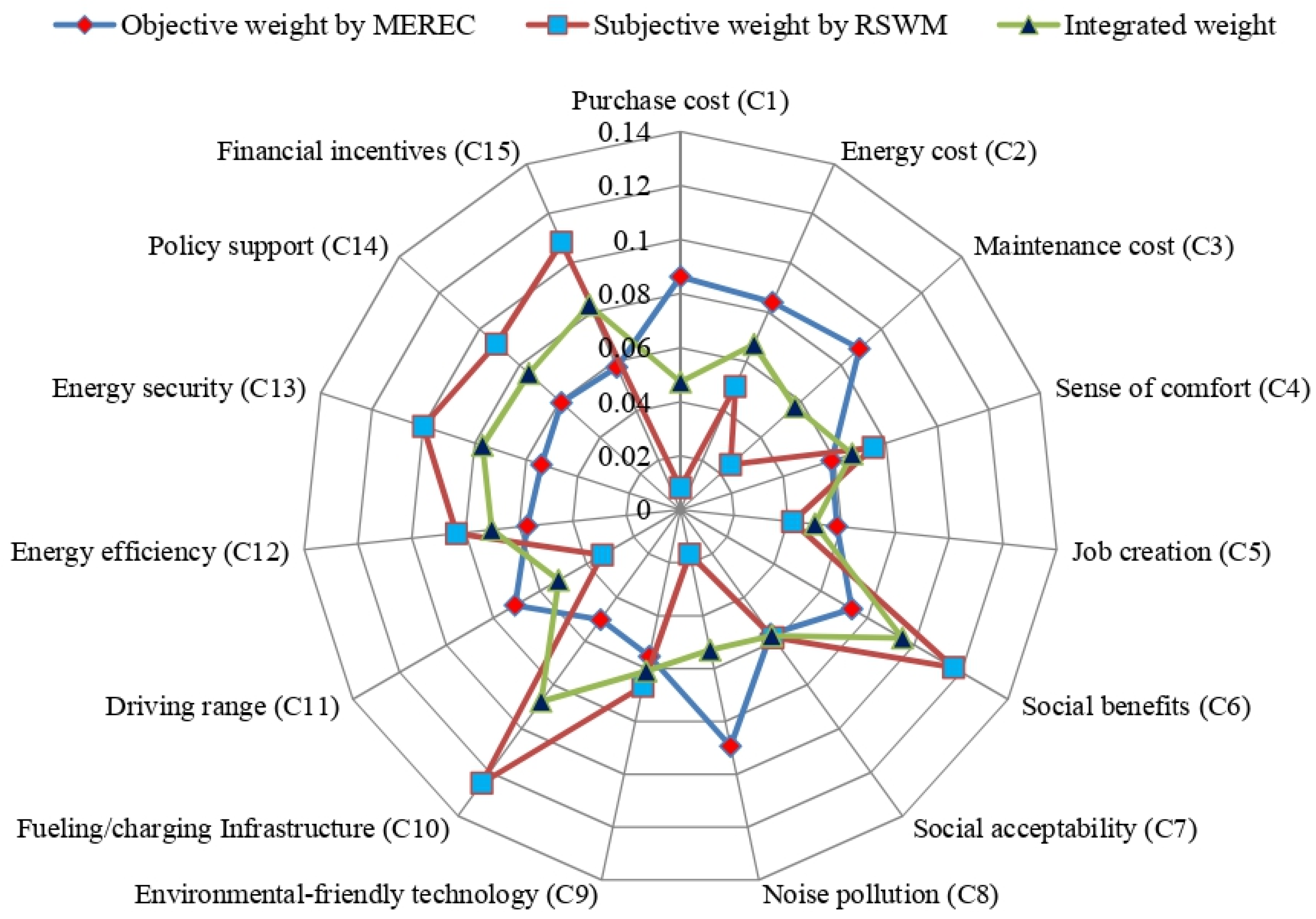
C15	0.355	0.338	0.380	0.344	0.366	0.091	0.0577

. Next, we derive the removal effect of each attribute on the overall performance of the options using Equation (22). Furthermore, we calculate the final attributes’ weights for AFV selection by utilizing Equations (23) and (24), and given in last column of Table 7. The resultant values are in depicted in Figure 2.

From Equation (25), we have calculated the subjective weights using the IF-RS weighting method of each criterion for AFVs selection. The required results are shown in

Table 8. Weights of criteria for AFVs selection using the RS method.

Criteria	D1	D2	D3	D4	Aggregated IFNs	$\mathbf{Crisp} \mathbf{Values} {\mathbb{S}}^{*}\left({\tilde{\mathit{\xi }}}_{\mathit{k}\mathit{j}}\right)$	Rank of Challenges	$\mathbf{Weight} {\mathit{w}}_{\mathit{j}}^{\mathit{s}}$
C1	MH	A	ML	MH	(0.548, 0.355, 0.097)	0.403	15	0.0083
C2	A	A	ML	L	(0.451, 0.466, 0.083)	0.508	10	0.0500
C3	A	MH	L	A	(0.509, 0.401, 0.090)	0.446	13	0.0250
C4	MH	L	ML	A	(0.493, 0.424, 0.083)	0.534	7	0.0750
C5	L	MH	L	ML	(0.453, 0.476, 0.071)	0.488	11	0.0417
C6	A	H	MH	A	(0.572, 0.326, 0.101)	0.623	2	0.1167
C7	ML	A	H	L	(0.490, 0.472, 0.038)	0.509	9	0.0583
C8	MH	A	L	MH	(0.544, 0.366, 0.090)	0.411	14	0.0167
C9	A	ML	MH	ML	(0.477, 0.432, 0.091)	0.522	8	0.0667
C10	H	ML	A	MH	(0.576, 0.327, 0.098)	0.624	1	0.1250
C11	L	VL	MH	ML	(0.431, 0.504, 0.064)	0.464	12	0.0333
C12	ML	MH	MH	A	(0.525, 0.381, 0.095)	0.572	6	0.0833
C13	H	ML	L	MH	(0.560, 0.352, 0.088)	0.604	4	0.1000
C14	H	L	ML	MH	(0.558, 0.356, 0.086)	0.601	5	0.0917
C15	MH	H	L	A	(0.567, 0.341, 0.092)	0.613	3	0.1083

, and depicted in Figure 2.

To derive the combined weights of attributes, we have combined the results obtained by the IF-MEREC for objective weighting and the IF-RS method for subjective weighting by means of Equation (26). The final weight for $\tau =0.5$ is shown in Figure 2 and given as follows:

w_j = (0.0473, 0.0670, 0.0570, 0.0669, 0.0500, 0.0949, 0.0576, 0.0530, 0.0610, 0.0876, 0.0520, 0.0702, 0.0770, 0.0755, 0.0830).

Here, Figure 2 displays the significance value or weights of different criteria of AFV selection for sustainable road transportation with respect to the goal. The parameter social benefits (C₆), with a weight value of 0.0949, have been determined to be the most important parameter in AFV selection. Fueling/charging infrastructure (C₁₁), with a weight value of 0.0876, is the second most important parameter in AFV selection. Financial incentives (C₁₅), with a significance value of 0.0830, is the third most significant parameter in AFV selection, and others are considered as crucial parameters in AFV selection for sustainable road transportation.

Step 5: According to the Equations (27)–(29) and Table 6, the linear and vector normalization values for AFV selection are estimated and given in

Table 9. Linear normalization matrix for AFVs selection.

Criteria	G1	G2	G3	G4	G5
C1	(0.228, 0.713, 0.059)	(0.226, 0.710, 0.064)	(0.304, 0.630, 0.066)	(0.279, 0.654, 0.067)	(0.317, 0.606, 0.077)
C2	(0.274, 0.665, 0.061)	(0.231, 0.709, 0.059)	(0.368, 0.549, 0.083)	(0.221, 0.716, 0.063)	(0.247, 0.690, 0.063)
C3	(0.201, 0.726, 0.074)	(0.302, 0.642, 0.056)	(0.325, 0.604, 0.071)	(0.326, 0.602, 0.071)	(0.329, 0.601, 0.070)
C4	(0.496, 0.404, 0.099)	(0.559, 0.336, 0.105)	(0.505, 0.395, 0.100)	(0.586, 0.337, 0.077)	(0.423, 0.490, 0.087)
C5	(0.502, 0.399, 0.099)	(0.590, 0.329, 0.081)	(0.434, 0.478, 0.088)	(0.504, 0.417, 0.079)	(0.575, 0.338, 0.088)
C6	(0.420, 0.503, 0.077)	(0.399, 0.528, 0.073)	(0.531, 0.438, 0.031)	(0.457, 0.446, 0.096)	(0.393, 0.521, 0.086)
C7	(0.546, 0.378, 0.076)	(0.412, 0.511, 0.077)	(0.558, 0.348, 0.094)	(0.603, 0.305, 0.092)	(0.652, 0.270, 0.078)
C8	(0.259, 0.686, 0.055)	(0.274, 0.669, 0.057)	(0.319, 0.625, 0.056)	(0.237, 0.703, 0.060)	(0.279, 0.656, 0.064)
C9	(0.525, 0.372, 0.103)	(0.593, 0.313, 0.093)	(0.534, 0.363, 0.103)	(0.504, 0.396, 0.100)	(0.500, 0.422, 0.077)
C10	(0.596, 0.311, 0.092)	(0.596, 0.308, 0.096)	(0.516, 0.406, 0.078)	(0.512, 0.390, 0.098)	(0.630, 0.289, 0.081)
C11	(0.342, 0.583, 0.075)	(0.470, 0.437, 0.093)	(0.612, 0.295, 0.093)	(0.517, 0.404, 0.079)	(0.485, 0.416, 0.098)
C12	(0.482, 0.424, 0.094)	(0.553, 0.361, 0.086)	(0.503, 0.419, 0.078)	(0.534, 0.378, 0.088)	(0.635, 0.287, 0.078)
C13	(0.599, 0.320, 0.081)	(0.619, 0.298, 0.083)	(0.448, 0.462, 0.090)	(0.584, 0.324, 0.091)	(0.509, 0.413, 0.078)
C14	(0.517, 0.381, 0.102)	(0.565, 0.338, 0.097)	(0.563, 0.348, 0.089)	(0.482, 0.441, 0.077)	(0.423, 0.490, 0.087)
C15	(0.573, 0.339, 0.088)	(0.580, 0.331, 0.089)	(0.436, 0.475, 0.090)	(0.594, 0.315, 0.091)	(0.450, 0.459, 0.091)

and

Table 10. Vector normalization matrix for AFV selection.

Criteria	G1	G2	G3	G4	G5
C1	(0.3800, 0.4995, 0.1205)	(0.3774, 0.4965, 0.1261)	(0.4931, 0.4087, 0.0983)	(0.4565, 0.4349, 0.1087)	(0.5116, 0.3845, 0.1039)
C2	(0.4508, 0.4402, 0.1089)	(0.3861, 0.4877, 0.1262)	(0.5855, 0.3248, 0.0898)	(0.3704, 0.4949, 0.1347)	(0.4095, 0.4669, 0.1236)
C3	(0.3088, 0.5415, 0.1497)	(0.4505, 0.4504, 0.0991)	(0.4810, 0.4114, 0.1075)	(0.4832, 0.4096, 0.1072)	(0.4866, 0.4085, 0.1049)
C4	(0.4327, 0.4547, 0.1126)	(0.4792, 0.3538, 0.1669)	(0.4395, 0.4400, 0.1205)	(0.4986, 0.3549, 0.1466)	(0.3759, 0.5904, 0.0337)
C5	(0.4318, 0.4481, 0.1201)	(0.4955, 0.3454, 0.1590)	(0.3803, 0.5714, 0.0482)	(0.4337, 0.4749, 0.0913)	(0.4850, 0.3574, 0.1576)
C6	(0.4284, 0.4641, 0.1075)	(0.4094, 0.4993, 0.0914)	(0.5227, 0.3793, 0.0980)	(0.4609, 0.3901, 0.1489)	(0.4040, 0.4892, 0.1068)
C7	(0.4390, 0.4478, 0.1131)	(0.3409, 0.6508, 0.0083)	(0.4478, 0.4035, 0.1488)	(0.4786, 0.3401, 0.1813)	(0.5114, 0.2904, 0.1981)
C8	(0.4251, 0.4663, 0.1086)	(0.4469, 0.4467, 0.1065)	(0.5101, 0.3989, 0.0909)	(0.3916, 0.4863, 0.1221)	(0.4539, 0.4329, 0.1132)
C9	(0.4424, 0.4405, 0.1171)	(0.4906, 0.3499, 0.1595)	(0.4488, 0.4258, 0.1254)	(0.4270, 0.4790, 0.0940)	(0.4240, 0.5223, 0.0536)
C10	(0.4644, 0.3887, 0.1469)	(0.4639, 0.3840, 0.1520)	(0.4093, 0.5508, 0.0399)	(0.4065, 0.5226, 0.0708)	(0.4861, 0.3535, 0.1604)
C11	(0.3220, 0.6429, 0.0351)	(0.4311, 0.4385, 0.1304)	(0.5422, 0.2611, 0.1967)	(0.4690, 0.3956, 0.1354)	(0.4433, 0.4120, 0.1447)
C12	(0.4027, 0.5177, 0.0796)	(0.4545, 0.4199, 0.1256)	(0.4185, 0.5099, 0.0716)	(0.4410, 0.4458, 0.1132)	(0.5115, 0.3114, 0.1772)
C13	(0.4783, 0.3658, 0.1559)	(0.4915, 0.3331, 0.1755)	(0.3712, 0.5942, 0.0346)	(0.4683, 0.3731, 0.1586)	(0.4154, 0.5129, 0.0718)
C14	(0.4516, 0.4082, 0.1402)	(0.4866, 0.3465, 0.1669)	(0.4850, 0.3614, 0.1537)	(0.4249, 0.4996, 0.0754)	(0.3789, 0.5771, 0.0440)
C15	(0.4792, 0.3649, 0.1560)	(0.4838, 0.3538, 0.1623)	(0.3771, 0.5743, 0.0487)	(0.4937, 0.3311, 0.1753)	(0.3879, 0.5498, 0.0623)

.

Step 6: The subordinate utility degrees of the CCM, UCM and ICM are estimated by Equations (30)–(32), and portrayed in

Table 11. The CCM, UCM and ICM degrees for each option.

Options	$\mathbf{CCM} \left({\mathit{\mathbb{Q}}}_1\right)$		$\mathbf{UCM} \left({\mathit{\mathbb{Q}}}_2\right)$		$\mathbf{ICM}\left({\mathit{\mathbb{Q}}}_3\right)$
	${\mathit{ℂ}}_1\left({\mathit{G}}_{\mathit{i}}\right)$	${\mathbb{S}}^{*}\left({\mathit{ℂ}}_1\left({\mathit{G}}_{\mathit{i}}\right)\right)$	${\mathit{ℂ}}_2\left({\mathit{G}}_{\mathit{i}}\right)$	${\mathbb{S}}^{*}\left({\mathit{ℂ}}_2\left({\mathit{G}}_{\mathit{i}}\right)\right)$	${\mathit{ℂ}}_3\left({\mathit{G}}_{\mathit{i}}\right)$	${\mathbb{S}}^{*}\left({\mathit{ℂ}}_3\left({\mathit{G}}_{\mathit{i}}\right)\right)$
G1	(0.566, 0.350, 0.084)	0.608	(0.071, 0.913, 0.016)	0.079	(0.450, 0.426, 0.124)	0.512
G2	(0.581, 0.337, 0.082)	0.622	(0.079, 0.907, 0.014)	0.086	(0.462, 0.401, 0.137)	0.530
G3	(0.534, 0.386, 0.080)	0.574	(0.052, 0.933, 0.015)	0.059	(0.430, 0.468, 0.102)	0.481
G4	(0.571, 0.346, 0.083)	0.613	(0.081, 0.904, 0.015)	0.088	(0.456, 0.415, 0.129)	0.521
G5	(0.551, 0.368, 0.081)	0.591	(0.075, 0.910, 0.014)	0.082	(0.435, 0.449, 0.116)	0.493

.

Step 7: Corresponding to Equation (33), the normalized degrees of the subordinate UDs of CCM, UCM, and ICM are estimated, and their preferences are also obtained and are shown in

Table 12. Normalized CCM, UCM and ICM degrees and OUDs for AFVs selection.

Options	$\mathbf{CCM} \left({\mathit{\mathbb{Q}}}_1\right)$		$\mathbf{UCM} \left({\mathit{\mathbb{Q}}}_2\right)$		$\mathbf{ICM} \left({\mathit{\mathbb{Q}}}_3\right)$		${\mathit{ℝ}}_{\mathit{i}}$$\left(\mathit{\xi }=0.5\right)$	Final Ranking
	${\mathit{ℂ}}_1^{\left(\mathit{N}\right)}\left({\mathit{G}}_{\mathit{i}}\right)$	${\mathit{\rho }}_1\left({\mathit{G}}_{\mathit{i}}\right)$	${\mathit{ℂ}}_2^{\left(\mathit{N}\right)}\left({\mathit{G}}_{\mathit{i}}\right)$	${\mathit{\rho }}_2\left({\mathit{G}}_{\mathit{i}}\right)$	${\mathit{ℂ}}_3^{\left(\mathit{N}\right)}\left({\mathit{G}}_{\mathit{i}}\right)$	${\mathit{\rho }}_3\left({\mathit{G}}_{\mathit{i}}\right)$
G1	0.452	3	0.444	2	0.451	3	0.654	2
G2	0.462	1	0.484	4	0.467	1	0.685	1
G3	0.427	5	0.332	1	0.423	5	0.638	3
G4	0.455	2	0.495	5	0.459	2	0.632	4
G5	0.439	4	0.462	3	0.434	4	0.610	5
Weight of aggregation model	$w_1=1/3$		$w_2=1/3$		$w_3=1/3$

. Next, the normalized subordinate UDs and the weights of subordinate UDs are calculated and mentioned in Table 10.

Step 8: From Equation (34), the subordinate normalized UDs and ranks, the OUDs and the final preference orders of options are obtained and depicted in Table 12. Regardless of assuming $w_1=w_2=w_3=1/3,$ the weights can be chosen as per the preferences of DEs on the basis of the comprehensive accomplishment by the alternatives or of their poor performances. CCM is preferred if the attention of the alternatives’ comprehensive abilities can be drawn from DEs. If the DEs are not interested in taking risks, then a large weight can be attached to the UCM. It is pertinent to mention that ICM can be endowed by a large weight in cases when the DEs focus solely upon comprehensive performance as well as decision risks. Hence, the preference order of options is $G_2\succ G_1\succ G_3\succ G_4\succ G_5$, and the option G₂ is with a highest UD of appropriateness of options.

5.1. Comparative Study

In the current part of the study, a comparison is made between the outcomes obtained from the IF-MEREC-RS-DNMA method and those from other MCDM models. To demonstrate the efficiency and show the unique advantages of the IF-MEREC-RS-DNMA framework, we compare the present approach with the previously developed approaches, which are the “intuitionistic fuzzy complex proportional assessment (IF-COPRAS)” [82] and the “intuitionistic fuzzy weighted aggregated sum product assessment (IF-WASPAS)” method [83].

5.1.1. IF-COPRAS Method

To show the comparison, we choose the IF-COPRAS model given by Gitinavard and Shirazi [82] with the analysis of decision-making problem given in above section.

Steps 1–4: Same as earlier method.

Step 5: Add the values of attributes for benefit and cost.

In this step, to calculate the values of ${\alpha }_i$ and ${\beta }_i$ for benefit and cost-type criteria, we implement the following procedure:

$${\alpha }_i=\underset{j=1}{\overset{l}{\oplus }}{w}_j{z}_{ij}, i=1\left(1\right)m$$

(35)

$${\beta }_i=\underset{j=l+1}{\overset{n}{\oplus }}{w}_j{z}_{ij}, i=1\left(1\right)m.$$

(36)

In these formulae, $l$ is number of benefit-type attributes, while n is the whole criteria.

Step 6: Calculate the “relative degree (RD)” of each option.

The RD ${\gamma }_i$ of the ith option is computed by

$${\gamma }_i={\mathbb{S}}^{*}\left({\alpha }_i\right)+\frac{\underset{i}{\min }{\mathbb{S}}^{*}\left({\beta }_i\right){\displaystyle \sum _{i=1}^m{\mathbb{S}}^{*}\left({\beta }_i\right)}}{{\mathbb{S}}^{*}\left({\beta }_i\right){\displaystyle \sum _{i=1}^m\frac{\underset{i}{\min }{\mathbb{S}}^{*}\left({\beta }_i\right)}{{\mathbb{S}}^{*}\left({\beta }_i\right)}}},i=1\left(1\right)m.$$

(37)

Here, ${\mathbb{S}}^{*}\left({\alpha }_i\right)$ and ${\mathbb{S}}^{*}\left({\beta }_i\right)$ denote the score degrees of ${\alpha }_i$ and ${\beta }_i,$ respectively.

Step 7: Compute the “utility degree (UD)” of each option.

The formula for the computation of the utility degree ${\delta }_i$ of each option is

$${\delta }_i=\frac{{\gamma }_i}{{\gamma }_{\max }}\times 100\%,i=1\left(1\right)m.$$

(38)

Step 8: End.

Now, the whole outcomes of IF-COPRAS [82] model are shown in

Table 13. Overall results of the IF-COPRAS approach for AFV evaluation.

Options	${\mathit{\alpha }}_{\mathit{i}}$	${\mathbb{S}}^{*}\left({\mathit{\alpha }}_{\mathit{i}}\right)$	${\mathit{\beta }}_{\mathit{i}}$	${\mathbb{S}}^{*}\left({\mathit{\beta }}_{\mathit{i}}\right)$	${\mathit{\gamma }}_{\mathit{i}}$	${\mathit{\delta }}_{\mathit{i}}$	Ranking
G1	(0.433, 0.482, 0.085)	0.475	(0.061, 0.922, 0.018)	0.069	0.2835	96.66%	3
G2	(0.457, 0.457, 0.086)	0.500	(0.065, 0.918, 0.017)	0.074	0.2933	100.00%	1
G3	(0.428, 0.494, 0.078)	0.467	(0.087, 0.891, 0.023)	0.098	0.2660	90.69%	5
G4	(0.448, 0.468, 0.084)	0.490	(0.067, 0.914, 0.019)	0.076	0.2868	97.78%	2
G5	(0.433, 0.487, 0.080)	0.473	(0.074, 0.905, 0.021)	0.085	0.2744	93.56%	4

. From Table 6 and Equations (35)–(38), the priority order of options and the UDs of options are evaluated. According to utility degrees (see Table 13), G₂ is obtained to be the most appropriate AFV, as it has the highest relative weight value (0.2933).

5.1.2. IF-WASPAS Method

The IF-WASPAS method [83] consists of the following steps:

Steps 1–5: These steps are similar to those of the previous method.

Step 6: Calculate the degrees of the weighted sum model (WSM) ${\wp }_i^{(1)}$ and weighted product model (WPM) ${\wp }_i^{(2)}$ of each option by means of the following formulae:

$${\wp }_i^{(1)}=\underset{j=1}{\overset{n}{\oplus }}{w}_j{\eta }_{ij}^{\left(1\right)}.$$

(39)

$${\wp }_i^{(2)}=\underset{j=1}{\overset{n}{\otimes }}{w}_j{\eta }_{ij}^{\left(1\right)}.$$

(40)

Step 7: Define the aggregated degree or the total significance, i.e., the WASPAS measure of each option, which is presented as the following formula:

$$Q_i=ƛ{\wp }_i^{(1)}+\left(1-ƛ\right){\wp }_i^{(2)},$$

(41)

where $ƛ\in \left[0,1\right]$ signifies the aggregating coefficient of the accuracy of the decision (when $ƛ=0$ and $ƛ=1,$ the WASPAS is changed to the WPM and WSM methods). The aggregating methods have been proved to be more accurate compared with single ones.

Step 8: Rank the current option(s) by minimizing the crisp score values of $Q_i.$

Next, the entire computational results of the IF-WASPAS approach are presented in

Table 14. Computational results of the IF-WASPAS approach.

Options	${\mathit{\wp }}_{\mathit{i}}^{(1)}$	${\mathit{\wp }}_{\mathit{i}}^{(2)}$	${\mathbb{S}}^{*}\left({\mathit{\wp }}_{\mathit{i}}^{(1)}\right)$	${\mathbb{S}}^{*}\left({\mathit{\wp }}_{\mathit{i}}^{(2)}\right)$	${\mathit{Q}}_{\mathit{i}}\left(\mathit{ƛ}\right)$	Ranking Order
G1	(0.566, 0.350, 0.084)	(0.545, 0.370, 0.085)	0.608	0.588	0.5977	3
G2	(0.581, 0.337, 0.082)	(0.564, 0.353, 0.083)	0.622	0.605	0.6137	1
G3	(0.534, 0.386, 0.080)	(0.527, 0.393, 0.080)	0.574	0.567	0.5706	5
G4	(0.571, 0.346, 0.083)	(0.559, 0.356, 0.085)	0.613	0.601	0.6069	2
G5	(0.551, 0.368, 0.081)	(0.531, 0.387, 0.083)	0.591	0.572	0.5816	4

.

Therefore, the ranking of treatment choice is $G_2\succ G_4\succ G_1\succ G_4\succ G_3$ and the option G₂ is with higher degree of appropriateness of the selection AFVs.

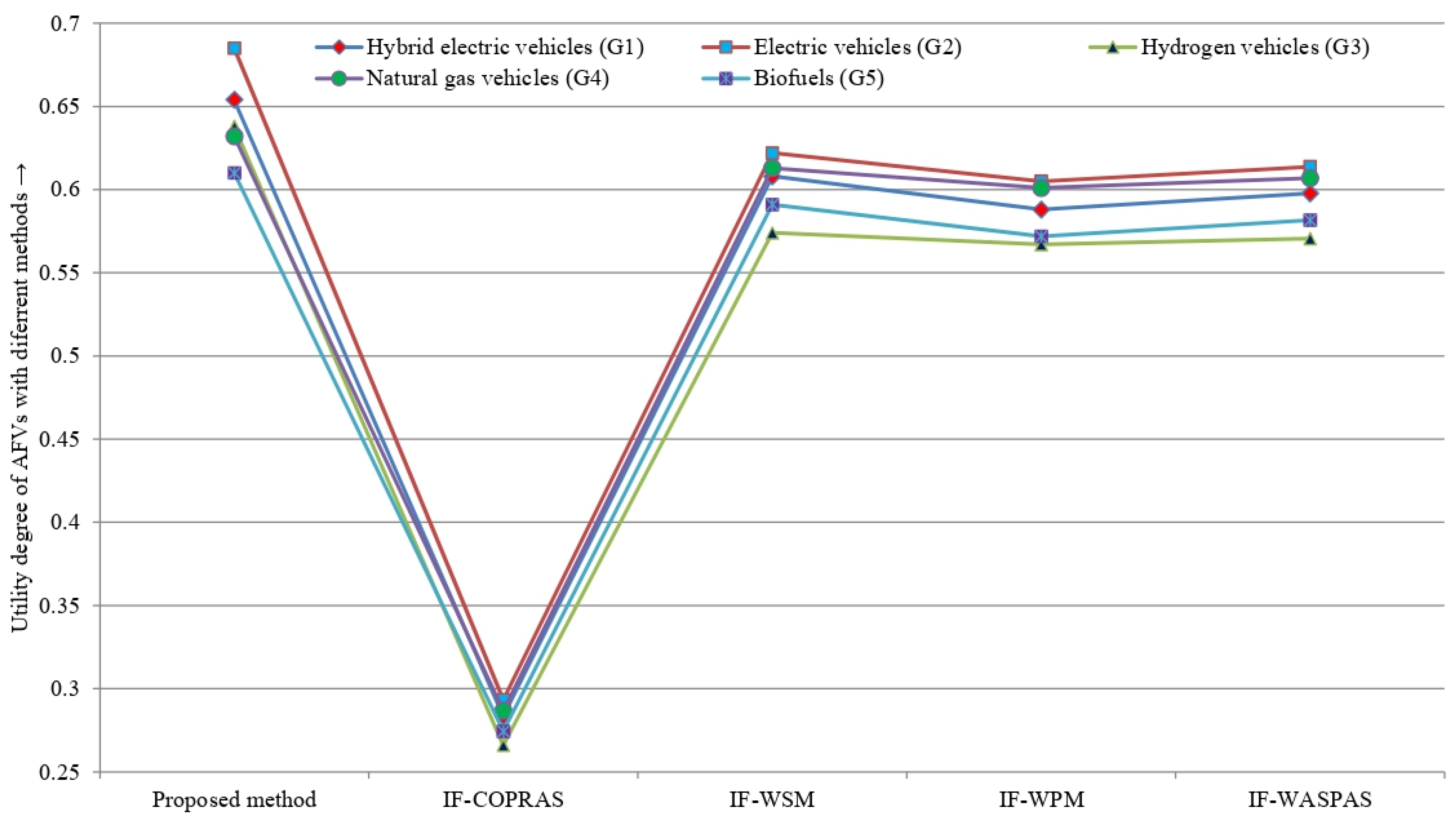
In comparison with existing methods, the benefits of the presented method are discussed as follows (see Figure 3):

• The presented methodology estimates the attribute weights with the use of a combined IF-MEREC-RS process, which achieves more accurate attributes’ weights, while in IF-WASPAS, only the objective weight of criteria is estimated with the use of a similarity measure, and in IF-COPRAS, the weight of criteria is assumed by experts.
• According to the computation procedures of the three methods, we can find the subordinate utility degrees and rank the options by using the IF-DNMA method, which can not only ensure that the selected alternative performs excellently in total, but also avoids the bad performance under each criterion. To this point, the IF-MEREC-RS-DNMA can provide experts with a more robust reference compared with the IF-WASPAS method and IF-COPRAS.
• Aggregation functions used in the IF-MEREC-RS-DNMA model have both the linear and vector normalizations, while the IF-COPRAS model uses vector normalization, and the IF-WASPAS model utilizes the linear normalization. So, the IF-MEREC-RS-DNMA method is more reliable and flexible than extant methods.
• The proposed methodology is applied in the IF-DNMA method to increase the robustness of the fuzzy-DNMA model. Compared to the extant utility based ranking method (namely MULTIMOORA [84], VIKOR [85], TOPSIS [86], ELECTRE [87], COPRAS [81], WASPAS [83], CoCoSo [88], and others), the key benefit of the DNMA approach is that it is considered by two normalization procedures (namely target-based linear and vector normalization). Moreover, DNMA approach gives the DEs to adjust the weight of subordinate models (namely CCM, UCM, and ICM) to reveal their preferences on the “group utility” values and the “individual regret” values of options. Thus, the proposed hybrid DNMA approach is fulfilling the existing gap in the study of AFV assessment.

5.2. Sensitivity Investigation

In this section, we have been changing and investigating the importance of objective and subjective weights for chosen attributes in the presented weighting tool and changing the parameter ϑ of the DNMA method to show the performance of subordinate UDs to the preferences of AFVs. The analyses are carried out by making two cases.

Case I: When utilizing the DNMA method. This subsection shows sensitivity investigation associated with the parameter ϑ. The variation of ϑ is a useful issue helping to evaluate the sensitivity level of the approach, changing from subordinate UDs to the subordinate preferences. In addition, changing the values of ϑ is applied for the sensitivity investigation of the proposed method to the eminence of criteria weights.

Table 15. Ranking results of the IF-MEREC-RS-DNMA method with different values of ϑ.

Θ	G1	G2	G3	G4	G5	Ranking Order
ϑ = 0.0	0.633	0.700	0.533	0.600	0.533	$G_2\succ G_1\succ G_4\succ G_3\succ G_5$
ϑ = 0.1	0.637	0.697	0.568	0.607	0.554	$G_2\succ G_1\succ G_4\succ G_3\succ G_5$
ϑ = 0.2	0.641	0.694	0.591	0.613	0.571	$G_2\succ G_1\succ G_4\succ G_3\succ G_5$
ϑ = 0.3	0.645	0.691	0.609	0.620	0.585	$G_2\succ G_1\succ G_4\succ G_3\succ G_5$
ϑ = 0.4	0.649	0.688	0.624	0.626	0.598	$G_2\succ G_1\succ G_4\succ G_3\succ G_5$
ϑ = 0.5	0.654	0.685	0.638	0.632	0.610	$G_2\succ G_1\succ G_3\succ G_4\succ G_5$
ϑ = 0.6	0.658	0.682	0.651	0.638	0.621	$G_2\succ G_1\succ G_3\succ G_4\succ G_5$
ϑ = 0.7	0.662	0.679	0.662	0.644	0.631	$G_2\succ G_1\approx G_3\succ G_4\succ G_5$
ϑ = 0.8	0.666	0.676	0.673	0.650	0.641	$G_2\succ G_3\succ G_1\succ G_4\succ G_5$
ϑ = 0.9	0.670	0.673	0.683	0.656	0.650	$G_3\succ G_2\succ G_1\succ G_4\succ G_5$
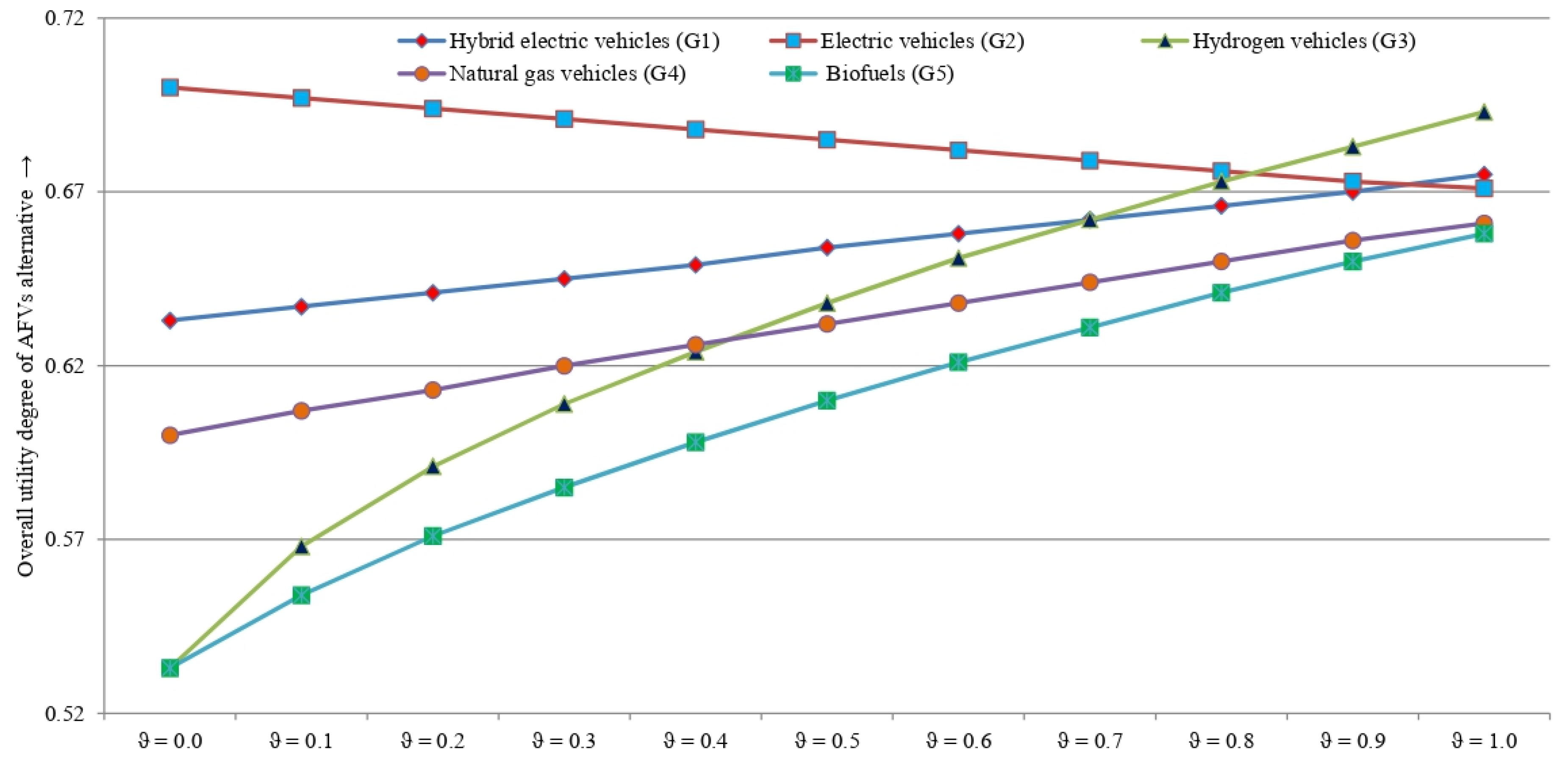
ϑ = 1.0	0.675	0.671	0.693	0.661	0.658	$G_3\succ G_1\succ G_2\succ G_4\succ G_5$

and Figure 4 represent the sensitivity analysis of the AFVs for diverse values of the utility parameter ϑ. Based on the assessments, we obtain the similar preferences $G_2\succ G_1\succ G_4\succ G_3\succ G_5$ for ϑ = 0.0 to ϑ = 0.8, $G_3\succ G_2\succ G_1\succ G_4\succ G_5$ for ϑ = 0.9 and $G_3\succ G_1\succ G_2\succ G_4\succ G_5$ for ϑ = 1.0, which implies G₂ is at the top of the ranking, while the G₅ has the last rank for ϑ = 0.0 to ϑ = 0.8 and the G₃ is at the top of the ranking and G₅ has the last rank for ϑ = 0.9 to ϑ = 1.0. Therefore, it is observable that the developed method possesses adequate stability with numerous parameter values. As shown clearly in Table 15, the developed IF-MEREC-RS-DNMA methodology is capable of generating stable and, at the same time, flexible preference results in a variety of utility parameter. This property is of high importance for MCDM procedures and decision-making reality.

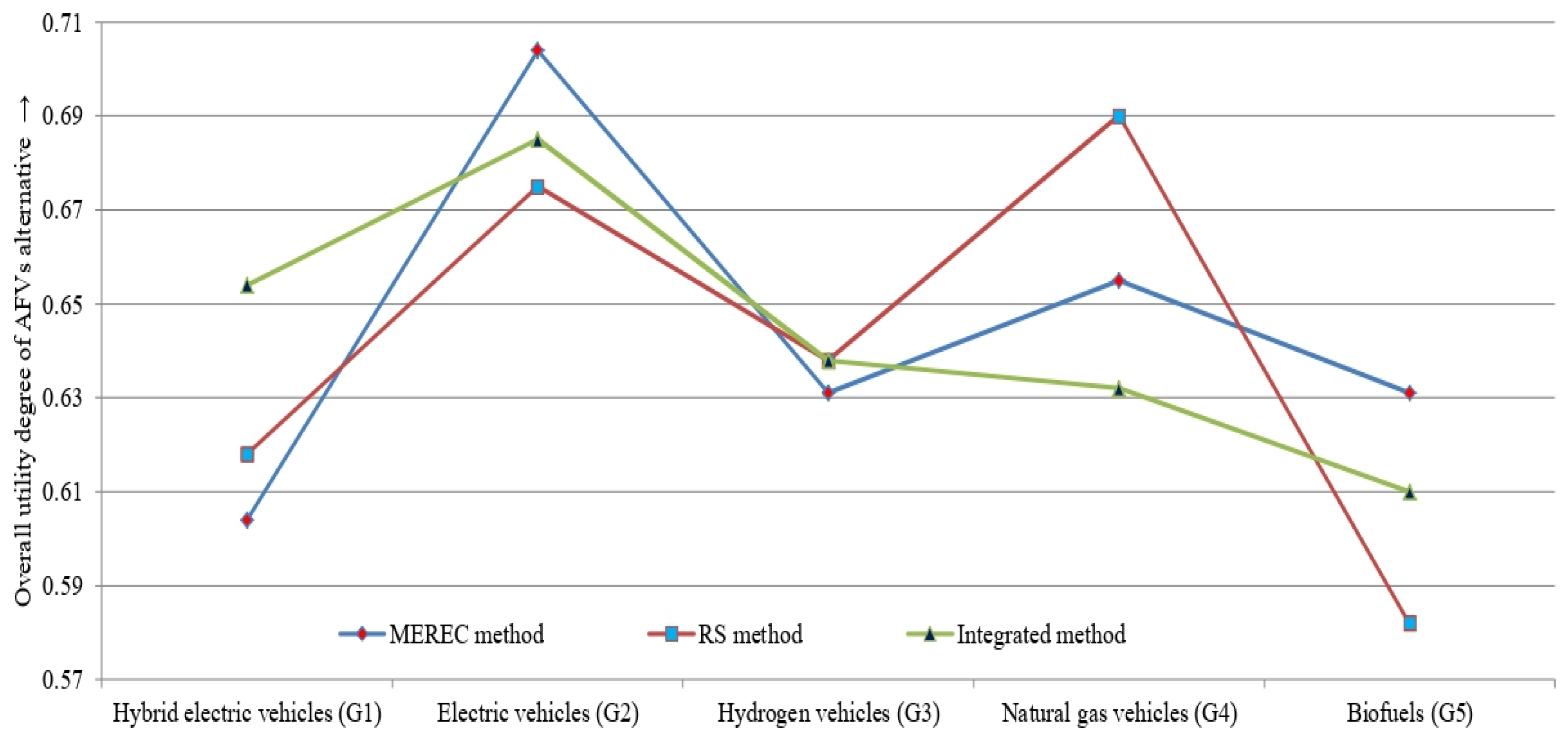
Case II: When introducing a weight-determining approach, the presented weighting tool is registered to offer appropriate weights for considered attributes. Initially, the criteria weights are computed with objective weights using MEREC in the place of combined weights. Thus, the prioritization has been obtained by the objective weighting in place of IF-MEREC-RS weight and presented in

Table 16. Subordinate UD of AFVs over different weighting procedures.

Weighting Procedure	Subordinate UDs of AFVs Options					Ranking Order
	G1	G2	G3	G4	G5
MEREC method	0.604	0.704	0.631	0.655	0.631	$G_2\succ G_4\succ G_3\approx G_5\succ G_1$
RS method	0.618	0.675	0.638	0.690	0.582	$G_4\succ G_2\succ G_3\succ G_1\succ G_5$
Integrated method	0.654	0.685	0.638	0.632	0.610	$G_2\succ G_1\succ G_3\succ G_4\succ G_5$

and Figure 5. Using IF-MEREC, the OUD of AFVs: G₁ = 0.604, G₂ = 0.704, G₃ = 0.631, G₄ = 0.655, and G₅ = 0.631, and the prioritization of the following AFVs:$G_2\succ G_4\succ G_3\approx G_5\succ G_1.$ Applying the RS method, the OUD of the AFVs is as follows: G₁ = 0.618, G₂ = 0.675, G₃ = 0.638, G₄ = 0.690 and G₅ = 0.582 and the prioritization of AFVs as follows:$G_4\succ G_2\succ G_3\succ G_1\succ G_5.$ In the aforementioned discussion, we observe that the diverse parameter values will recover the steadiness of the IF-MEREC-RS-DNMA method.

6. Conclusions

The aim of the study is to propose an innovative MADA methodology with a combination of IF-MEREC-RS and IF-DNMA models for the assessment of candidate AFVs for private fleets. The developed MADA framework offers a better assessment approach to make an effective decision in selecting the most suitable AFV for sustainable transportation. The developed model has been implemented on an illustrative study of an AFV selection problem for a private home healthcare service provider in Chandigarh, India, which confirms its applicability, as well as the effectiveness of the IF-MEREC-RS-DNMA approach. From the sustainable viewpoints, a comprehensive evaluation index system has been made for this case study, which consists of the following five main attributes: economic, social, environmental, technological, and political. In this context, globally existing AFVs for sustainable transportation sector are identified and then prioritized against fifteen different criteria relevant to environmental, economic, technological, social, and political aspects of sustainability. This study contributes to the promotion of sustainable transport and the development of green transport. The proposed model is used to evaluate five alternative fuel vehicles in Chandigarh, India. It is distinguished that electric vehicles (G2), with an overall utility degree of 0.685, hybrid electric vehicles (G1), with an overall utility degree of 0.654, and hydrogen vehicles (G3), with an overall utility degree of 0.638 achieve higher overall performance compared to the other technologies in India. The assessment outcomes prove that electric vehicles can serve as a valuable alternative for decreasing carbon emissions and negative effects on the environment for India. This technology contributes to transportation sector development in less developed areas of the country. The EVs make an important impact on environmental issues since they generate less carbon dioxide than traditional vehicles (gasoline/diesel). The EVs reduce CO, NOx, and SOx gas emissions by 98–100%, 88–100%, and 100%, respectively [5,89]. In another study, Moro and Lonza [90] highlighted that EVs demonstrate average GHG savings of around 50%.

Here, we observe the three main contributions of this study: (1) the development of new intuitionistic fuzzy generalized Dombi aggregation operators that provide the combined information on IFSs; (2) the proposal of a new combination of weighting procedures that enables objective weights using the MEREC and subjective weights using the RS method, and (3) the proposal of a framework which provides a flexible MADA approach for choosing the most sustainable AFV candidate.

It is important to be aware of certain limitations in the developed framework. A practical difficulty is that DEs must be trained with the preference style to properly utilize the flexibility and potential of IFNs. In the following, we present the limitations of the introduced MCDM methodology: (1) In this study, the evaluation index system should include more sustainability criteria, for instance, specific energy consumption, refueling/recharging time, emissions using usage, combustion duration, safety, resale value etc., (2) In realistic circumstances, there is requirement to consider the large number of DEs for assessment of AFV selection, however, we have taken only a set of four DEs, and (3) This work has limitations in dealing with more uncertain decision-making problems because of the constraint condition of the intuitionistic fuzzy set.

Future research studies will try to handle the limitations of this work. Further development of this study is suggested to incorporate other MADM methods such as MARCOS, “operational competitiveness rating (OCRA)” and “multi-attribute ideal real comparative analysis (MAIRCA)” with Archimedean Copula and Aczel–Alsina aggregation operators. Apart from that, other weight-determining methods such as “Level Based Weight Assessment (LBWA)” and FUCOM may be incorporated with DNMA method to improve the MADA process. Moreover, the model presented in this study may be applied to other MADM problems, namely sustainable plastic recycling processes, site selection for electric vehicle charging stations, facility location selection for automotive lithium-ion batteries, and others under different uncertain contexts.

References

1. Onat, N.C.; Noori, M.; Kucukvar, M.; Zhao, Y.; Tatari, O.; Chester, M. Exploring the suitability of electric vehicles in the United States. Energy 2017, 121, 631–642. [Google Scholar] [CrossRef]
2. Ecer, F. A consolidated MCDM framework for performance assessment of battery electric vehicles based on ranking strategies. Renew. Sustain. Energy Rev. 2021, 143, 110916. [Google Scholar] [CrossRef]
3. Demeulenaere, X. The use of automotive fleets to support the diffusion of alternative fuel vehicles: A rapid evidence assessment of barriers and decision mechanisms. Res. Transp. Econ. 2019, 76, 100738. [Google Scholar] [CrossRef]
4. Bartolozzi, I.; Rizzi, F.; Frey, M. Comparison between hydrogen and electric vehicles by life cycle assessment: A case study in Tuscany, Italy. Appl. Energy 2013, 101, 103–111. [Google Scholar] [CrossRef]
5. Pamucar, D.; Ecer, F.; Deveci, M. Assessment of alternative fuel vehicles for sustainable road transportation of United States using integrated fuzzy FUCOM and neutrosophic fuzzy MARCOS methodology. Sci. Total Environ. 2021, 788, 147763. [Google Scholar] [CrossRef] [PubMed]
6. Van Mierlo, J.; Messagie, M.; Rangaraju, S. Comparative environmental assessment of alternative fueled vehicles using a life cycle assessment. Transp. Res. Procedia 2017, 25, 3435–3445. [Google Scholar] [CrossRef]
7. Bicer, Y.; Dincer, I. Life cycle environmental impact assessments and comparisons of alternative fuels for clean vehicles. Resour. Conserv. Recycl. 2018, 132, 141–157. [Google Scholar] [CrossRef]
8. Chang, D.-S.; Chen, S.-H.; Hsu, C.-W.; Hu, A.H.; Tzeng, G.-H. Evaluation Framework for Alternative Fuel Vehicles: Sustainable Development Perspective. Sustainability 2015, 7, 11570–11594. [Google Scholar] [CrossRef] [Green Version]
9. Ghosh, A. Possibilities and Challenges for the Inclusion of the Electric Vehicle (EV) to Reduce the Carbon Footprint in the Transport Sector: A Review. Energies 2020, 13, 2602. [Google Scholar] [CrossRef]
10. Kene, R.; Olwal, T.; van Wyk, B.J. Sustainable Electric Vehicle Transportation. Sustainability 2021, 13, 12379. [Google Scholar] [CrossRef]
11. Offer, G.J.; Howey, D.; Contestabile, M.; Clague, R.; Brandon, N.P. Comparative analysis of battery electric, hydrogen fuel cell and hybrid vehicles in a future sustainable road transport system. Energy Policy 2010, 38, 24–29. [Google Scholar] [CrossRef] [Green Version]
12. Faria, R.; Marques, P.; Moura, P.; Freire, F.; Delgado, J.; de Almeida, A.T. Impact of the electricity mix and use profile in the life-cycle assessment of electric vehicles. Renew. Sustain. Energy Rev. 2013, 24, 271–287. [Google Scholar] [CrossRef]
13. Krishnan, V.; Gonzalez-Marciaga, L.; McCalley, J. A planning model to assess hydrogen as an alternative fuel for national light-duty vehicle portfolio. Energy 2014, 73, 943–957. [Google Scholar] [CrossRef]
14. Wu, D.; Aliprantis, D.C. Modeling light-duty plug-in electric vehicles for national energy and transportation planning. Energy Policy 2013, 63, 419–432. [Google Scholar] [CrossRef]
15. Liu, J.; Khattak, A.; Wang, X. The role of alternative fuel vehicles: Using behavioral and sensor data to model hierarchies in travel. Transp. Res. Part C Emerg. Technol. 2015, 55, 379–392. [Google Scholar] [CrossRef]
16. Yavuz, M.; Çapar, İ. Alternative-Fuel Vehicle Adoption in Service Fleets: Impact Evaluation Through Optimization Modeling. Transp. Sci. 2016, 51, 480–493. [Google Scholar] [CrossRef]
17. Mizik, T. Sustainable fuels in private transportation—Present and future potential. In Clean Fuels for Mobility. Energy, Environment, and Sustainability; Di Blasio, G., Agarwal, A.K., Belgiorno, G., Shukla, P.C., Eds.; Springer: Singapore, 2022. [Google Scholar] [CrossRef]
18. Onat, N.C. How to compare sustainability impacts of alternative fuel Vehicles? Transp. Res. Part D Transp. Environ. 2022, 102, 103129. [Google Scholar] [CrossRef]
19. Loo, D.L.; Teoh, Y.H.; How, H.G.; Teh, J.S.; Andrei, L.C.; Starčević, S.; Sher, F. Applications Characteristics of Different Biodiesel Blends in Modern Vehicles Engines: A Review. Sustainability 2021, 13, 9677. [Google Scholar] [CrossRef]
20. Peksen, M. Hydrogen Technology towards the Solution of Environment-Friendly New Energy Vehicles. Energies 2021, 14, 4892. [Google Scholar] [CrossRef]
21. Betancourt-Torcat, A.; Charry-Sanchez, J.; Almansoori, A.; Alkatheri, M.; Flett, P.; Elkamel, A. An integrated electric vehicle network planning with economic and ecological assessment: Application to the incipient middle Eastern market in transition towards sustainability. J. Clean. Prod. 2021, 302, 126980. [Google Scholar] [CrossRef]
22. Sinha, P.; Brophy, B. Life cycle assessment of renewable hydrogen for fuel cell passenger vehicles in California. Sustain. Energy Technol. Assess. 2021, 45, 101188. [Google Scholar] [CrossRef]
23. Antonini, C.; Treyer, K.; Moioli, E.; Bauer, C.; Tilman, J.S.; Mazzotti, M. Hydrogen from wood gasification with CCS—A techno-environmental analysis of production and use as transport fuel. Sustain. Energy Fuels 2021, 5, 2602–2621. [Google Scholar] [CrossRef]
24. Gharib, M.R. Comparison of robust optimal QFT controller with TFC and MFC controller in a multi-input multi-output system. Rep. Mech. Eng. 2020, 1, 151–161. [Google Scholar] [CrossRef]
25. Zadeh, L.A. Fuzzy sets. Inf. Control 1965, 8, 338–353. [Google Scholar] [CrossRef] [Green Version]
26. Mendel, J.M. On computing the similarity of trapezoidal fuzzy sets using an Automated Area Method. Inf. Sci. 2022, 589, 716–737. [Google Scholar] [CrossRef]
27. Ma, Z.; Yan, L. Data modeling and querying with fuzzy sets: A systematic survey. Fuzzy Sets Syst. 2022; in press. [Google Scholar] [CrossRef]
28. Oliveira, L.D.S.; Argou, A.; Dilli, R.; Yamin, A.; Reiser, R.; Bedregal, B. Exploring fuzzy set consensus analysis in IoT resource ranking. Eng. Appl. Artif. Intell. 2022, 109, 104617. [Google Scholar] [CrossRef]
29. Atanassov, K.T. Intuitionistic fuzzy sets. Fuzzy Sets Syst. 1986, 20, 87–96. [Google Scholar] [CrossRef]
30. Alcantud, J.C.R.; Khameneh, A.Z.; Kilicman, A. Aggregation of infinite chains of intuitionistic fuzzy sets and their application to choices with temporal intuitionistic fuzzy information. Inf. Sci. 2020, 514, 106–117. [Google Scholar] [CrossRef]
31. Hao, Z.; Xu, Z.; Zhao, H.; Zhang, R. The context-based distance measure for intuitionistic fuzzy set with application in marine energy transportation route decision making. Appl. Soft Comput. 2021, 101, 107044. [Google Scholar] [CrossRef]
32. Pan, L.; Deng, Y. A novel similarity measure in intuitionistic fuzzy sets and its applications. Eng. Appl. Artif. Intell. 2022, 107, 104512. [Google Scholar] [CrossRef]
33. Žižović, M.; Pamučar, D. New model for determining criteria weights: Level based weight assessment (LBWA) model. Decis. Mak. Appl. Manag. Eng. 2019, 2, 126–137. [Google Scholar] [CrossRef]
34. Şahin, M. A comprehensive analysis of weighting and multicriteria methods in the context of sustainable energy. Int. J. Environ. Sci. Technol. 2021, 18, 1591–1616. [Google Scholar] [CrossRef] [PubMed]
35. Stanujkic, D.; Karabaševic, D.; Popovic, G.; Stanimirovic, P.S.; Saracevic, M.; Smarandache, F.; Katsikis, V.N.; Ulutas, A. A new grey approach for using SWARA and PIPRECIA methods in a group decision-making environment. Mathematics 2021, 9, 1554. [Google Scholar] [CrossRef]
36. Keshavarz-Ghorabaee, M.; Amiri, M.; Zavadskas, E.K.; Turskis, Z.; Antucheviciene, J. Determination of objective weights using a new method based on the removal effects of criteria (MEREC). Symmetry 2021, 13, 525. [Google Scholar] [CrossRef]
37. Rani, P.; Mishra, A.R.; Saha, A.; Hezam, I.M.; Pamucar, D. Fermatean Fuzzy Heronian Mean Operators and MEREC-Based Additive Ratio Assessment Method: An Application to Food Waste Treatment Technology Selection. Int. J. Intell. Syst. 2021, 37, 2612–2647. [Google Scholar] [CrossRef]
38. Stillwell, W.G.; Seaver, D.A.; Edwards, W. A comparison of weight approximation techniques in multi-attribute utility decision making. Organ. Behav. Hum. Perform. 1981, 28, 62–77. [Google Scholar] [CrossRef]
39. Liao, H.; Wu, X. DNMA: A double normalization-based multiple aggregation method for multi-expert multi-criteria decision making. Omega 2020, 94, 102058. [Google Scholar] [CrossRef]
40. He, J.; Huang, Z.; Mishra, A.R.; Alrasheedi, M. Developing a new framework for conceptualizing the emerging sustainable community-based tourism using an extended interval-valued Pythagorean fuzzy SWARA-MULTIMOORA. Technol. Forecast. Soc. Change 2021, 171, 120955. [Google Scholar] [CrossRef]
41. Domingues, A.R.; Marques, P.; Garcia, R.; Freire, F.; Dias, L.C. Applying Multi-Criteria Decision Analysis to the Life-Cycle Assessment of vehicles. J. Clean. Prod. 2015, 107, 749–759. [Google Scholar] [CrossRef] [Green Version]
42. Yavuz, M.; Oztaysi, B.; Onar, S.C.; Kahraman, C. Multi-criteria evaluation of alternative-fuel vehicles via a hierarchical hesitant fuzzy linguistic model. Expert Syst. Appl. 2015, 42, 2835–2848. [Google Scholar] [CrossRef]
43. Oztaysi, B.; Onar, S.C.; Kahraman, C.; Yavuz, M. Multi-criteria alternative-fuel technology selection using interval-valued intuitionistic fuzzy sets. Transp. Res. Part D Transp. Environ. 2017, 53, 128–148. [Google Scholar] [CrossRef]
44. Liang, H.; Ren, J.; Lin, R.; Liu, Y. Alternative-fuel based vehicles for sustainable transportation: A fuzzy group decision supporting framework for sustainability prioritization. Technol. Forecast. Soc. Chang. 2019, 140, 33–43. [Google Scholar] [CrossRef]
45. Shao, Y.; Dessouky, M. A routing model and solution approach for alternative fuel vehicles with consideration of the fixed fueling time. Comput. Ind. Eng. 2020, 142, 106364. [Google Scholar] [CrossRef]
46. Rani, P.; Mishra, A.R. Multi-Criteria Weighted Aggregated Sum Product Assessment Framework for Fuel Technology Selection using q-Rung Orthopair Fuzzy Sets. Sustain. Prod. Consum. 2020, 24, 90–104. [Google Scholar] [CrossRef]
47. Mishra, A.R.; Rani, P. Shapley divergence measures with VIKOR method for multi-attribute decision making problems. Neural Comput. Appl. 2019, 31, 1299–1316. [Google Scholar] [CrossRef]
48. Abdullah, L.; Ong, Z.; Rahim, N. An Intuitionistic Fuzzy Decision-Making for Developing Cause and Effect Criteria of Subcontractors Selection. Int. J. Comput. Intell. Syst. 2021, 14, 991–1002. [Google Scholar] [CrossRef]
49. Fei, L.; Feng, Y. Intuitionistic fuzzy decision-making in the framework of Dempster–Shafer structures. Int. J. Intell. Syst. 2021, 36, 5419–5448. [Google Scholar] [CrossRef]
50. Jana, C.; Muhiuddin, G.; Pal, M.; Al-Kadi, D. Intuitionistic Fuzzy Dombi Hybrid Decision-Making Method and Their Applications to Enterprise Financial Performance Evaluation. Math. Probl. Eng. 2021, 2021, 3218133. [Google Scholar] [CrossRef]
51. Zhou, L.-P.; Wan, S.-P.; Dong, J.-Y. A Fermatean Fuzzy ELECTRE Method for Multi-Criteria Group Decision-Making. Informatica 2021, 33, 181–224. [Google Scholar] [CrossRef]
52. Molla, M.U.; Giri, B.C.; Biswas, P. Extended PROMETHEE method with Pythagorean fuzzy sets for medical diagnosis problems. Soft Comput. 2021, 25, 4503–4512. [Google Scholar] [CrossRef]
53. Kutlu, G.F.; Kahraman, C. Spherical fuzzy sets and spherical fuzzy TOPSIS method. J. Intell. Fuzzy Syst. 2019, 36, 337–352. [Google Scholar] [CrossRef]
54. Cheng, S.; Jianfu, S.; Alrasheedi, M.; Saeidi, P.; Mishra, A.R.; Rani, P. A new extended VIKOR approach using q-rung orthopair fuzzy sets for sustainable enterprise risk management assessment in manufacturing small and medium-sized enterprises. Int. J. Fuzzy Syst. 2021, 23, 1347–1369. [Google Scholar] [CrossRef]
55. Mahmood, T.; Warraich, M.S.; Ali, Z.; Pamucar, D. Generalized MULTIMOORA method and Dombi prioritized weighted aggregation operators based on T-spherical fuzzy sets and their applications. Int. J. Fuzzy Syst. 2021, 36, 4659–4692. [Google Scholar] [CrossRef]
56. Nie, S.; Liao, H.; Wu, X.; Tang, M.; Al-Barakati, A. Hesitant fuzzy linguistic DNMA method with cardinal consensus reaching process for shopping mall location selection. Int. J. Strateg. Prop. Manag. 2019, 23, 420–434. [Google Scholar] [CrossRef] [Green Version]
57. Lai, H.; Liao, H.; Šaparauskas, J.; Banaitis, A.; Ferreira, F.A.F.; Al-Barakati, A. Sustainable cloud service provider development by a Z-number-based DNMA method with gini-coeffcient-based weight determination. Sustainability 2020, 12, 3410. [Google Scholar] [CrossRef] [Green Version]
58. Lai, H.; Liao, H. A multi-criteria decision making method based on DNMA and CRITIC with linguistic D numbers for blockchain platform evaluation. Eng. Appl. Artif. Intell. 2021, 101, 104200. [Google Scholar] [CrossRef]
59. Wang, L.; Rani, P. Sustainable supply chains under risk in the manufacturing firms: An extended double normalization-based multiple aggregation approach under an intuitionistic fuzzy environment. J. Enterp. Inf. Manag. 2021. [Google Scholar] [CrossRef]
60. Xu, Z.S. Intuitionistic fuzzy aggregation operators. IEEE Trans. Fuzzy Syst. 2007, 15, 1179–1187. [Google Scholar]
61. Xu, G.L.; Wan, S.P.; Xie, X.L. A Selection Method Based on MAGDM with Interval-Valued Intuitionistic Fuzzy Sets. Math. Probl. Eng. 2015, 2015, 791204. [Google Scholar] [CrossRef] [Green Version]
62. Dombi, J. The generalized dombi operator family and the multiplicative utility function. In Soft Computing Based Modeling in Intelligent Systems. Studies in Computational Intelligence; Balas, V.E., Fodor, J., Várkonyi-Kóczy, A.R., Eds.; Springer: Berlin/Heidelberg, Germany, 2009; p. 196. [Google Scholar] [CrossRef]
63. Narayanamoorthy, S.; Annapoorani, V.; Kang, D.; Baleanu, D.; Jeon, J.; Kureethara, J.V.; Ramya, L. A novel assessment of bio-medical waste disposal methods using integrating weighting approach and hesitant fuzzy MOOSRA. J. Clean. Prod. 2020, 275, 122587. [Google Scholar] [CrossRef]
64. Chen, S.J.; Hwang, C.L. Fuzzy Multiple Attribute Decision Making: Methods and Applications; Springer: Berlin/Hedelberg, Germany, 1992. [Google Scholar]
65. Rani, P.; Mishra, A.R.; Saha, A.; Pamucar, D. Pythagorean fuzzy weighted discrimination-based approximation approach to the assessment of sustainable bioenergy technologies for agricultural residues. Int. J. Intell. Syst. 2021, 36, 2964–2990. [Google Scholar] [CrossRef]
66. Maimoun, M.; Madani, K.; Reinhart, D. Multi-levelmulti-criteria analysis of alternative fuels for waste collection vehicles in the United States. Sci. Total Environ. 2016, 550, 349–361. [Google Scholar] [CrossRef] [PubMed] [Green Version]
67. Mohamadabadi, H.S.; Tichkowsky, G.; Kumar, A. Development of a multi-criteria assessment model for ranking of renewable and non-renewable transportation fuel vehicles. Energy 2009, 34, 112–125. [Google Scholar] [CrossRef]
68. Egner, F.; Trosvik, L. Electric vehicle adoption in Sweden and the impact of local policy instruments. Energy Policy 2018, 121, 584–596. [Google Scholar] [CrossRef] [Green Version]
69. Sovacool, B.K.; Kester, J.; Noel, L.; de Rubens, G.Z. The demographics of decarbonizing transport: The influence of gender, education, occupation, age, and household size on electric mobility preferences in the Nordic region. Glob. Environ. Chang. 2018, 52, 86–100. [Google Scholar] [CrossRef]
70. Lin, C.W.; Chen, S.H.; Tzeng, G.H. Constructing a cognition map of alternative fuel vehicles using the DEMATEL method. J. Multi-Criteria Decis. Anal. 2009, 16, 5–19. [Google Scholar] [CrossRef]
71. Tsita, K.G.; Pilavachi, P.A. Evaluation of alternative fuels for the Greek road transport sector using the analytic hierarchy process. Energy Policy 2012, 48, 677–686. [Google Scholar] [CrossRef]
72. Xu, M.; Meng, Q.; Liu, Y. Public’s perception of adopting electric vehicles: A case study of Singapore. J. East. Asia Soc. Transp. Stud. 2017, 12, 285–298. [Google Scholar]
73. Tzeng, G.H.; Lin, C.W.; Opricovic, S. Multi-criteria analysis of alternative-fuel buses for public transportation. Energy Policy 2005, 33, 1373–1383. [Google Scholar] [CrossRef]
74. Sehatpour, M.H.; Kazemi, A.; Sehatpour, H.E. Evaluation of alternative fuels for light-duty vehicles in Iran using a multi-criteria approach. Renew. Sustain. Energ. Rev. 2017, 72, 295–310. [Google Scholar] [CrossRef]
75. Daramy-Williams, E.; Anable, J.; Grant-Muller, S. A systematic review of the evidence on plug-in electric vehicle user experience. Transp. Res. Part D Transp. Environ. 2019, 71, 22–36. [Google Scholar] [CrossRef] [Green Version]
76. Al-Alawi, B.M.; Bradley, T.H. Total cost of ownership, payback, and consumer preference modeling of plug-in hybrid electric vehicles. Appl. Energy 2013, 103, 488–506. [Google Scholar] [CrossRef]
77. Swart, D.J.; Bekker, A.; Bienert, J. The subjective dimensions of sound quality of standard production electric vehicles. Appl. Acoust. 2018, 129, 354–364. [Google Scholar] [CrossRef]
78. Jena, R. An empirical case study on Indian consumers’ sentiment towards electric vehicles: A big data analytics approach. Ind. Mark. Manag. 2020, 90, 605–616. [Google Scholar] [CrossRef]
79. Okada, T.; Tamaki, T.; Managi, S. Effect of environmental awareness on purchase intention and satisfaction pertaining to electric vehicles in Japan. Transp. Res. Part D Transp. Environ. 2019, 67, 503–513. [Google Scholar] [CrossRef]
80. Brey, J.J.; Contreras, I.; Carazo, A.F.; Brey, R.; Hernández-Díaz, A.G.; Castro, A. Evaluation of automobiles with alternative fuels utilizing multicriteria techniques. J. Power Sources 2007, 169, 213–219. [Google Scholar] [CrossRef]
81. Kumari, R.; Mishra, A.R. Multi-criteria COPRAS method based on parametric measures for intuitionistic fuzzy sets: Application of green supplier selection. Iran. J. Sci. Technol. Trans. Electr. Eng. 2020, 44, 1645–1662. [Google Scholar] [CrossRef]
82. Gitinavard, H.; Shirazi, M.A. An extended intuitionistic fuzzy modified group complex proportional assessment approach. J. Ind. Syst. Eng. 2018, 11, 229–246. [Google Scholar]
83. Mishra, A.R.; Singh, R.K.; Motwani, D. Multi-criteria assessment of cellular mobile telephone service providers using intuitionistic fuzzy WASPAS method with similarity measures. Granul. Comput. 2019, 4, 511–529. [Google Scholar] [CrossRef]
84. Mishra, A.R.; Saha, A.; Rani, P.; Hezam, I.M.; Shrivastava, R.; Smarandache, F. An Integrated Decision Support Framework Using Single-Valued-MEREC-MULTIMOORA for Low Carbon Tourism Strategy Assessment. IEEE Access 2022, 10, 24411–24432. [Google Scholar] [CrossRef]
85. Mishra, A.R.; Rani, P.; Prajapati, R.S. Multi-criteria weighted aggregated sum product assessment method for sustainable biomass crop selection problem using single-valued neutrosophic sets. Appl. Soft Comput. 2021, 113, 108038. [Google Scholar] [CrossRef]
86. Mishra, A.R.; Rani, P.; Jain, D. Information measures based TOPSIS method for multicriteria decision making problem in intuitionistic fuzzy environment. Iran. J. Fuzzy Syst. 2017, 14, 41–63. [Google Scholar] [CrossRef]
87. Mishra, A.R.; Singh, R.K.; Motwani, D. Intuitionistic fuzzy divergence measure-based ELECTRE method for performance of cellular mobile telephone service providers. Neural Comput. Appl. 2020, 32, 3901–3921. [Google Scholar] [CrossRef]
88. Mishra, A.R.; Rani, P.; Saha, A.; Hezam, I.M.; Pamucar, D.; Marinovic, M.; Pandey, K. Assessing the Adaptation of Internet of Things (IoT) Barriers for Smart Cities’ Waste Management Using Fermatean Fuzzy Combined Compromise Solution Approach. IEEE Access 2022, 10, 37109–37130. [Google Scholar] [CrossRef]
89. Kazimi, C. Evaluating the environmental impact of alternative-fuel vehicles. J. Environ. Econ. Manag. 1997, 33, 163–185. [Google Scholar] [CrossRef]
90. Moro, A.; Lonza, L. Electricity carbon intensity in European Member States: Impacts on GHG emissions of electric vehicles. Transp. Res. Part D Transp. Environ. 2018, 64, 5–14. [Google Scholar] [CrossRef]
Figure 1. Flowchart of the proposed methodology.
Sustainability 14 05463 g001
Figure 2. Weight of criteria for AFVs selection using IF-MEREC-RS method.
Sustainability 14 05463 g002
Figure 3. Ranking order of AFVs option with different approaches.
Sustainability 14 05463 g003
Figure 4. Ranking order of AFVs option with different approaches.
Sustainability 14 05463 g004
Figure 5. Sensitivity analysis of AFVs with different weighting procedures.
Sustainability 14 05463 g005