Article

Image Classification Method Based on Improved Deep Convolutional Neural Networks for the Magnetic Flux Leakage (MFL) Signal of Girth Welds in Long-Distance Pipelines

1
College of Safety and Ocean Engineering, China University of Petroleum (Beijing), Beijing 102200, China
2
PipeChina Company, Beijing 100020, China
*
Author to whom correspondence should be addressed.
Sustainability 2022, 14(19), 12102; https://doi.org/10.3390/su141912102
Submission received: 27 July 2022 / Revised: 18 September 2022 / Accepted: 22 September 2022 / Published: 24 September 2022

Abstract

:
Girth weld defects in long-distance oil and gas pipelines are one of the main causes of pipeline leakage failure and serious accidents. Magnetic flux leakage (MFL) is one of the most widely used inline inspection methods for long-distance pipelines. However, it is impossible to determine the type of girth weld defect via traditional manual analysis due to the complexity of the MFL signal. Therefore, an automatic image classification method based on deep convolutional neural networks was proposed to effectively classify girth weld defects via MFL signals. Firstly, the image data set of girth welds MFL signal was established with the radiographic testing results as labels. Then, the deep convolutional generative adversarial network (DCGAN) data enhancement algorithm was proposed to enhance the data set, and the residual network (ResNet-50) was proposed to address the challenge presented by the automatic classification of the image sets. The data set after data enhancement was randomly selected to train and test the improved residual network (ResNet-50), with the ten validation results exhibiting an accuracy of over 80%. The results indicated that the improved network model displayed a strong generalization ability and robustness and could achieve a more accurate MFL image classification of the pipeline girth welds.

1. Introduction

Long-distance oil and gas pipelines represent the primary routes for oil and gas transportation, playing a vital role in economic development [1,2]. Recent years have seen frequent pipeline leakage failures caused by girth weld cracking in oil and gas pipelines, resulting in significant economic losses, environmental pollution, and even casualties. The timely discovery and repair of girth weld defects can effectively avoid accidents and ensure pipeline safety [3,4]. Since long-distance oil and gas pipelines are installed underground, pipeline operators must perform the following procedure to check for girth weld defects: (1) Excavate the pipeline. (2) Strip the pipeline anti-corrosion layer. (3) Polish the girth weld to be tested. (4) Conduct non-destructive testing on the girth welds to check for defects. Radiographic testing is typically used in gas pipelines, while the defects can include circular defects, strip defects, incomplete fusion, incomplete penetration, crack, pits, and undercuts. According to the type of defect and other factors, the pipeline operators decide how to deal with them, and make sure the pipeline girth welds avoid cracking. However, there is a risk of pipeline damage during excavation, and subsequent non-destructive testing takes a long time. The number of girth welds in each pipeline is extensive, with more than 8000 girth welds per 100 km, making it impossible to excavate all of them. MFL in-line inspection is the most widely used trenchless in-line inspection method for long-distance oil and gas pipelines, and the obtained MFL in-line inspection signals can represent the information of the pipeline body and all the girth welds. However, it is impossible to determine the girth weld defect type via traditional manual analysis due to the complexity of the MFL signal. Therefore, it is necessary to intelligently recognize and classify the MFL in-line inspection images of the girth weld. The type of weld defects can be known without excavation using this method, which can help judge whether the girth weld has cracking risk in advance. This can assist pipeline operators in the safety management of girth weld. Therefore, this work is critical for long-distance oil and gas pipeline safety management.
A convolutional neural network (CNN) can extract higher-dimensional features and prevent the limitation presented by manual feature recognition and performance in image processing and is widely used in industry, agriculture, medicine, food, and other fields [5,6,7,8,9,10,11,12,13,14,15]. Especially in the field of face recognition, audio retrieval, and clinical diagnostic features of cardiovascular diseases, in-depth research is abundant; the classification and recognition performance of the international open data set of the above areas is excellent. For example, the recognition accuracy of the Labeled Faces in the Wild (LFW) database is 97.35%, which is comparable to the recognition accuracy of human eyes of 97.53% [16]; the error rate of the standard TIMIT speech database is reduced by 10% compared to other neural network models [17,18] and the accuracy of ECG classification in the MIT-BIH database, an internationally recognized arrhythmia database, was 99.2% [19]. CNNs have three advantages: weight sharing, multi-layer structure and pooling operation. Weight sharing reduces the training parameters in the network, decreases the complexity of the network model, and reduces overfitting, consequently improving the generalization ability of the model. CNNs with a deep structure have strong learning abilities and can handle more complex problems. Pooling operations reduce the number of neurons of the network, improving its robustness. Based on all these characters of CNNs and complexity of the girth weld image, a deep convolutional neural network is selected for image classification in this paper.
However, minimal research is currently available regarding the classification of girth weld defect images using a deep convolutional neural network. Yang et al. [20] proposed a magnetic flux leakage (MFL) image classification method based on sparse auto-coding to classify girth weld and spiral weld images. Wang et al. [21] used the Hidden Markov Random Field (HMRF) model and the Bayesian model to perform cluster analyses of pipeline corrosion defects. Chen et al. [22] used a radial basis neural network as a prediction model for defects detected by MFL in-line inspection and combined it with the gradient descent method to update the defect profile. Khodahari [23] identified pipeline body defects in MFL in-line inspection images via machine learning. The reasons why minimal research is available are: (1) It is challenging to obtain data set labels. After the excavation of the girth weld, nondestructive testing determined the label of the girth weld MFL signal. According to the first paragraph description, the excavation and detection of the girth weld is a time-consuming and labor-intensive process that requires a significant amount of workforce and material resources to complete. (2) It is difficult to guarantee the number of data sets. The data set is limited to selecting the MFL signal images of the girth weld within the same in-line inspection segment. Under the influence of medium velocity and more, the set parameters of the MFL in-line inspection of different segments are different, so the girth-weld MFL signal images in different detection sections cannot be used in the same data set. As for the data set for this paper, the girth weld MFL signal images in a natural gas pipeline section are selected. In this segment, girth weld defects caused severe accidents. Therefore, the pipeline operator conducted over 1000 girth weld excavations and obtained the data set. This data set has not been made public by the pipeline operator.
CNN involves the AlexNet model, the GoogleNet model, the VGG model, the ResNet model, and many more, all of which performed exceptionally well in the ImageNet competition. Krizhevsky et al. [24] used the AlexNet model, containing five convolutional layers and two fully connected layers in the LSVRC-12 image classification competition. The model achieved a good classification effect. However, this model depth was relatively shallow compared to other network models. Szegedy et al. [25] proposed a GoogLeNet model with over 20 layers and three types of convolution operations (1 × 1, 3 × 3, and 5 × 5). This structure won first place in the “Specified Data” category of the LSVRC-14 image classification competition for its improved utilization of computing resources and increased accuracy. Simonyan et al. [26] replaced a convolution layer with a large convolution kernel with multiple convolution layers with small convolution kernels (e.g., three convolution layers with all sizes of 3 × 3 convolution kernels replaced one convolution layer with 7 × 7 convolution kernels). The VGG model depth increased while parameter count was reduced by increasing the convolution layers of 3 × 3 convolution kernels. When the number of weight layers reaches 16–19, the model performance can be effectively improved. This model won second place at the LSVRC-14 image classification competition in the “Specified Data” category. Due to the extensive depth and complex structure of the VGG and GoogLeNet networks, the training period is lengthy, and VGG must repeatedly adjust the network parameters. Deep network models are prone to degradation, which means that as the network depth increases, so does training error, causing the network accuracy to reach saturation and then rapidly decline. In 2015, K.He et al. proposed Residual Network (ResNet) to address the degradation issue [27]. The model features cross-layer joining, in which the input is passed across layers and added to the convolution result through shortcut connections. The model has only one pooling layer, which is connected to the final convolutional layer. These features enable the ResNet underlying network to be fully trained, which improves accuracy significantly as depth increases. This model won first place at the LSVRC-15 image classification competition. The network structures of the AlexNet and VGG models are both linear, and their inputs are transmitted directly from the first convolutional layer to the final layer along a single path, making it challenging to optimize the underlying network parameters [28]. GoogleNet augments multiple middle tiers with supervisory signals. ResNet, in contrast to these other three network models, uses shortcut connections technology to pass the input across layers to the bottom layer, greatly simplifying the training process for deep network models and improving their classification accuracy. Therefore, this paper improves the deep residual network (ResNet-50) image classification model to classify MFL in-line inspection images of girth welds.
The data set in this paper contains over 1000 images of girth welds MFL signals, displaying few data and unbalanced classification, and these easily cause unstable network training, over-fitting, and poor generalization ability [29,30]. Jun et al. [31] used tailoring to increase the data set size and achieve category balance. Ukil et al. [32] combined oversampling with semi-supervised feedback control to obtain an intelligent enhancement algorithm. Shaker et al. [29] used a generative adversarial network (GAN) for data enhancement, confirming that this method was superior to other traditional data enhancement techniques. However, the GAN presents challenges, such as pattern collapse, discriminator victory, instability, and slow convergence [33,34]. Recent studies have shown that GAN with gradient punishment can overcome these challenges and reduce training time [35,36,37]. This paper applies the gradient descent method to the GAN to optimize the network performance and enhance the data sets, which addresses the challenge of few data in the original data set. In order to focus on effective key features and improve the recognition rate and robustness of the classification model, CBAM is embedded into the ResNet-50 network. The improved ResNet-50 network is trained with the enhanced data set, displaying classification accuracy of over 80% with the ten validation results. The results show that the improved model exhibits a strong generalization ability and can accurately classify pipeline girth weld MFL images.

2. Principle

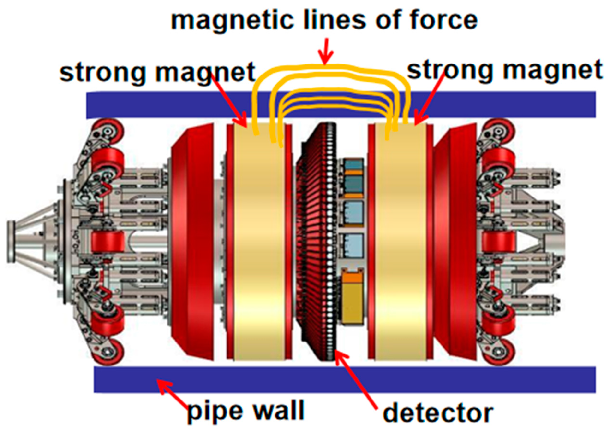
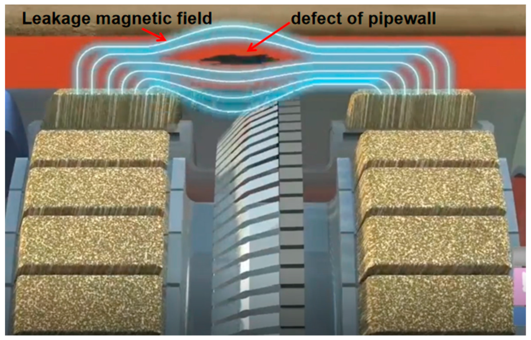
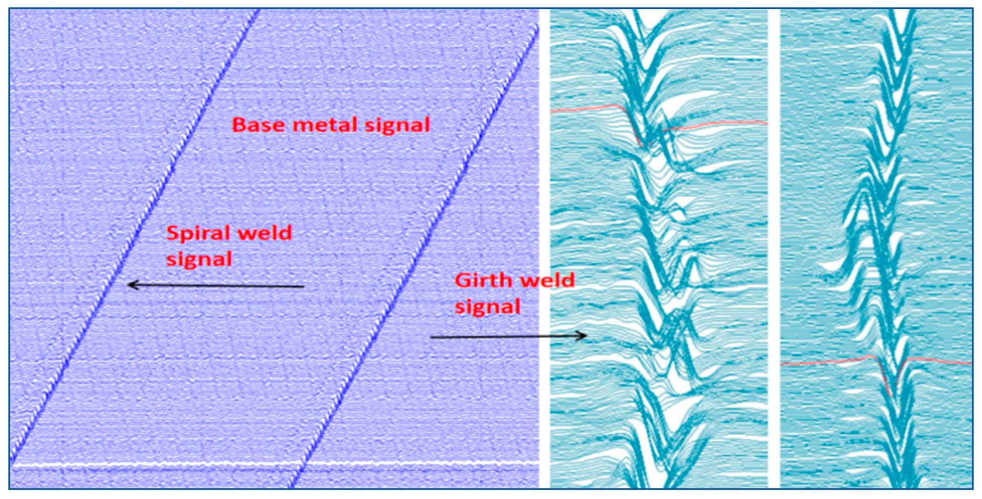
2.1. MFL In-Line Inspection

MFL in-line inspection technology refers to the use of strong magnets mounted on the MFL in-line inspection tool to conduct saturation magnetization on the pipe wall, and magnetic flux leakage occurs due to the low permeability at the defect sites in the presence of defects, such as metal loss. The MFL in-line inspection tool probe detects changes in the magnetic field, leading to corresponding modifications in the MFL signal image [38,39]. Then, a data analyst interprets the data to determine the pipe wall defects. Figure 1 shows a schematic diagram of the MFL inline inspection technology, Figure 2 illustrates a schematic diagram of the defects detected via the magnetic leakage field, and Figure 3 presents an image of the MFL signal including base metal signal, spiral weld signal and girth weld signal. Since the girth welds of long-distance oil and gas pipelines are mainly produced via manual welding, the MFL in-line inspection signals at these locations are highly irregular. Therefore, it is impossible to determine the presence or type of defect in a girth weld via traditional data analysis.

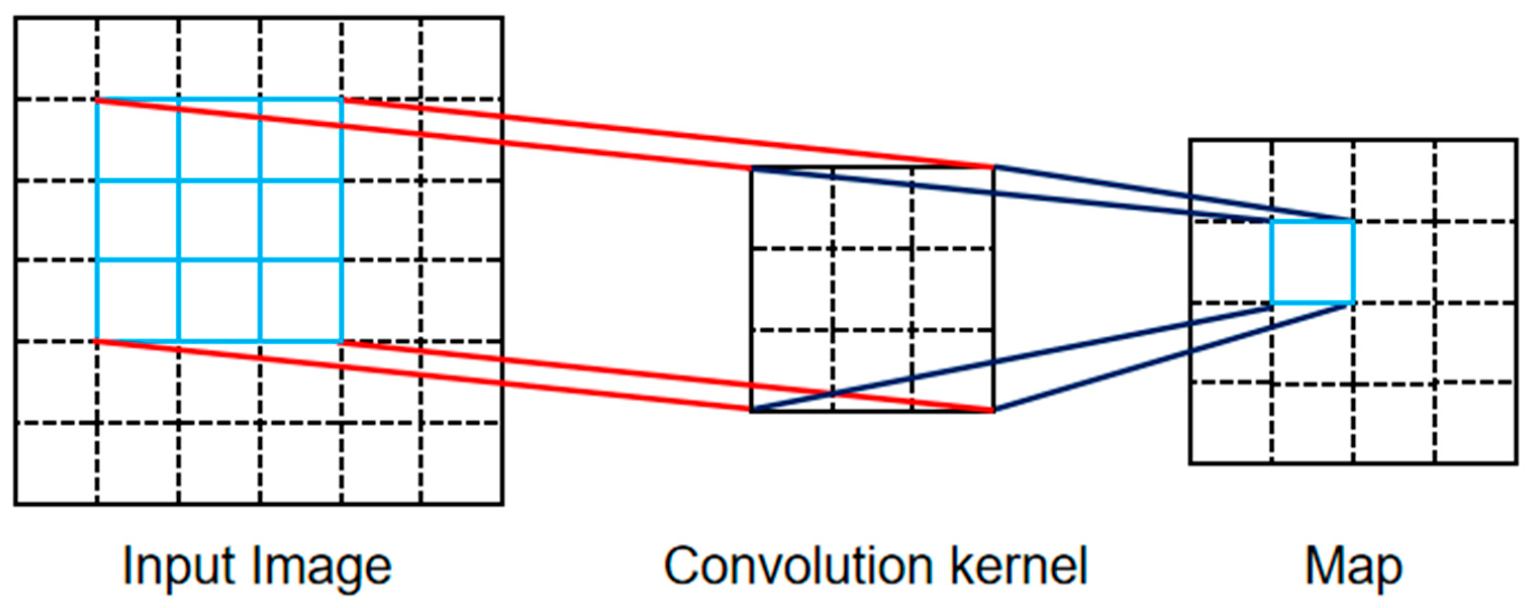
2.2. Convolutional Neural Network (CNN)

In recent years, CNNs have been widely applied in image processing. Image classification using deep CNNs represents an integrated method for image feature extraction and classification recognition [40]. A CNN mainly comprises a convolutional layer, a pooling layer, and a full connection layer. The convolutional layer consists of multiple convolutional units, while different input layer features are extracted via operation. Figure 4 shows a schematic diagram of the convolutional process. The pooling layer can further filter the image features, determine important feature information, reduce the number of parameters, simplify the calculation procedure, and improve the training speed. The full connection layer analyzes the data extracted from the convolutional and pooling layers and classifies them. Feature extraction models can extract higher-dimensional features and prevent the limitation presented by manual feature recognition. All these models are capable of excellent classification in international open data sets. This paper mainly uses ResNet-50 to classify the MFL in-line inspection images of girth welds. Effective CNN development can be attributed to a large number of samples in the data set, while the classification capability of the model is poor when the sample size of the data set is small. The deep convolutional generative adversarial network (DCGAN) proposed in recent years is capable of image generation, which can effectively increase the number of samples in the data set. This paper uses the improved DCGAN model for data set enhancement.

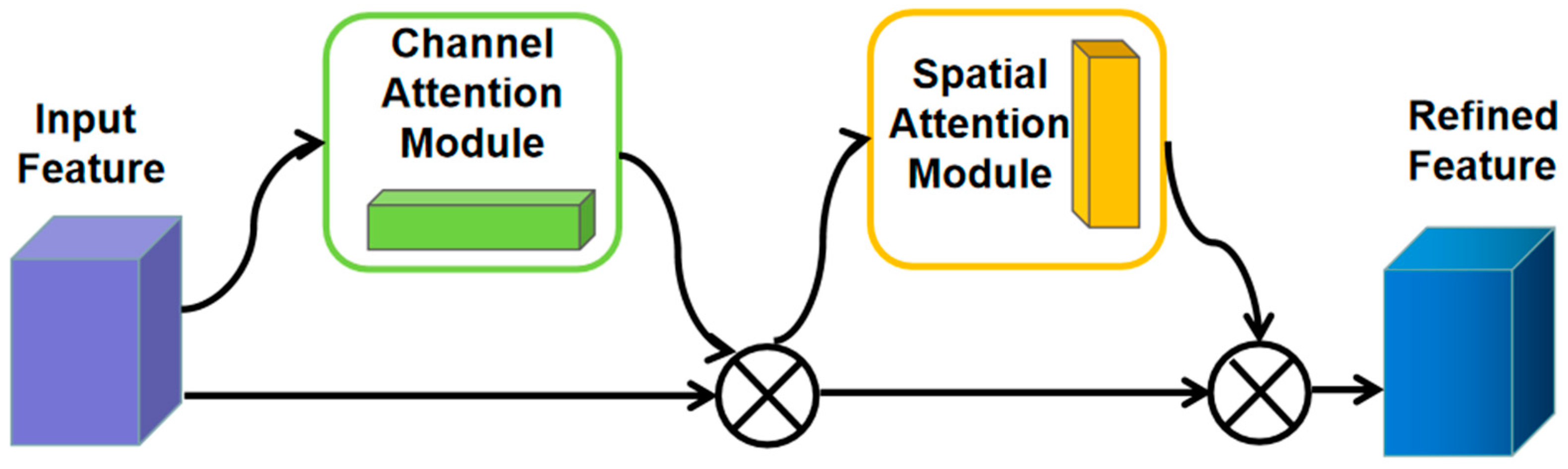
2.3. The Attention Mechanism

This refers to the human visual attention mechanism in the internal structure of the neural network. By assigning weights, the neural network can focus on important information, restrict unimportant information, reduce noise data, decrease the targeted learning of key features by the neural network, reduce computation, enhance feature expression ability, and improve the signal-to-noise ratio, consequently improving the generalization ability of the model [41]. The Convolutional Block Attention Module (CBAM) is a classic mixed attention module that integrates spatial and channel attention. It is simple and efficient, benefits from the universality and lightness of CBAM, and does not consider the computational cost of the module. It can be integrated into the CNN of any structure or with a traditional CNN for training and is responsible for feature optimization during the forward and backward propagation of CNN. Figure 5 presents a schematic diagram of CBAM. In this paper, the CBAM is embedded into the ResNet-50 network, focusing on effective key features and improving the recognition rate and robustness of the network model.

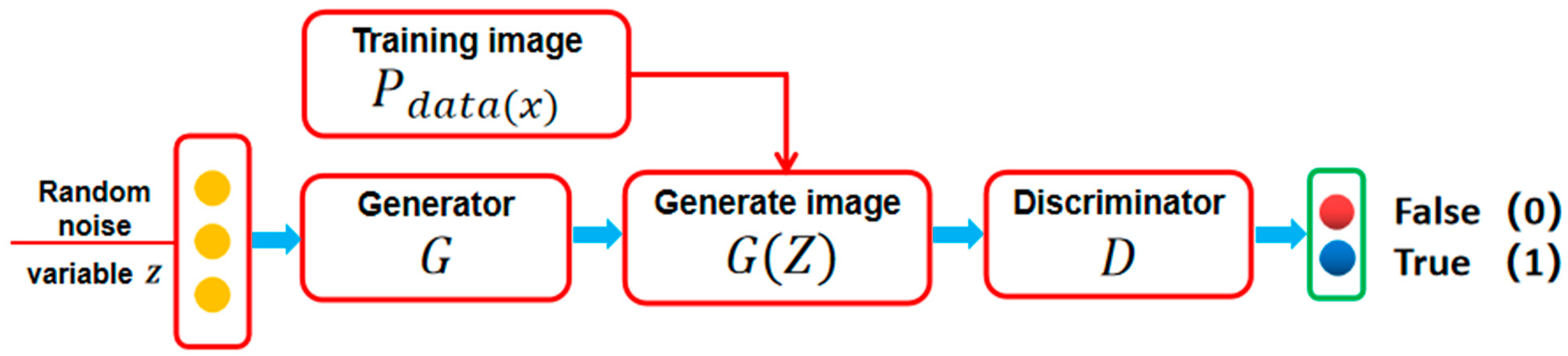
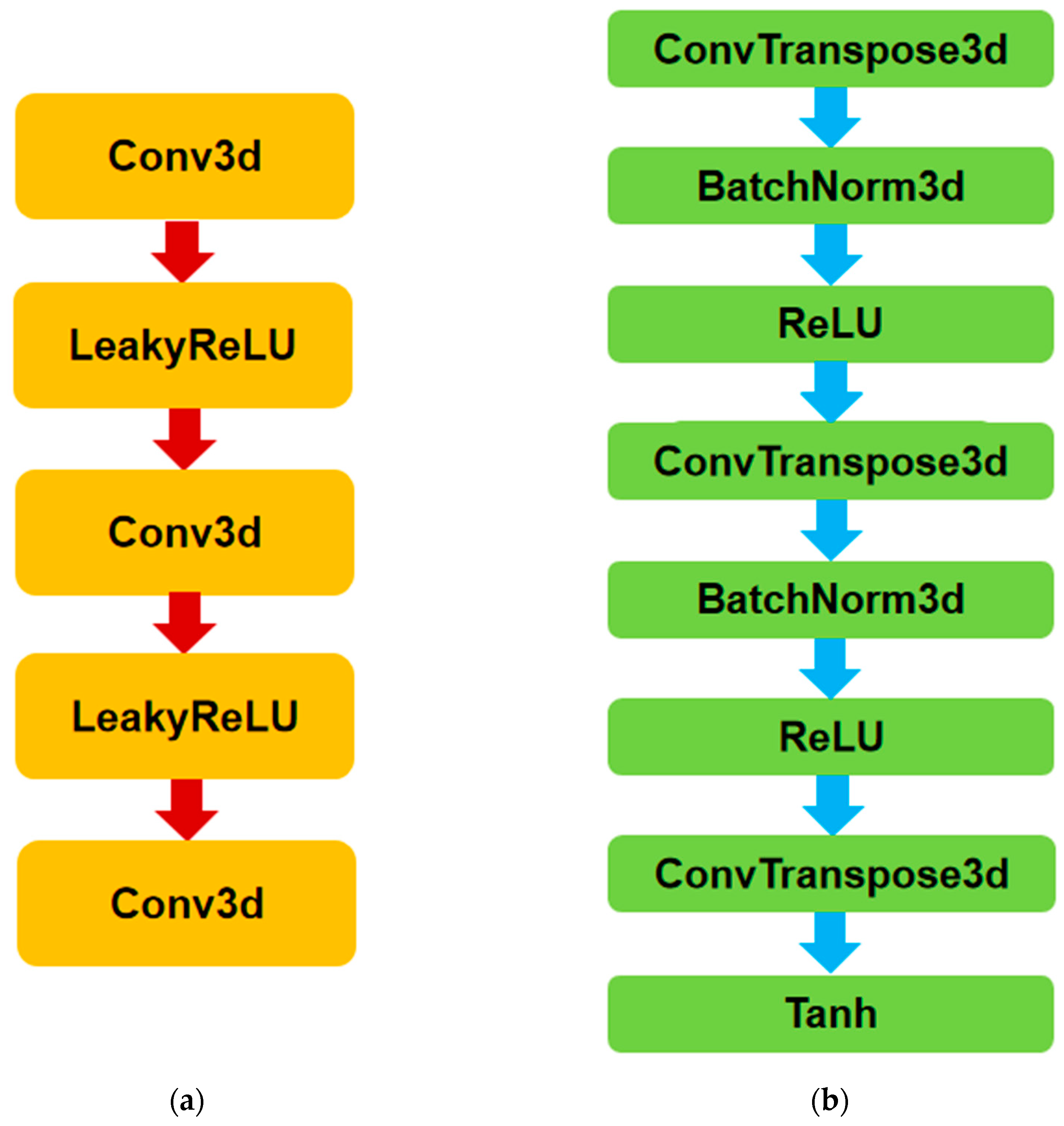
2.4. Deep Convolutional Generative Adversarial Network (DCGAN)

In 2014, Goodfellow et al. [42] from the University of Montreal proposed the Generative Adversarial Network (GAN), representing a network model with an excellent generative effect. The GAN is mainly composed of generators and discriminators, the specific execution process of which is shown in Figure 6.
First, an input noise 𝒵 is set, which conforms to a random distribution, after which the generator generates new data. The calculation formula of Generator G is shown in Equation (1):
minV ( D , G ) G = E 𝒵 ~ P 𝒵 ( 𝒵 ) [ log ( 1 D ( G ( 𝒵 ) ) ) ]
Here, E is the mathematical expectation, P Z ( Z ) is the Gaussian noise distribution, and D ( G ( Z ) ) is the output probability of the discriminator for the forged input sample. The goal of the training is to make G as small as possible. The new data generated by the generator and the original data P d a t a ( x ) are sent to discriminator D, which distinguishes the authenticity of the generated data. The calculation formula of discriminator D is shown in Equation (2):
maxV ( D , G ) D E X ~ P d a t a ( x ) [ log ( D ( X ) ) ] + E Z ~ p Z ( Z ) [ log ( 1 D ( G ( Z ) ) ) ]
Here, D ( X ) is the output probability of the discriminator for the real input sample. The larger the value of discriminator D, the more realistic the generated data. GAN is trained to make the generated data “fool” the discriminator as much as possible. If the discriminator cannot distinguish the original from the generated data, the generated data is confirmed as authentic. At the same time, the discriminator adjusts its discriminant ability to form an adverbial game relationship with the generator. Its theoretical formula is shown in Equation (3):
min   G max D V ( D , G ) = E X ~ P data ( x ) [ log ( D ( X ) ) ] + E z ~ P z ( z ) [ log ( 1 D ( G ( Z ) ) ) ]
Equation (3) shows that V ( D , G ) must be maximized for the discriminator, requiring the maximization of D ( X ) and minimization of ( G ( Z ) ) . For a generator, V ( D , G ) must be minimized and is consequently only related to the second term on the right, which is the maximization of D ( G ( Z ) ) .
Although GAN can expand the data set, it presents some challenges, such as vanishing gradient and collapse mode. In 2016, Radford et al. [43] proposed a deep convolutional generative adversarial network (DCGAN). Instead of a multi-layer perceptron MLP, a CNN replaces it, rendering the overall network model differentiable and improving the quality of data generation. The main structures of the DCGAN discriminator and generator are shown in Figure 7.
Since DCGAN continues to use the loss function of GAN, it is necessary to carefully balance the optimization of generator and discriminator during the training process to avoid training instability and even gradient explosion. This paper proposes an improved DCGAN_GP method with gradient punishment based on DCGAN. This method adopts the generator and discriminator structure of DCGAN and adds an additional gradient penalty to the discriminator loss function. Firstly, samples   x r and x g are obtained from the real sample space p r and generated sample p g , respectively, after which the value is randomly inserted between the real sample p r and generated sample p g , as shown in Equations (4):
x r ~ p r ,   x g ~ p g ,   ε ~ U [ 0 , 1 ] ,   x t = ε x r + ( 1 ε ) x g
where   U   [ 0 , 1 ] means that the distribution probability of the same interval on [ 0 , 1 ] is equally possible. The original loss function of the discriminator is shown in Equation (5):
L o r i g i n a l = E x ~ P g [ D ( x ) ] E x ~ P r [ D ( x ) ]
where E x ~ P g [ D ( x ) ] represents the mathematical expectation of the sample generation as the input of the discriminator. E x ~ P r [ D ( x ) ] represents the mathematical expectation when the input of the discriminator is a real sample. The gradient penalty term is shown in Equation (6):
G P = E x ~ x t [ ( x D ( x ) 2   1 ) 2 ]
where x D ( x ) represents the gradient in the x direction of the output value of the discriminator and E x ~ x t represents the mathematical expectation when the discriminator input denotes random interpolation sampling x t . The discriminator loss function of DCGAN-GP is shown in Equation (7):
L ( D ) = L o r i g i n a l + GP
GP introduced in the original DCGAN, solves the problems of gradient disappearance and gradient explosion in the original DCGAN. The improved DCGAN_GP network model for data set enhancement addresses the challenge of few data samples in the original data set.

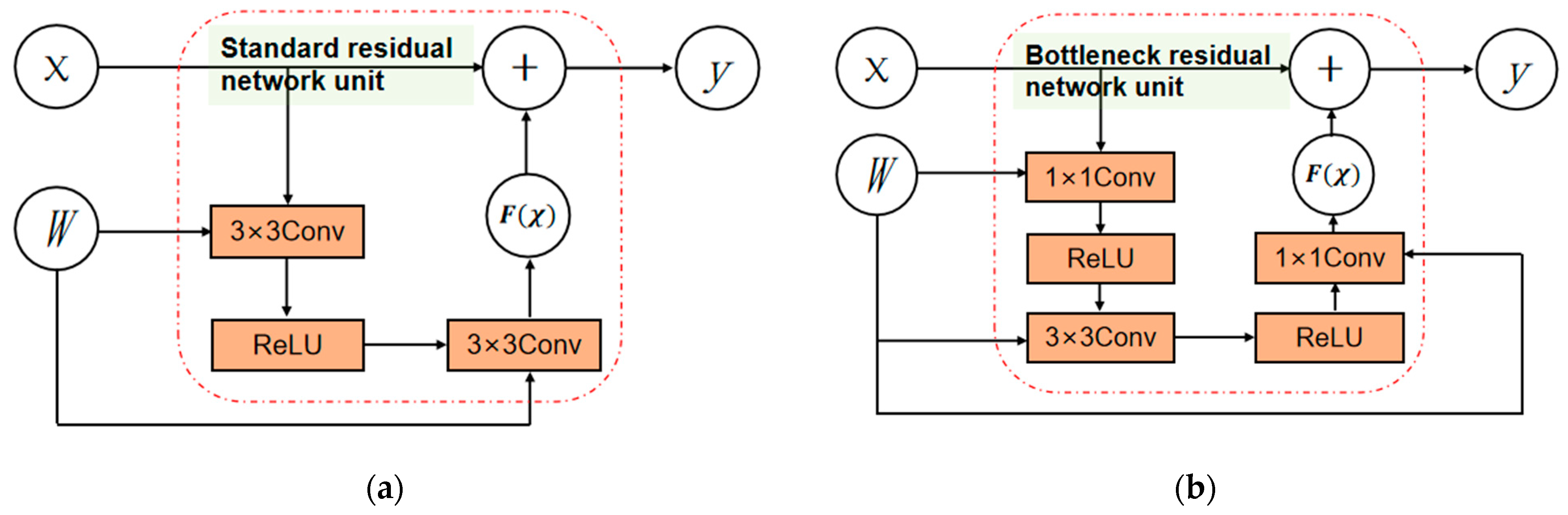
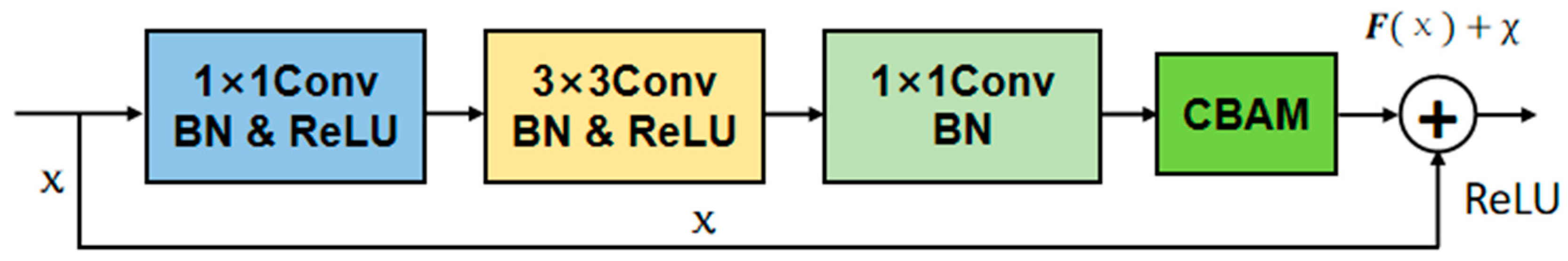
2.5. Residual Network (ResNet)
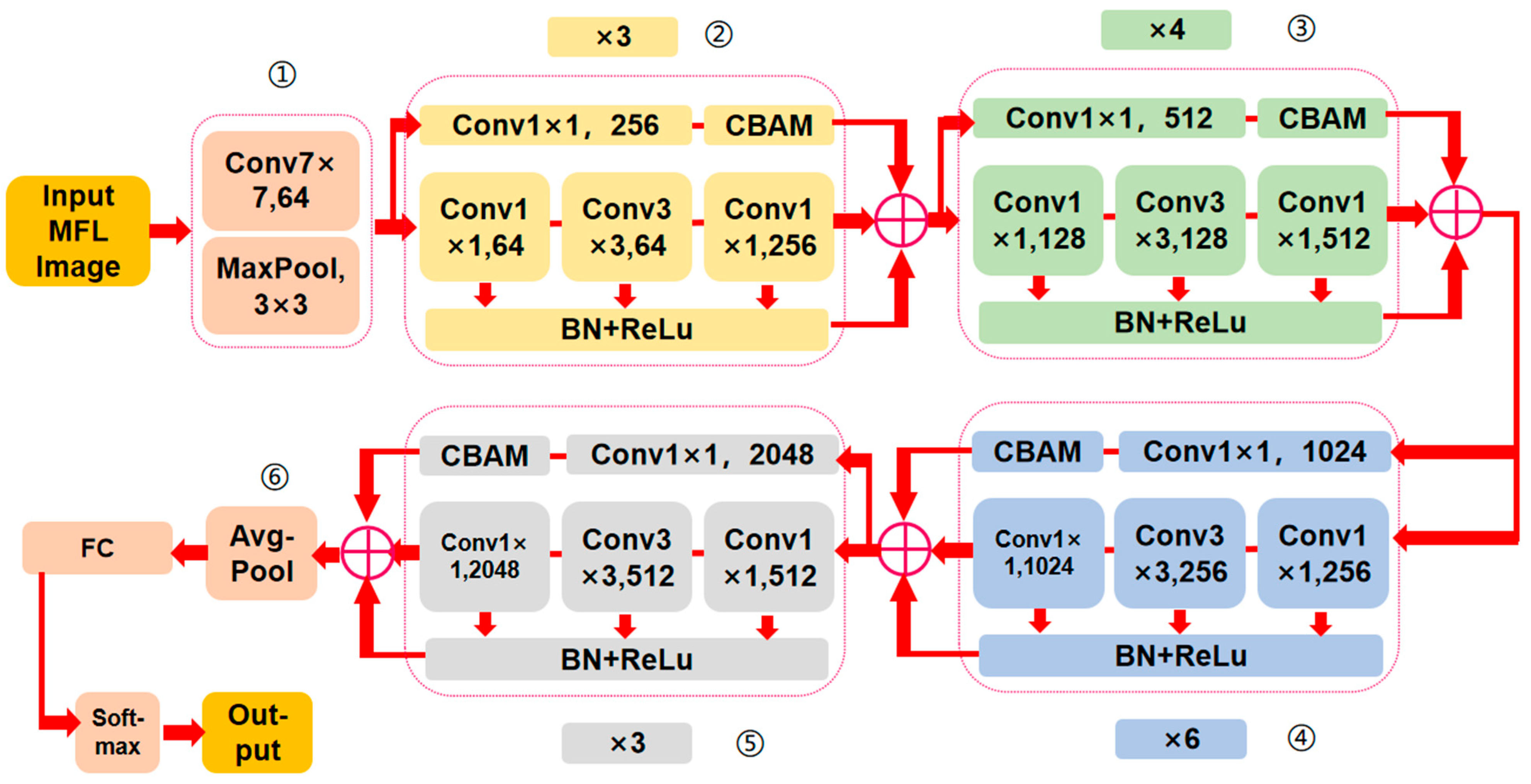
In 2016, Kaiming He et al. [27] proposed the ResNet model at the computer vision and pattern recognition (CVPR) conference to address the degradation caused by gradient dispersion and other challenges presented by deep-seated networks during training via identity mapping and enhancing the learning ability and computing performance of the complex feature extraction mode. The core idea of residual learning is to fit the neural network to the identity mapping x = H ( x ) and introduce the short-circuit mechanism and identity mapping into its network model to design the residual unit, as shown in Figure 8, where (a) is the standard residual unit, and (b) is the bottleneck residual unit.
Here, x n represents the input of the residual unit at the nth layer, while its final output y n is shown in Equation (8); W n is the input of the residual unit at the nth layer, and the objective function F is the residual function that the neural network needs to learn. Due to identity mapping, the residual function F is the residual y n x n between the output and the input.
y n = F ( x n , W n ) + x n
The ResNet neural network model has different implementation models according to the number of convolutional layers in its internal structure. Shallow neural networks, such as ResNet-18 and ResNet-34, use standard residual units for the feature layer, while deep neural networks, such as ResNet-50, ResNet-101, and ResNet-152, use bottleneck residual units. Each ResNet model is shown in Table 1. According to Table 1, the ResNet-50 model displays both a feature learning ability and computing performance. This paper uses this neural network model to classify the MFL in-line inspection images of girth.
Since the data set contains a substantial amount of invalid information, a CBAM is added to ResNet-50, allowing the improved deep learning network model to pay more attention to the effective key features while reducing or ignoring some invalid feature information and improving its recognition rate and robustness. According to Section 2.3, CBAM is a lightweight attention model that can be embedded into the bottleneck residual unit, as shown in Figure 9. The improved ResNet-50 with an embedded CBAM is shown in Figure 10, showing the network parameters.
There are 174 layers in total in the improved ResNet-50 network. As shown in Figure 10, the improved network mainly includes the Convolutional layer, MaxPool layer, Residual unit embedded with CBAM, AvgPool layer, etc. (marked with serial number). The size of the input picture is 64 × 64, after the AvgPool layer, becoming 1 × 1. Detailed parameters for network structure and MFL image are shown in Table 2.
Image classification using the deep learning method requires balanced distribution among various types of data sets. Therefore, it avoids the deep learning network model, focusing on a large number of samples or samples with more easily identifiable features, which may affect the overall identification accuracy of the model and cause poor performance. Loss functions are usually introduced into network models to solve the problem of unbalanced data sets.
In this paper, the Focal Loss function proposed by Lin et al. [44] is introduced into the improved ResNet50_CBAM network model. This function designs the weight according to the prediction probability of samples, in which samples with a higher probability of prediction are regarded as easily identifiable samples and given a lower weight, while those with a low probability of prediction are regarded as samples difficult to learn and given higher weights. Compared with the commonly used cross entropy (CE) loss function, the Focal Loss function can dynamically adjust the weight during network model training, which is more flexible. With dichotomies as an example, the relevant comparison is shown in Equations (9)–(11):
The CE loss function of a single sample ( x , y ) is:
C E ( x , y ) = ( y log p + ( 1 y ) log ( 1 p ) )
where y { 0 , 1 } is the category label, and p [ 0 , 1 ] is the prediction probability of the sample belonging to category 1.
Regarding the classification problem of unbalanced data sets, the model can improve the classification of minority samples by adjusting the weight of majority and minority samples, which can be expressed as follows:
α _ b a l a n c e d _ C E ( x , y ) = ( α y l o g p + ( 1 y ) l o g ( 1 p ) )
The Focal Loss function is expressed as:
F L ( x , y ) = ( y ( 1 p ) γ l o g p + ( 1 y ) p γ l o g ( 1 p ) )
where γ is the adjusting coefficient.
Therefore, compared with the CE loss function, the Focal Loss function is more flexible for weight adjustment. This paper uses the improved ResNet-50_CBAM deep learning network model with Focal Loss for data set classification.
ResNet-50_CBAM, an improved ResNet-50 network model, whose robustness is improved by using CBAM to pay more attention to the effective feature and ignoring some invalid features of the data set, is used to classify the data set after enhancement. At the same time, the Focal Loss function, introduced into the ResNet-50_CBAM, helps the model dynamically adjust the weight during training and avoids the model from focusing on a large number of samples or samples with more easily identifiable features. Thus, the improved ResNet-50_CBAM network model performs better than the original model.

3. Methods

This paper used a CNN to classify data sets, a process that was mainly divided into the following three steps: (1) The original data set was established. (2) The improved deep convolutional generative adversarial network DCGAN_GP_CBAM was used to enhance the data sets. (3) The enhanced data set was used to iteratively train the improved residual network ResNet-50_CBAM.

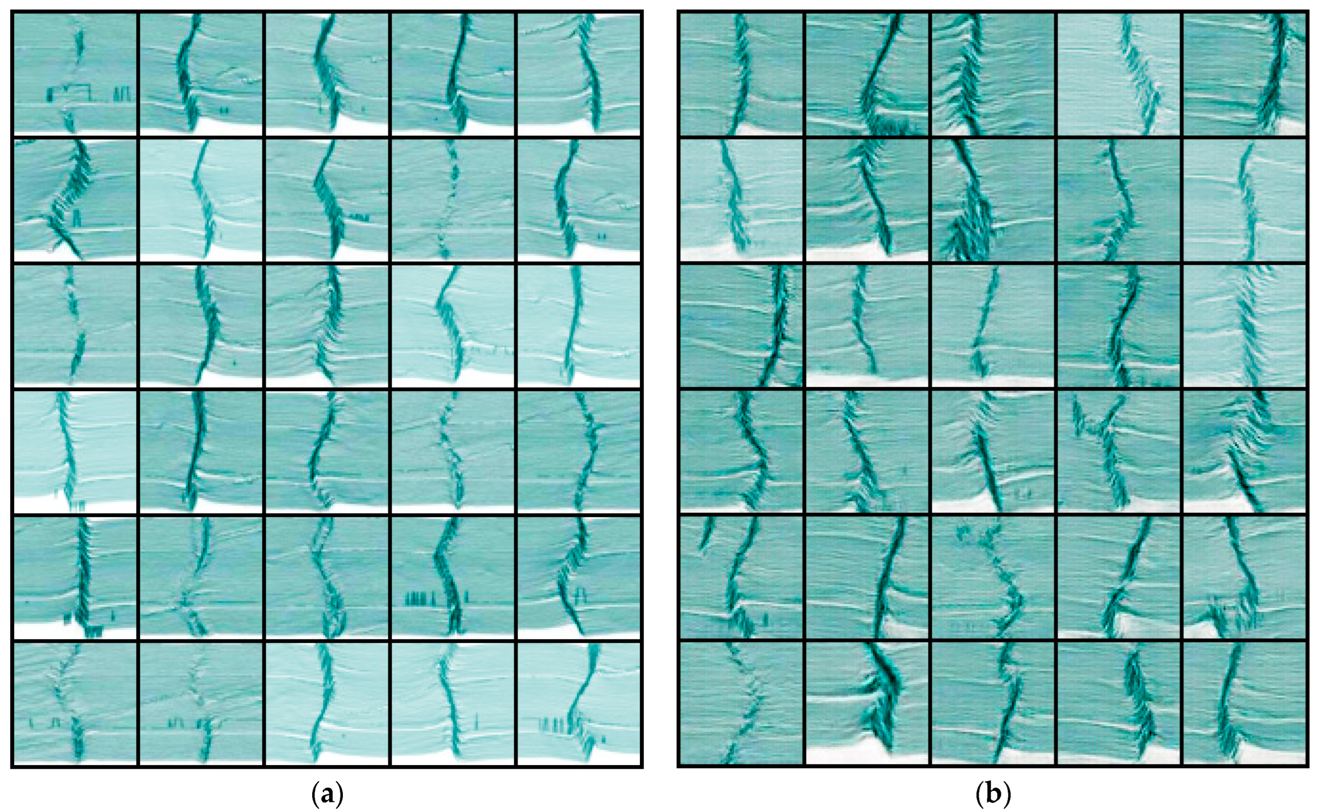
3.1. Establishment of the Original Data Set

The radiographic testing results of 1462 girth welds excavated from a long-distance natural gas pipeline were collected and aligned with the girth welds recognized via MFL in-line inspection. Screenshots were taken of the MFL in-line inspection signals of the girth welds and labeled with radiographic testing results, such as circular defect, strip defect, incomplete fusion, incomplete penetration, crack, pit, and undercut. The number of labels in the data set is shown in Table 3.
The sum of incomplete fusion, incomplete penetration, crack, pit, and undercut was 60, with a 4.1% ratio. For such a small proportion, this paper only selected samples containing two kinds of labels, which are circular defects and strip defects, to establish the original sample set, using a total of 1402 samples; 60 circular defects and 36 strip defects were selected as the testing set from this original data, and the remainders were enhanced.

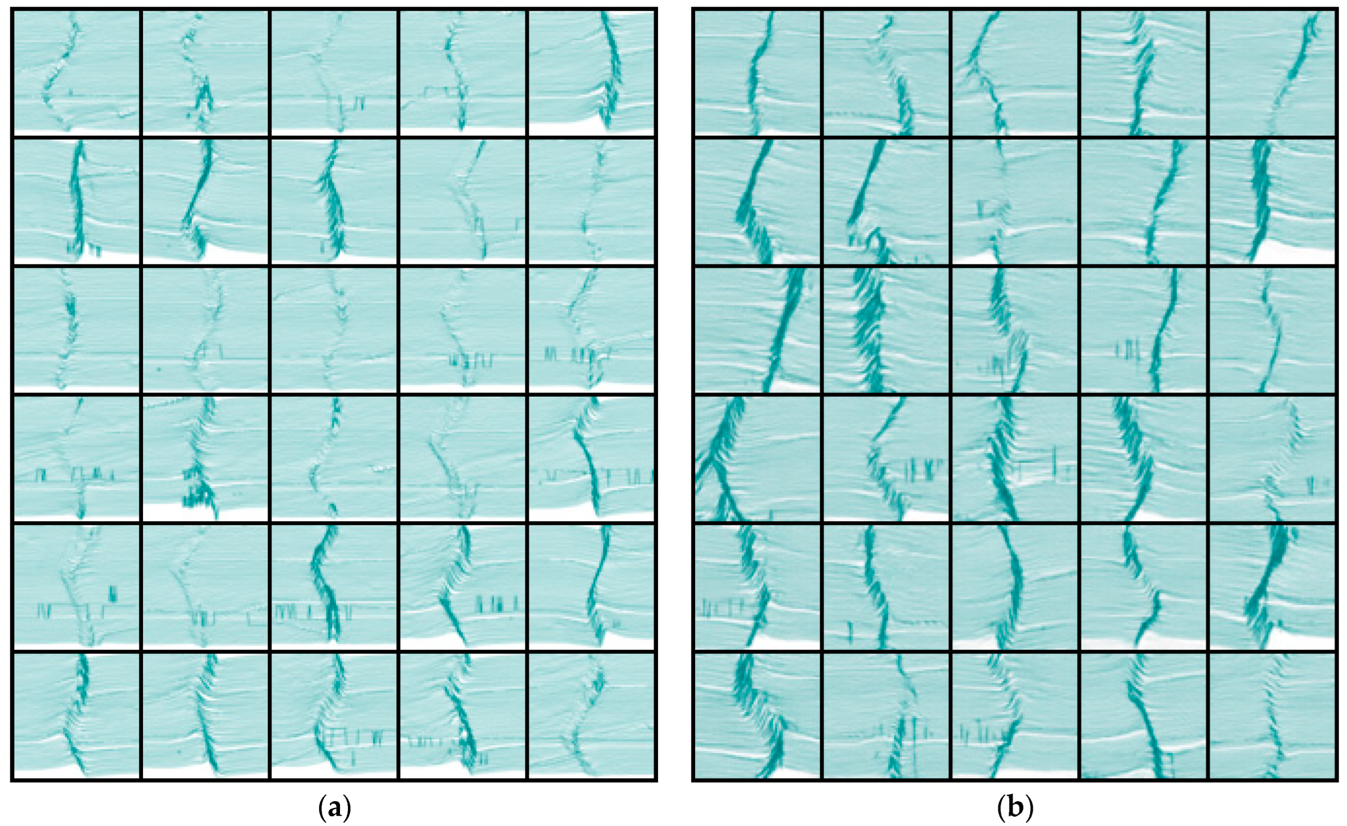
3.2. Data Set Enhancement

As described in Section 2.4, a DCGAN was used to enhance the original data set (without testing set). This paper used Pytorch to build the deep learning framework and Python version 3.6.4 as the programming language. The hardware platform included an Intel ® Core (TM) i7-10750H with 16 GB CPU memory and NVIDIA GeForce RTX 3060 Laptop with 6 GB GPU memory. The data set (without testing set) was expanded to a total of 2670 samples, including 1660 circular defects and 1010 strip defects. Compared with the original data set (without testing set), the number of samples in the enhanced data set increased, as shown in Table 4. Figure 11 and Figure 12 show the “pseudo circular defects data set” and “pseudo strip defects data set” after data enhancement, indicating that the newly generated data had a good effect.

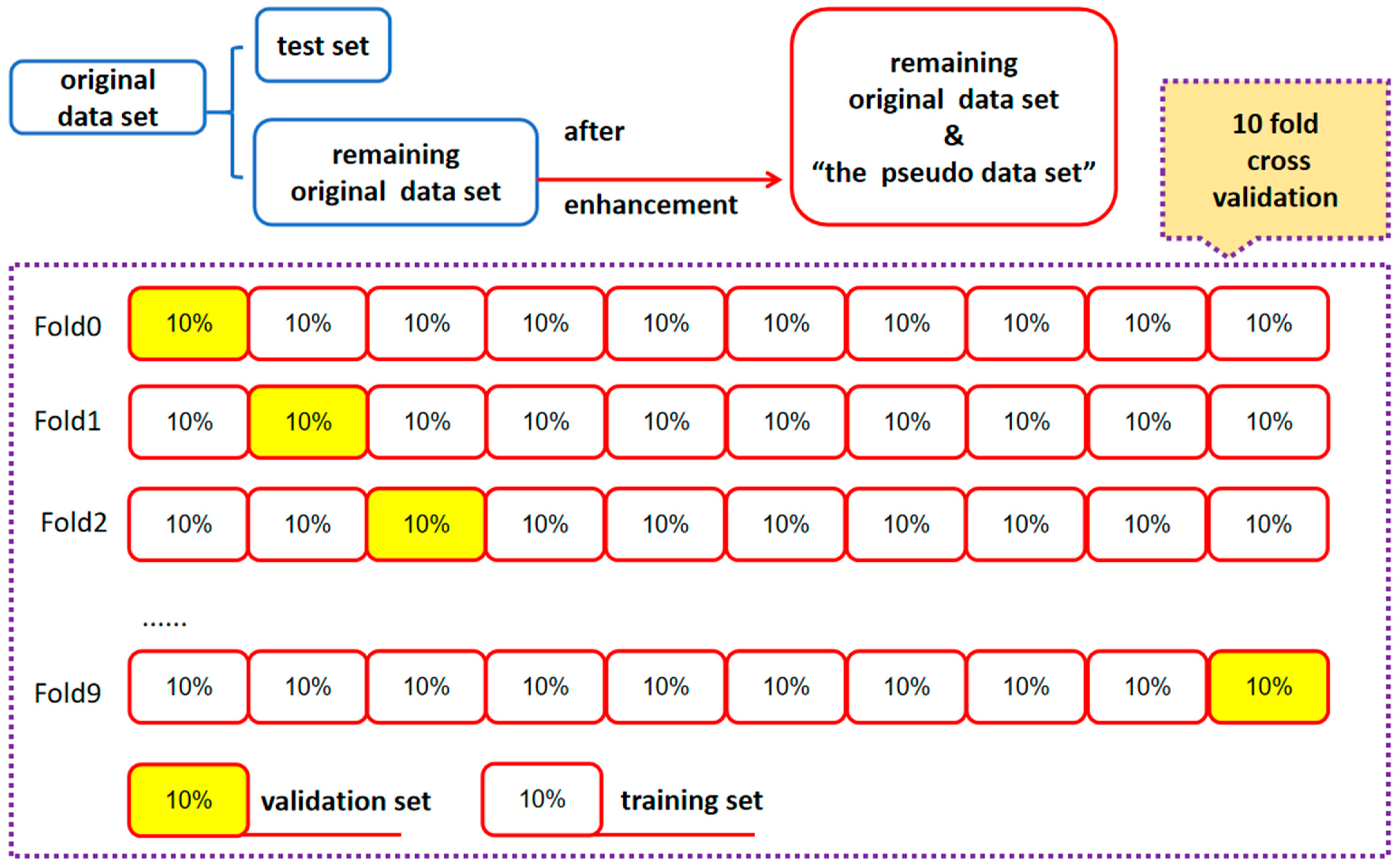
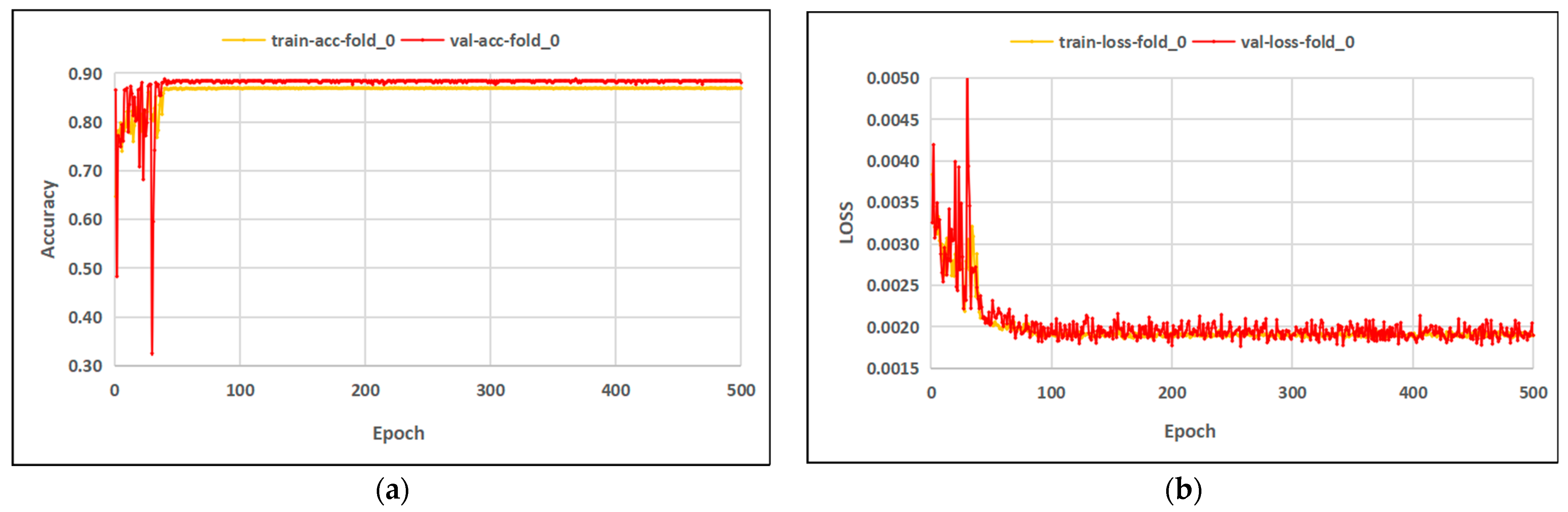
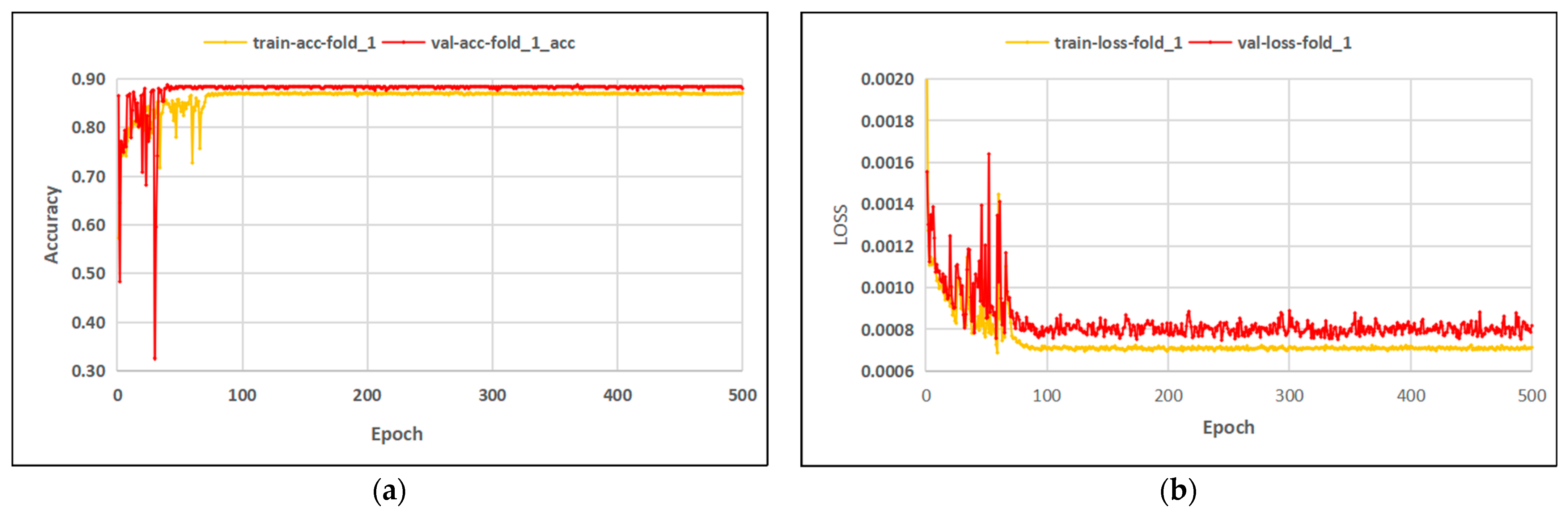
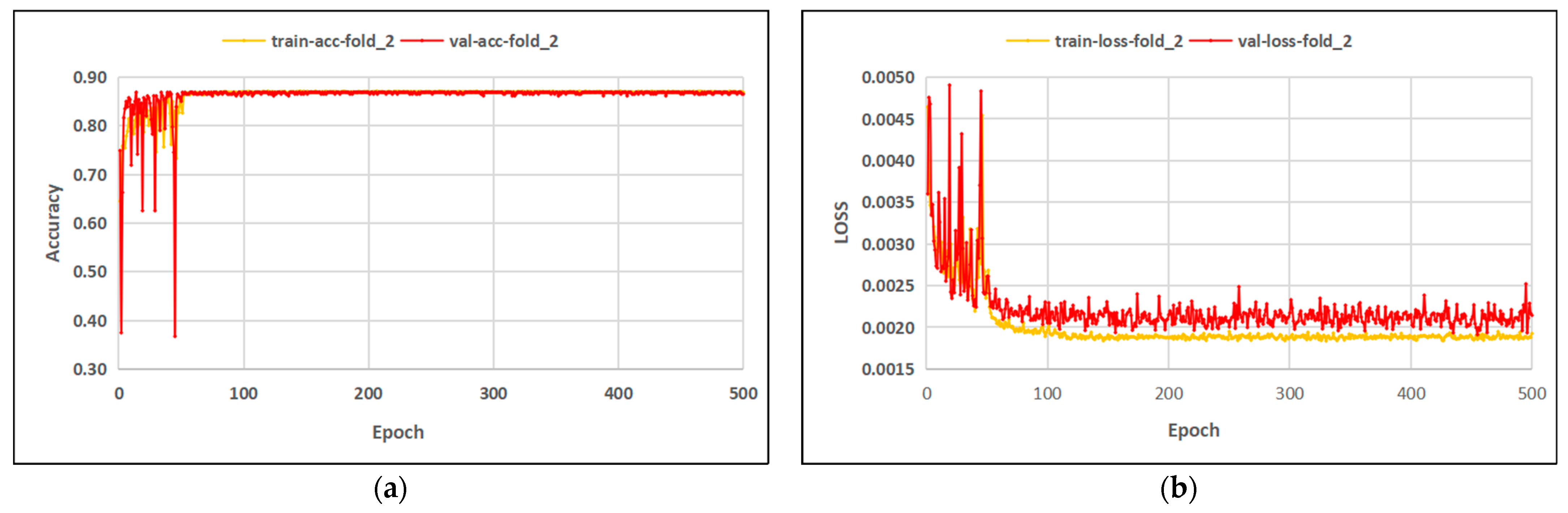
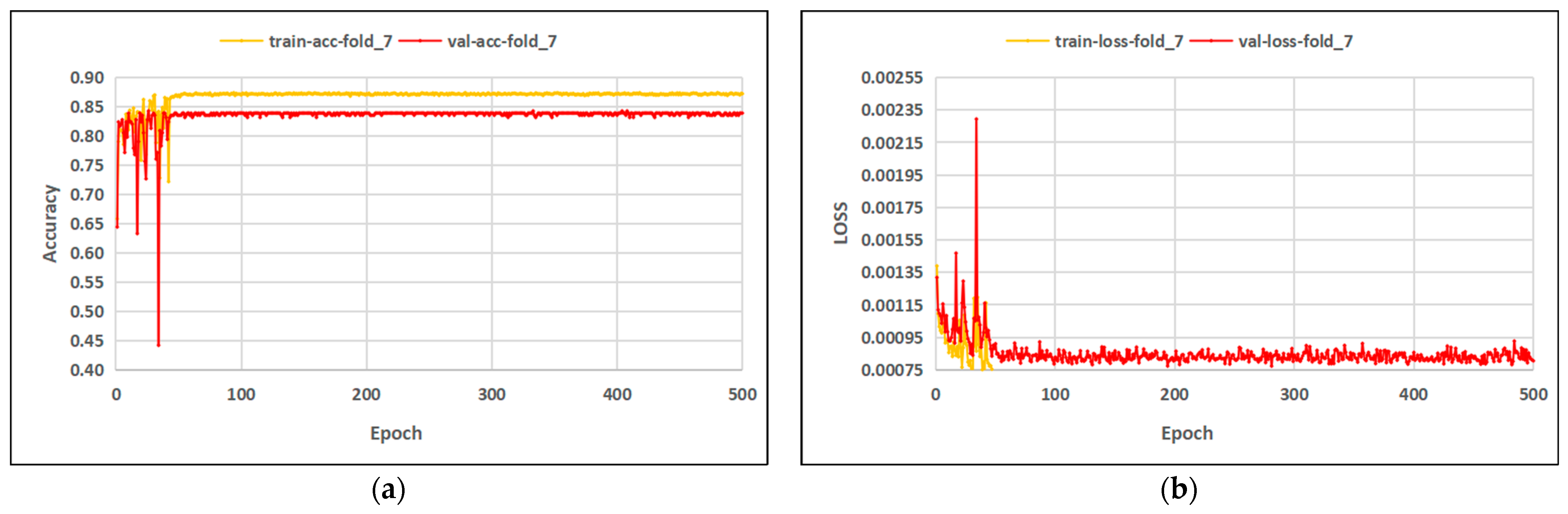
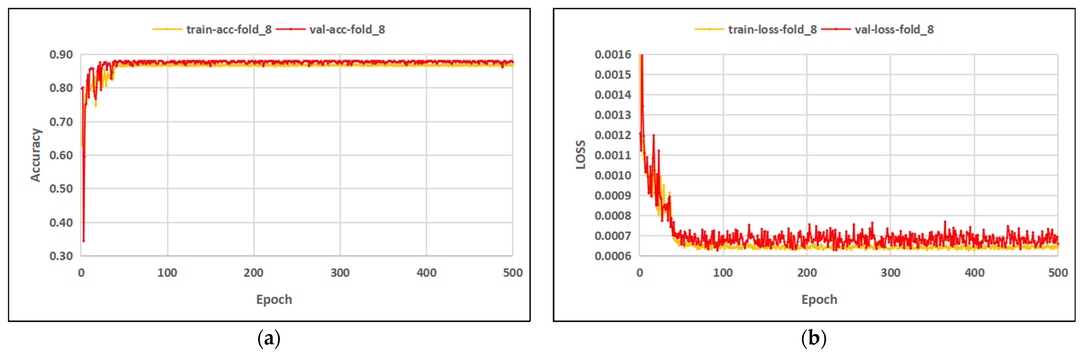
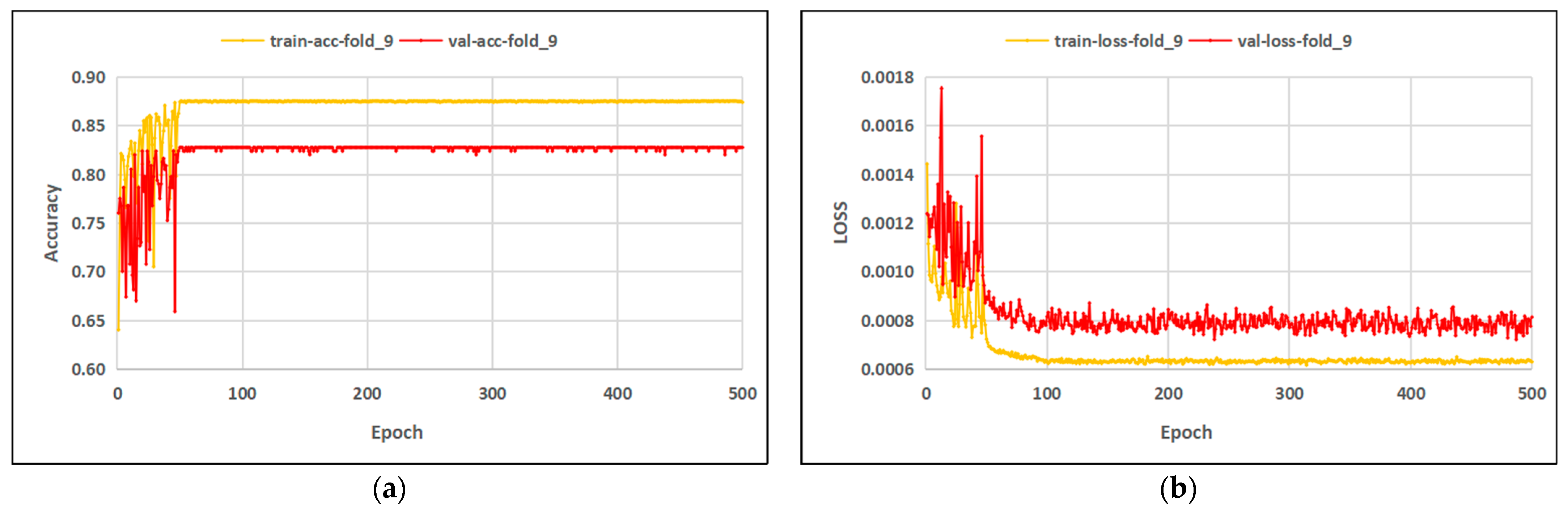
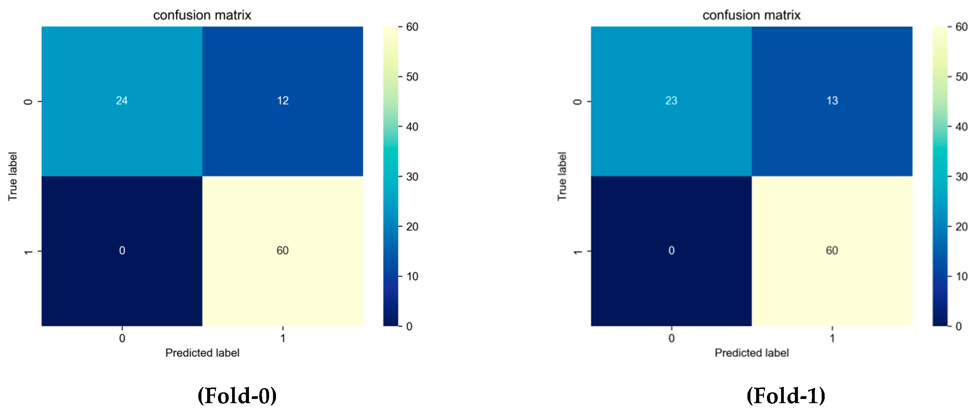
3.3. Data Set Classification

As described in Section 2.5, this paper selected the improved ResNet-50_CBAM network as the classifier. Pytorch was employed for the deep learning framework, while Python version 3.6.4 was used as the programming language. The hardware platform was an Intel (R) Core (TM) i7-10750H with 16 GB CPU memory and NVIDIA GeForce RTX 3060 Laptop with 6 GB GPU memory.
For the remaining data set (without testing set) after enhancement, it was divided into a training set and a validation set in the ratio of 9:1; the data selection process is shown in Figure 13, and cross-validation was carried out 10 times. In every fold, the network was trained and validated for 500 iterations. The accuracy and loss curve for 10-fold-cross validation is shown in Figure 14, Figure 15, Figure 16, Figure 17, Figure 18, Figure 19, Figure 20, Figure 21, Figure 22 and Figure 23. The results showed that the loss of the improved ResNet-50_CBAM network model tends toward 0, and the accuracy rate is greater than 80%. After calculation, the average accuracy is 87.2% and the average loss rate is 0.013. All these results indicate that the improved model displayed strong generalization ability and robustness and has a good classification effect.
Then, the training result was tested in the testing set. In this paper, multiple indicators were used as the evaluation basis for the classification effect. The accuracy rate, the recall rate, and the F1-score are shown in Table 5; the confusion matrix is shown in Figure 24.
All the results above show that the improved ResNet-50_CBAM network has a good classification effect. The improved model confuses strip defects to a high degree, with an accuracy of 67%, indicating that the recognition method of strip defects by this model needs to be improved. The model has a low level of confusion with circular defects, with an accuracy of nearly 100%, indicating that the improved model has a very strong ability to identify circular defects.
Therefore, the improved ResNet-50_CBAM network model is capable of accurately classifying the MFL images of the pipeline girth welds.

4. Conclusions and Discussion

(1)
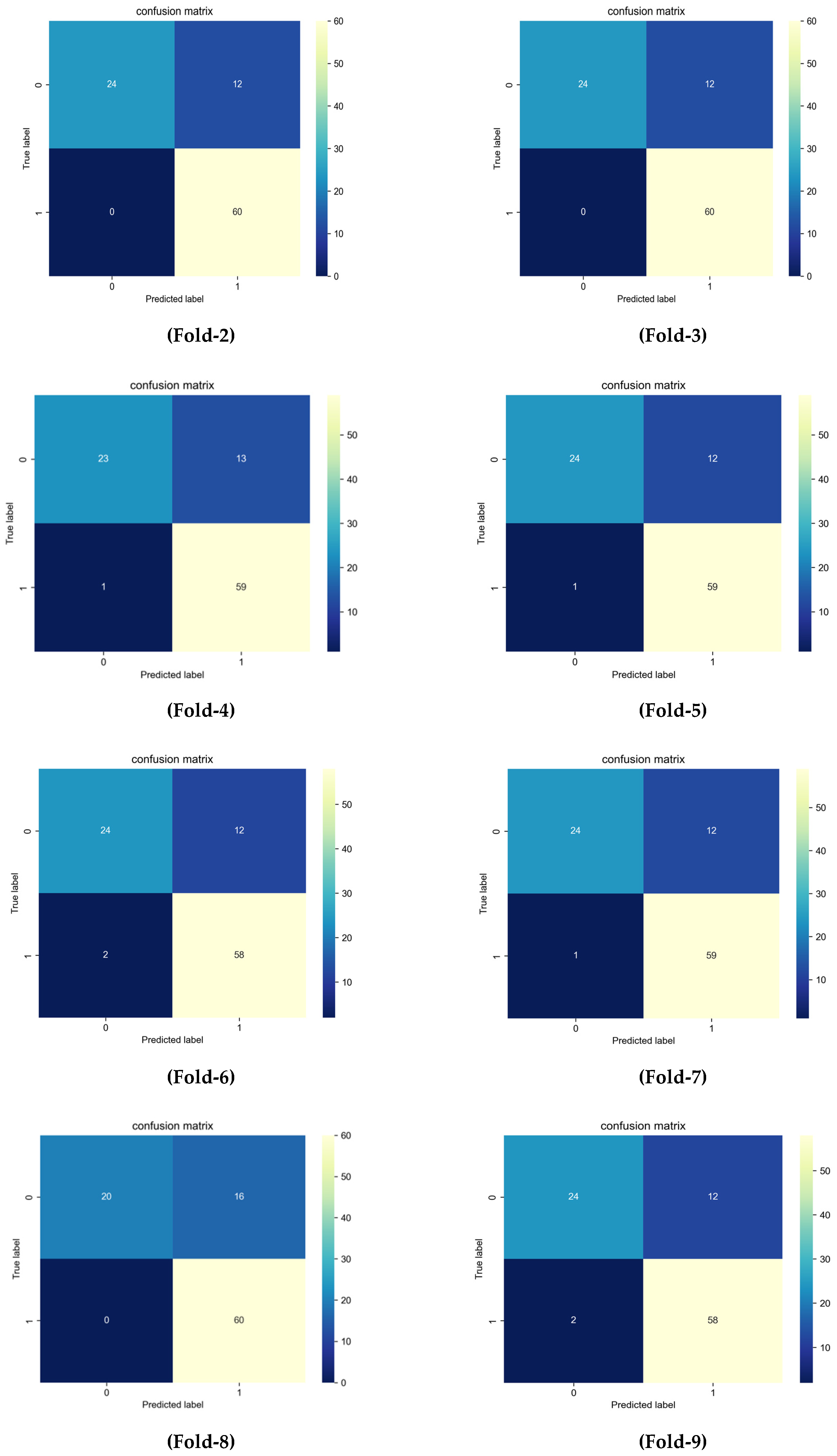
The DCGAN_GP can enhance the data set of girth weld signal images obtained via MFL in-line inspection. The improved ResNet-50_CBAM displays a strong generalization ability and robustness and can effectively classify with the data set of girth weld signal images obtained via MFL in-line inspection with an accuracy rate of over 80%. However, the improved model confuses strip defects to a high degree with an accuracy of 67%, so the recognition method of strip defects by this model needs to be improved in the following study.
(2)
The incomplete fusion, incomplete penetration, cracks, pits, and undercuts pose greater threats to the safety of girth welds. However, these types were not selected as test objects for this study because they represent an insufficient proportion of the data set. Future efforts should focus more on challenging expanding the data set and realizing multi-classification for the data set.
(3)
In the next study, the GoogleNet model, VGG model, and other models should be improved to classify the database. The classification results should be compared to those of this paper to select a better classification method.
(4)
This pipeline section will soon complete the second round of MFL in-line inspection. The new data set should be classified using the improved model. Pipeline operators can make comprehensive judgments based on both classification results, thereby assisting pipeline operators in strengthening the safety management of girth welds.
(5)
It is also possible to use other nondestructive testing results, such as ultrasonic and TOFD as labels for girth weld MFL signal images to establish new data sets. The classification results are of significance to pipeline safety management.

Author Contributions

Conceptualization, L.G. and S.D.; methodology, L.G., S.D. and W.Q.; software, L.G. and W.Q.; validation, L.G. and W.Q.; formal analysis, L.G. and S.D.; investigation, L.G. and S.D.; resources, L.G. and D.P.; data curation, L.G. and S.D.; writing—original draft preparation, L.G. and W.Q.; writing—review and editing, L.G., S.D., W.Q. and D.P.; visualization, L.G. and W.Q.; supervision, L.G. and S.D.; project administration, L.G. and S.D.; funding acquisition, L.G. and S.D. All authors have read and agreed to the published version of the manuscript.

Funding

This research received no external funding.

Informed Consent Statement

Not applicable.

Data Availability Statement

Not applicable.

Acknowledgments

The author gratefully acknowledge the institutional support provided by PipeChina company.

Conflicts of Interest

The authors declare no conflict of interest.

References

  1. Wang, K.; Xie, K.; Zhang, H.; Qiang, Y.; Du, Y.; Xiong, Y.; Zou, Z.; Zhang, M.; Zhong, L.; Akkurt, N.; et al. Numerical evaluation of the coupled/uncoupled effectiveness of a fluid-solid-thermal multi-field model for a long-distance energy transmission pipeline. Energy 2022, 251, 123964. [Google Scholar] [CrossRef]
  2. Tong, S.-J.; Wu, Z.-Z.; Wang, R.-J.; Wu, H. Fire Risk Study of Long-distance Oil and Gas Pipeline Based on QRA. Procedia Eng. 2016, 135, 369–375. [Google Scholar] [CrossRef]
  3. He, G.; He, T.; Liao, K.; Deng, S.; Chen, D. Experimental and numerical analysis of non-contact magnetic detecting signal of girth welds on steel pipelines. ISA Trans. 2022, 125, 681–698. [Google Scholar] [CrossRef]
  4. Lu, K.-Q.; Lin, J.-Q.; Chen, Z.-F.; Wang, W.; Yang, H. Safety assessment of incomplete penetration defects at the root of girth welds in pipelines. Ocean Eng. 2021, 230, 109003. [Google Scholar] [CrossRef]
  5. Shehab, L.H.; Fahmy, O.M.; Gasser, S.M.; El-Mahallawy, M.S. An efficient brain tumor image segmentation based on deep residual networks (ResNets). J. King Saud Univ. Eng. Sci. 2021, 33, 404–412. [Google Scholar] [CrossRef]
  6. Zhang, X.; Li, Y.; Tao, Y.; Wang, Y.; Xu, C.; Lu, Y. A novel method based on infrared spectroscopic inception-resnet networks for the detection of the major fish allergen parvalbumin. Food Chem. 2021, 337, 127986. [Google Scholar] [CrossRef]
  7. Li, W.; Zhu, D.; Wang, Q. A single view leaf reconstruction method based on the fusion of ResNet and differentiable render in plant growth digital twin system. Comput. Electron. Agric. 2022, 193, 106712. [Google Scholar] [CrossRef]
  8. Loey, M.; Manogaran, G.; Taha, M.H.N.; Khalifa, N.E.M. Fighting against COVID-19: A novel deep learning model based on YOLO-v2 with ResNet-50 for medical face mask detection. Sustain. Cities Soc. 2022, 65, 102600. [Google Scholar] [CrossRef]
  9. Charles, V.B.; Surendran, D.; SureshKumar, A. Heart disease data based privacy preservation using enhanced ElGamal and ResNet classifier. Biomed. Signal Process. Control 2021, 71, 103185. [Google Scholar] [CrossRef]
  10. Ma, K.; Zhan, C.A.; Yang, F. Multi-classification of arrhythmias using ResNet with CBAM on CWGAN-GP augmented ECG Gramian Angular Summation Field. J. Biomed. Signal Process. Control 2022, 77, 103684. [Google Scholar] [CrossRef]
  11. Wang, L.; Yuan, X.; Zong, M.; Ma, Y.; Ji, W.; Liu, M.; Wang, R. Multi-cue based four-stream 3D ResNets for video-based action recognition. Inf. Sci. 2021, 575, 654–665. [Google Scholar] [CrossRef]
  12. Ikechukwu, A.V.; Murali, S.; Deepu, R.; Shivamurthy, R. ResNet-50 vs VGG-19 vs training from scratch: A comparative analysis of the segmentation and classification of Pneumonia from chest X-ray images. J. Glob. Transit. Proc. 2021, 2, 375–381. [Google Scholar] [CrossRef]
  13. Dawod, R.G.; Dobre, C. ResNet interpretation methods applied to the classification of foliar diseases in sunflower. J. Agric. Food Res. 2022, 9, 100323. [Google Scholar] [CrossRef]
  14. Lu, Z.; Bai, Y.; Chen, Y.; Su, C.; Lu, S.; Zhan, T.; Hong, X.; Wang, S. The classification of gliomas based on a Pyramid dilated convolution resnet model. Pattern Recognit. Lett. 2020, 133, 173–179. [Google Scholar] [CrossRef]
  15. Shipway, N.; Huthwaite, P.; Lowe, M.; Barden, T. Using ResNets to perform automated defect detection for Fluorescent Penetrant Inspection. NDT E Int. 2021, 119, 102400. [Google Scholar] [CrossRef]
  16. Taigman, Y.; Yang, M.; Ranzato, M.A.; Wolf, L. DeepFace: Closing the gap to human-level performance in face verification. In Proceedings of the IEEE Conference on Computer Vision and Pattern Recognition (CVPR), Columbus, OH, USA, 23–28 June 2014; pp. 1701–1708. [Google Scholar]
  17. Ossama, A.-H.; Abdel-Rahman, M.; Hui, J.; Penn, G. Applying convolutional neural network concepts to hybrid NN-HMM model for speech recognition. In Proceedings of the IEEE International Conference on Acoustics, Speech and Signal Processing (ICASSP), Kyoto, Japan, 25–30 March 2012; pp. 4277–4280. [Google Scholar]
  18. Ossama, A.-H.; Abdel-Rahman, M.; Hui, J.; Li, D.; Penn, G.; Yu, D. Convolutional neural network for speech recognition. IEEE/ACM Trans. Audio Speech Lang. Process. 2014, 22, 1533–1545. [Google Scholar]
  19. Zhu, H.-K. Key Algorithms on Computer-Aided Electrocardiogram Analysis and Development of Remote Multi-signs Monitoring System. Ph.D. Dissertation, Suzhou Institute of Nano-tech and Nano-bionics, Chinese Academy of Sciences,, Suzhou, China, 2013. (In Chinese). [Google Scholar]
  20. Yang, L.; Wang, Z.; Gao, S.; Shi, M.; Liu, B. Magnetic flux leakage image classification method for pipeline weld based on optimized convolution kernel. Neurocomputing 2019, 365, 229–238. [Google Scholar] [CrossRef]
  21. Wang, H.; Yajima, A.; Liang, R.Y.; Castaneda, H. A clustering approach for assessing external corrosion in a buried pipeline based on hidden Markov random field model. Struct. Saf. 2015, 56, 18–29. [Google Scholar] [CrossRef]
  22. Chen, J.; Huang, S.; Zhao, W. Three-dimensional defect inversion from magnetic flux terminal leakage signals using iterative neural network. IET Sci. Meas. Technol. 2015, 9, 418–426. [Google Scholar] [CrossRef]
  23. Khodayari-Rostamabad, A.; Reilly, J.P.; Nikolova, N.K.; Hare, J.R.; Pasha, S. Machine Learning Techniques for the Analysis of Magnetic Flux Leakage Images in Pipeline Inspection. IEEE Trans. Magn. 2009, 45, 3073–3084. [Google Scholar] [CrossRef]
  24. Krizhevsky, A.; Sutskever, I.I.; Hinton, G. Imagenet classification with deep convolutional neural network. In Proceedings of the Advances in Neural Information Processing System, Lake Tahoe, NV, USA, 3–6 December 2012; pp. 1097–1105. [Google Scholar]
  25. Szegedy, C.; Liu, W.; Jia, Y.-Q.; Sermanet, P.; Reed, S.; Anguelov, D.; Erhan, D.; Vanhoucke, V.; Rabinovich, A. Going deeper with convolutions. In Proceedings of the IEEE Conference on Computer Vision and Pattern Recognition (CVPR), Boston, MA, USA, 7–12 June 2015; pp. 1–9. [Google Scholar]
  26. Simonyan, K.; Zisserman, A. Very deep convolutional networks for large scale image recognition. arXiv 2014, arXiv:1409.1556v6. [Google Scholar]
  27. He, K.; Zhang, X.; Ren, S.; Sun, J. Deep residual learning for image recognition. In Proceedings of the IEEE conference on computer vision and pattern recognition, Las Vegas, NV, USA, 27–30 June 2016; pp. 630–645. [Google Scholar]
  28. Wang, X.-G. Deep learning in image recognition. Commun. CCF 2015, 11, 15–23. (In Chinese) [Google Scholar]
  29. Shaker, A.M.; Tantawi, M.; Shedeed, H.A.; Tolba, M.F. Generalization of Convolutional Neural Networks for ECG Classification Using Generative Adversarial Networks. IEEE Access 2020, 8, 35592–35605. [Google Scholar] [CrossRef]
  30. Wang, P.; Hou, B.; Shao, S.; Yan, R. ECG Arrhythmias Detection Using Auxiliary Classifier Generative Adversarial Network and Residual Network. IEEE Access 2019, 7, 100910–100922. [Google Scholar] [CrossRef]
  31. Jun, T.J.; Nguyen, H.M.; Kang, D.; Kim, D.; Kim, D.; Kim, Y.H. ECG arrhythmia classification using a 2-D convolutional neural network. arXiv 2018, arXiv:1804.06812. [Google Scholar]
  32. Ukil, A.; Bandyopadhyay, S.; Puri, C.; Singh, R.; Pal, A. Class augmented semi-supervised learning for practical clinical analytics on physiological signals. arXiv 2018, arXiv:1812.07498. [Google Scholar]
  33. Arjovsky, M.; Bottou, L. Towards principled methods for training generative adversarial networks. arXiv 2017, arXiv:1701.04862. [Google Scholar]
  34. Zhu, B.; Jiao, J.; Tse, D. Deconstructing Generative Adversarial Networks. IEEE Trans. Inf. Theory 2020, 66, 7155–7179. [Google Scholar] [CrossRef]
  35. Mirza, M.; Osindero, S. Conditional Generative Adversarial Nets. arXiv 2014, arXiv:1411.1784. [Google Scholar]
  36. Arjovsky, M.; Chintala, S.; Bottou, L. Wasserstein GAN. arXiv 2017, arXiv:1701.07875v3. [Google Scholar]
  37. Gulrajani, I.; Ahmed, F.; Arjovsky, M.; Dumoulin, V.; Courville, A.C. Improved training of wasserstein GANS. In Proceedings of the 31th International Conference on Neural Information Processing Systems, Long Beach, CA, USA, 4–9 December 2017; pp. 5769–5779. [Google Scholar]
  38. Azizzadeh, T.; Safizadeh, M. Estimation of the diameters, depths and separation distances of the closely-spaced pitting defects using combination of three axial MFL components. Measurement 2019, 138, 341–349. [Google Scholar] [CrossRef]
  39. Piao, G.; Guo, J.; Hu, T.; Leung, H.; Deng, Y. Fast reconstruction of 3-D defect profile from MFL signals using key physics-based parameters and SVM. NDT Int. 2019, 103, 26–38. [Google Scholar] [CrossRef]
  40. Zarándy, Á.; Rekeczky, C.; Szolgay, P.; Chua, L.O. Overview of CNN research: 25 years history and the current trends. In Proceedings of the 2015 IEEE International Symposium on Circuits and Systems (ISCAS), Lisbon, Portugal, 24–27 May 2015; pp. 401–404. [Google Scholar] [CrossRef]
  41. Woo, S.; Park, J.; Lee, J.Y.; In, S.K. CBAM: Convolutional block attention module. In Proceedings of the European Conference on Computer Vision (ECCV), Munich, Germany, 8–14 September 2018; pp. 3–19. [Google Scholar]
  42. Goodfellow, I.J.; Pouget-Abadie, J.; Mirza, M.; Xu, B.; Warde-Farley, D.; Ozair, S.; Courville, A.; Bengio, Y. Generative adversarial nets. In Annual Conference on Neural Information Processing Systems; MIT Press: Cambridge, MA, USA, 2014; pp. 2672–2680. [Google Scholar]
  43. Radford, A.; Metz, L.; Chintala, S. Unsupervised representation learning with deep convolutional generative adversarial networks. J. Comput. Sci. 2015, 3, 251–276. [Google Scholar]
  44. Lin, T.Y.; Goyal, P.; Girshik, R.; He, K.; Dollar, P. Focal loss for dense object detection. In Proceedings of the IEEE International Conference on Computer Vision, Venice, Italy, 22–29 October 2017; pp. 2980–2988. [Google Scholar]
Figure 1. A schematic diagram of the MFL in-line inspection.
Sustainability 14 12102 g001
Figure 2. A schematic diagram of the defects detected via MFL.
Sustainability 14 12102 g002
Figure 3. A schematic diagram of the defects detected via internal MFL detection.
Sustainability 14 12102 g003
Figure 4. The convolutional operation mapping principle.
Sustainability 14 12102 g004
Figure 5. A schematic diagram of CBAM.
Sustainability 14 12102 g005
Figure 6. A flow chart of GAN.
Sustainability 14 12102 g006
Figure 7. A flow chart of DCGAN. (a) The structure of the discriminator; (b) The structure of the generator.
Sustainability 14 12102 g007
Figure 8. Residual unit structure diagram. (a) Standard residual network unit; (b) Bottleneck residual network unit.
Sustainability 14 12102 g008
Figure 9. CBAM added to the bottleneck residual unit.
Sustainability 14 12102 g009
Figure 10. The improved ResNet50_CBAM network model.
Sustainability 14 12102 g010
Figure 11. The data enhancement of the original data set (strip defects) using the improved DCGAN_GP_CBAM. (a) Original data set; (b) The data set after enhancement.
Sustainability 14 12102 g011
Figure 12. The data enhancement of the original data set (circular defects) using the improved DCGAN_GP_CBAM. (a) Original data set; (b) The data set after enhancement.
Sustainability 14 12102 g012
Figure 13. The schematic diagram of the data selection process.
Sustainability 14 12102 g013
Figure 14. The test results using the improved ResNet-50_CBAM (the first time). (a) Accuracy; (b) Loss.
Sustainability 14 12102 g014
Figure 15. The test results using the improved ResNet-50_CBAM (the second time). (a) Accuracy; (b) Loss.
Sustainability 14 12102 g015
Figure 16. The test results using the improved ResNet-50_CBAM (the third time). (a) Accuracy; (b) Loss.
Sustainability 14 12102 g016
Figure 17. The test results using the improved ResNet-50_CBAM (the fourth time). (a) Accuracy; (b) Loss.
Sustainability 14 12102 g017
Figure 18. The test results using the improved ResNet-50_CBAM (the fifth time). (a) Accuracy; (b) Loss.
Sustainability 14 12102 g018
Figure 19. The test results using the improved ResNet-50_CBAM (the sixth time). (a) Accuracy; (b) Loss.
Sustainability 14 12102 g019
Figure 20. The test results using the improved ResNet-50_CBAM (the seventh time). (a) Accuracy; (b) Loss.
Sustainability 14 12102 g020
Figure 21. The test results using the improved ResNet-50_CBAM (the eighth time). (a) Accuracy; (b) Loss.
Sustainability 14 12102 g021
Figure 22. The test results using the improved ResNet-50_CBAM (the ninth time): (a) Accuracy; (b) Loss.
Sustainability 14 12102 g022
Figure 23. The test results using the improved ResNet-50_CBAM (the tenth time). (a) Accuracy; (b) Loss.
Sustainability 14 12102 g023
Figure 24. The confusion matrix (0-strip defects;1-circular defects).
Sustainability 14 12102 g024aSustainability 14 12102 g024b
Table 1. The structure, number of parameters, computation of the characteristic layer of each ResNet.
ModelNumber of Residual Unit LayersNumber of
Parameters
Computation/
GMACs
64 d128 d256 d512 d
ResNet-18222211.71.8
ResNet-34346321.83.7
ResNet-50346325.64.1
ResNet-1013423344.67.9
ResNet-1523836360.211.6
Table 2. The parameters for network structure and MFL images.
No.LayersThe Size of Output Image
The size of the input picture is 64 × 64
1Conv 7 × 764 + MaxPool 3 × 332 × 32
2ResNet-Unit_CBAM (Conv 1 ×1, 1, 256)×316 × 16
3ResNet-Unit_CBAM (Conv 1 ×1, 1, 512)×48 × 8
4ResNet-Unit_CBAM (Conv 1 × 1, 1024)×64 × 4
5ResNet-Unit_CBAM (Conv 1 × 1, 2048)×32 × 2
6AvgPool1 × 1
Table 3. Data sets.
Table 3. Data sets.
No.LabelAmountProportion
1Circular defects105772.3%
2Strip defects34523.6%
3Defects, such as incomplete fusion,
incomplete penetration, crack, pit, and undercut
604.1%
Total1462
Table 4. The number & proportion of samples in the original data set, original data set (without testing set) and the data set after enhancement.
No.LabelAmount
(Original)
Proportion
(Original)
Amount
(Without
Testing Set)
Proportion
(Without
Testing Set)
Amount
(After Enhancement)
Proportion
(After Enhancement)
1Circular defects105775.4%99776.3%166062.2%
2Strip defects34524.6%30923.7%101037.8%
Total140213062670
Table 5. Classification results.
Fold PrecisionRecallF1-Score
0Strip defects are missing1.000.670.80
Circular defects are missing0.831.000.91
Accuracy 0.88
1Strip defects are missing1.000.640.78
Circular defects are missing0.821.000.90
Accuracy 0.86
2Strip defects are missing1.000.670.80
Circular defects are missing0.831.000.91
Accuracy 0.88
3Strip defects are missing1.000.670.80
Circular defects are missing0.831.000.91
Accuracy 0.88
4Strip defects are missing0.960.640.77
Circular defects are missing0.820.980.89
Accuracy 0.85
5Strip defects are missing0.960.670.79
Circular defects are missing0.830.980.90
Accuracy 0.86
6Strip defects are missing0.920.670.77
Circular defects are missing0.830.970.89
Accuracy 0.85
7Strip defects are missing0.960.670.79
Circular defects are missing0.830.980.90
Accuracy 0.86
8Strip defects are missing1.000.560.71
Circular defects are missing0.791.000.88
Accuracy 0.83
9Strip defects are missing0.920.670.77
Circular defects are missing0.830.970.89
Accuracy 0.85
Publisher’s Note: MDPI stays neutral with regard to jurisdictional claims in published maps and institutional affiliations.

