Control of Permanent Magnet Synchronous Motor Using MPC–MTPA Control for Deployment in Electric Tractor

Abstract

This study aims to evaluate the interior permanent magnet synchronous motor (IPMSM) drive performance for various load conditions under steady state and dynamic conditions. Therefore, this paper proposes finite set model-predictive control (FS-MPC) for IPMSM with maximum torque per ampere (MTPA) for electric tractor application. The MTPA control technique is used to obtain maximum torque while maintaining a minimum current constraint. In addition to MTPA control, the MPC scheme is used as the suitable alternative control strategy in the electric tractor application, which eliminates the occurrence of torque ripples during the dynamic speed tracking under variable load conditions. The MPC is used to improve the dynamic response of the motor drive and reduce torque ripples under variable load conditions. MPC–MTPA is developed in the MATLAB/SIMULINK and validated in the real-time environment using the hardware-in-the-loop (HIL) simulator (OPAL-RT OP5700). The results prove that MPC improves the dynamic performance and MTPA reduces the stator copper loss and increases the drive efficiency.

1. Introduction

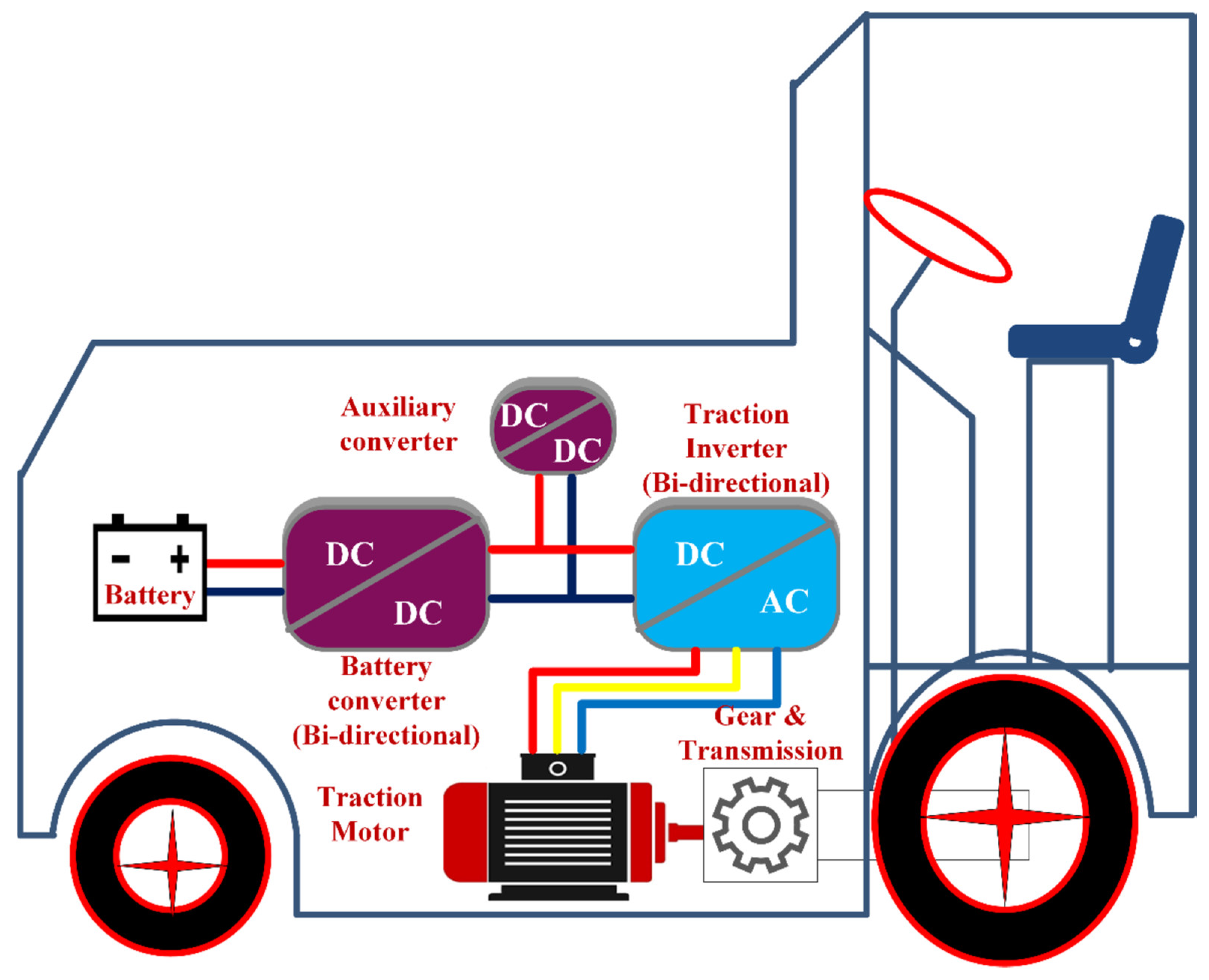
An electric tractor’s propulsion system consists of a motor, a power electronic converter, and a controller. The motor drive system is the fundamental and most widely used technology in electric tractors (ETs) [1]. In a full electric tractor, the conventional drivetrain is eliminated. It is fully powered by electricity, and it will operate with all the benefits of an electric motor [2]. Figure 1 shows the complete drivetrain system used in ETs. The biggest disadvantage of a full electric tractor is that it requires a larger-capacity battery to achieve a decent range. Another disadvantage is that the electric powertrain is a bit more expensive [3]. However, it can be cheaper in the future owing to its development in production. With overwhelming battery developments, the ICE tractors will lose their importance. The savings in maintenance can also be substantial. In essence, a hydrogen fuel cell tractor (FCT) is an electric battery tractor with a range extender [4]. As a result, comparing it to an electric tractor is oversimplified. It also offers a few distinct advantages over a battery-powered tractor. A smaller battery is required. With enough space for hydrogen tanks and the ability to quickly recharge hydrogen, it can operate over a long distance. The issue is that natural gas is used to make 90% of the hydrogen; therefore, there is no reduction in emissions [5]. Even if the hydrogen is produced in a sustainable manner, the efficiency is much lower. The features of different hybridization configurations are compared in

Table 1. Features of topology configuration of different tractors [6].

Features		ICET	ET	HET	PHET	FCET
Energy storage		Fuel tank	Battery Ultra-capacitor	Fuel tank Battery Ultra-capacitor	Fuel tank Battery Ultra-capacitor	Fuel cell Battery Ultra-capacitor
Energy source		Petrol/diesel	Electric energy	Petrol/diesel and electric energy	Petrol/diesel and electric energy	Hydrogen
Energy source Infrastructure		Refueling station	Charging station	Refueling station	Refueling station and charging station	Hydrogen refinery
Propulsion system		ICE	Electric motor	ICE and electric motor	ICE and electric motor	Electric motor
Efficiency	Well–tank	88.00%	37.00%	88.00%	-	58.4%
	Tank–wheel	12.1%	83.00%	22.3%	-	46.6%
	Well–wheel	10.6%	31.3%	19.6%	-	27.2%
Smooth operation		No	Yes	Yes	Yes	Yes
Emission		Very high	Zero	Low	Very low	Ultra-low
System complexity		Very low	Low	Moderate	High	Very high

.

The most critical attributes of an ET’s motor are its potential to provide adjustable driving control, high efficiency, high fault-tolerance, and low noise. Additionally, a rapid torque control is required to fulfil the driver-commanded instantaneous torque [7,8,9,10]. The permanent magnet synchronous motor (PMSM) is the best candidate for the ET drive system when used as the primary drive system in ETs. This is mostly because of its inherent advantages, which include compact in size and weight, a wide range of operating speeds, high torque-to-weight ratio, high power density, and more efficiency. By employing the proper torque management, it meets the tractor requirements [11,12].

Several torque control strategies are presented in the literature, which include field-oriented control (FOC) and direct torque control (DTC) [12,13,14,15]. These control techniques provide a wider range of options for motor control. Though it is possible to control torque and flux independently to achieve at least as good a dynamic performance through these methods, the limitations such as difficulty in controlling flux or torque at low speed, variable switching frequency, and insufficient control of DC current have limited the application of these control approaches. To maximize driving range on a single charge, ET must be highly efficient. This can be accomplished by minimizing losses, which is at the basis of the MTPA technique. Various MTPA-based torque control techniques are available for PMSM drives [16,17]. To begin with, a lookup table (LUT) strategy is employed to find the correlation between the torque and currents in the d, q-axes. Lookup tables are unable to account for the variation in machine characteristics caused by magnetic saturation effects. As a result, the LUT solution often does not achieve the MTPA criteria when the parameters fluctuate. Another possibility is to incrementally determine the optimal stator current value corresponding to the torque [18]. This can be achieved by using the mathematical formulation (which is carried out using the motor model) to estimate the optimal value of the stator current from the required reference torque. It provides an easy-to-implement solution. Additionally, it is a parameter-insensitive approach, as motor parameter variations can readily be incorporated into the formulas. As a result, this research employs it.

In high-performance drives, the desired reference speed should always be maintained, even with the load changes, saturation, and speed variations. Traditional controllers (P, PI, and PID) require a proper modeling of the control system that accurately describes the dynamics of the system. Additionally, designing such controllers without an adequate system model is a tremendously difficult task, and they require rigorous fine-tuning and are independent of system parameter change. Additionally, their performance is impacted by noise, temperature, saturation, and unpredictable load dynamics [19,20]. Model-predictive control (MPC) has recently attracted considerable attention as a potential alternative control strategy. The MPC approach predicts the future state values using a discrete motor model. Then, for each sampling period, the ideal voltage vector is derived by optimizing an operational cost function. One of the distinct advantages of the MPC over other controllers used in the literature, such as PI and PID controllers, is that it is capable enough in managing a wide variety of constraints. The MPC is employed in the multi-input and multi-output (MIMO) systems but the existing controllers are only applicable for the single-input and single-output (SISO) systems, which is regarded as a significant difference between the proposed and existing controllers. It is inherent in model-predictive control to handle the dynamic relationship between feedforwards and decoupling, but the existing controllers are not capable enough to do so. An inverter applies the specified ideal output voltages to the motor based on the cost function parameters [9,21,22]. The prime advantage of the MPC is to provide greater flexibility and intuition, since it achieves control objectives through the application of a mathematical cost function. Various system constraints and optimization are easily accomplished with the cost function [23,24]. Thus, the cost function can be used to account for torque and current magnitude limitations.

The purpose of this study is to demonstrate the IPMSM drive’s steady state and dynamic performance under varied load conditions. IPMSM is a suitable contender for high-speed applications due to its prominent pole structure and ability to utilize maximum torque with the lowest current levels. MPC with MTPA is presented for IPMSM to calculate ideal voltage vectors regardless of optimal switching sequence, which helps to decrease torque ripple and harmonic distortion, hence increasing the motor drive’s overall efficiency. FCS–MPC makes use of the motor drive’s discrete-time internal model to forecast the future state across a discrete sample time. The phase voltages are calculated using the voltage source inverter (VSI) switching states. The best voltage vector across the motor drive is chosen in accordance with a cost-function-defined control target.

This paper is organized as follows: mathematical modeling of the system, including electric tractor, IPMSM, and MTPA, is presented in Section 2. Field working conditions and load cycle considered for the duty calculation of ET are explained in Section 3, and the MPC–MTPA algorithm is presented in Section 4. In Section 5, HIL implementation is described. Simulation and experimental results are presented in Section 6.

2. Mathematical Modeling

2.1. Modeling of Electric Tractor

The dynamic operation of an electric tractor is described with the help of Newton’s law of motion. When the tractor is operating in the field, it requires a very high torque. During the tractor operation, there are a number of forces acting on it [25]. The forces that act on the tractor are taken into consideration while performing the calculations for power and torque requirements, which are shown in Figure 2. The tractor motion can be determined by analyzing the forces acting on it, in the direction of motion.

The force required to propel the tractor along with the implements attached to it is known to be tractive force (F_tr), which is given by Equation (1) [26]:

$$F_{tr}=F_{roll}+F_{air}+F_{grade}+F_{acc}+F_{drawbar}$$

(1)

where $F_{roll}$ is rolling resistance force, $F_{air}$ is aerodynamic drag force, $F_{grade}$ is grading resistance force, $F_{acc}$ is acceleration force, and $F_{drawbar}$ is the implement draft force.

During farming applications, a tractor will operate in fields with a farming implement connected to it. $F_{drawbar}$ is the force required to drive the implement in the direction of tractor movement. Draft force is necessary to pull various seeding implements and some tillage tools at shallow depths. It is essentially determined by the width of the farm implement and the velocity at which it is dragged. Draft is further affected by soil texture, depth, and farming tool geometry when using tillage implements at deeper depths. Draft force is calculated based on standards provided by the American Society of Agricultural and Biological Engineers (ASABE) standards [27].

$$F_{drawbar}=F_i\times \left[A+B\left(v\right)+C{\left(v\right)}^2\right]\times W\times T$$

(2)

where F is the soil texture adjustment parameter (dimensionless). For fine-textured soil, i = 1, 2 for medium, and 3 for coarse-textured soils. A, B, and C are the machine-specific parameters, v is the operating velocity of tractor (in km/h), W is machine width (in meters) or number of rows, and T is tillage depth (in centimeters) for major tools. T is taken as 1 (dimensionless) for minor tools and seeding implements.

Due to the friction between the tire and the soil, the tractor experiences rolling resistance force. When the tractor is traveling at a particular velocity, it has to overcome the resistance offered by the air. While the tractor is moving in an uphill direction, it has to overcome additional resistance forces caused due to the gradient of the road. Although the tractor overcomes all the resistive forces, it requires an acceleration force to propel it in the desirable direction. All these forces are given in Equations (3)–(6) [26].

$$F_{roll}=M·g·C_{rr}·cos\alpha$$

(3)

$$F_{air}=\frac{1}{2}\rho C_d{A}_f{v}^2$$

(4)

$$F_{grade}=M·g·sin\alpha$$

(5)

$$F_{acc}=\delta M\frac{dv}{dt}$$

(6)

By substituting Equations (2)–(6) into Equation (1), the total tractive force at the wheels of the tractor is

$$F_{tr}=M·g·C_{rr}·cos\alpha +\frac{1}{2}\rho C_d{A}_f{v}^2+M·g·sin\alpha +\delta M\frac{dv}{dt}+\left[F_i\times \left[A+B\left(v\right)+C{\left(v\right)}^2\right]\times W\times T\right]$$

(7)

For tractor trailer mode,

$$F_{tr}=M_{eff} g\left(sin\alpha +C_{r}cos\alpha \right)+\frac{1}{2}\rho C_d{A}_f{v}^2+\delta M_{eff}\frac{dv}{dt}$$

(8)

$$M_{eff}=W_{tractor}+W_{trailer}$$

$$F_{tr}=M_{eff} g\left(sin\alpha +C_{r}cos\alpha \right)+\frac{1}{2}\rho C_d{A}_f{v}^2+\left(M_{eff}+J{\left(\frac{n_g}{R_w}\right)}^2{\eta }_{tr}\right)\frac{dv}{dt}$$

(9)

where J refers the inertia of the transmission system. Instantaneous torque at tractor wheel $T_w$ is a product of tractive force and driving wheel radius ($T_w=F_{ta}\times r$).

$$T_{tr}=R_w\left[M_{eff} g\left(sin\alpha +C_{r}cos\alpha \right)+\frac{1}{2}\rho C_d{A}_f{v}^2+\left(M_{eff}+J{\left(\frac{n_g}{R_w}\right)}^2{\eta }_{tr}\right)\frac{dv}{dt}\right]$$

(10)

In BET, the electric motor transfers the torque via the transmission system (fixed gear) to the wheels. The electromagnetic torque $T_{em}$ is

$$T_{sh}=\frac{R_w}{{\eta }_{tr}{n}_g}\left[M_{eff} g\left(sin\alpha +C_{r}cos\alpha \right)+\frac{1}{2}\rho C_d{A}_f{v}^2+\left(M_{eff}+J{\left(\frac{n_g}{R_w}\right)}^2{\eta }_{tr}\right)\frac{dv}{dt}\right]$$

(11)

$$T_{sh}=\frac{R_w}{{\eta }_{tr}{n}_g}\left[M_{eff} g\left(sin\alpha +C_{r}cos\alpha \right)+\frac{1}{2}\rho C_d{A}_f{v}^2\right]+\frac{R_w}{{\eta }_{tr}{n}_g}\left[\left(M_{eff}+J{\left(\frac{n_g}{R_w}\right)}^2{\eta }_{tr}\right)\frac{dv}{dt}\right]$$

(12)

$$T_{sh}=\frac{R_w}{{\eta }_{tr}{n}_g}\left[M_{eff} g\left(sin\alpha +C_{r}cos\alpha \right)+\frac{1}{2}\rho C_d{A}_f{v}^2\right]+M_{eq}\frac{d}{dt}v$$

(13)

$$M_{eq}=\left(\left(\frac{R_w}{{\eta }_{tr}{n}_g}\right)M_{eff}+J\left(\frac{n_g}{R_w}\right)\right)$$

For input drive cycle, the reference velocity v with required acceleration, the load torque at the motor shaft is given as

$$v=\left(\frac{R_w}{n_g}\right)w$$

$$T_l=\frac{R_w}{{\eta }_{tr}{n}_g}\left[M_{eff} g\left(sin\alpha +C_{r}cos\alpha \right)+\frac{1}{2}\rho C_d{A}_f{\left(\frac{R_w}{n_g}\right)}^2{w}^2\right]+J_{eq}\frac{dw}{dt}$$

(14)

$$J_{eq}=J+\left(\frac{R_w{}^2}{{\eta }_{tr}{n}_g{}^2}\right)M_{eff}$$

2.2. Modeling of PMSM

Mathematical modeling of the PMSM is essential for its control. The controller is designed based on the mathematical model of the machine. In most cases, the PMSM is modeled in the d–q reference frame to avoid the dependency of motor coefficients on rotor position. In the d–q reference frame, the stator voltages of PMSM are as follows [28].

$$v_d=i_d·R_s+\frac{d{\lambda }_d}{dt}-w_e{L}_q{i}_q$$

(15)

$$v_q=i_q·R_s+\frac{d{\lambda }_q}{dt}+w_e{L}_d{i}_d+w_e{\lambda }_{pm}$$

(16)

Flux linkages are

$${\lambda }_d=L_d·i_d+{\lambda }_{pm}$$

(17)

$${\lambda }_q=L_q·i_q$$

(18)

Substituting the equations into the above equation,

$$v_d=i_d·R_s+L_d\frac{d{i}_d}{dt}-w_e{L}_q{i}_q$$

(19)

$$v_q=i_q·R_s+L_q\frac{d{i}_q}{dt}+w_e{L}_d{i}_d+w_e{\lambda }_{pm}$$

(20)

Electromagnetic torque produced is

$$T_e=\frac{3}{2}p\left[{\lambda }_{pm}{i}_q\left(L_d-L_q\right)i_d{i}_q\right]$$

(21)

$$T_e-T_L=J\frac{d{w}_m}{dt}+B{w}_m$$

(22)

$$w_e=\frac{P}{2}{w}_m$$

where v is the voltage, L is the inductance, i is the current, R_s is the stator resistance, w is the rotor speed, ${\lambda }_{pm}$ is the flux linkages, suffixes d, q indicate the d-axis and q-axis components, respectively, e and m indicate electrical and mechanical values, and pm indicates the permanent magnet. A block diagram of PMSM mathematical modeling is shown in Figure 3. Torque Equation (21) consists of two terms; the first one is electromagnetic torque due to the permanent magnetic flux of the rotor, and the second one is reluctance torque, which is due to the saliency of the rotor.

2.3. MTPA Modeling

The structure of the IPMSM is salient in nature; due to this, it is not easy to achieve MTPA control by using the q-axis current controller. If the d-axis current is kept to zero, as speed increases the stator voltage increases, and the current controller reaches saturation at high speeds for a given reference torque. This phenomenon results in drive instability of the IPMSM. When i_d = 0, the IPMSM produces only electromagnetic torque, which is directly proportional to q-axis current, and the reluctance torque is completely absent. This results in inaccuracy of IPMSM control, since the full capacity of the IPMSM is not utilized to generate the torque for various operations. To utilize the advantage of saliency in the IPMSM, the magnitude of the stator current is being fixed along the dq axis, and a current limit circle can be drawn, which is depicted in Figure 4a. As illustrated, the MTPA trajectory (tangential to current circle) is drawn by varying the current from zero to its maximum value.

From the phasor diagram of the PMSM, which is shown in Figure 4b, the dq axis currents in terms of torque angle are [28]:

$$i_q=I_s sin\beta$$

(23)

$$i_d=I_s cos\beta$$

(24)

By substituting (23) and (24) into (21), the torque equation becomes

$$T_e=\frac{3}{2}\frac{P}{2}\left[{\lambda }_{pm}{I}_s sin\beta +\left(L_d-L_q\right)I_s{}^2 sin\beta cos\beta \right]$$

(25)

$$T_e=\frac{3}{2}\frac{P}{2}\left[{\lambda }_{pm} I_s sin\beta +\left(L_d-L_q\right)I_s{}^2\frac{sin2\beta }{2}\right]$$

(26)

To obtain the MTPA, we differentiate the torque Equation (26) with torque angle and equate to zero:

$$\frac{d{T}_e}{d\beta }=0$$

$${\lambda }_{pm} \left(I_s cos\beta \right)+\left(L_d-L_q\right)\left({\left(I_s cos\beta \right)}^2{\left(I_s sin\beta \right)}^2\right)=0$$

(27)

$${\lambda }_{pm} i_d+\left(L_d-L_q\right)\left(i_d{}^2-i_q{}^2\right)=0$$

(28)

Finally, $i_d$ corresponding to MTPA is

$$i_d=\frac{{\lambda }_{pm} \pm \sqrt{Lmd{a}^2+8{\left(L_d-L_q\right)}^2{I}_s{}^2}}{4\left(L_d-L_q\right)}$$

(29)

The value of $i_d$ cannot be positive; if it is positive, the core reaches saturation. Hence, the final value of $i_d$ corresponding to MTPA is

$$i_d=\frac{{\lambda }_{pm}-\sqrt{Lmd{a}^2+8{\left(L_d-L_q\right)}^2{I}_s{}^2}}{4\left(L_d-L_q\right)}$$

(30)

The stator current $I_s$ is

$$I_s=\sqrt{i_d{}^2+i_q{}^2}$$

(31)

From (31), $i_q$ is

$$i_q=\sqrt{I_s{}^2-i_d{}^2}$$

(32)

The MTPA algorithm optimizes the stator current to deliver a possible amount of maximum torque. This results in reduction in stator copper loss and hence improves the efficiency. In addition to this, the MTPA algorithm is easy to design and execute and provides better dynamics under varying loads.

3. Farmland Working Conditions for the Load Calculations

For modeling and fixing the ratings of a traction motor, a field track with two conditions are considered. One is a continuous transfer ploughing operation (in between farmlands 1, 2, and 3), and the other is the soil deep loosening operation (farmland 4) illustrated in Figure 5. The distance covered at each turning is 10.5 m, and for entire farmlands are 105 m, 157.5 m, 220.5 m, and 220.5 m for farmlands 1, 2, 3, and 4, respectively. Figure 6 depicts the velocity vs. time graph for the operation of three farmlands. It consists of constant acceleration, constant velocity, constant deceleration, and turning stages, respectively. Before the start of the ploughing operation, the drive inputs the ploughing machine parameters mentioned in Table 1. In this study, the depth of operation is considered as 20 cm for farmlands 1, 2, and 3, and 30 cm for farmland 4. The required torque profile for the ploughing operation is shown in Figure 7. The RMS values of the torque are calculated from the figures.

4. MPC Control

The MPC approach outperforms traditional PI controllers in terms of dynamic performances and parameter tuning. At each sample time, the permissible switching patterns are listed, the relevant system response is estimated, the cost function is assessed, and the switching pattern with the minimum voltage vector is chosen. MPC is capable of dealing with multiple variables, which can be utilized to track the targeted dq current trajectory.

MPC uses the discrete model to forecast the future values of stator currents for possible combinations of each voltage vector. Over the sample period T_s, an internal discrete-time model of the IPMSM is utilized to forecast the future state of the output state variable, which is used to control the state input. The discrete model of IPMSM is derived as

$$\frac{d{i}_d\left(t\right)}{dt}=\frac{i_d\left(t_{i+1}\right)-i_d\left(t_i\right)}{T_s}$$

(33)

$$\frac{d{i}_q\left(t\right)}{dt}=\frac{i_q\left(t_{i+1}\right)-i_q\left(t_i\right)}{T_s}$$

(34)

To obtain the minimum possible voltage vector, the two-level voltage source inverter (VSI) is modeled using the equation, and the switching states of the VSI are given in

Table 2. Two-level VSI switching states and corresponding voltage vectors.

Sa	Sb	Sc	Voltage Vector (V)
0	0	0	$V_0=0$
1	0	0	$V_1=\frac{2}{3}{V}_{dc}$
1	1	0	$V_2=\frac{1}{3}{V}_{dc}+j\frac{\sqrt{3}}{3}{V}_{dc}$
0	1	0	$V_3=-\frac{1}{3}{V}_{dc}+j\frac{\sqrt{3}}{3}{V}_{dc}$
0	1	1	$V_4=-\frac{2}{3}{V}_{dc}$
0	0	1	$V_5=-\frac{1}{3}{V}_{dc}-j\frac{\sqrt{3}}{3}{V}_{dc}$
1	0	1	$V_6=\frac{1}{3}{V}_{dc}-j\frac{\sqrt{3}}{3}{V}_{dc}$
1	1	1	$V_7=0$

.

The phase voltages in the dq reference frame are given in Equation (35).

$$\left[\begin{array}{c}{v}_d\\ v_q\end{array}\right]=\frac{2}{3}{V}_{dc}\left[\begin{array}{cccccccc}0& cos\theta & cos\left(\theta -\frac{2\pi }{3}\right)& cos\left(\theta -\frac{4\pi }{3}\right)& -cos\theta & -cos\left(\theta -\frac{2\pi }{3}\right)& -cos\left(\theta -\frac{4\pi }{3}\right)& 0\\ 0& -sin\theta & -sin\left(\theta -\frac{2\pi }{3}\right)& -sin\left(\theta -\frac{4\pi }{3}\right)& sin\theta & sin\left(\theta -\frac{2\pi }{3}\right)& sin\left(\theta -\frac{4\pi }{3}\right)& 0\end{array}\right]$$

(35)

To calculate the predicted values of stator currents, physical modeling of the PMSM is required. The differential equations of stator currents are derived from Equations (19) and (20).

$$\frac{d{i}_d\left(t\right)}{dt}=\frac{1}{L_d}\left[v_d\left(t\right)-i_d\left(t\right)R_s+\omega \left(t\right)L_q{i}_q\left(t\right)\right]$$

(36)

$$\frac{d{i}_q\left(t\right)}{dt}=\frac{1}{Lq}\left[v_q\left(t\right)-i_q\left(t\right)R_s+\omega \left(t\right)L_d{i}_d\left(t\right)-\omega \left(t\right){\lambda }_{pm}\right]$$

(37)

By considering the sampling interval as T_s, at sampling time t_i, the future predicted values of stator currents are

$$i_d\left(t_{i+1}\right)=i_d\left(t_i\right)+T_s\frac{d{i}_d\left(t\right)}{dt}$$

(38)

$$i_q\left(t_{i+1}\right)=i_q\left(t_i\right)+T_s\frac{d{i}_q\left(t\right)}{dt}$$

(39)

By substituting in the above equations,

$$i_d\left(t_{i+1}\right)=i_d\left(t_i\right)+\frac{T_s}{L_d}\left[v_d\left(t_i\right)-i_d\left(t_i\right)R_s+\omega \left(t_i\right)L_q{i}_q\left(t_i\right)\right]$$

(40)

$$i_q\left(t_{i+1}\right)=i_q\left(t_i\right)+\frac{T_s}{L_q}\left[v_q\left(t_i\right)-i_q\left(t_i\right)R_s+\omega \left(t_i\right)L_d{i}_d\left(t\right)-\omega \left(t_i\right){\lambda }_{pm}\right]$$

(41)

Equations (40) and (41) can be rewritten as

$$i_d\left(t_{i+1}\right)=\left(1-\frac{R_s{T}_s}{L_d}\right)i_d\left(t_i\right)+\frac{T_s}{L_d}\left[v_d\left(t_i\right)+\omega \left(t_i\right)L_q{i}_q\left(t_i\right)\right]$$

(42)

$$i_q\left(t_{i+1}\right)=\left(1-\frac{R_s{T}_s}{L_q}\right)i_q\left(t_i\right)+\frac{T_s}{L_q}\left[v_q\left(t_i\right)-\omega \left(t_i\right)L_d{i}_d\left(t_i\right)-\omega \left(t_i\right){\lambda }_{pm}\right]$$

(43)

$i_{dq}\left(t_i\right)$ are the present state variables at sampling time $\left(t_i\right)$, and $i_{dq}\left(t_{i+1}\right)$ are the predicted future state variables at sampling time $\left(t_{i+1}\right)$. $v_{dq}\left(t_i\right)$ is the input variable, which is chosen using the switching state of the inverter.

Figure 8 illustrates the FCS–MPC design for the IPMSM. To obtain the minimum voltage vector, the selection of the cost function is necessary. In the proposed MPC, the inverter always tracks the reference currents and measured currents precisely. Figure 9 shows the flow diagram of the MPC. The cost function is described as [24]:

$$J={\left(i_{dref}\left(t_i\right)-i_d\left(t_{i+1}\right)\right)}^2+{\left(i_{qref}\left(t_i\right)-i_q\left(t_{i+1}\right)\right)}^2$$

(44)

By substituting (42) and (43) in (44), the cost function J is

$$\begin{gathered} J={\left(i_{dref}\left(t_i\right)-(1-\frac{R_s{T}_s}{L_d})i_d(t_i)+\frac{T_s}{L_d}[v_d(t_i)+\omega (t_i)L_q{i}_q(t_i)]\right)}^2+{(i_{qref}(t_i)-(1-\frac{R_s{T}_s}{L_q})i_q(t_i)+ \\ \frac{T_s}{L_q}\left[v_q(t_i)-\omega (t_i)L_d{i}_d(t_i)-\omega (t_i){\lambda }_{pm}\right])}^2 \end{gathered}$$

(45)

In the steady state, the cost function of the proposed FCS–MPC ensures the minimum number of switches changes. To generate the reference values of $i_{dqref}\left(t_i\right)$, the MTPA algorithm is used. There are seven pairs of $v_d\left(t_i\right)$ and $v_q\left(t_i\right)$ that are available at the sampling time $\left(t_i\right)$. According to the flow diagram, the very next step is to identify the pair of input parameters that minimizes the cost function J given in Equation (45). After obtaining optimal cost function index, the switching states are applied to VSI at the sampling time $\left(t_i\right)$. This results in the corresponding voltage, which is given in Table 1. If the determined cost function index is zero, the previous states of the VSI must be verified to decide if the index 0 or 7 should be applied in the control action. At the time $t=t_i+T_s$, the predicted values of stator currents $i_d\left(t_{i+1}\right)$, $i_q\left(t_{i+1}\right)$ and velocity $\omega \left(t_{i+1}\right)$ are updated. This results in seven new pairs of voltages $v_d\left(t_{i+1}\right)$, $v_q\left(t_{i+1}\right)$ that are calculated with angle $\theta \left(t_{i+1}\right)$. The cost function equation is updated with the new variable and it is minimized. A new optimal value of the cost function and its index at time $t=t_i+T_s$ generates the switching signals to the VSI.

Though it is already used in the existing approaches, the ideology of FS-MPC used in this present work is highly optimal compared to others because it is employed for the on-road electric vehicle applications in the conventional works but it is utilized for off-road applications in the operation of electric tractors in this present work, which is significantly considered as one of the major novelties of this proposed work. Moreover, this algorithm is modeled in such a way that it receives the commands of the driver and responds to those commands automatically, even in non-flattened agricultural surfaces, by considering many more dynamics, which is not considered in the existing works. The computational complexity is thus widely minimized with the assistance of this methodology, which in turn involves maximizing the overall performance of the entire system. Therefore, the presented work has novelty in the view of applications used that differ from the other conventional works.

5. HIL Implementation

The proposed model of the PMSM load characteristics for electric tractor application is verified using the HIL simulator OP5700, RT– LAB, programmable control board (PCB-E06-0560), MSOx3014T, and probes. The PCB is used to communicate between both the simulation and real controller using analog outputs and digital inputs. The configuration of the real—time implementation setup is depicted in Figure 10. HIL systems are frequently utilized for real-time simulations of engineering systems before implementing the prototyping tests. Stacks are capable of rapidly creating and synchronizing prototypes. The plant and controller are placed in OPALRT to enable the system to operate at real-time clock speeds. This process can be considered as a real-time system simulation, due to high-speed nanosecond to microsecond OPAL– RT sampling rate. The user’s personal computer is used to execute the RT-digital LAB’s simulator commands. RT– LAB is used to edit, build, load, and execute the prototype. The requirements and specifications of the HIL stack are given in

Table 3. Specifications of HIL stack.

Device Name	OP5700
FPGA	Xilinx Vertex 7 FPGA on VC707 board, 485T, 485, 760 Logic cells, 2800 DSP slices
I/O lines	256 lines, 8 analogue or digital, 16 or 32 channels
High-speed communication ports	16 SFP sockets, up to 5 Gbps
I/O connectors	4 panels of 4 DB37F connectors
Monitoring connectors	4 panels of RJ45 connectors
PC interface	Standard PC connectors (monitor, keyboard, mouse, and network)
Power supply	Input: 100–240 VAC, 50–60 Hz, 8 A–4 A. Power: 600 W

.

6. Result and Discussion

Simulation and experimental results of the proposed MPC–MTPA control for different speeds under variable load conditions are discussed here. The parameters of the IPMSM used in this work are listed in

Table 4. Parameters of the IPMSM.

Parameter	Value (Units)
Stator resistance (Rs)	0.0065 (ohm)
d-axis inductance (Ld)	1.597 (mH)
q-axis inductance (Lq)	2.057 (mH)
Trated	80 (Nm)
Nrated	1200 (rpm)
$\mathrm{Flux} \mathrm{linkages} ({\lambda }_{pm}$)	0.1757
Pole pairs	4
Vdc	560 (V)
Inertia (Jm)	0.09 (kg·m2)
Friction coefficient (Bm)	0.002 (Nms)

. The results are presented in two different regions. First, one is control of the IPMSM in constant torque region and second one is control of the PMSM in both constant torque and constant power regions. In the first case, simulation run time is 1 s and the IPMSM will operate in the base speed region; for this, the MPC–MTPA is implemented. In the second case, the simulation run time is also 1 s and the IPMSM will operate in the base speed region until 0.7 s. After 0.7 s, the IPMSM will operate in flux-weakening mode with maximum speed and reduced torque. At time t = 1 s, the IPMSM reference torque (T_ref) will become negative and it will produce negative torque.

6.1. Case 1

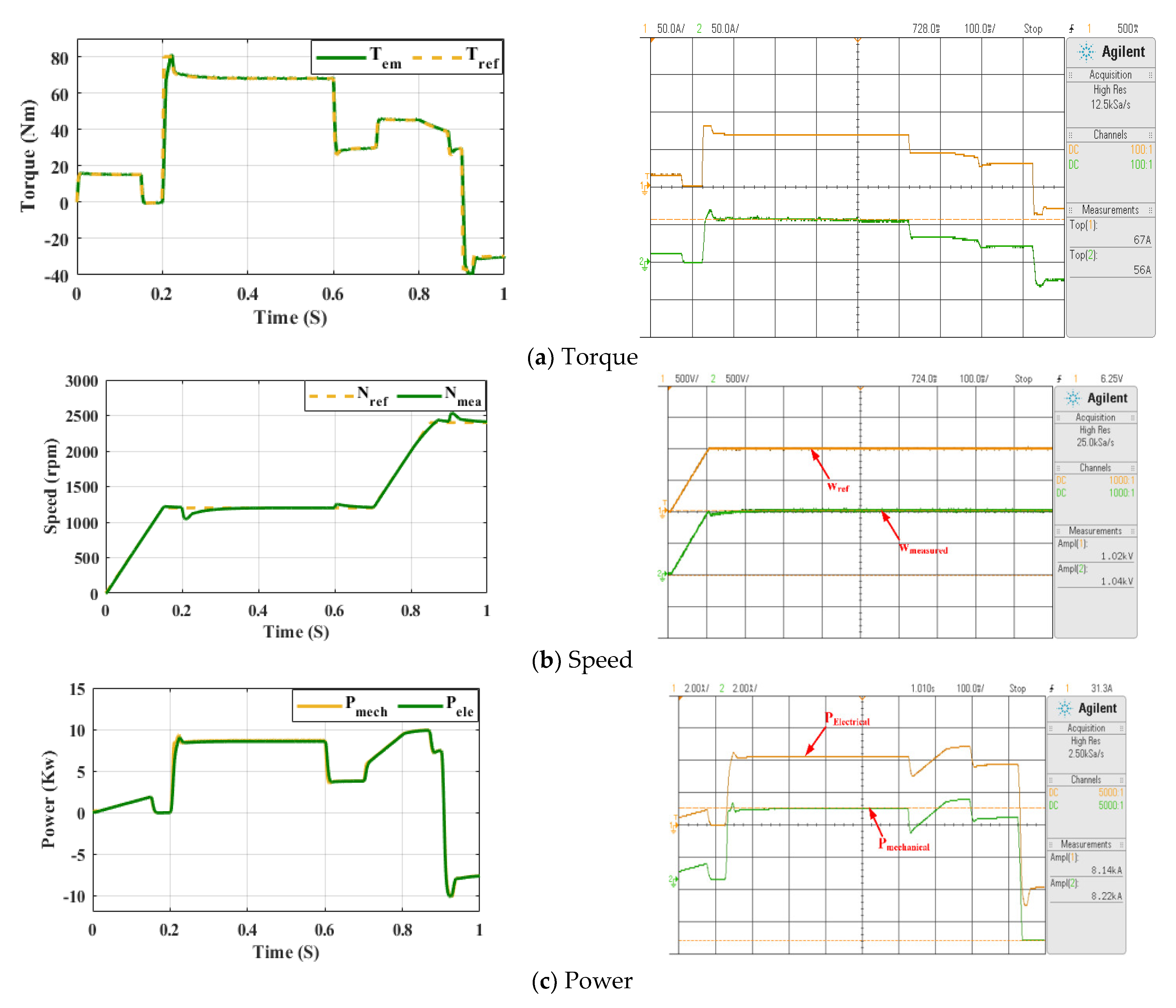
In this case, the motor starts accelerating at a slew rate of 10,000 and reaches 1000 rpm at t = 0.1 s; while accelerating, the motor requires a torque of 20 Nm. Once the motor speed reaches steady state, it operates at 70 Nm and the same torque is maintained until t = 1 s torque. Speed responses are shown in Figure 11a,b. During time t = 0.5 s to 0.85 s, MTPA control is activated. At this time, the current drawn from the motor is reduced and, at the same time, there is no change in the motor torque.

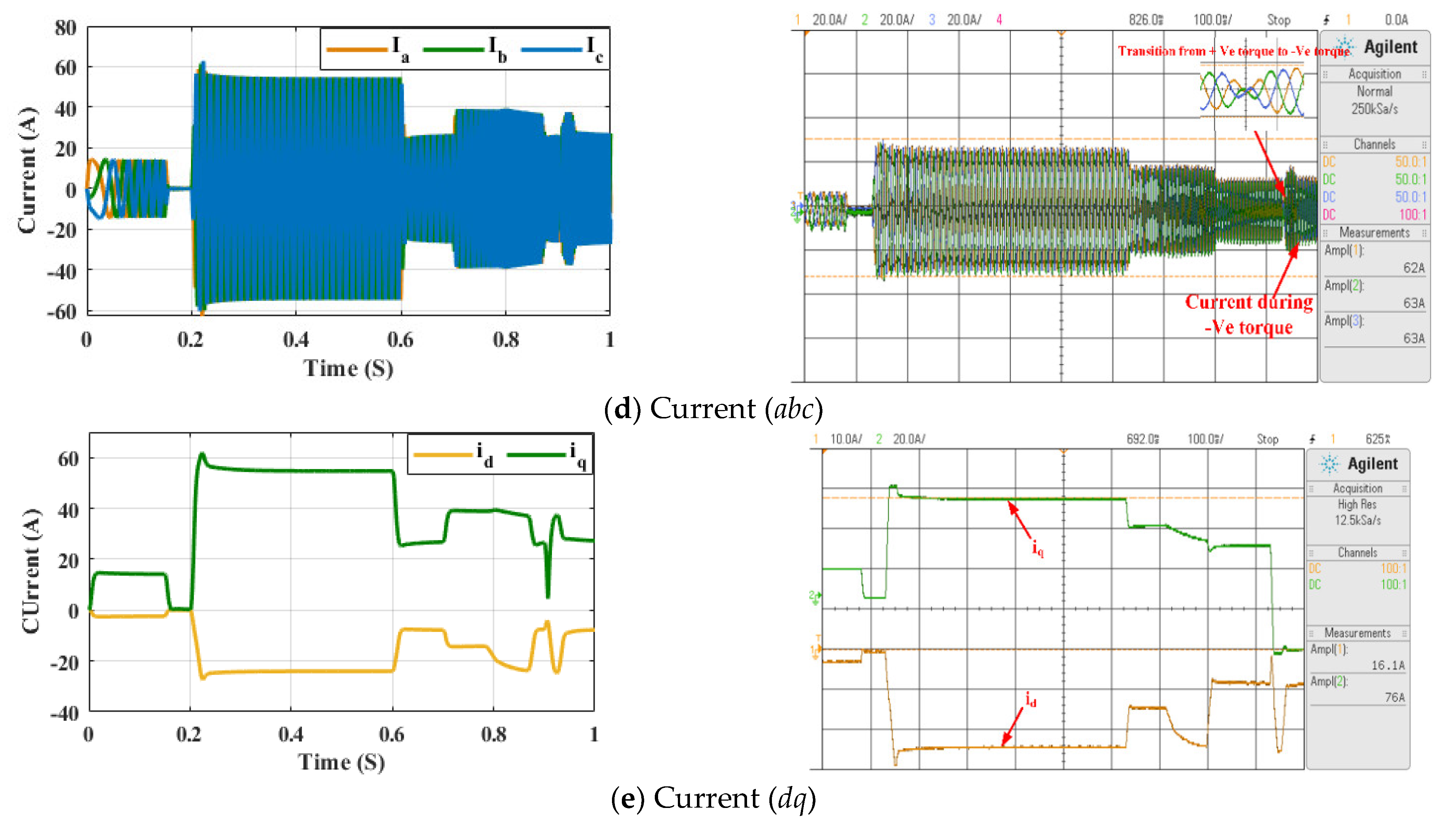
The current waveform is shown in the figure. At t = 0.85 s, MTPA control is turned off, and again the stator current increases. Reduction in the value of the stator current during MTPA control is shown in the zoomed-in figure. The MTPA is on and off at t = 0.5 s and 0.85 s, respectively, and there is a small dip in the electromagnetic torque produced. It is clearly shown zoomed-in in Figure 11a. Figure 11c shows the input electrical power and the output mechanical power produced. During MTPA control, the difference between these powers are reduced; hence, the losses are reduced during MTPA control. Finally, Figure 11d,e show the abc and dq axis current response. The d-axis current reaches negative value at t = 0.5 s, and again it reaches zero at t = 0.85 s; this shows that the MTPA control is successfully simulated. When the d-axis current is negative, the magnitude of the q-axis current is reduced to maintain the optimal stator current value during the MTPA. The HIL results of torque, speed, power, and currents (abc and dq) are also shown in Figure 11.

6.2. Case 2

In case 2, the total simulation runtime is t = 1 s. The IPMSM operates at base speed, above base speed, and in generator mode. Similar to case 1, the motor starts accelerating at a slew rate of 8000 and reaches its base speed of 1200 rpm at 0.18 s. During this acceleration, the motor produces torque of 16 Nm. Once the motor reaches its base speed at t = 0.2 s, a torque of 70 Nm is applied and the motor continues to produce it. At t = 0.6 s, the torque is reduced to 35 Nm and the speed is the same, 1200 rpm, until 0.7 s. At t = 0.7 s, the motor accelerates at a slew rate of 8000 and reaches 2400 rpm at 0.88 s; this time, the motor operates above base speed. During the speed transition from base speed to overspeed (1200 to 2400 rpm), the motor produces more torque (40 Nm) than the applied torque (30 Nm). Once the motor reaches steady state again, the motor produces the same torque (30 Nm). At t = 0.9 s, the motor torque moves into negative and operates as a generator. During this, there is no change in the motor speed. The torque and speed responses for case 2 are depicted in Figure 12a,b respectively. Figure 12c,d show the power and current (abc) response for the above torque and speed requirements. The responses of the dq axis currents are shown in Figure 12e. The d-axis current is always negative since the motor operates in MTPA and overspeed operations. The HIL results of torque, speed, power, and currents are also shown in Figure 12.

The results show that the implemented MPC− MTPA works accurately.

Table 5. Comparison of current and loss reduction of the IMPSM with MTPA control.

Load	Current		Current Reduction (%)	Loss Reduction (%)
	Without MTPA	With MTPA
Full Load	85	69	16.47	34
3/4 Load	63.5	55	13.4	25
Half Load	42	38	9.5	18
1/4 Load	21.4	20.5	4.2	8

shows the reduction of current and reduction of power loss with MTPA control. By employing MTPA control when the IPMSM is operating at full load, the stator current is reduced by 16.47%, and similarly by 13%, 9.5%, and 4.2% at 3/4 load, half load, and 1/4 load, respectively. The percentage reductions in loss are 34%, 25%, 18%, and 8% at full load, ¾ load, half load, and ¼ load, respectively. While operating at full load, around one third of the stator copper loss is reduced. To achieve better efficiency from MTPA control, it is always preferable to operate the motor at full load or nearer to full load. The comparison of current with MTPA control of Different loads is represented in Figure 13.

7. Conclusions

The paper presents the highly efficient control of the IPMSM. Unlike conventional methods, the suggested approach avoids the modulation block and maximizes torque by utilizing a minimum current constraint. The MPC is used to control power electronic switches logically. With an optimized control method, the motor drive’s speed response becomes rapid and robust under various load situations. The rapid dynamic reaction significantly reduces the steady-state error throughout the output of the motor drive. The IPMSM drive’s overall response is improved with the designed MPC. The MTPA method is the most effective while operating the motor at near full load conditions. Matlab/Simulink was used for developing the MPC–MTPA control. In addition, it was validated using the real-time HIL simulator. The results show the precision and robustness of the MPC–MTPA. The proposed control successfully reduced the stator loss and torque ripples and improved the motor drive’s efficiency and performance. The results show that the proposed MPC–MTPA improves the overall drive efficiency under variable loads.

In future, this study will be effectively implemented for the sensorless speed control. In addition, this work can be extended such that the speed control and current controllers can be combined as a single MPC to eliminate the cascaded connection in the controller such that it will produce more predominant speed and torque responses for the load changes.

References

- Nagar, H.; Shwetanshu; Bisaria, S.; Dalei, A.; Reddy, G.C.; Sultana, W.R.; Chitra, A. Powertrain Sizing and Performance Evaluation for Battery Electric Vehicle Using Model Based Design. In Proceedings of the 2021 Innovations in Power and Advanced Computing Technologies (i-PACT), Kuala Lumpur, Malaysia, 27–29 November 2021; IEEE: Piscataway, NJ, USA, 2021; pp. 1–6. [Google Scholar]
- Taha, Z.; Passarella, R.; Rahim, N.A.; Sah, J.M. Driving force characteristic and power consumption of 4.75 kW permanent magnet motor for a solar vehicle. J. Eng. Appl. Sci. 2010, 5, 26–31. [Google Scholar]
- Vogt, H.H.; de Melo, R.R.; Daher, S.; Schmuelling, B.; Antunes, F.L.M.; dos Santos, P.A.; Albiero, D. Electric tractor system for family farming: Increased autonomy and economic feasibility for an energy transition. J. Energy Storage 2021, 40, 102744. [Google Scholar] [CrossRef]
- Xun, Q.; Liu, Y.; Zhao, N. Energy Efficiency Comparison of Hybrid Powertrain Systems for Fuel-Cell-Based Electric Vehicles. In Proceedings of the 2020 IEEE Transportation Electrification Conference and Expo, ITEC, Chicago, IL, USA, 23–26 June 2020. [Google Scholar] [CrossRef]
- Ghobadpour, A.; Mousazadeh, H.; Kelouwani, S.; Malvajerdi, A.S.; Rafiee, S. Design, development, and evaluation of a PV_Bio-Gen range extender for an off-road electric vehicle. Int. J. Renew. Energy Res. 2020, 10, 388–399. [Google Scholar]
- Wang, B.; Xu, M.; Yang, L. Study on the economic and environmental benefits of different EV powertrain topologies. Energy Convers. Manag. 2014, 86, 916–926. [Google Scholar] [CrossRef]
- Dang, L.; Bernard, N.; Bracikowski, N.; Berthiau, G. Design Optimization with Flux Weakening of High-Speed PMSM for Electrical Vehicle Considering the Driving Cycle. IEEE Trans. Ind. Electron. 2017, 64, 9834–9843. [Google Scholar] [CrossRef]
- Zhang, Y.; Cao, W.; McLoone, S.; Morrow, J. Design and Flux-Weakening Control of an Interior Permanent Magnet Synchronous Motor for Electric Vehicles. IEEE Trans. Appl. Supercond. 2016, 26, 1–6. [Google Scholar] [CrossRef]
- Xie, W.; Wang, X.; Wang, F.; Xu, W.; Kennel, R.M.; Gerling, D.; Lorenz, R.D. Finite-Control-Set Model Predictive Torque Control with a Deadbeat Solution for PMSM Drives. IEEE Trans. Ind. Electron. 2015, 62, 5402–5410. [Google Scholar] [CrossRef]
- Nemeth, T.; Bubert, A.; Becker, J.N.; de Doncker, R.W.; Sauer, D.U. A Simulation Platform for Optimization of Electric Vehicles with Modular Drivetrain Topologies. IEEE Trans. Transp. Electrif. 2018, 4, 888–900. [Google Scholar] [CrossRef]
- Huang, S.; Wu, G.; Rong, F.; Zhang, C.; Huang, S.; Wu, Q. Novel Predictive Stator Flux Control Techniques for PMSM Drives. IEEE Trans. Power Electron. 2019, 34, 8916–8929. [Google Scholar] [CrossRef]
- Li, G.; Hu, J.; Li, Y.; Zhu, J. An Improved Model Predictive Direct Torque Control Strategy for Reducing Harmonic Currents and Torque Ripples of Five-Phase Permanent Magnet Synchronous Motors. IEEE Trans. Ind. Electron. 2019, 66, 5820–5829. [Google Scholar] [CrossRef]
- Morales-Caporal, R.; Leal-Lopez, M.E.; de Jesus Rangel-Magdaleno, J.; Sandre-Hernandez, O.; Cruz-Vega, I. Direct Torque Control of a PMSM-Drive for Electric Vehicle Applications. In Proceedings of the 2018 International Conference on Electronics, Communications and Computers (CONIELECOMP), Cholula, Mexico, 21–23 February 2018; IEEE: Piscataway, NJ, USA, 2018; Volume 2018, pp. 232–237. [Google Scholar]
- Shinohara, A.; Inoue, Y.; Morimoto, S.; Sanada, M. Maximum Torque Per Ampere Control in Stator Flux Linkage Synchronous Frame for DTC-Based PMSM Drives Without Using q-Axis Inductance. IEEE Trans. Ind. Appl. 2017, 53, 3663–3671. [Google Scholar] [CrossRef]
- Abassi, M.; Khlaief, A.; Saadaoui, O.; Chaari, A.; Boussak, M. Performance Analysis of FOC and DTC for PMSM Drives Using SVPWM Technique. In Proceedings of the 2015 16th International Conference on Sciences and Techniques of Automatic Control and Computer Engineering (STA), Monastir, Tunisia, 21–23 December 2016; pp. 228–233. [Google Scholar] [CrossRef]
- Liu, Q.; Hameyer, K. Torque Ripple Minimization for Direct Torque Control of PMSM With Modified FCSMPC. IEEE Trans. Ind. Appl. 2016, 52, 4855–4864. [Google Scholar] [CrossRef]
- Zhang, H.; Dou, M.; Deng, J. Loss-Minimization Strategy of Nonsinusoidal Back EMF PMSM in Multiple Synchronous Reference Frames. IEEE Trans. Power Electron. 2020, 35, 8335–8346. [Google Scholar] [CrossRef]
- Yang, R.; Sun, T.; Feng, W.; He, S.; Zhu, S.; Chen, X. Accurate online MTPA control of IPMSM considering derivative terms. Chin. J. Electr. Eng. 2021, 7, 100–110. [Google Scholar] [CrossRef]
- Sakunthala, S.; Kiranmayi, R.; Mandadi, P.N. Investigation of PI and Fuzzy Controllers for Speed Control of PMSM Motor Drive. In Proceedings of the 2018 International Conference on Recent Trends in Electrical, Control and Communication (RTECC), Malaysia, Malaysia, 20–22 March 2018; pp. 133–136. [Google Scholar] [CrossRef]
- Perera, A.; Nilsen, R. Gauss-Newton: A Prediction-Error-Gradient based Algorithm to Track PMSM Parameters Online. In Proceedings of the 2020 IEEE International Conference on Power Electronics, Drives and Energy Systems (PEDES), Jaipur, India, 16–19 December 2020; pp. 1–8. [Google Scholar] [CrossRef]
- Zhang, X.; Wang, K. Current Prediction Based Zero Sequence Current Suppression Strategy for the Semicontrolled Open-Winding PMSM Generation System with a Common DC Bus. IEEE Trans. Ind. Electron. 2018, 65, 6066–6076. [Google Scholar] [CrossRef]
- Razia Sultana, W.; Lodhi, A.; Gade, C.R.; Chitra, A.; Vanishree, J.; Manimozhi, M. Model Predictive Control of Quasi-Z-Source Inverter. In Lecture Notes in Electrical Engineering; Springer: Berlin/Heidelberg, Germany, 2021; Volume 700, pp. 3051–3062. ISBN 9789811582202. [Google Scholar]
- Murali, A.; Wahab, R.S.; Gade, C.S.R.; Annamalai, C.; Subramaniam, U. Assessing Finite Control Set Model Predictive Speed Controlled PMSM Performance for Deployment in Electric Vehicles. World Electr. Veh. J. 2021, 12, 41. [Google Scholar] [CrossRef]
- Cash, S.; Zhou, Q.; Olatunbosun, O.; Xu, H.; Davis, S.; Shaw, R. New traction motor sizing strategy for an HEV/EV based on an overcurrent-tolerant prediction model. IET Intell. Transp. Syst. 2019, 13, 168–174. [Google Scholar] [CrossRef]
- Ahmed, A.; Akl, M.; Rashad, E.E.M. A comparative dynamic analysis between model predictive torque control and field-oriented torque control of IM drives for electric vehicles. Int. Trans. Electr. Energy Syst. 2021, 31, e13089. [Google Scholar] [CrossRef]
- American Society of Agricultural and Biological Engineers. Test; ASABE: St. Joseph, MI, USA, 2011; p. 9. [Google Scholar]
- BOZTAŞ, G. Comparative Modelling and Experimental Verification of a PMSM Drive System. Eur. J. Tech. 2022, 12, 82–88. [Google Scholar] [CrossRef]
- Dianov, A.; Tinazzi, F.; Calligaro, S.; Bolognani, S. Review and Classification of MTPA Control Algorithms for Synchronous Motors. IEEE Trans. Power Electron. 2022, 37, 3990–4007. [Google Scholar] [CrossRef]
Figure 1.
Block diagram of an ET.
Figure 2.
Forces acting on a tractor.
Figure 3.
Representation of mathematical model of the PMSM.
Figure 4.
(a) Current circle and MTPA trajectory of the PMSM. (b) Phasor diagram of the PMSM for MTPA operation.
Figure 5.
Field track considered during the load calculation for the ploughing operation.
Figure 6.
Velocity vs. time graph of the ploughing operation.
Figure 7.
Torque profile for the ploughing operations.
Figure 8.
Block diagram of the proposed MPC−MTPA control.
Figure 9.
Flow diagram of MPC.
Figure 10.
Configuration of HIL implementation.
Figure 11.
Simulation and HIL results of (a) torque, (b) speed, (c) power, (d) current (abc), and (e) current (dq) for case 1.
Figure 12.
Simulation and HIL results of (a) torque, (b) speed, (c) power, (d) current (abc), and (e) current (dq) for case 2.
Figure 13.
Comparison of current for different loads with MTPA control.