
Energy Efficiency of Personal Computers: A Comparative Analysis
by
 , , , and
Beatriz Prieto
1,*,
Juan José Escobar
1,
Juan Carlos Gómez-López
1,
Antonio F. Díaz
1 and
Thomas Lampert
2 1
Department of Computer Architecture and Technology, CITIC, University of Granada, E-18071 Granada, Spain
2
ICube, University of Strasbourg, F-67081 Strasbourg, France
*
Author to whom correspondence should be addressed.
Sustainability 2022, 14(19), 12829; https://doi.org/10.3390/su141912829
Submission received: 25 July 2022
/
Revised: 14 September 2022
/
Accepted: 24 September 2022
/
Published: 8 October 2022
Abstract
:The demand for electricity related to Information and Communications Technologies is constantly growing and significantly contributes to the increase in global greenhouse gas emissions. To reduce this harmful growth, it is necessary to address this problem from different perspectives. Among these is changing the computing scale, such as migrating, if possible, algorithms and processes to the most energy efficient resources. In this context, this paper explores the possibility of running scientific and engineering programs on personal computers and compares the obtained power efficiency on these systems with that of mainframe computers and even supercomputers. Anecdotally, this paper also shows how the power efficiency obtained for the same workloads on personal computers is similar to that obtained on supercomputers included in the Green500 ranking.
1. Introduction
Currently, among the most important challenges of society is to reduce energy consumption in order to maintain or promote the sustainability of our planet. As an example of this challenge, the European Union (EU) aims to reduce greenhouse gas emissions by 40% by 2030 [1]. Energy, necessary for the vast majority of our activities, is also among the greatest sources of pollution. Energy production, supply, and consumption generate 75% of greenhouse gas emissions in Europe. The EU Green Deal sets the objective of making Europe climate neutral by 2050.
A report coordinated by Victor Zhirnov and published by the U.S. Semiconductor Industry Association, in collaboration with the Semiconductor Research Corporation (SRC) and the National Science Foundation (NFSF), states that while world energy production has grown linearly, the demand for electricity from computers has grown exponentially [2,3]. In typical situations, the lower-edge system-level energy required per one bit transition is considered to be approximately 10–14 joules, which is the estimate used for laptops and PCs as well as supercomputers [3,4]. Among the conclusions of the report is that, if this trend continues to increase, the electrical consumption of this vast amount of technological equipment could exceed the world’s electricity production by the year 2040 [5].
Other researchers estimate that, in the worst-case scenario, Information and Communications Technologies (ICTs) could contribute up to 23% of global greenhouse gas emissions in 2030 [6,7].
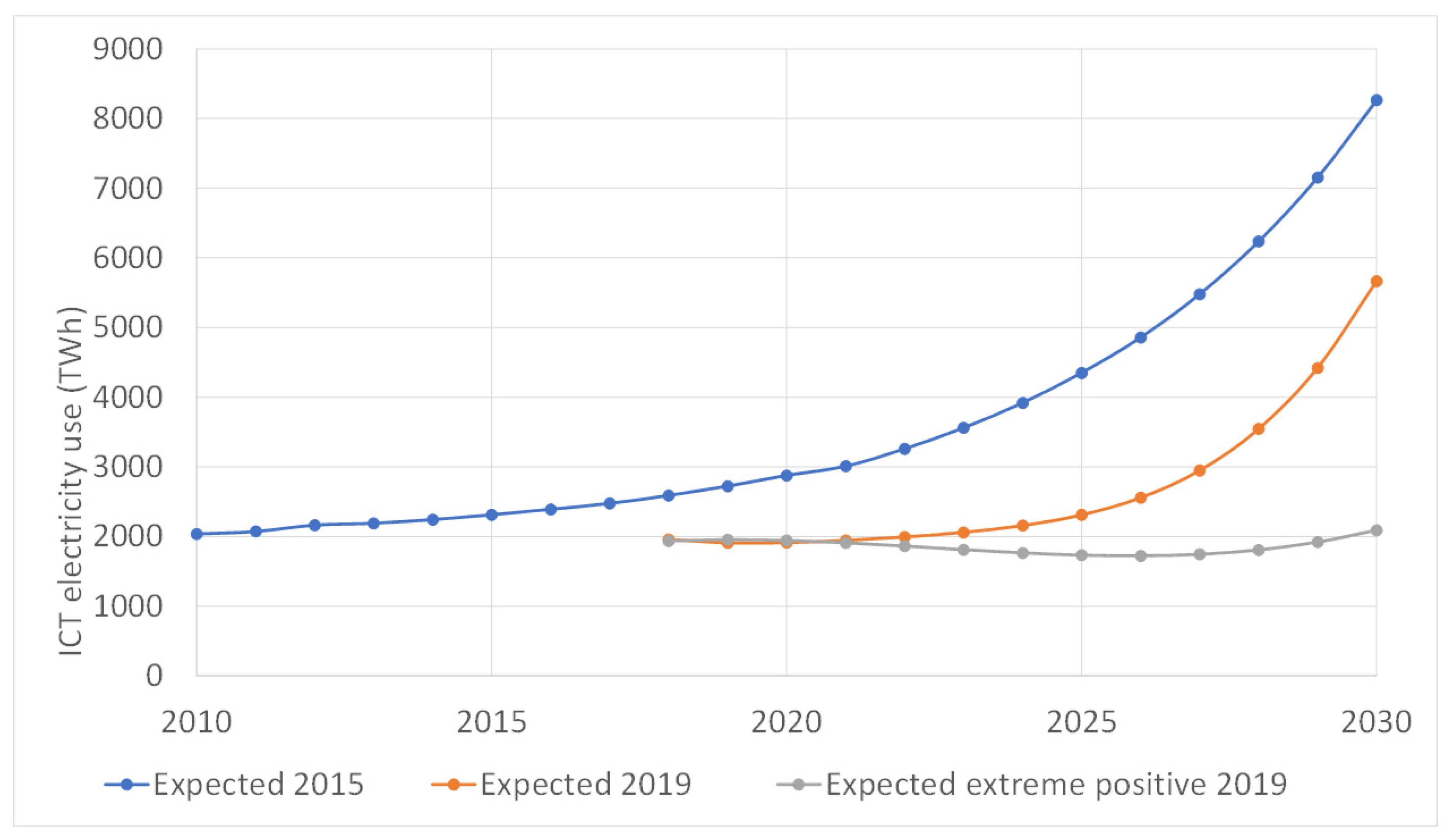
Most of the above forecasts and those included in other papers are not rigorous because they wrongly assume that energy consumption in the Internet of Things (IoT) sector grows proportionally with the number of devices, users or data traffic. Analyses carried out in the middle of the last decade concluded that the growth of energy consumption around 2010 in countries such as Sweden, Germany and the US [8,9,10,11,12] was decreasing. Additionally, Andrae and Edler analyzed and modelled the electric power use for ICTs in separate studies in 2015 [6] and 2019 [13]. Figure 1 shows the evolution of the energy consumed per year (TWh) calculated using data from those studies. It can be seen that the estimated consumption from 2019 to 2030 is lower than the results and expectations of 2015.
The reduced consumption growth can be due to the following actions, and can come close to being extremely successful (as shown in the figure) if they are taken [11,14]:
- Improvements in the management of systems and data centers aimed at optimizing energy efficiency. For example, an interesting way to reduce energy consumption in data centers is, as suggested in [15], to reduce the number of servers that are powered on to a minimum and switching unused servers off or to low power mode.
- Widespread adoption of more efficient technologies. An example of this is to change from Hard Disk Drive (HDD) to Solid State Drive (SDD) technology, which has enabled a significant reduction in the consumption of mass data storage. More efficient technologies are also sought to reduce the environmental impact from the design and manufacturing phases of ICT resources [16].
- Changes in scale. A clear example would be in the move from smaller to large data centers that could be called hyperscale centers (such as Google Cloud, Amazon Web Services, Microsoft Azure, OVHCloud, Rackspace Open Cloud, or Microsoft Azure). In larger centers, power consumption can be better managed. Among the most important factors in energy consumption in data centers is air conditioning, and it is cost-effective to relocate hyperscale centers to locations where climatic conditions are more favorable. For example, one of Google’s largest data centers is located in Finland, where, being a Nordic country (very cold), air conditioning costs are lower than in warmer countries. This center uses the icy seawater of the Gulf of Finland to completely cool all its facilities [17]. This concept also includes proposals for energy-autonomous data centers [18].
The concept of scaling is connected to computation offloading, according to which processes that require intensive computing tasks are transferred to an external platform, which can be from a hardware accelerator to a cluster, grid, or cloud system [19,20,21,22,23]. According to the thesis defended in the present work, the offloading of programs or applications should not be done to a platform that speeds up the application the most, but to one that has greater energy efficiency if it can also satisfy time requirements. Among these platforms, personal computers should be considered, as is done in this paper.
In relation to changes in scale, the proliferation of smartphones and small mobile devices also results in a reduction of energy consumption since each of them offers a multitude of functions and services that were previously carried out by independent consumer devices (calculators, telephones, alarm clocks, planners, etc.), and can now be performed by a simple device designed for optimal energy consumption [8].
There is even a trend ensuring that the proportion of use-stage electricity by consumer devices will decrease and be transferred to networks and data centers [6].
A distributed system can include computers ranging from high-performance mainframe, servers, personal computers, and processors to small nodes in a sensor network. There are works that suggest, in distributed systems, algorithms and processes should be migrated to the most energy efficient resources [18].
Among the resources available for computing are personal computers (PCs), which include laptops (notebooks), desktops and workstations. PCs have improved considerably in their processing power and can be, as discussed in this paper, competitive from an energy point of view with servers and even with high-performance mainframe computers on the Green500 ranking for the same workloads. There are programs that a few decades ago could only be run on servers or clusters, that can be now run on PCs and, although the execution time difference is still extraordinary, the energy efficiency is better.
It should also be considered that there are complex calculation problems that need to be executed on portable computers and it is interesting to analyze the behavior of these systems by relating their performance rate of execution with their energy consumption. An example of this situation is presented in some biomedical applications that need to be performed with mobile equipment, as is the case in genomics, where, for example, real-time Polymerase Chain Reaction (PCR) tests are frequently needed and are implemented on portable personal computers (PCs) [24,25,26].
This paper tries to analyze the energy efficiency of executing scientific-technical problems on personal computers, and compares it with that obtained on servers and large computers. The aim is to show how shifting the execution of scientific-technical applications to smaller computers, such as PCs, can contribute to the overall reduction of energy consumption.
There is a growing amount of work related to the energy efficiency and performance evaluation of computing systems, mainly focused on aspects related to scheduling and distribution of tasks in clusters [27,28,29,30,31], data centers, and systems in the cloud [32,33,34,35,36]. Unlike the works cited, in this paper the analysis focuses on measuring the energy consumption of personal computers, using the Linpack benchmark to evaluate performance. The use of Linpack allows direct comparison of the energy efficiency figures obtained with those of the GREEN500 ranking, which is the list of the 500 most powerful computers and servers in the world. This list is updated every six months [37].
In accordance with the aforementioned objectives, this section of this paper (Section 1) described the importance of reducing the energy consumption of computing systems and ICTs to achieve a sustainable world. The actions and ideas that are being developed to achieve this objective have also been outlined, among which is the migration of scientific-technical applications to personal computers whenever the time requirements of the applications allow it. Now that the context of the work and related works has been defined, in Section 2 the materials and methods are presented. This includes the description and justification of the reference application (Section 2.1), the energy consumption measurement tools used (Section 2.2), the platforms and processors under test (Section 2.3), and the methodology used to perform the experiments (Section 2.4). On the other hand, Section 3 shows the experimental results obtained, which are interpreted and discussed in Section 4. This paper ends with some conclusions in Section 5.
2. Materials and Methods
In this section, the reference application used to measure different execution parameters, including the performance rate of execution and the average power consumed, is first described (Section 2.1). Then, the energy consumption measurement tools used in this study are justified (Section 2.2). Additionally, the systems to be analyzed (SUT, Systems under Test) are examined in terms of their computing power and energy performance (Section 2.3). Finally, the methodology used to perform the experiments is described (Section 2.4).
2.1. Reference Application
Linpack, which is a benchmark traditionally used to evaluate computing speed, initially designed for supercomputer [38], is used as a reference application for the comparative study between the performance of the five systems. Linpack is a computer program that solves a dense system of linear equations (), it determines the amount of time to factor and solve the system, and converts that time into a computing performance rate and assesses the results with partial pivoting to ensure their accuracy.
The performance rate of execution, R, is given as millions of floating-point operations per second (Mflop/s, or, in short, MFlops). This measurement is carried out with addition or multiplication operations using 64 bit floating point data. The results are also given in multiples of MFlops: GFlops (billions of floating-point operations per second) and TFlops (trillions of floating-point operations per second).
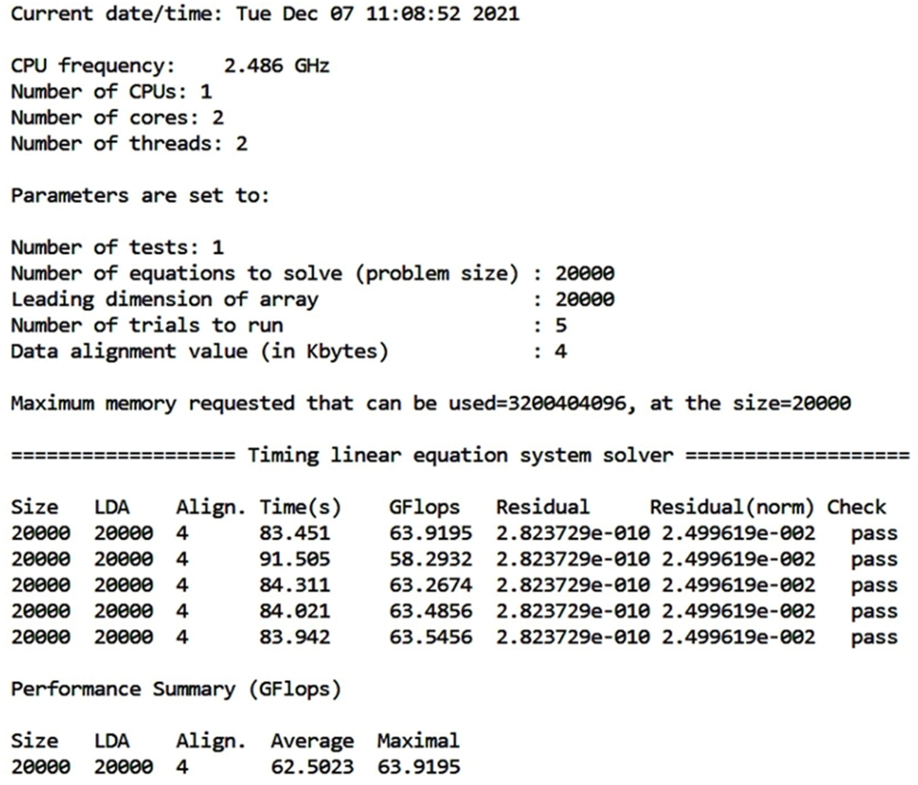
This work uses the Linpack Xtreme program released on Windows 10, 8, 7 (32 bit and 64 bit), version v1.1.5 of 31 December 2020 [39]. Linpack Xtreme is a console front-end developed by Intel with the Intel Math Kernel Library Benchmarks (2018.3.011) build of Linpack. Linpack Xtreme requires and generates the parameters shown in Table 1, and can be executed to solve:
- N = 15,000 linear equations (Quick, 2 GB benchmark),
- N = 20,000 linear equations (Standard, 2 GB benchmark) or
- N = 32,000 linear equations (Extended, 8 GB benchmark).
Figure 2 shows An example of a screenshot generated after a run of Linpack Xtreme.
2.2. Energy Consumption Measurement Tools
Within the Green Computing domain, among the main objectives is to obtain energy consumption models that allow the prediction and clear identification of each element’s contribution to the consumption of the system under study. The implementation of the models and predictions requires accurate measurements of the energy consumption in the systems to be modelled. These measurements can be made in the following ways:
- By using external power meters (wattmeters, ammeters, voltmeters) on the system, in series with the power cables to the wall outlet. With these external power meters, no granularity is obtained since only the overall power consumption of the system is measured, being, therefore, inadequate for a detailed analysis.
- By using separate metering hardware to be connected inside the system by the user. This additional hardware can include devices such as current sensors, current clamps, data acquisition cards, and microcontrollers. Measurements can be performed, for example, on the different DC power supply lines output from the system power supply, thus obtaining a certain degree of granularity. The cause of this behavior is due to the different lines supplying power to different parts of the computing system (motherboard, disk, etc.), although it is not possible to obtain measurements inside the chip.
- By using counters and hardware registers that are included as utilities or interfaces by the processor manufacturers for thermal and power management. With this type of interface, it is possible, for example, to develop tools to control the operation (ON/OFF) of fans or to monitor power consumption. An example is the RAPL (Running Average Power Limit) interface introduced by Intel in their Sandy Bridge processor architecture.
Both an external energy smart wattmeter (openZmeter) and a monitoring tool (Intel Power Gadget) based on the RAPL control register interface are used in this work. The openZmeter is used to measure global energy consumption in the SUTs, from which the energy efficiency is calculated (Section 3), while the Power Gadget allows to obtain separately the specific energy efficiency of the processors of the analyzed systems (Section 4). Furthermore, the simultaneous use of these two tools makes it possible to check the consistency between the measurements (waveforms, execution times, etc.) made with openZmeter and those made internally. Additionally, with the use of the Power Gadget, other collateral measurements to the objective of this work are obtained, such as RDTSC (number of cycles), elapsed time, CPU frequency, CPU utilization (%), and package temperature, which are included because they are related to the energy consumption of the complete equipment and can be analyzed in more detail in future works. These two tools are briefly described below.
2.2.1. OpenZmeter
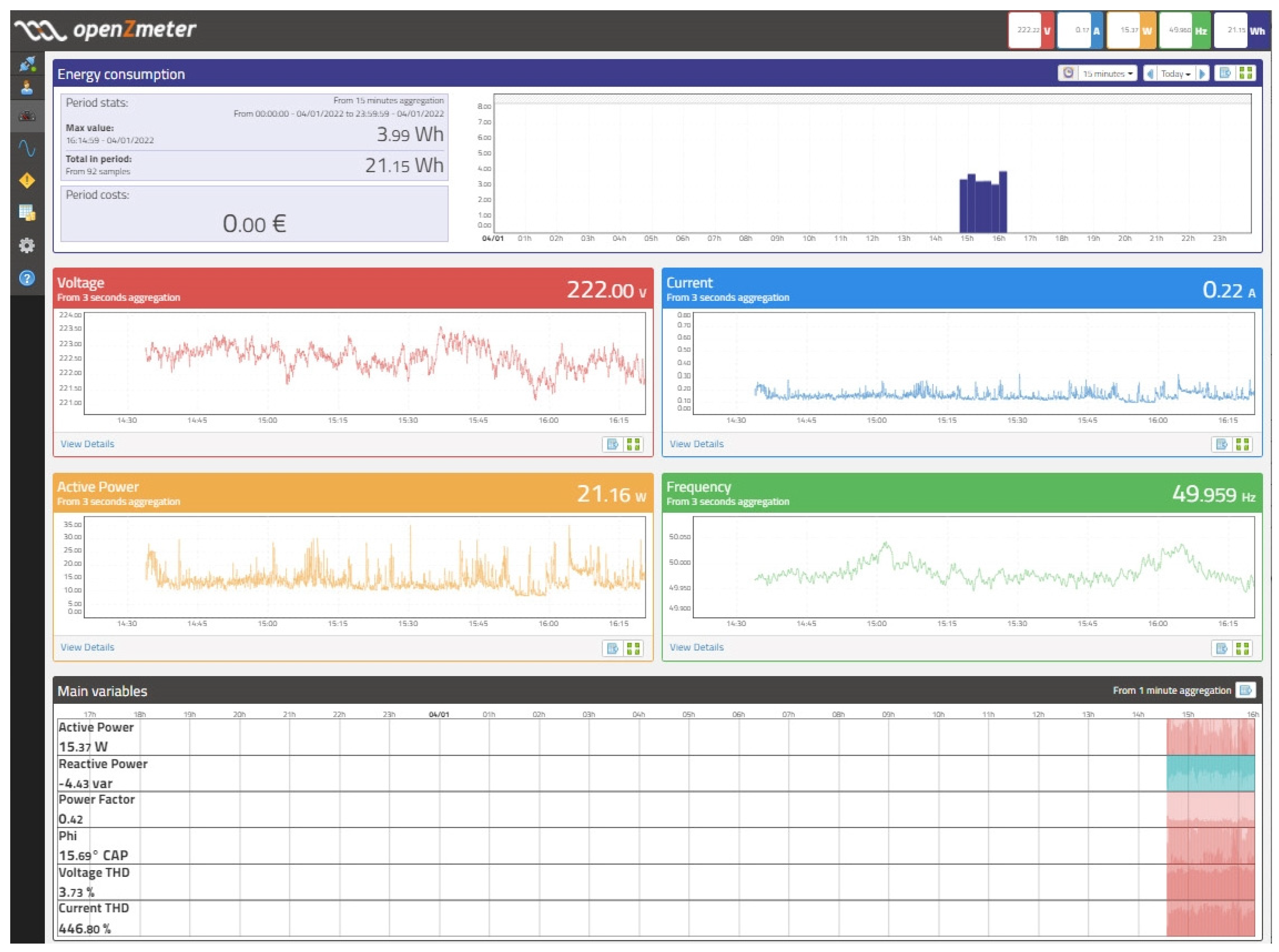
In the literature, there are several articles that have shown comparative studies about different smart energy meters [40]. In this research, the OpenZmeter (Figure 3) was used because it covers the requirements needed for the present work.
OpenZmeter (in short, oZm), is an efficient low-cost single and tri-phase smart electric energy meter described in [40]. The consumption pattern and power quality events are visualized through a user-friendly Supervisory Control and Data Acquisition (SCADA) tool. It also has an Application Programming Interface (API) for real-time query of all parameters that are displayed on the web interface itself.
The features of oZm that determined its selection are:
- Electrical measurements: Root Mean Square (RMS) voltage and current values; active, reactive, and apparent power and energy; power factor, harmonics, and frequency in real time through the API and stored in a database.
- Voltage measurement with a precision of 0.1% for RMS values. Frequency measurement with a precision of 10 MHz (in the range 42.5–57.5 Hz for 50 Hz power systems or 55.8–64.2 Hz). Current measurement up to 35 A RMS (integrated Hall-effect sensor).
- Sampling frequency of 15,625 Hz (64 microseconds between samples).
- Connectivity: USB ports (Wi-Fi dongle, 3G/LTE/4G, etc.), Ethernet port, and Wi-Fi. SPI, I2C, UART and PWM. Measurements can be visualized, for example, by accessing oZm via WiFi or the cloud via an MQTT-based synchronization service.
- Free and open system: Open-source software and hardware.
Data are stored in an SQL-like database (PostgreSQL) located in oZm and can be retrieved through the API at any moment. The computed data include time aggregations for minutes, day, week, month, or year. These data are analyzed with statistical tools [41] and the results can be then displayed to the user through a graphical interface specifically designed for oZm.
The main view (dashboard) of the oZm user interface (Figure 4) includes a summary of the main variables:
- The active energy consumption (kWh) for a fixed or variable time span (see top of Figure 4). Data can be shown in different time periods using aggregations based on nominal values of 3 s, 1 min, 10 min, or 1 h.
- Plots of RMS voltage, RMS current, frequency, and active power for a 3 s aggregation interval.
The measurements stored in the database can be analyzed in more detail by obtaining, for instance, average, maximum, and minimum magnitudes of voltage in a time period using different aggregation scales, and the voltage waveform. Table 2 shows an excerpt of a CSV file exported from oZm.
To a certain extent oZm, with its associated software, could be considered as a digital oscilloscope for waveform diagnosis. For more information, see [42].
2.2.2. Intel Power Gadget
The Intel Power Gadget tool uses the Running Average Power Limit (RAPL) interface, included by Intel in its Sandy Bridge processor architecture. RAPL is a tool that makes it possible to monitor and act on the processor’s power consumption and associated circuits. Indeed, RAPL allows the measurement of power consumption with a very fine granularity and a high sampling rate, and also makes it possible to limit the average power consumption of the different components inside the processor, which prevents the processor temperature from reaching an undesirable value [43]. With RAPL, it is possible to develop applications that capture real-time measurements of the power consumption of the CPU package and its components, as well as that of the DRAM memory managed by the CPU.
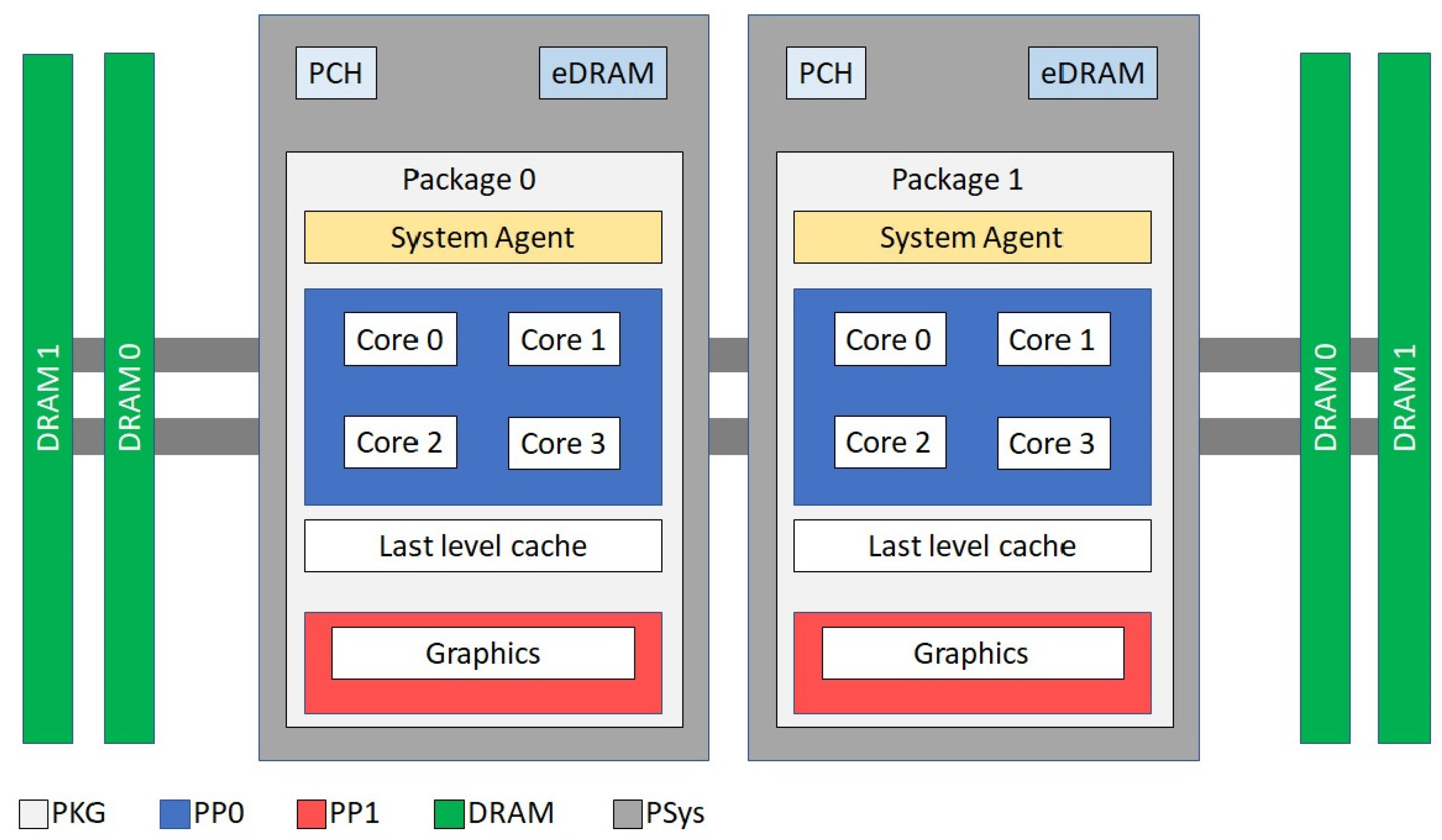
The RAPL interface provides this information through control register-counters (MSR, model-specific register) accessible from the instruction set included in the architecture specifically for debugging, program execution tracing, computer performance monitoring, and toggling/altering certain CPU features. Moreover, it considers different energy consumption zones or domains (Figure 5). Both monitoring and limiting energy consumption can be independently executed from each of the domains. These domains are the following [44]:
- Package (PKG). This domain includes the entire socket, i.e., of all cores and also the non-core components (L3 last level cache, memory controller, and integrated graphics).
- Power Plane 0 (PP0). This domain includes all processor cores on the socket.
- Power Plane 1 (PP1). This domain includes the graphics processor integrated on the socket (if it has one, as for example in desktop models).
- DRAM. Domain of the random-access memory (RAM) attached to the integrated memory controller.
- PSys. Domain available on some Intel architectures, to monitor and control the thermal and power specifications of the entire system on the chip (SoC), instead of just CPU or GPU. It includes the power consumption of the package domain, System Agent, PCH, eDRAM, and a few more domains on a single-socket SoC.
Not all architectures generate data from all the domains described above. For multi-socket server systems, each socket reports its own RAPL values.
The Intel Power Gadget is the other tool, in addition to oZm, used to perform the energy measurements in this work and is based on the use of the energy register-counters associated with the RAPL interface just described. This tool is enabled for Intel Core processors (from 2nd Generation up to 10th Generation) and is supported on Windows and Mac OS. It contains an application, driver, and libraries to monitor and estimate real-time processor package power information in watts (W) using the energy domain registers of the processor.
The Intel Power Gadget was chosen because:
- (1)
- It largely meets the needs for performing the measurements shown in Section 4,
- (2)
- It has been developed by the manufacturer of the processors under study,
- (3)
- It is freeware, and
- (4)
- It collects data from the RAPL interface.
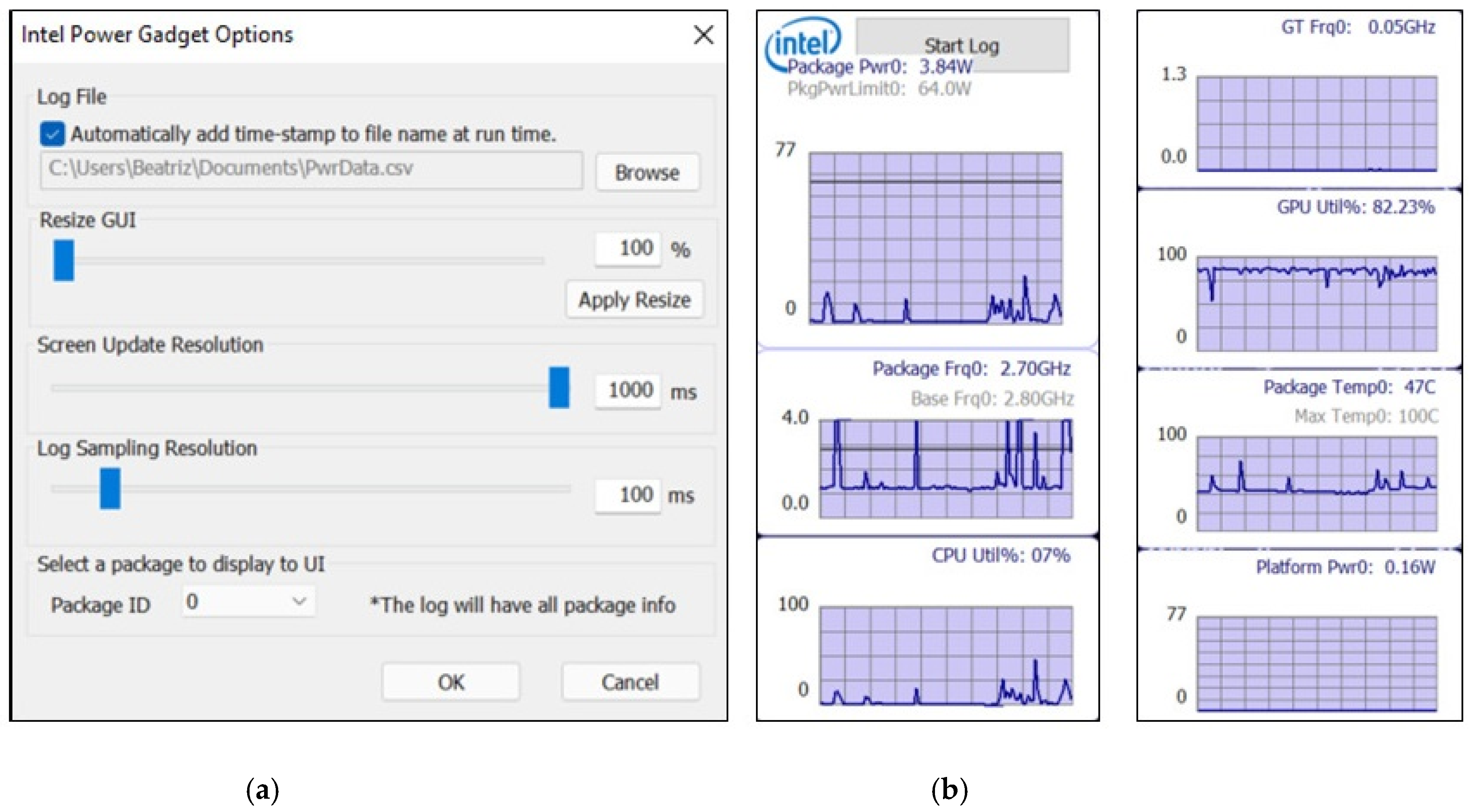
The in-depth study of the RAPL interface, using different benchmarks, implemented by K.N. Khan and M. Hirki [45] concludes that the RAPL readings are highly correlated with the socket power, sufficiently accurate and produce negligible performance overhead. Figure 6 shows graphs obtained during the execution of the Intel Power Gadget tool. An example of the data generated by Intel Power Gadget (once installed on the various test platforms) is shown in Table 3. The meaning of each of the parameters is provided in Table 4.
2.3. Platforms and Processors under Test
Table 5 shows the characteristics of the five systems under test (SUT). Four laptops and one desktop system (HP Pavilion) were selected, all of them with Windows OS. These computers belong to the authors’ research group at the University of Granada and were acquired over the years, so that the results provide an insight into the evolution of their performance over time.
Other characteristics of the processors can be found in [46]. TDP is the average power (watts, W) dissipated by the processor when operating at base frequency with all cores active under an Intel-defined, high-complexity workload; and TJunction is the maximum temperature allowed at the processor die.
2.4. Methodology
To analyze the performance rate when executing scientific problems and the energy efficiency of the computers under test, Linpack Extreme is run on each of the SUTs and, simultaneously, measurements with Intel Power Gadget and oZm are taken and stored. The information obtained is shown in Table 2 and Table 3.
The results generated in both applications are synchronized in time, and mean values, standard deviations, etc., are calculated. The time periods in which Linpack is being executed or not are also identified. To better interpret the results, the evolution of power consumption over time of the measurements obtained with Intel Power Gadget and oZm is also plotted.
To carry out the tests on each device, 5 runs of the Linpack Xtreme program are performed, which is the maximum value in the parameters established by Intel for each trial (see Table 1). It should be considered that the present work does not try to obtain exact values of the results but rather to qualitatively assess the adequacy of PCs from the energy point of view to execute scientific applications. Even so, the average and presented values are obtained, in the case of oZm, from more than 3 samples per second and, in the case of the Power Gadget, from 10 samples per second, which are sufficient for the required precision.
Measurements are performed without any additional air conditioning system, unlike with computers of a certain size that require expensive cooling equipment that consumes a large amount of energy, which should also be included in their measures.
The following section (Section 3) shows the results obtained after the above calculations.
3. Experimental Results
Table 6 summarizes the results obtained during the execution of Linpack on the five systems under test. First, the performance execution rate generated by Linpack Extreme are shown. Then, those obtained from the Intel Power Gadget outputs are displayed, and the table shows the average power in:
- The processor domain (UC + ALU + FPU + GT + other circuits on the chip)
- The IA domain (UC + ALU + FPU)
- The GT domain, and
- The DRAM domain.
It is worth mentioning that there are some subsystems from which no specific measurements are obtained, such as buses, disks, I/O ports, and internal cooling devices (fans). Finally, the average execution time and the average power consumption of five trials measured with oZm are included.
In each case, Linpack is run five consecutive times and the tables show the results of these five measurements. Linpack Extreme, Intel Power Gadget, and oZm data shown in the table correspond to the same five runs.
When the Linpack test is performed, it is obviously running in parallel to the OS and other system programs. In an attempt to obtain an estimate of the magnitudes specifically attributable to the execution of Linpack, an evaluation of the baseline (or idle) parameters has been performed. Here, we define the “core phases” [47] as the time intervals in which the Linpack program is running, and the “idle or baseline phases”, as those corresponding to intervals in which Linpack is not running, but in which the system is ready to start its execution. It should be noted that idle phases are not a state of suspension or hibernation.
The power consumed and other parameters in the idle phases have been estimated by averaging the values obtained in the time intervals where the program was not running, either before or after execution of a run of the five trials. These average values are considered system constants or reference values when the workload under analysis is not being executed.
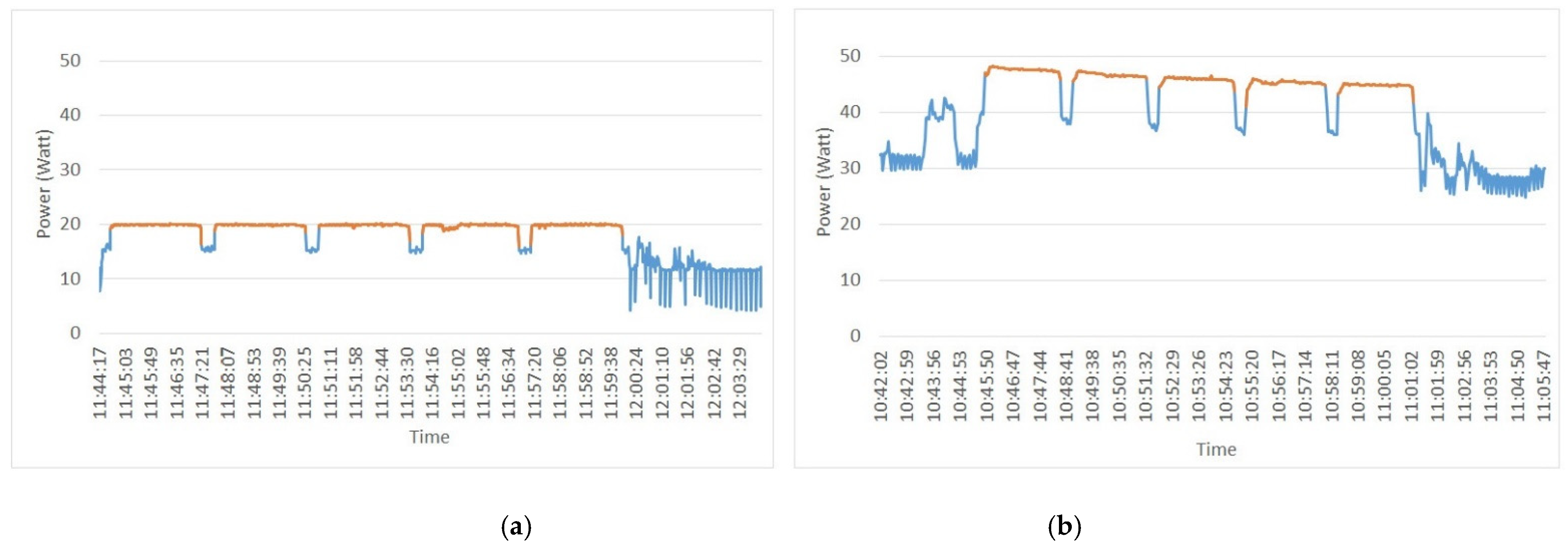
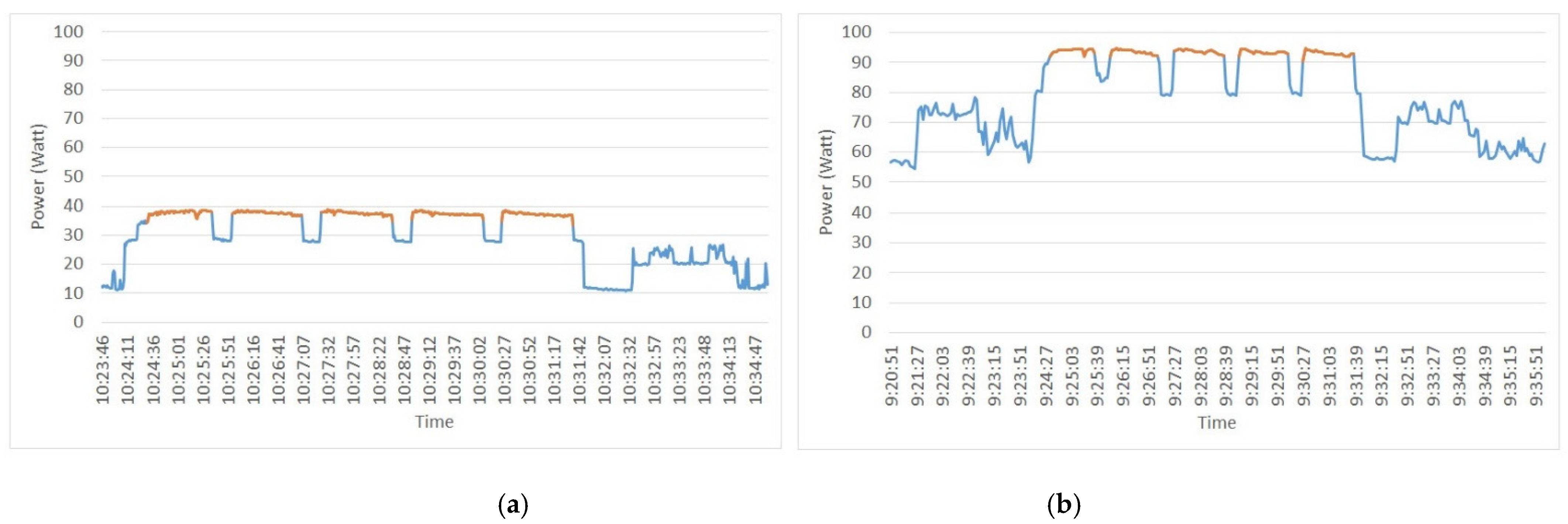
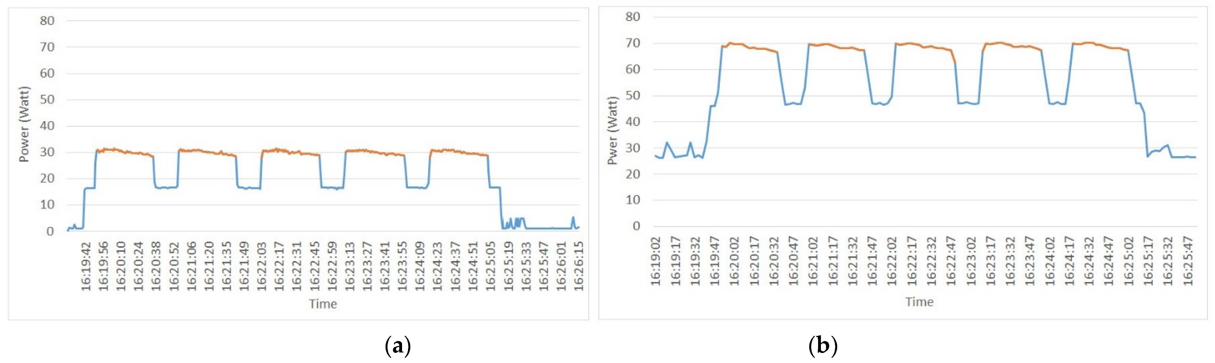
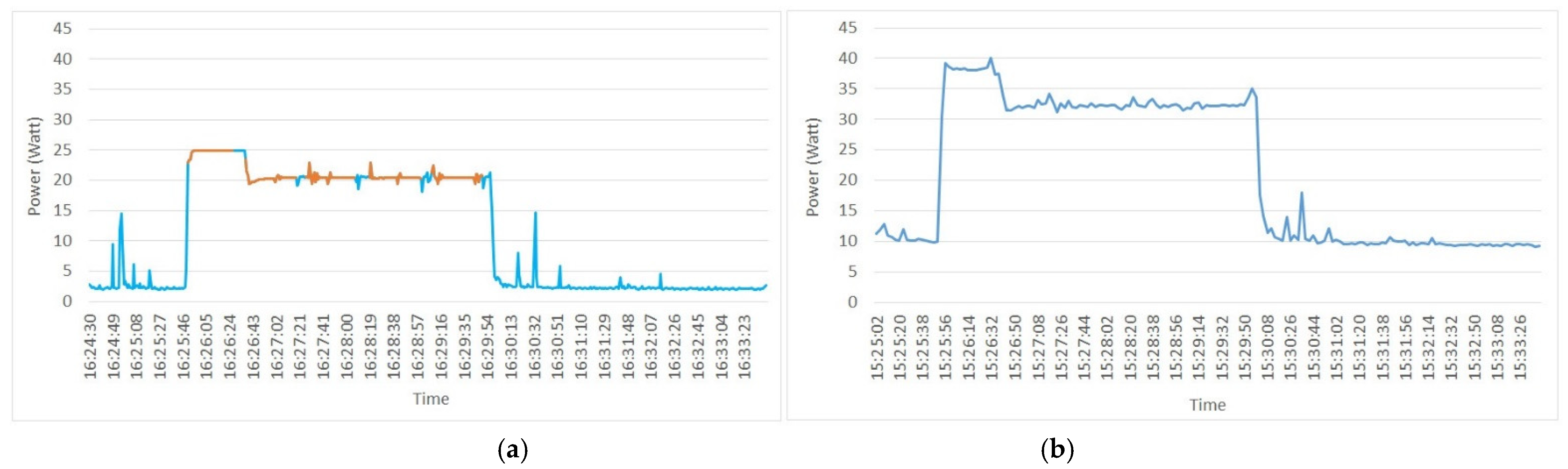
Considering the previous criteria, Table 7, Table 8, Table 9, Table 10 and Table 11 and Figure 7, Figure 8, Figure 9, Figure 10 and Figure 11 show the estimated values attributable to the Linpack executions, as well as the consumed power graphs obtained by both Intel Power Gadget and openZmeter. In the plots, the core phases are shown in orange, while the rest of the measurements correspond to the idle phases.
4. Discussion
Power efficiency (PE) is used to compare energy consumption in relation to power as it has become widely used in the community and in particular in the Green500 ranking. Green500 is a biannual list that ranks the supercomputers included in the TOP500 according to their energy efficiency [37,48].
Power efficiency is determined by obtaining the quotient between Linpack’s maximal performance rate of execution (Rmax) and average power (Paver) readings taken during such a run (the core phase of the run); including the power of the interconnection subsystem participating in the workload, i.e., the idle power. All in all, the power efficiency represents the performance rate per watt (Flops per Watt), that is:
The measurements of power or energy are typically made in Green500 at multiple locations in parallel across the computer system. Such locations can be, for example, at the entrance to each separate rack, or at the output connector of multiple building transformers [49].
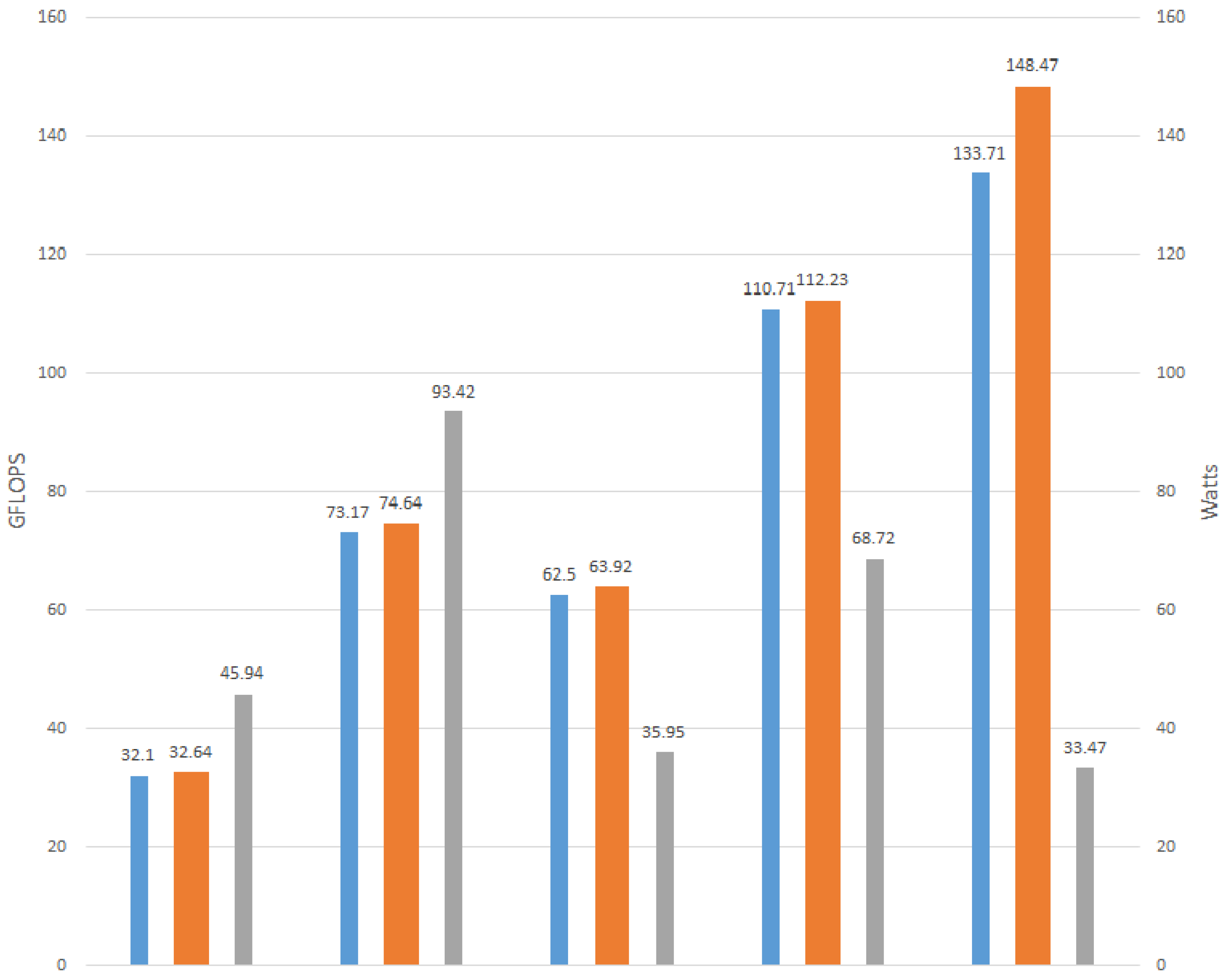
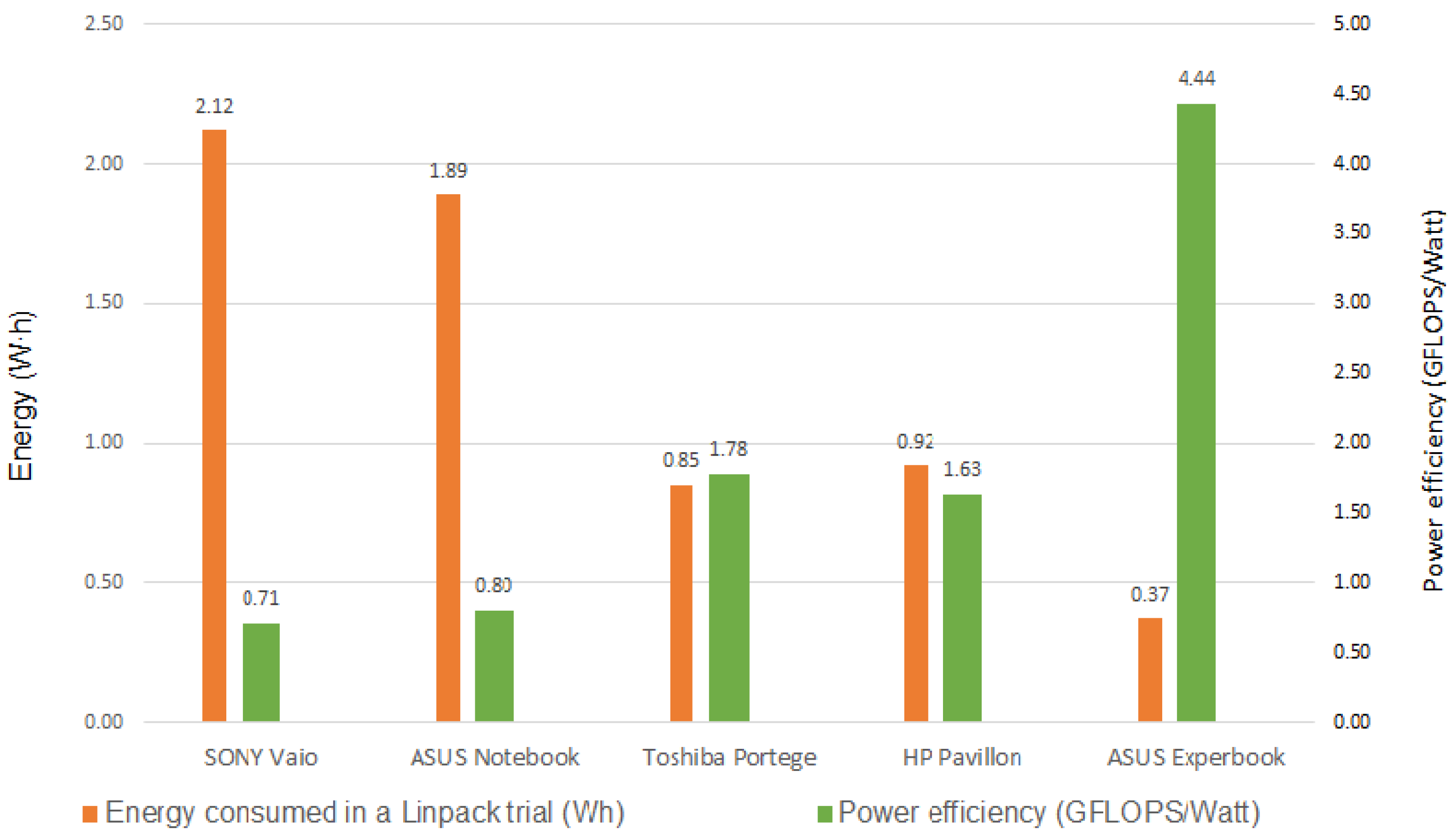
For the energy efficiency measurements of the systems under test in this work, similarly to Green500, we use the value generated with the Linpack runs as Rmax and the average power of all the electrical supply delivery to operate the computer system. That is, of the one obtained by oZm. Figure 12 and Figure 13 show the previous results in bar charts. As it can be seen, the most recent generations of equipment show a higher performance rate.
Note that the power consumed (W) by the processors does not depend directly on their performance rate, as might seem intuitive. Keep in mind that the power consumed depends on various factors, such as the density of the microprocessor’s transistors, whose growth has been determined by Moore’s Law. In this context, Dennard scaling holds, which states that if the density of the transistors is doubled, the power consumption stays approximately the same. Combining this property with Moore’s Law, it can be stated that over time the number of transistors in a dense integrated circuit (IC) doubles about every 24 months while the performance per watt does so approximately every 17 months. This forecast is no longer being fulfilled since transistors are reaching an atomic size for which the traditional physics models are no longer valid. As stated in [50], “transistors are still getting faster generation-to-generation but not at the same rate than what used to be achieved in the 90s, since the major emphasis in transistor design has now shifted from speed to limiting power consumption.”
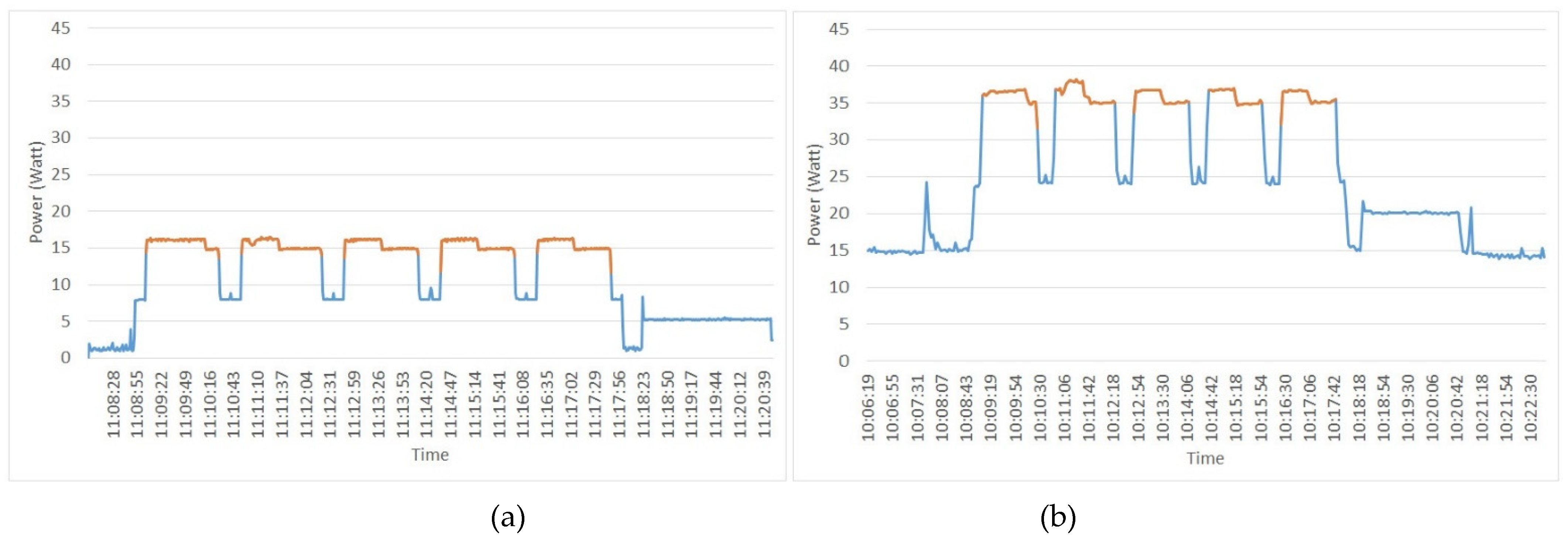
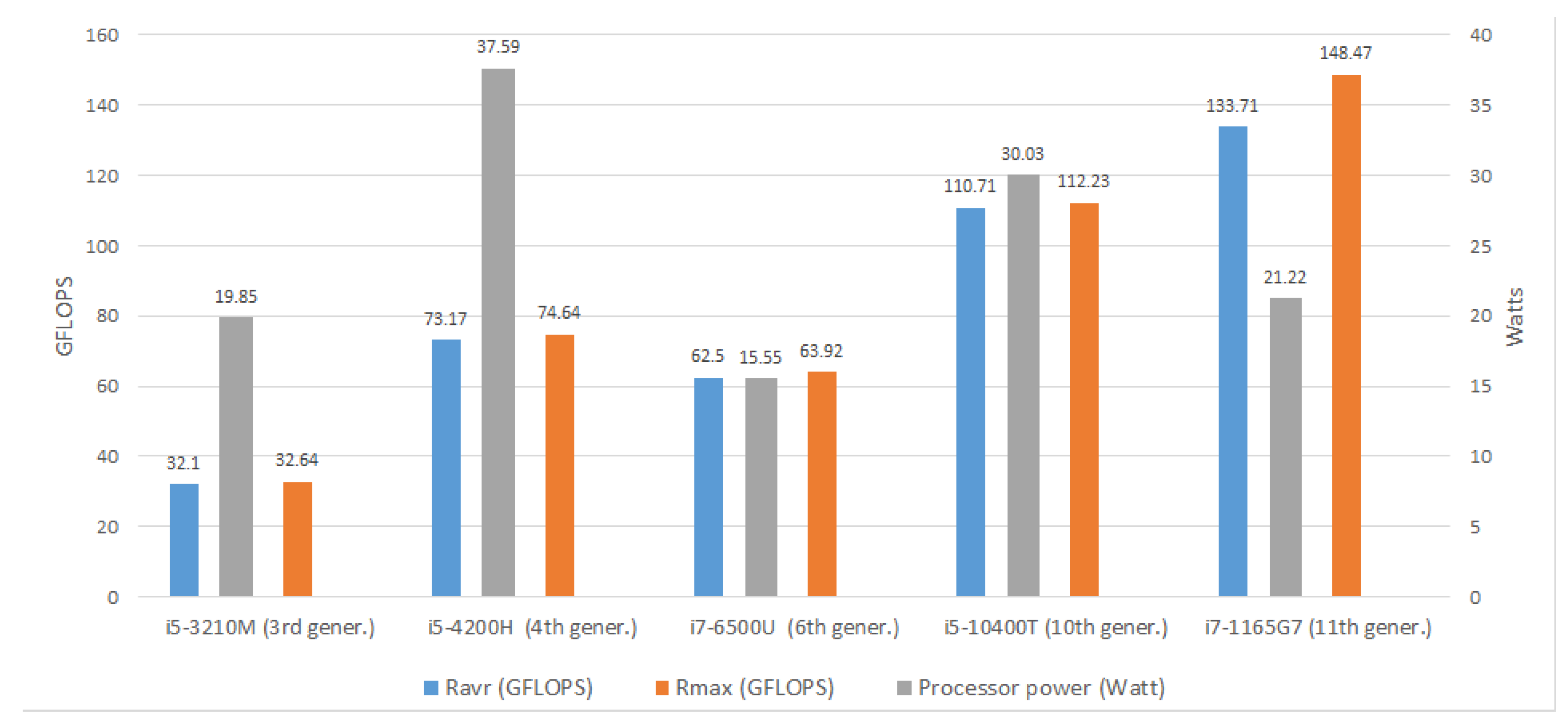
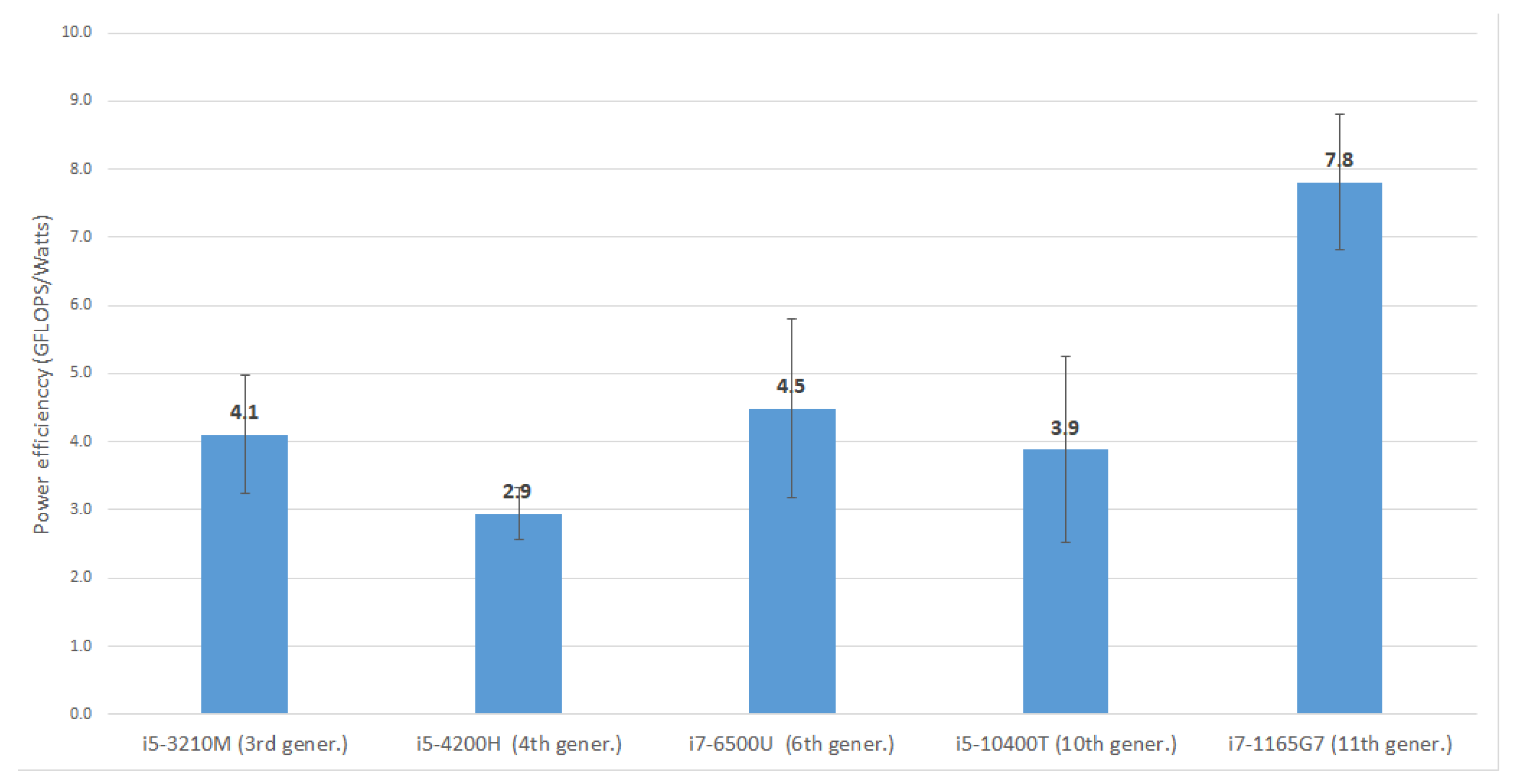
One data source available from Intel Power Gadget is the power of the processor (CPU) (see Table 6), which can be combined with the performance ratios of execution (Ravr and Rmax) obtained with Linpack. This is shown in Figure 14. It is also possible to obtain the energy efficiency of the specific domain of the isolated processors (UC + ALU + FPU + GT + other circuits on the microprocessor chip), as detailed in Table 12 and represented in Figure 15, where bars are included to depict the variability of the results. It is recalled that the standard deviation is a measure of the amount of variation or dispersion of a set of values and, in the present case, these deviations correspond to the fact that not all the machine instructions of a processor consume the same energy, and to the out-of-order execution, cache hits, and other run-time optimizations. These tests have been executed in multitask OS (Windows), so the CPU have to spend some time in another small processes, internal Kernel activities or attending network packets, so that during the execution of a program the values can spread over a wide range around the mean. In Figure 7, Figure 8, Figure 9, Figure 10, Figure 11, it is possible to observe both the power variations in the successive core phases and in the idle phases (baseline), which determine the value of the standard deviation. Even from Figure 11, it can be seen how the first run of Linpack contains at the beginning instructions different from the other four, probably to initialize the parameters and data of the program. All these variations are mathematically represented by the standard deviation, being greater as the fluctuations between the energy consumed by the instructions increase.
As a curiosity, Table 13 compares the energy efficiency of the Green500 supercomputers with the small systems analyzed. Information on the position of each platform in the Green500 and Top500 is included, and the maximum computing performance rate, average power, and power efficiency are also shown. Measures have been obtained in all cases with Linpack benchmark. Rows corresponding to the positions that the equipment under test would occupy within the classification have been added to the table.
As can be seen, the equipment under test obtains a higher power efficiency than some of the TOP500 supercomputers. It is important to note that in all cases the performance rate of the supercomputers is much higher than that of the systems under test. Thus, for example, although the SUT5 is more energy efficient than the JOLIOT-CURIE SKL (4.44 vs. 4.43 GFLOPS/W), a program that would take t = 1 second to be run on the supercomputer, would take exactly:
The energy consumed in the execution of NI float-point instructions can be easily obtained on a computer with power efficiency, PE. Indeed, by definition, power efficiency is:
Considering that the energy consumed, E, is the product of the average power, P, and the time elapsed in the execution of the program, t, it has:
That is, the total energy consumed during the execution of NI instructions is lower if the power efficiency is lower, regardless of the execution time of those NI instructions.
5. Conclusions and Future Work
In this work, the possibility of using PCs as a plausible, energy efficient option for the execution of non-complex scientific or engineering computer programs has been explored. For this purpose, five personal computers with different processors of different generations have been used, and measurements of performance rates of execution, electric power consumed, and power efficiency of the five systems under test have been calculated.
To demonstrate the plausibility of the proposed thesis, the results obtained have been compared with the rank and details of the 500 most powerful computer systems in the world (TOP500), including their energy efficiencies (GREEN500). The test tools and method followed for the measures presented are analogous to those used in the indicated rankings.
To meet the stated objective, a complete methodology has been presented to determine the energy efficiency of complete computer systems. Specifically, the energy efficiency of a computer system has been determined by executing Linpack, a reference application considered to be among the most used in scientific and engineering systems. This has been done using the (a) external meter oZm and the (b) Intel Power Gadget, an internal power meter that considers the counters and hardware registers included in the processor.
The Linpack program has been used as a reference for the measurements. This program is considered a very suitable benchmark to measure the computing power of a device executing instructions with float-point data, which is the most computationally complex type of data, requiring fast processing times and is representative of scientific and engineering applications.
The fact that a system has a higher power efficiency than another means that it consumes less energy (Wh) running the same program, regardless of the execution time. Despite the complexity of supercomputers, in some cases, their energy efficiency is similar to, or higher than, that of PCs when executing the same programs, as occurs in the first 78 supercomputers in the Green500 (Table 13).
Although the objective of this paper is only to compare the energy efficiency of PCs with high-performance computers in scientific-technical applications, the results obtained can be analyzed and exploited in greater depth. In this way, as future work it is possible to isolate and analyze in detail the behavior of Processor Power, IA Power, GT Power, DRAM Power, and the set of other computer components. The consumption of this last set of components would be obtained by the difference between the oZm measurements and those provided by Intel Power Gadget, and would include the consumption associated with data transfer via buses external to the processor, I/O ports, peripherals, power supply, etc. On the other hand, although the precision obtained with 5 measurements is a priori sufficient to make the comparative analysis with the GREEN500 systems, a more exhaustive analysis with more than 5 runs should be carried out to obtain a more reliable mean values. The main pitfall here is that a program such as Linpack, running on laptops, entails a very long execution time.
It is concluded that the power efficiency of PCs for the same workload is comparable to that of more powerful computers, which means that, in many cases where execution time is not constrained, it may be appropriate to migrate program execution from servers or workstations to personal computers in order to contribute to reducing the overall energy consumption produced by ICTs.
It should be noted that, according to the predictive models on electricity use by ICTs developed by Andrae and Edler [6], consumption of these technologies will increase from 13% of global electricity use in the world in 2022 to 21% in 2030, and could reach more than half (51%) of the earth’s total demand in the worst-case scenario. It is therefore necessary to analyze different options, as in this paper, to reduce the contribution of ICTs to the environmental impact.
Author Contributions
Data curation, J.C.G.-L.; formal analysis, J.J.E. and A.F.D.; writing—original draft, B.P.; writing—review and editing, T.L. All authors have read and agreed to the published version of the manuscript.
Funding
This research was partially funded by the Spanish Ministry of Science, Innovation, and Universities (MICIU) together with the European Regional Development Fund (ERDF), through the project PGC2018-098813-B-C31. Clarification: the grant number is PGC2018-098813-B-C31 and the funder includes MICIU and ERDF.
Institutional Review Board Statement
Not applicable.
Informed Consent Statement
Not applicable.
Data Availability Statement
Not applicable.
Acknowledgments
The authors would like to thank Alberto Prieto, Francisco Illeras (both from the Department of Computer Architecture and Technology of the University of Granada, Spain), and Francisco Gil (from the University of Almeria, Spain) for their valuable collaboration in this work.
Conflicts of Interest
The authors declare no conflict of interest.
References
- European Commission, 2030 Climate & Energy Framework. Available online: https://ec.europa.eu/clima/eu-action/climate-strategies-targets/2030-climate-energy-framework_en (accessed on 30 January 2022).
- Roco, M. Nanoscale Science and Engineering at NSF; National Science Foundation: Arlington, TX, USA, 2015. Available online: http://www.nseresearch.org/2015/presentations/NNI_15-1209_Grantees_MRoco_20%20min%20web.pdf (accessed on 26 August 2022).
- Semiconductor Industry Association and the Semiconductor Research Corporation, Rebooting the IT Revolution: A Call to Action. 2015. Available online: https://www.semiconductors.org/wp-content/uploads/2018/06/RITR-WEB-version-FINAL.pdf (accessed on 13 January 2022).
- Zhirnov, V.; Cavin, R.; Gammaitoni, L. Minimum Energy of Computing, Fundamental Considerations. In ICT-Energy-Concepts Towards Zero-Power Information and Communication Technology; IntechOpen: London, UK, 2014. [Google Scholar]
- Burgess, A.; Brown, T. By 2040, There May Not Be Enough Power for All Our Computers. HENNIK RESEARCH, 17 August 2016. 2021. Available online: https://www.themanufacturer.com/articles/by-2040-there-may-not-be-enough-power-for-all-our-computers/ (accessed on 31 January 2022).
- Andrae, A.S.; Edler, T. On global electricity usage of communication technology: Trends to 2030. Challenges 2015, 6, 117–157. [Google Scholar] [CrossRef] [Green Version]
- Freitag, C.; Berners-Lee, M.; Widdicks, K.; Knowles, B.; Blair, G.; Friday, A. The climate impact of ICT: A review of estimates, trends and regulations. arXiv 2022, arXiv:2102.02622. [Google Scholar]
- Malmodin, J.; Lundén, D. The energy and carbon footprint of the global ICT and E&M sectors 2010–2015. Sustainability 2018, 10, 3027. [Google Scholar] [CrossRef] [Green Version]
- Federal Ministry for Economic Affairs. Development of ICT-Related Electricity Demand in Germany (Report in German). 2015. Available online: https://www.bmwk.de/Redaktion/EN/Pressemitteilungen/2015/20151210-gabriel-studie-strombedarf-ikt.html (accessed on 31 January 2022).
- Federal Ministry for Economic Affairs and Climate Action. Information and Communication Technologies Consume 15% Less Electricity Due to Improved Energy Efficiency. 2015. Available online: https://www.bmwi.de/Redaktion/EN/Pressemitteilungen/2015/20151210-gabriel-studie-strombedarf-ikt.html (accessed on 31 January 2022).
- Shehabi, A.; Smith, S.J.; Sartor, D.A.; Brown, R.E.; Herrlin, M.; Koomey, J.G.; Masanet, E.R.; Horner, N.; Azevedo, I.L.; Lintner, W. United States Data Center Energy Usage Report. Berkeley Lab. 2016. Available online: https://eta.lbl.gov/publications/united-states-data-center-energy (accessed on 31 January 2022).
- Urban, B.; Shmakova, V.; Lim, B.; Roth, K. Energy Consumption of Consumer Electronics in U.S. Report to the CEA; Fraunhofer USA Center for Sustainable Energy Systems: Boston, MA, USA, 2014; Available online: https://www.ourenergypolicy.org/wp-content/uploads/2014/06/electronics.pdf (accessed on 20 August 2022).
- Andrae, A.S. Comparison of several simplistic high-level approaches for estimating the global energy and electricity use of ICT networks and data centers. Int. J. Green Technol. 2019, 5, 51. [Google Scholar] [CrossRef] [Green Version]
- Manganelli, M.; Soldati, A.; Martirano, L.; Ramakrishna, S. Strategies for Improving the Sustainability of Data Centers via Energy Mix, Energy Conservation, and Circular Energy. Sustainability 2021, 13, 6114. [Google Scholar] [CrossRef]
- Hamdi, N.; Walid, C. A survey on energy aware VM consolidation strategies. Sustain. Comput. Inform. Syst. 2019, 23, 80–87. [Google Scholar] [CrossRef]
- Bordage, F. The Environmental Footprint of the Digital World, GreenIT 20. 2020. Available online: https://www.greenit.fr/wp-content/uploads/2019/11/GREENIT_EENM_etude_EN_accessible.pdf (accessed on 31 January 2022).
- Google Data Centers. Hamina, Finland. A White Surprise. Available online: https://www.google.com/about/datacenters/locations/hamina/ (accessed on 31 January 2022).
- Landré, D.; Nicod, J.-M.; Christophe, V. Optimal standalone data centre renewable power supply using an offline optimization approach. Sustain. Comput. Inform. Syst. 2022, 34, 100627. [Google Scholar]
- Kumar, K.; Lu, Y.H. Cloud computing for mobile users: Can offloading computation save energy? Computer 2010, 43, 51–56. [Google Scholar] [CrossRef]
- Liu, Q.; Luk, W. Heterogeneous systems for energy efficient scientific computing. In Proceedings of the International Symposium on Applied Reconfigurable Computing, Hong Kong, China, 19–23 March 2012; Springer: Berlin/Heidelberg, Germany, 2012; pp. 64–75. [Google Scholar]
- Islam, A.; Debnath, A.; Ghose, M.; Chakraborty, S. A survey on task offloading in multi-access edge computing. J. Syst. Archit. 2021, 118, 102225. [Google Scholar] [CrossRef]
- Zhao, M.; Yu, J.J.; Li, W.T.; Liu, D.; Yao, S.; Feng, W.; She, C.; Quek, T.Q. Energy-aware task offloading and resource allocation for time-sensitive services in mobile edge computing systems. IEEE Trans. Veh. Technol. 2021, 70, 10925–10940. [Google Scholar] [CrossRef]
- Maray, M.; Shuja, J. Computation offloading in mobile cloud computing and mobile edge computing: Survey, taxonomy, and open issues. Mob. Inf. Syst. 2022, 2022, 1121822. [Google Scholar] [CrossRef]
- Asadi, A.N.; Azgomi, M.A.; Entezari-Maleki, R. Analytical evaluation of resource allocation algorithms and process migration methods in virtualized systems. Sustain. Comput. Inform. Syst. 2020, 25, 100370. [Google Scholar] [CrossRef]
- ThermoFisher Scientific. StepOne Real-Time PCR System, Laptop. Available online: https://www.thermofisher.com/order/catalog/product/4376373 (accessed on 31 January 2022).
- BioTeke. Ultra-Fast Portable PCR Machine. Available online: https://www.bioteke.cn/4-channel-rapid-POC-Ultra-fast-portable-PCR-machine-pd04043964.html (accessed on 31 January 2022).
- Qureshi, B.; Alwehaibi, S.; Koubaa, A. On Power Consumption Profiles for Data Intensive Workloads in Virtualized Hadoop Clusters. In Proceedings of the 2017 IEEE Conference on Computer Communications Workshops (INFOCOM WKSHPS), Atlanta, GA, USA, 1–4 May 2017; pp. 42–47. [Google Scholar] [CrossRef] [Green Version]
- Mollova, S.; Simionov, R.; Seymenliyski, K. A study of the energy efficiency of a computer cluster. In Proceedings of the Seventh International Conference on Telecommunications and Remote Sensing, Barcelona, Spain, 8–9 October 2018; pp. 51–54. [Google Scholar]
- Qureshi, B.; Koubaa, A. On Energy Efficiency and Performance Evaluation of Single Board Computer Based Clusters: A Hadoop Case Study. Electronics 2019, 8, 182. [Google Scholar] [CrossRef] [Green Version]
- Warade, M.; Schneider, J.-G.; Lee, K. Measuring the Energy and Performance of Scientific Workflows on Low-Power Clusters. Electronics 2022, 11, 1801. [Google Scholar] [CrossRef]
- Xu, X.; Dou, W.; Zhang, X.; Chen, J. EnReal: An energy-aware resource allocation method for scientific workflow executions in cloud environment. IEEE Trans. Cloud Comput. 2015, 4, 166–179. [Google Scholar] [CrossRef]
- Khaleel, M.; Zhu, M.M. Energy-aware job management approaches for workflow in cloud. In Proceedings of the 2015 IEEE International Conference on Cluster Computing, Chicago, IL, USA, 8–11 September 2015; pp. 506–507. [Google Scholar]
- Mishra, S.K.; Puthal, D.; Sahoo, B.; Jayaraman, P.P.; Jun, S.; Zomaya, A.Y.; Ranjan, R. Energy-efficient VM-placement in cloud data center. Sustain. Comput. Inform. Syst. 2018, 20, 48–55. [Google Scholar] [CrossRef]
- Escobar, J.J.; Ortega, J.; Díaz, A.F.; González, J.; Damas, M. Time-energy Analysis of Multi-level Parallelism in Heterogeneous Clusters: The Case of EEG Classification in BCI Tasks. J. Supercomput. 2019, 75, 3397–3425. [Google Scholar] [CrossRef]
- Qureshi, B. Profile-based power-aware workflow scheduling framework for energy-efficient data centers. Future Gener. Comput. Syst. 2019, 94, 453–467. [Google Scholar] [CrossRef]
- Ji, K.; Zhang, F.; Chi, C.; Song, P.; Zhou, B.; Marahatta, A.; Liu, Z. A Joint Energy Efficiency Optimization Scheme Based on Marginal Cost and Workload Prediction in Data Centers. Sustain. Comput. Inform. Syst. 2021, 32, 100596. [Google Scholar] [CrossRef]
- Feng, W.C.; Cameron, K. The green500 list: Encouraging sustainable supercomputing. Computer 2007, 40, 50–55. [Google Scholar] [CrossRef]
- Top500, The Linpack Benchmark. Available online: https://www.top500.org/project/linpack/ (accessed on 31 January 2022).
- Linpack Xtreme. TechPowerUp, 31 December 2020 Version. Available online: https://www.techpowerup.com/download/linpack-xtreme/ (accessed on 31 January 2022).
- Viciana, E.; Alcayde, A.; Montoya, F.G.; Baños, R.; Arrabal-Campos, F.M.; Zapata-Sierra, A.; Manzano-Agugliaro, F. OpenZmeter: An efficient low-cost energy smart meter and power quality analyzer. Sustainability 2018, 10, 4038. [Google Scholar] [CrossRef]
- Hernandez, W.; Calderón-Córdova, C.; Brito, E.; Campoverde, E.; González-Posada, V.; Zato, J.G. A method of verifying the statistical performance of electronic circuits designed to analyze the power quality. Measurement 2016, 93, 21–28. [Google Scholar] [CrossRef]
- What Is openZmeter? Available online: https://openzmeter.com/ (accessed on 31 January 2022).
- Weaver, V.M.; Johnson, M.; Kasichayanula, K.; Ralph, J.; Luszczek, P.; Terpstra, D.; Moore, S. Measuring energy and power with PAPI. In Proceedings of the 2012 41st International Conference on Parallel Processing Workshops, Pittsburgh, PA, USA, 10–13 September 2012. [Google Scholar] [CrossRef] [Green Version]
- Intel® 64 and IA-32 Architectures Software Developer’s Manual Manual Volume 3. pp. 14–31 to 14–39. Available online: https://www.intel.com/content/www/us/en/architecture-and-technology/64-ia-32-architectures-software-developer-system-programming-manual-325384.html (accessed on 31 January 2022).
- Khan, K.N.; Hirki, M.; Niemi, T.; Nurminen, J.K.; Ou, Z. RAPL in action: Experiences in using RAPL for power measurements. ACM Trans. Modeling Perform. Eval. Comput. Syst. 2018, 3, 9. [Google Scholar] [CrossRef]
- Intel Processors for All That You Do. Available online: https://www.intel.com/content/www/us/en/products/details/processors.html (accessed on 31 January 2022).
- Meuer, H.; Strohmaier, E.; Dongarra, J.; Simon, H. The Top500 Project. 2010. Available online: https://top500.org/files/TOP500_MS-Industriekunden_16_10_2008.pdf (accessed on 31 January 2022).
- TOP500. The List. Available online: https://www.top500.org/lists/green500/ (accessed on 31 January 2022).
- EEHPC. Energy Efficient High Performance Computing Power Measurement Methodology (version 2.0 RC 1.0). Energy Efficient High Performance Computing Working Group (EEHPC WG). Available online: https://www.top500.org/static/media/uploads/methodology-2.0rc1.pdf (accessed on 26 August 2022).
- IRDS. International Roadmap for Devices and Systems 2022 Edition Executive Summary. 2022, p. 27. Available online: https://irds.ieee.org/images/files/pdf/2022/2022IRDS_ES.pdf (accessed on 26 August 2022).
- Green500 List June 2022. Available online: https://www.top500.org/lists/green500/list/2022/06/ (accessed on 26 August 2022).
Figure 1.
Andrae and Edler’s projections for ICT electrical energy use (TWh) by year.

Figure 2.
Screenshot of a Linpack Xtreme benchmark run: parameters used and the results of the run.

Figure 3.
Simplified scheme of the oZm.

Figure 4.
Dashboard of oZm. From top to bottom and left to right: active energy, RMS voltage, RMS current, active power and frequency.
Figure 4.
Dashboard of oZm. From top to bottom and left to right: active energy, RMS voltage, RMS current, active power and frequency.

Figure 5.
Power domains considered in RAPL interface.

Figure 6.
Intel Power Gadget tool: (a) input options and (b) graphic results.

Figure 7.
SUT1 power (Watts) versus time (h:m:s): (a) Power Gadget power measures and (b) oZm power measures.
Figure 7.
SUT1 power (Watts) versus time (h:m:s): (a) Power Gadget power measures and (b) oZm power measures.

Figure 8.
SUT2 power (Watts) versus time (h:m:s): (a) Power Gadget power measures and (b) oZm power measures.
Figure 8.
SUT2 power (Watts) versus time (h:m:s): (a) Power Gadget power measures and (b) oZm power measures.

Figure 9.
SUT3 power (Watts) versus time (h:m:s): (a) Power Gadget power measures and (b) oZm power measures.
Figure 9.
SUT3 power (Watts) versus time (h:m:s): (a) Power Gadget power measures and (b) oZm power measures.

Figure 10.
SUT4 power (Watts) versus time (h:m:s): (a) Power Gadget power measures and (b) oZm power measures.
Figure 10.
SUT4 power (Watts) versus time (h:m:s): (a) Power Gadget power measures and (b) oZm power measures.

Figure 11.
SUT5 power (Watts) versus time (h:m:s) (a) Power Gadget power measures and (b) oZm power measures.
Figure 11.
SUT5 power (Watts) versus time (h:m:s) (a) Power Gadget power measures and (b) oZm power measures.

Figure 12.
Performance rates and power consumed during the run of Linpack in the five SUTs.

Figure 13.
Energy consumed and power efficiency during the run of Linpack in the five SUTs.

Figure 14.
Performance rates of execution and average power consumed during the run of Linpack in the five microprocessors.
Figure 14.
Performance rates of execution and average power consumed during the run of Linpack in the five microprocessors.

Figure 15.
Power efficiency of the microprocessors measured during the Linpack run.


Table 1.
Parameters used in Linpack Xtreme.
| Parameters to be Set: |
|---|
| Number of equations to solve |
| Leading array dimension |
| Number of times to run Linpack (which can be performed from 1 to 5 times, successively) |
| Data space alignment value (in Kbytes) |
| Maximum memory to be used |
| Generated Results: |
| CPU frequency (GHz) |
| Number of CPUs |
| Number of cores |
| Number of threads |
| Size |
| LDA (leading array dimension) |
| Data alignment value (Kbytes) |
| Time (s) |
| Residual |
| Residual (norm) |
| Raverage (GFlops) |
| Rmaximal (GFlops), Maximal Linpack performance achieved |
Table 2.
Sample of the parameters measured by oZm corresponding to a fragment made with one of the tested systems during the execution of Linpack (Section 4).
Table 2.
Sample of the parameters measured by oZm corresponding to a fragment made with one of the tested systems during the execution of Linpack (Section 4).
| Time | Active Power | Reactive Power | Power Factor | Phi | Voltage THD | Current THD |
|---|---|---|---|---|---|---|
| 6:53 | 36.768 | –7.407 | 0.448 | 23.068 | 3.61 | 296.687 |
| 6:54 | 27.966 | –5.26 | 0.501 | 10.54 | 3.53 | 344.986 |
| 6:55 | 21.681 | –4.636 | 0.478 | 12.179 | 3.552 | 364.808 |
| 6:56 | 20.624 | –4.542 | 0.474 | 12.676 | 3.579 | 368.612 |
| 6:57 | 19.029 | –4.366 | 0.466 | 13.081 | 3.533 | 377.501 |
| 6:58 | 19.432 | –4.36 | 0.465 | 12.831 | 3.595 | 383.131 |
| 6:59 | 19.214 | –4.136 | 0.462 | 12.33 | 3.676 | 388.315 |
| 7:00 | 18.982 | –4.301 | 0.464 | 12.857 | 3.647 | 384.47 |
| 7:01 | 19.07 | –4.414 | 0.464 | 13.232 | 3.638 | 383.253 |
| 7:02 | 18.992 | –4.368 | 0.466 | 13.126 | 3.673 | 381.309 |
| 7:03 | 19.835 | –4.492 | 0.469 | 12.929 | 3.615 | 376.45 |
| 7:04 | 20.227 | –4.477 | 0.466 | 12.666 | 3.679 | 383.472 |
| 7:05 | 16.921 | –4.239 | 0.449 | 14.662 | 3.642 | 399.679 |
| 7:06 | 16.903 | –4.204 | 0.454 | 14.285 | 3.682 | 394.078 |
| 7:07 | 16.252 | –4.207 | 0.449 | 14.95 | 3.686 | 394.636 |
| 7:08 | 16.644 | –4.348 | 0.454 | 15.116 | 3.609 | 384.211 |
THD: measure of the Total Harmonic Distortion present in the voltage or current signals.
Table 3.
Sample data provided by Intel Power Gadget for the first 10 s.
| System Time | RDTSC | Elapsed Time (sec) | CPU Utilization (%) | CPU Frequency_0 (MHz) | Processor Power_0 (W) | Cumulative Processor Energy_0 (J) | Cumulative Processor Energy_0 (mWh) |
|---|---|---|---|---|---|---|---|
| 11:44:17:227 | 3.04 × 10¹² | 0.988 | 28 | 2900 | 11.976 | 11.829 | 3.286 |
| 11:44:18:247 | 3.04 × 10¹² | 2.008 | 16 | 1200 | 7.69 | 19.674 | 5.465 |
| 11:44:19:254 | 3.04 × 10¹² | 3.015 | 21 | 2900 | 9.021 | 28.759 | 7.989 |
| 11:44:20:247 | 3.05 × 10¹² | 4.009 | 26 | 2900 | 11.621 | 40.307 | 11.196 |
| 11:44:21:246 | 3.05 × 10¹² | 5.007 | 41 | 2900 | 13.08 | 53.371 | 14.825 |
| Etc. | |||||||
| IA Power_0 (W) | Cumulative IA Energy_0 (J) | Cumulative IA Energy_0 (mWh) | Package Temperature_0 (C) | Package Hot_0 | GT Power_0 (W) | Cumulative GT Energy_0 (J) | Cumulative GT Energy_0 (mWh) |
| 9.514 | 9.398 | 2.61 | 69 | 0 | 0.024 | 0.024 | 0.007 |
| 5.282 | 14.785 | 4.107 | 59 | 0 | 0.04 | 0.064 | 0.018 |
| 6.646 | 21.478 | 5.966 | 66 | 0 | 0.017 | 0.081 | 0.023 |
| 9.226 | 30.646 | 8.513 | 71 | 0 | 0.012 | 0.093 | 0.026 |
| 10.528 | 41.161 | 11.434 | 69 | 0 | 0.023 | 0.116 | 0.032 |
| Etc. | |||||||
| Package PL1_0 (W). | Package PL2_0 (W) | Package L4_0(W) | Platform PsysPL1_0 (W) | Platform PsysPL2_0(W) | GT Frequency (MHz) | GT Utilization (%) | |
| 35 | 44 | 112 | 0 | 0 | 99,999,999 | 0 | |
| 35 | 44 | 112 | 0 | 0 | 99,999,999 | 0 | |
| 35 | 44 | 112 | 0 | 0 | 99,999,999 | 0 | |
| 35 | 44 | 112 | 0 | 0 | 99,999,999 | 0 | |
| 35 | 44 | 112 | 0 | 0 | 99,999,999 | 0 | |
| Etc. |
Table 4.
Parameters supplied by Intel Power Gadget.
| Parameter | Observation |
|---|---|
| System Time | Current time (hh:mm:ss). |
| RDTSC | Time Stamp Counter (TSC), number of CPU cycles since its reset. |
| Elapsed Time | In seconds. |
| CPU Utilization | Central processor unit usage percentage (%). |
| CPU Frequency_0 | CPU frequency (MHz). |
| Processor Power_0 | Power consumed by UC + ALU + FPU + integrated graphics + others (W). |
| IA Power_0 | Power consumed by UC + ALU + FPU (W). |
| Package Temperature_0 | Chip temperature (°C). |
| DRAM Power_0 | Power consumed by DRAM attached to the integrated memory controller (W). |
| GT Power_0 | Power consumed by the discrete graphic processor (W). |
| Package PL1_0 | Limit (threshold) for average package1; power that will not be exceeded (W). |
| Package PL2_0 | Limit (threshold) for average package2; power that will not be exceeded (W). |
| Package PL4_0 | Limit (threshold) for average package4; power that will not be exceeded (W). |
| Platform PsysPL1_0 | Limit (threshold) for average platform1; power that will not be exceeded. The platform is the entire socket (W). |
| Platform PsysPL2_0 | Limit (threshold) for average platform2; power that will not be exceeded (W). |
| GT Frequency | Frequency of the integrated graphic processor unit (GPU) (MHz). |
| GT Utilization (%) | Usage percentage of the integrated graphic processor unit (GPU) (%). |
Table 5.
Systems under test.
| SUT1 | SUT2 | SUT3 | SUT4 | SUT5 | |
|---|---|---|---|---|---|
| Reference: | Sony Vaio SVZ1311C5E | ASUS Notebook X550J | Toshiba Portege Z30-C | HP Pavilion All-in-One K1987LF | ASUS Expertbook B9400CEA |
| Processor: | Core i5-3210M 2.5 GHz | Core i5-4200H 2.8 GHz | Core i7-6500U 2.5 GHz | Core i5-10400T 2 GHz | Core i7-1165G7 2.8 GHz |
| Kernels: | 2 cores, 4 threads | 2 cores, 4 threads | 2 cores, 4 threads | 6 cores, 12 threads | 4 cores, 8 threads |
| Memory capacity: | 8 GB | 8 GB | 16 GB | 16 GB | 16 GB |
| Hard disk: | SSD 256 GB | HDD 500 GB | SSD 1 TB | SSD 512 GB | SSD 1 TB |
| Mainboard: | SONY VAIO | ASUS X550J | TOSHIBA | HP 86ED | ASUS Tek |
| Graphics card: | Intel HD Graphics 4000 | NVIDIA GeForce GTX 850M | Intel HD Graphics 520 | UHD Graphics 630 | Intel Iris Xe |
| AC/DC adapter: | Out: 19.5V-33mA. In: 100-240V-1.5A | Out: 19V-6.32 A In: 100-240V-6.32 A | Out: 19.5V-2.37A. In: 100-240V-1.2A | Out: 19.5 V-7.7 A In: 100-240 V-2.5 A | Out: 5-15V 3A. In: 100-240V-1.5A |
| Operating system: | Windows 10 Home | Windows 10 Pro | Windows 10 home | Windows 10 Home | Windows 10 Pro |
| Other Processor Features: | |||||
| Generation: | 3rd | 4th | 6th | 10th | 11th |
| Lithography: | 22 nm | 22 nm | 14 nm | 14 nm | 10 nm |
| Frequency: | 2.5–3.10 GHz | 2.8–3.4 GHz | 2.5–3.10 GHz | 2–3.6 GHz | 4.7 GHz |
| Cache size: | 3 MB | 3 MB | 4 MB | 12 MB | 12 MB |
| Max. memory size: | 32 GB | 32 GB | 32 GB | 128 GB | 64 GB |
| Processor launch date: | Q2, 2012 | Q4, 2013 | Q3, 2015 | Q2, 2020 | Q3, 2020 |
| TDP: | 35 W | 47 W | 15 W | 25 W | 12 W |
| TJuntion: | 105 °C | 100 °C | 100 °C | 100 °C | 100 °C |
Table 6.
Summary of the main results obtained in the five systems under test.
| Systems under Test → | SUT1 | SUT2 | SUT3 | SUT4 | SUT5 |
|---|---|---|---|---|---|
| Linpack Extreme Results: | |||||
| Number of CPUs | 1 | 1 | 1 | 1 | 1 |
| Number of cores | 2 | 2 | 2 | 6 | 4 |
| Number of threads used | 2 | 2 | 2 | 6 | 4 |
| Number of trials to run | 5 | 5 | 5 | 5 | 5 |
| Number of equations to solve | 20,000 | 20,000 | 20,000 | 20,000 | 20,000 |
| Data alignment value (KB) | 4 | 4 | 4 | 4 | 4 |
| Time of a trial | 164.29 ± 4.42 | 72.9 ± 1.58 | 85.45 ± 3.40 | 48.19 ± 0.80 | 40.01 ± 2.29 |
| R average (GFlops) | 32.1 ± 0.83 | 73.17 ± 1.56 | 62.50 ± 2.36 | 110.71 ± 1.80 | 133.71 ± 8.27 |
| R maximal (GFlops) | 32.64 | 74.64 | 63.92 | 112.23 | 148.47 |
| Intel Power Gadget Results: | |||||
| RDTSC (number of cycles) | 1.22 × 10¹² | 1.94 × 10¹¹ | 2.19 × 10¹¹ | 9.20 × 10¹⁰ | 1.12 × 10¹¹ |
| Elapsed Time (s) | 158.01 ± 19.05 | 69.61 ± 2.58 | 84.4 ± 3.3 | 46.17 ± 0.7 | 39.90 ± 2.17 |
| CPU Frequency (GHz) | 2.882 | 3.390 | 2.486 | 3.281 | 4.606 |
| CPU Utilization (%) | 75.15 ± 1.64 | 69.61 ± 2.58 | 57.54 ± 3.08 | 51.12 ± 1.04 | 51.45 ± 0.51 |
| Processor Power (W) | 19.85 ± 0.06 | 37.59 ± 0.25 | 15.55 ± 0.17 | 30.03 ± 0.06 | 21.22 ± 1.94 |
| IA Power (W) | 16.99 ± 0.05 | 27.68 ± 0.35 | 10.31 ± 3.29 | 29.19 ± 0.06 | 16.84 ± 2.02 |
| GT Power (W) | 0.0203 ± 0.0003 | 2.33 ± 0.09 | 0.007 ± 0.002 | 2.33 ± 0.09 | 0.0118 ± 0.0004 |
| DRAM Power (W) | - | 3.353 ± 0.005 | 2.66 ± 0.40 | 2.825 ± 0.007 | 0 |
| Package Temperature (°C) | 82.94 ± 0.49 | 96.13 ± 0.88 | 70.75 ± 6.08 | 64.39 ± 2.45 | 82.05 ± 1.05 |
| oZm Results: | |||||
| Active power (Pavrg) (W) | 45.94 ± 1.12 | 35.95 ± 1.06 | 93.42 ± 0.80 | 68.72 ± 1.54 | 33.42 ± 2.41 |
| Time of trial run (s) | 166.28 ± 4.20 | 85.45 ± 3.40 | 72.92 ± 1.58 | 48.19 ± 0.80 | 39.9 ± 2.17 |
Table 7.
SUT1 results in the core and idle (baseline) phases.
| SUT1 (Sony Vaio) | Total in Core Phase | Baseline Phases | Attributable to Linpack Execution | |
|---|---|---|---|---|
| Intel Power Gadget measures | CPU Utilization (%) | 75.15 ± 1.64 | 29.69 ± 12.42 | 45.46 |
| Processor Power (Watt) | 19.85 ± 0.06 | 11.90 ± 2.52 | 7.95 | |
| IA Power (Watt) | 16.99 ± 0.05 | 12.52 ± 0.45 | 4.47 | |
| GT Power (Watt) | 0.0203 ± 0.0003 | 0.017 ± 0.002 | 0.0033 | |
| DRAM Power (Watt) | - | - | ||
| Package Temperature (°C) | 82.94 ± 0.49 | 73.41 ± 0.98 | 9.53 | |
| openZmeter | Active power | 45.94 ± 1.12 | 30.37 ± 4.98 | 15.57 |
Table 8.
SUT2 results in the core and idle (baseline) phases.
| SUT 2 (ASUS Notebook) | Total in Core Phase | Baseline Phases | Attributable to Linpack Execution | |
|---|---|---|---|---|
| Intel Power Gadget measures | CPU Utilization (%) | 69.61 ± 2.58 | 15.63 ± 1.61 | 53.98 |
| Processor Power (Watt) | 37.59 ± 0.25 | 12.19 ± 1.56 | 25.40 | |
| IA Power (Watt) | 27.68 ± 0.35 | 15.05 ± 3.82 | 12.63 | |
| GT Power (Watt) | 2.33 ± 0.09 | 2.7 ± 0.31 | –0.37 | |
| DRAM Power (Watt) | 3.353 ± 0.005 | 1.88 ± 0.10 | 1.473 | |
| Package Temperature (°C) | 96.13 ± 0.88 | 85.37 ± 5.73 | 10.76 | |
| openZmeter | Active Power | 93.42 ± 0.80 | 58.53 ± 12.08 | 34.89 |
Table 9.
SUT3 results in the core and idle (baseline) phases.
| SUT3 (Toshiba Portege) | Total in Core Phase | Baseline Phases | Attributable to Linpack Execution | |
|---|---|---|---|---|
| Intel Power Gadget measures | CPU Utilization (%) | 57.54 ± 3.08 | 15.63 ± 1.61 | 53.98 |
| Processor Power (Watt) | 15.55 ± 0.17 | 1.30 ± 0.38 | 14.25 | |
| IA Power (Watt) | 10.31 ± 3.29 | 5.66 ± 2.23 | 4.65 | |
| GT Power (Watt) | 0.01 ± 0.00 | 0.01 ± 0.00 | 0 | |
| DRAM Power (Watt) | 2.66 ± 0.40 | 1.70 ± 0.10 | 0.96 | |
| Package Temperature (°C) | 70.75 ± 6.08 | 62.59 ± 9.59 | 8.16 | |
| openZmeter | Active Power | 35.95 ± 1.06 | 18.37 ± 3.98 | 17.58 |
Table 10.
SUT4 results in the core and idle (baseline) phases.
| SUT 4 (HP Pavilion) | Total in Core Phase | Baseline Phases | Attributable to Linpack Execution | |
|---|---|---|---|---|
| Intel Power Gadget measures | CPU Utilization (%) | 51.12 ± 1.04 | 0.85 ± 0.26 | 50.27 |
| Processor Power (Watt) | 30.03 ± 0.06 | 1.14 ± 0.40 | 28.89 | |
| IA Power (Watt) | 29.19 ± 0.06 | 14.69 ± 3.74 | 14.5 | |
| GT Power (Watt) | 2.33 ± 0.09 | 2.70 ± 0.31 | –0.37 | |
| DRAM Power (Watt) | 2.825 ± 0.007 | 0.89 ± 0.07 | 1.94 | |
| Package Temperature (°C) | 64.39 ± 2.45 | 57.53 ± 5.72 | 6.86 | |
| openZmeter | Active Power | 68.72 ± 1.54 | 30.74 ± 6.06 | 37.98 |
Table 11.
SUT5 results in the core and idle (baseline) phases.
| SUT5 (ASUS Experbook) | Total in Core Phase | Baseline Phases | Attributable to Linpack Execution | |
|---|---|---|---|---|
| Intel Power Gadget measures | CPU Utilization (%) | 51.45 ± 0.51 | 2.54 ± 1.73 | 48.91 |
| Processor Power (Watt) | 21.22 ± 1.94 | 2.31 ± 0.25 | 18.70 | |
| IA Power (Watt) | 16.84 ± 2.02 | 1.03 ± 0.95 | 15.81 | |
| GT Power (Watt) | 0.0118 ± 0.0004 | 0.025 ± 0.007 | –0.02 | |
| DRAM Power (Watt) | - | - | - | |
| Package Temperature (°C) | 82.05 ± 1.05 | 47.06 ± 4.51 | 34.99 | |
| openZmeter | Active Power | 33.42 ± 2.41 | 11.79 ± 3.81 | 21.63 |
Table 12.
Energy efficiency of the microprocessors in the execution of Linpack measured with the Power Gadget.
Table 12.
Energy efficiency of the microprocessors in the execution of Linpack measured with the Power Gadget.
| Processor Power (Watt) | Baseline Phases (Watt) | Atributable to Linpack Execution (Watt) | Rmax (GFLOPS) | Power Efficiency (GFLOPS/Watt) | RSD (Relative Standard Deviation) | |
|---|---|---|---|---|---|---|
| i5-3210M (3rd gener.) | 19.85 ± 0.06 | 11.90 ± 2.52 | 7.95 ± 1.69 | 32.64 | 4.1 ± 0.87 | 0.21 |
| i5-4200H (4th gener.) | 37.59 ± 0.25 | 12.19 ± 1.56 | 25.40 ± 3.27 | 74.64 | 2.9 ± 0.38 | 0.13 |
| i7-6500U (6th gener.) | 15.55 ± 0.17 | 1.30 ± 0.38 | 14.25 ± 4.18 | 63.92 | 4.5 ± 1.32 | 0.29 |
| i5-10400T (10th gener.) | 30.03 ± 0.06 | 1.14 ± 0.40 | 28.89 ± 10.14 | 112.28 | 3.9 ± 1.36 | 0.36 |
| i7-1165G7 (11th gener.) | 21.22 ± 1.94 | 2.31 ± 0.25 | 19.01 ± 2.40 | 148.47 | 7.8 ± 0.99 | 0.13 |
Table 13.
Position in terms of power efficiency of the systems under test within the Green500 list (June 2022) [51].
Table 13.
Position in terms of power efficiency of the systems under test within the Green500 list (June 2022) [51].
| Platform | Position in Green500 | Position in TOP500 | Rmax TFLOP/s | Power (KW) | Power Efficiency (GFLOPS/Watt) |
|---|---|---|---|---|---|
| Frontier TDS-HPE Cray EX235a, AMD Oak Ridge National Laboratory United States | 1 | 29 | 19,200 | 309 | 62.684 |
| Frontier-HPE Cray EX235a, AMD Oak Ridge National Laboratory United States | 2 | 1 | 1,102,000 | 21 | 52.227 |
| * SUT5. ASUS 2 | – | – | 0.148 | 0.03347 | 4.436 |
| JOLIOT-CURIE SKL-CEA/TGCC-GENCI, FRANCE | 92 | 124 | 4070 | 917 | 4.434 |
| * SUT2. Toshiba 1 | – | – | 0.064 | 0.0359 | 1.779 |
| occigen2. National de Calcul Intensif-Centre Informatique National de l’Enseignement Suprieur (GENCI-CINES) FRANCE | 167 | 255 | 2490 | 1430 | 1.745 |
| * SUT4. HP | – | – | 0.112 | 0.06872 | 1.633 |
| HKVDPSystem, IT Service Provider, CHINA | 172 | 388 | 1980 | 1216 | 1.627 |
| * SUT3. ASUS | – | – | 0.075 | 0.09342 | 0.7989 |
| * SUT1. SONY | – | – | 0.037 | 0.04594 | 0.7923 |
| Thunder-SGI ICE X, Xeon E5-2699v3/E5-2697 v3, Infiniband FDR, NVIDIA Tesla K40, Intel Xeon Phi 7120P, HPE, Air Force Research Laboratory, United States | 183 | 171 | 3130 | 4820 | 0.649 |
* System under test.
Publisher’s Note: MDPI stays neutral with regard to jurisdictional claims in published maps and institutional affiliations. |
© 2022 by the authors. Licensee MDPI, Basel, Switzerland. This article is an open access article distributed under the terms and conditions of the Creative Commons Attribution (CC BY) license (https://creativecommons.org/licenses/by/4.0/).
Share and Cite
MDPI and ACS Style
Prieto, B.; Escobar, J.J.; Gómez-López, J.C.; Díaz, A.F.; Lampert, T. Energy Efficiency of Personal Computers: A Comparative Analysis. Sustainability 2022, 14, 12829. https://doi.org/10.3390/su141912829
AMA Style
Prieto B, Escobar JJ, Gómez-López JC, Díaz AF, Lampert T. Energy Efficiency of Personal Computers: A Comparative Analysis. Sustainability. 2022; 14(19):12829. https://doi.org/10.3390/su141912829
Chicago/Turabian StylePrieto, Beatriz, Juan José Escobar, Juan Carlos Gómez-López, Antonio F. Díaz, and Thomas Lampert. 2022. "Energy Efficiency of Personal Computers: A Comparative Analysis" Sustainability 14, no. 19: 12829. https://doi.org/10.3390/su141912829
Note that from the first issue of 2016, this journal uses article numbers instead of page numbers. See further details here.