Article

A Biogeography-Based Optimization with a Greedy Randomized Adaptive Search Procedure and the 2-Opt Algorithm for the Traveling Salesman Problem

1
Department of Electronic Engineering, National Kaohsiung University of Science and Technology, Kaohsiung 80778, Taiwan
2
Department of Computer Science and Information Engineering, National Penghu University of Science and Technology, Magong 88046, Taiwan
3
Department of Business Administration, Tainan University of Technology, Tainan 71002, Taiwan
4
Ph.D. Program in Biomedical Engineering, Kaohsiung Medical University, Kaohsiung 80708, Taiwan
5
School of Dentistry, Kaohsiung Medical University, Kaohsiung 80708, Taiwan
6
Drug Development and Value Creation Research Center, Kaohsiung Medical University, Kaohsiung 80708, Taiwan
7
Department of Political Science, National Cheng Kung University, Tainan 701401, Taiwan
*
Authors to whom correspondence should be addressed.
Sustainability 2023, 15(6), 5111; https://doi.org/10.3390/su15065111
Submission received: 24 December 2022 / Revised: 1 February 2023 / Accepted: 9 February 2023 / Published: 14 March 2023
(This article belongs to the Special Issue Application of Green Energy Technology in Sustainable Environment)

Abstract

:
We develop a novel method to improve biogeography-based optimization (BBO) for solving the traveling salesman problem (TSP). The improved method is comprised of a greedy randomized adaptive search procedure, the 2-opt algorithm, and G2BBO. The G2BBO formulation is derived and the process flowchart is shown in this article. For solving TSP, G2BBO effectively avoids the local minimum problem and accelerates convergence by optimizing the initial values. To demonstrate, we adopt three public datasets (eil51, eil76, and kroa100) from TSPLIB and compare them with various well-known algorithms. The results of G2BBO as well as the other algorithms perform close enough to the optimal solutions in eil51 and eil76 where simple TSP coordinates are considered. In the case of kroa100, with more complicated coordinates, G2BBO shows greater performance over other methods.

1. Introduction

Optimizing a pragmatic method to solve the traveling salesman problem (TSP) [1] provides immediate applications [2,3] in the real world. For example, the highly complex applied logistics planning industry can reduce operating expenses because the energy expended to calculate the routes are dwarfed by the energy used for transport services such as air mail/cargo, marine container shipping, train cargo and end-mile package delivery.
The approaches for solving TSP generally fall under two general types: (1) searching for the optimal traversal solution [4] and (2) searching for an approximate solution [5,6] with shorter calculation time compared to the optimal solution.
Most existing research chooses the second approach and provides a method to find an approximate solution in an acceptable time. Although the resulting solution is only near the optimal solution, it is provided much faster than the time and computationally heavy exhaustive search for the optimal solution. Therefore, finding an efficient approximation to replace the exhaustive search for the optimal solution is the current direction of research.
BBO is a meta-heuristic optimization algorithm inspired by species biogeography [7,8]. It solves optimization problems in various fields, including machine learning, engineering, and operational research. The basic idea behind BBO is to explore the search space for optimization problems using biogeography principles such as migration and speciation.
BBO’s advantages are that it can address problems with multiple objectives and constraints, handle noisy and uncertain data, and generate diversified solutions. However, BBO has disadvantages such as high computational cost, lack of global convergence, and sensitivity to the initial population. Several approximate algorithms have been proposed lately. There are various approximations such as edge assembly cross-over BBO (EAX-BBO) [9], memetic algorithm (MA) [10], discrete rat swarm optimization (DRSO) [11,12], a genetic algorithm with jumping gene (GA-JGHO) [13]. Despite the differences in search mechanisms, these methods strive to avoid the local minimum problem with complicated mathematics.
The Travelling Salesman Problem (TSP) is a well-studied combinatorial optimization problem with many research gaps that have not been fully explored. Here are some of the research gaps of TSP:
1.
Handling uncertainty: TSP assumes that the distances between cities are known and fixed. However, in real-world applications, these distances may be uncertain or variable due to factors such as traffic, weather conditions, and road closures. Therefore, there is a need to develop algorithms that can handle uncertainty in TSP.
Jena et al. [14] proposes a hybrid evolutionary algorithm to solve TSP with stochastic distances.
2.
Dynamic TSP: In dynamic TSP, the set of cities or their distances may change over time. Dynamic TSP is a challenging problem that requires developing efficient algorithms that can adapt to changes in the problem instance.
Singh et al. provided an overview of dynamic TSP and discusses the challenges and open research questions related to the problem [15].
3.
Multiple criteria: In many real-world applications of TSP, multiple criteria need to be considered, such as the cost of travel, time required to visit cities, and environmental impact. Therefore, there is a need to develop algorithms that can handle multiple criteria in TSP.
Castellanos et al. proposed a multi-objective approach to TSP with soft time windows [16].
4.
Parallel and distributed algorithms: As the size of TSP instances grows, there is a need to develop parallel and distributed algorithms that can solve the problem in a reasonable amount of time.
Castro et al. proposed a parallel hybrid genetic algorithm for TSP [17].
In this article, we propose an improved approach, called “G2BBO”, based on the BBO algorithm to further improve the solutions of TSP. In G2BBO, we use the Random Greedy algorithm [18,19] to give the initialized individuals a better solution first, and then use the BBO algorithm to conduct a wide-area search in these favorable spaces, 2-opt [20,21,22] is applied to conduct a regional search after each BBO, which effectively searches for solutions in both wide-area and in between regions. The random greedy algorithm addresses the problem of sensitivity to the initial population, and the 2-Opt algorithm addresses the problem of lack of global convergence.

2. Related Work

The farmland fertility algorithm was proposed by Shayanfar [23]. It is categorized as a memory usage algorithm due to the optimal use of internal and external memory types. The step is divided into six distinct phases, each phase is theoretically proposed to solve a continuous optimization problem, and then the phases are formulated and described.
The African vulture optimization algorithm proposed by Abdollahzadeh [24] is analogous to the foraging and navigation behavior of the African vulture. It was inspired by the lifestyle, food search, and competition of various vultures in the African continent. The algorithm uses the two best solutions as representatives of two groups in which vultures are more potent than the other vultures, establishing a balance between diversity and resonance and increasing the model’s effectiveness. The algorithm is divided into four distinct phases to solve continuous optimization problems. These mechanisms focus on exploration in the early stages of the optimization operation, rather than exploration in the later stages. The algorithm’s strengths come from balancing resonance and variability making it suitable for large-scale problems.
The mountain gazelle optimizer was proposed by Abdollahzadeh [25] and inspired by mountain gazelle social life and hierarchy. It performs optimization operations using four main factors in the life of mountain antelope: bachelor male herds, maternity herds, solitary, territorial males, and migration in search of food. These four mechanisms create the perfect balance in the exploration and development components of the optimization phase. The mountain gazelle optimizer has done an excellent job of balancing the exploration and development phases.
The artificial gorilla troops optimizer was proposed by Abdollahzadeh [26] and inspired by the social intelligence of gorilla troops in nature. In this optimizer, five different operands are used for optimization operations (exploration and exploitation) based on the analogy of gorilla behavior. Three operators were used during the exploration phase: migrating to unknown locations to add artificial gorilla troops optimizer exploration. Two operators were used during the development phase, significantly improving search performance. The algorithm adopts various mechanisms, performs well, and serves as a robust meta-heuristic algorithm to solve various problems.
The artificial rabbits optimization algorithm was initially proposed by Wang [27] and draws inspiration from the survival strategies of detour foraging and random hiding observed in rabbits in nature. The detour foraging strategy forces a rabbit to feed on grass close to other rabbits’ nests, thus concealing its own nest from predators. Meanwhile, the random hiding strategy enables a rabbit to choose a burrow at random from its own burrows, reducing the risk of being captured by predators. Additionally, as the energy level of rabbits decreases, they tend to transition from the detour foraging strategy to the random hiding strategy.
The wild horse optimizer (WHO), proposed by Naruei [28], is inspired by the social behavior of wild horses. Horses live in groups consisting of a stallion, several mares, and foals, and exhibit various behaviors such as grazing, chasing, dominating, leading, and mating. An interesting behavior that sets horses apart from other animals is their decency behavior, where foals leave the group before reaching puberty to join other groups, thus avoiding mating with their siblings or father. The WHO algorithm takes inspiration from this behavior of horses.
Our method, G2BBO, is a BBO algorithm that combines Greedy Random Initialization (GRI) with a 2-opt algorithm. The BBO algorithm, proposed by Simon [29], is inspired by biogeography, specifically the migration of species between different habitats, as well as the evolution and extinction of species. BBO is a population-based optimization method where each candidate solution is called a habitat. Each habitat has a habitat suitability index (HSI), which corresponds to the fitness of a solution. A good solution is similar to a habitat with a high HSI (i.e., a habitat with a large number of species), while a bad solution is like a habitat with a small HSI (i.e., a habitat with a small number of species). Good solutions tend to share their features with other solutions, while bad solutions are more likely to accept features from other solutions. This principle is motivated by natural biogeography, where high-population islands are more likely to emigrate species and low-population islands are more likely to immigrate species. BBO consists of two main steps: migration and mutation.
The above algorithms shown in Table 1 demonstrates description about the different inspiration and solution.

3. Methods

The main contribution of this paper is to propose a novel technique focusing on mitigating the disadvantages of the original BBO algorithm. The proposed model optimizes the functionality of the traditional BBO algorithm through random greedy initialization and uses 2-opt to optimize the performance metrics which results in decreased average waiting time. The contributions of this work are as follows: (1) Develop an effective method for solving TSP. (2) Use three standard benchmarking exercises on standard instances to demonstrate the increased performance of the proposed solution compared to the original BBO method.

3.1. Traveling Salesman Program Model

The format of TSP problems is a given set of nodes and the length of travel between pairs of nodes. The objective of TSP is to find the traversal of minimum length that visits each node exactly once and returns to the initial node [30]. The description of the traveling salesman program model is as follows: Assume that a traveling salesman must visit N cities, and the coordinates of each city are ( X i , Y i ),( i [ 1 , N ] ), with the Euclidean distance between city i and the city j as d i j as Equation (1).
d i j = ( X i X j ) 2 + ( Y i Y j ) 2
  • d i j : D i s t a n c e f r o m i t o j
  • X j : T h e X a x i s c o o r d i n a t e v a l u e o f c i t y i
  • X j : T h e X a x i s c o o r d i n a t e v a l u e o f c i t y j
  • Y j : T h e Y a x i s c o o r d i n a t e v a l u e o f c i t y i
  • Y j : T h e Y a x i s c o o r d i n a t e v a l u e o f c i t y j
Since the goal is to find the minimum length closed tour that visits each city exactly once and returns to the starting city, TSP can be formulated as an integer linear programming problem. Labeling the cities with the numbers (0, …, n) allows Equation (2) to be defined as:
X i j = 1 , t h e p a t h g o e s f r o m c i t y i t o c i t y j 0 , o t h e r w i s e
The Equation (3) restricts each city so it can only be arrived at from exactly one other city, and requires that from each city there is a departure to exactly one other city. The last two constraints enforce that there is only a single tour covering all cities, and not two or more disjointed traversals collectively covering all cities.
m i n i = 0 n i j , j = 0 n C i j X i j 0 X i j 1 , i , j = 0 , , n i = 0 n X i j = 1 , i j = 0 n X i j = 1 , j

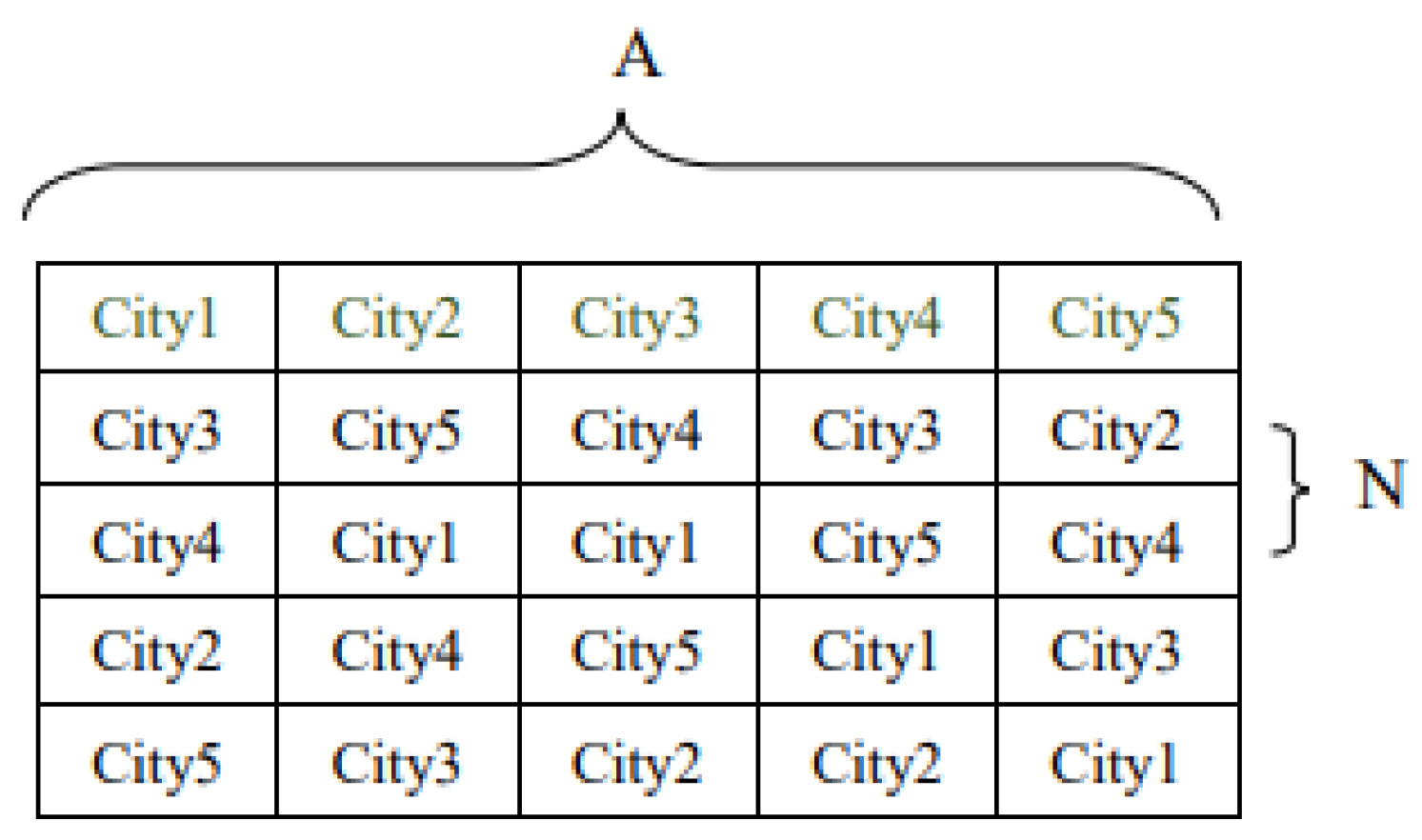
3.2. Biogeography-Based Optimization Algorithm (BBO)

In the biogeographic-based optimization algorithm (BBO) model, each individual of the population is in a different habitat, and the adaptability of the individual in the habitat can be expressed by a Habitat Suitability Index (HSI) [31]. The optimization process deals with one candidate solution for the first HSI, and its optimization level can reflect the advantages and disadvantages of the candidate solution. This phenomenon is caused by the ecological diversity of the habitat, such as temperature, rainfall, species, vegetation, etc. These factors are called Suitability Index Variables (SIV) [32,33] and serve as the variables corresponding to the problem to be optimized.
In this work, the biogeography-based optimization algorithm can be divided into three steps according to the evolution process of the aforementioned factors:
Step 1.
Initialization:
The HSI of N habitats is randomly generated according to Equation (4). One habitat could provide population survival, and each habitat contains D SIV, which represents the composition matrix for all habitats with D dimensional variables.
The SIV composition matrix for all habitats is as follows:
X = X 1 , X 2 , X N
X i = x i 1 , x i 2 x i D
X i j = L j + r a n d o m ( U j L j )
where
  • L j : T h e l o w e r b o u n d o f t h e j d i m e n s i o n a l v a r i a b l e
  • U j : T h e u p p e r b o u n d o f t h e j d i m e n s i o n a l v a r i a b l e
  • X i j : T h e j d i m e n s i o n a l v a r i a b l e o f h a b i t a t X i
Step 2.
Migration:
The size of the I value represents the HSI value of the habitat X i . All habitats are arranged according to their corresponding HSI power reduction. The original habitat X i is re-assigned a new I value. Habitat X 1 has the highest HIS value. The number of species S i in the ordered habitat X i is calculated by:
S i = S m a x i = 1 N
Among them, S m a x represents the maximum number of individuals that the population can accommodate, generally set as the number of habitats N or N + 1 . The immigration rate λ i and emigration rate μ i of habitat X i are calculated by Equations (6) and (7) as follows:
λ i = I ( 1 S i S m a x )
μ i = E ( S i S m a x )
where I is the maximum immigration rate and E is the maximum emigration rate and are equal. The immigration and emigration rates of each habitat are λ and μ , respectively. Based on probability, X i is chosen as the habitat to be moved to and X j is chosen as the habitat to be moved from. Some SIV components are selected from X j to replace the corresponding SIV in X i . Finally, HSI is calculated to evaluate the new habitat’s adaptability.
Step 3.
Mutation:
Habitat X i is selected according to the probability of mutation, and an SIV is randomly generated to replace the SIV in X i . Mutation can improve a habitat with low SIV, thereby increasing the value of SIV. The BBO algorithm first generates N habitats randomly, then chooses the place of immigration and the place of migration according to the probability. Next, the habitat environment is changed according to the mutation probability P m u t e , and iterates repeatedly until the termination condition of the algorithm is satisfied.
The flowchart of the BBO algorithm is shown in Figure 1. In the original BBO algorithm, the mutation probability is generated by a complex calculation based on the number of species. Simon et al. [29,34] found that the optimization results generated by such complex calculations are not superior to simple methods. At present, the mutation probability uses a smaller fixed value. Similar to most intelligent optimization algorithms, the BBO algorithm first generates N habitats randomly, then chooses the place of entry and the place of exit according to the probability of successful migration. It then ensures habitat environment variation according to the mutation probability P m u t e , which iterates repeatedly until the termination condition of the algorithm is satisfied.

3.3. Random Greedy Initialization

For the initial arrangement and combination of cities in the traveling salesman problem, if a random or sequential arrangement is adopted, the reduction in complexity in finding the optimal solution is very limited, and it is easy to fall into the state of a local optimal solution if the greedy method is used. Instead, this paper adopts a random greedy method to eliminate local optimal solutions and also provide fast convergence. An example using the random greedy method for initialization follows.
For example, for the convenience of explaining the principle of the random greedy method, the coordinates of five cities are as shown in Table 2, where the coordinate values are set randomly.
Calculating the distance between cities results in a two-dimensional array City Distance [29], as shown in Table 3:
According to the array value of CityDistance, compare the distance between a city and other cities, and sort the order of cities from small to large, to obtain a two-dimensional array CityOrder, as shown in Figure 2:
After each new city coordinate is entered, the first city acquires the next city by random greedy (with conditions: it must be located in the top N cities and N is recommended to be less than or equal to A W , where all cities are A and W is the best value denominator variable. It is recommended that W be 5, and N is not less than 2) as in Equation (8). As a solution for the trajectory path of all cities, the complete greedy method is not necessarily viable. Note the optimal solution of TSP can also avoid local optimal solutions through random greedy method.
N = 2 , A W < 2 A W , A W 2
d i j = ( X i X j ) 2 ( Y i Y j ) 2
  • d i j : D i s t a n c e f r o m i t o j
  • X i : X a x i s c o o r d i n a t e v a l u e o f c i t y i
  • Y j : Y a x i s c o o r d i n a t e v a l u e o f c i t y j
  • X i : X a x i s c o o r d i n a t e v a l u e o f c i t y i
  • Y j : Y a x i s c o o r d i n a t e v a l u e o f c i t y j

3.4. 2-Opt Algorithm

The 2-opt algorithm is a method for solving the TSP. The principle of 2-opt is to reroute the travel path to remove instances where it crosses over itself. The process of applying the 2-opt algorithm to TSP is as follows: Select two paths from all paths to delete. Change the next hop of one path to the initial node of the other path. Traverse that path in reserve and connect with the next hop of the original path. Then, recalculate the total traveled distance for the new circuit. If the newly generated combination has a shorter path, replace the old combination with a new combination. Otherwise, reject changes and retain the original combination. Taking Figure 3 and Figure 4 as an example, the original circuit is ① → ④ → ② → ③. When 2-Opt is launched, two paths (1,4), (2,3) are deleted. The initial node is selected from one of the deleted paths. In this case (1,4) is selected and this node’s next hop will be changed to node 2 and then continue the path by reversing the direction between node 2 and node 4. Then, the path will continue by connecting to the next hop of the other deleted path, thereby completing the circuit. As shown in Figure 4, the new circuit order is ① → ② → ③ → ④. The length of the new path is then recalculated. If it is shorter than the original circuit, the new path is adopted. Otherwise, the original circuit is retained.

3.5. G2BBO Solving Travel Salesman Problem

When the original biogeographic algorithm is used to solve the traveling salesman problem, it is possible to be trapped in a local optimal solution during later iterations. Therefore, two methods are applied to address this shortcoming in this work. The first is to use greedy-random initialization to obtain an initial travel solution that is closer to the optimal solution. After the migration and mutation of the reasoning algorithm, the 2-opt algorithm is used to improve the circuit path [35], so as to obtain the best solution. Please refer to the flowchart of the improved method in Figure 5. In the Figure, P is the population size and N m a x is the maximum number of iterations.
In the beginning, using the random greedy method to obtain the initial solution of each population, and performed N iterations. In each iteration, the Migration and Mutation of the BBO algorithm are first executed. Each population first applies the BBO standard program to obtain an approximate solution. Next, we optimized the path for each population by the 2-opt algorithm. After each iteration, we sorted the sum of the paths of all populations from small to large. If the minimum path value of this iteration is less than the above value once, we would replace it with the temporary minimum value of the path, and keep it unchanged in the next iteration until the last iteration. The final total path value is the optimal value of the G2BBO algorithm.

4. Experimental Results

The following describes the relevant parameter settings and flow of the experimental process:

4.1. Setting of Experimental Parameters

Using TSP LIB test data sets eil51, eil76, and kroA100, both the original BBO algorithm (BBO) and the improved BBO algorithm (G2BBO) applied greedy-random initialization (GRI) and 2-opt algorithm. The parameters of the BBO algorithm are set as follows:
  • Population Size = 10, Iterations = 1000;
  • Elite retention number = 2, P m o d = 1,
    Maximum migration probability I = 1;
  • Maximum migration probability E = 1;
  • Migration rate = 0.7, Mutation rate = 0.07;
  • Each method runs independently 10 times to obtain the shortest path solution.

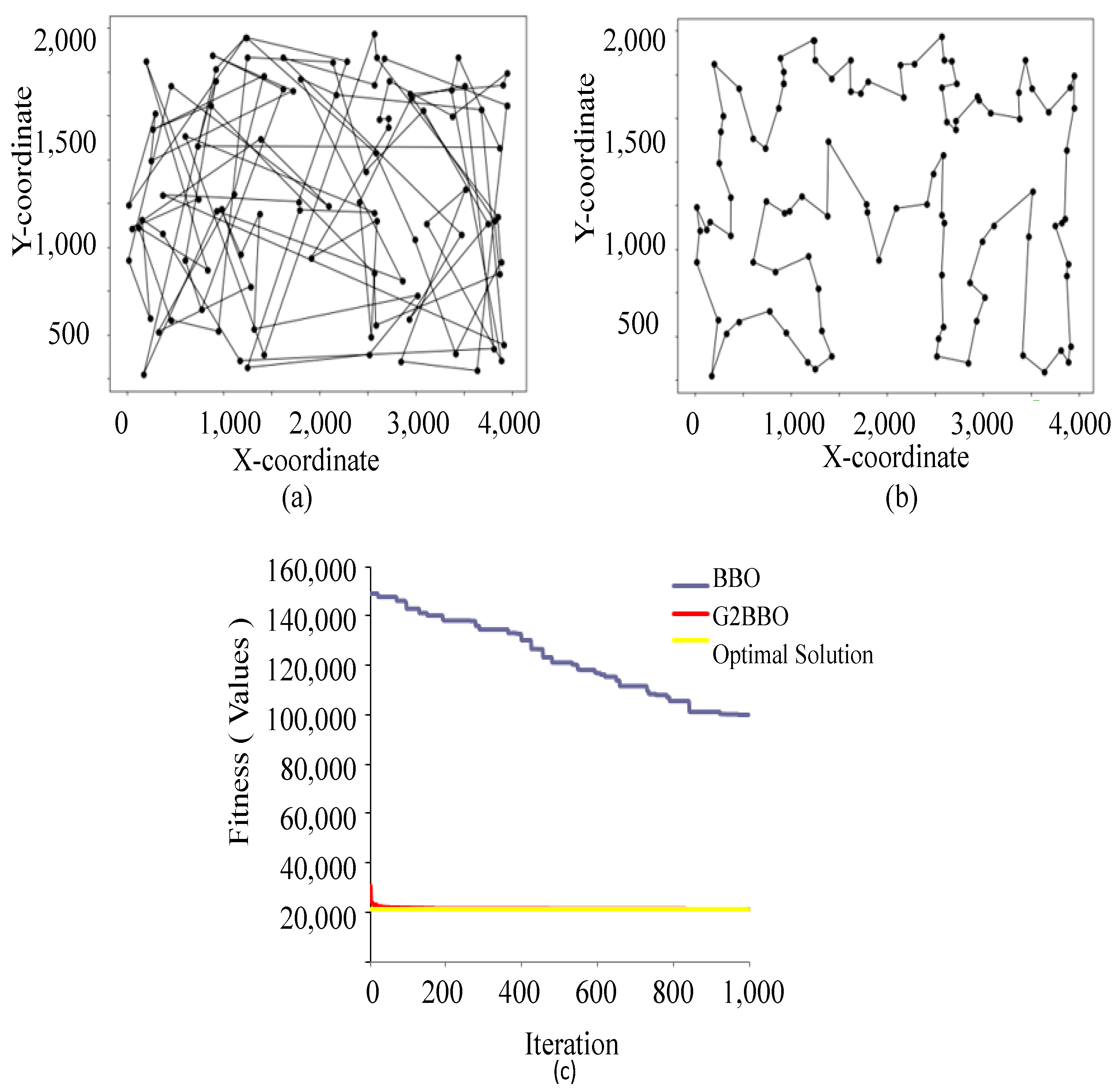
4.2. Analysis of Experimental Results

The original BBO algorithm and the improved BBO algorithm (G2BBO) are used to calculate the TSP test sets (Eil51, Eil76, KroA100) in the following three groups of graphs. In addition to showing the shortest path, the original BBO, improved BBO algorithm (G2BBO), and optimal curve of the data set are compared in the same graph. It can be seen that the distance and therefore performance between the original BBO curve and the optimal curve is quite far. While the curve of the improved BBO algorithm (G2BBO) is very a close fit to the values of the optimal curve, showing that the improved BBO algorithm (G2BBO) results are nearly optimal.
Figure 6a,b illustrate the difference between BBO and G2BBO on the TSPLIB graph instance Eil51 which has 51 cities. In Figure 6c, the BBO algorithm has a clear approach to the optimal solution before 400 iterations. However, after that, it cannot break through the local optimal solution, resulting in slower convergence speed and stagnation. In contrast, the G2BBO algorithm quickly approached the global optimal solution before 10 iterations. G2BBO shows efficiency in solving the TSP path optimal solution.
Figure 7a,b illustrate the difference between BBO and G2BBO on the TSPLIB graph instance Eil76 which has 76 cities. In Figure 7c, the BBO algorithm has a good convergence effect before 600 iterations, but after that, the convergence speed gets slower and slower, and it is unable to break through to the local optimal solution. On the other hand, G2BBO also has a good convergence effect before 10 iterations.
Figure 8a,b illustrate the difference between BBO and G2BBO on the TSPLIB graph instance KroA100 which has 100 cities. In Figure 8, the BBO algorithm has continuous convergence before 800 iterations, but stagnates thereafter, while G2BBO also quickly converges to the global optimal solution before 10 iterations.
Table 4 shows that when the number of city points is less than 100 locations Eil51 (Eil76), the best solution values of these algorithms (BB0 = 974 (1492), G2BBO = 428 (546), MA = 501 (-), DRSO = 432.57 (569.5), GA-JGHO = 429.93 (545.1), BBOEAX = 446.43 (-)) with Optimal = 426 (538). However, after more than 100 locations in the KroA100 dataset where Optimal = 21,282, the G2BBO = 21,294 obviously transcend other algorithms (BB0 = 99,927, DRSO = 21,748.4, GA-GHO = 21,522.7, BBOEAX = 22,549.5). Furthermore, with KroA100in Table 4 the relative error value of the G2BBO algorithm is
| 21294 G 2 B B O 21282 O p t i m a l ) / 21282 O p t i m a l | × 100 = 0.056 %

4.3. Summary

The advantages of G2BBO using a random greedy algorithm to solve TSP include simplicity and ease of implementation. The random greedy algorithm has relatively low time complexity and can effectively help G2BBO stabilize the initial solution to find the approximate solution range of significant instances of TSP. 2-opt is a local search optimization algorithm used to solve the TSP. The 2-opt algorithm is fast and can quickly generate new solutions to find local optimal solutions for TSP. The 2-opt algorithm can improve the initial solution generated by other algorithms because it can find the optimal local solution closer to the optimal global solution. The 2-opt algorithm can easily adjust other optimization problems. Therefore, our method used the greedy algorithm for the initial population and the 2-opt algorithm to improve the local search of G2BBO. The result demonstrates that our method effectively addresses TSP.

5. Conclusions and Future Works

We have presented a novel algorithm “G2BBO” to achieve high efficiency in solving the TSP problems of the three public datasets (Eil51, Eil76, KroA100). In each dataset, G2BBO shows higher performance than the ordinary BBO. Compared to several modern methods such as MA, DROS, GA-JGHO, and BBOEAX, all of the results are very close for datasets with a low number of TSP locations (Eil51, Eil76). With more TSP locations (KroA100), the advantage of G2BBO over other methods is more obvious, since the relative error of G2BBO is at 0.056%. Therefore, we conclude that G2BBO is capable of solving TSP problems well, especially for problems with many locations that are difficult for other methods. For the extended development of G2BBO, it can be applied to model the spread of the COVID-19 virus. The two original characteristics of BBO are migration and mutation, which are apt to measure the spread of the COVID-19 virus. In future work, we will be able to infer a 3D G2BBO algorithm to calculate the optimal 3d path of Starlink data transmission and provide fast internet transmission quality.

Author Contributions

C.-H.T.: Writing—original draft, Data curation, Methodology, Formal analysis, Formal analysis, Visualization. Y.-D.L.: Writing—original draft, Writing—review & editing, Investigation, Formal analysis. C.-H.Y.: Writing—review & editing, Validation, Resources, Supervision. C.-K.W.: Writing—review & editing. L.-C.C.: Validation, Resources, Writing—review & editing, Supervision. P.-J.C.: Project administration, Resources, Validation, Supervision. All authors have read and agreed to the published version of the manuscript.

Funding

This research received no external funding.

Institutional Review Board Statement

Not applicable.

Informed Consent Statement

Not applicable.

Data Availability Statement

Not applicable.

Acknowledgments

The authors would like to thank Michael Chang ([email protected]) for providing proofreading services for this work.

Conflicts of Interest

The authors declare no conflict of interest.

References

  1. Baranidharan, B.; Meidute-Kavaliauskiene, I.; Mahapatra, G.S.; Činčikaitė, R. Assessing the Sustainability of the Prepandemic Impact on Fuzzy Traveling Sellers Problem with a New Fermatean Fuzzy Scoring Function. Sustainability 2022, 14, 16560. [Google Scholar] [CrossRef]
  2. Dell’Amico, M.; Montemanni, R.; Novellani, S. Exact models for the flying sidekick traveling salesman problem. Int. Trans. Oper. Res. 2022, 29, 1360–1393. [Google Scholar] [CrossRef]
  3. Huerta, I.I.; Neira, D.A.; Ortega, D.A.; Varas, V.; Godoy, J.; Asín-Achá, R. Improving the state-of-the-art in the traveling salesman problem: An anytime automatic algorithm selection. Expert Syst. Appl. 2022, 187, 115948. [Google Scholar] [CrossRef]
  4. Salem, I.E.; Mijwil, M.M.; Abdulqader, A.W.; Ismaeel, M.M. Flight-schedule using Dijkstra’s algorithm with comparison of routes findings. Int. J. Electr. Comput. Eng. 2022, 12, 1675. [Google Scholar] [CrossRef]
  5. Watrous, J. On one-dimensional quantum cellular automata. In Proceedings of the IEEE 36th Annual Foundations of Computer Science, Milwaukee, WI, USA, 23–25 October 1995. [Google Scholar]
  6. Laporte, G. The traveling salesman problem: An overview of exact and approximate algorithms. Eur. J. Oper. Res. 1992, 59, 231–247. [Google Scholar] [CrossRef]
  7. Ariani, S.; Santosa, B.; Wiratno, S.E.; Suprianti, R. Analisis Kompleksitas Algoritma Biogeography Based Optimization (BBO) Pada Traveling Salesman Problem (TSP). JASIKA (J. Apl. Sist. Inf. Dan Inform.) 2020, 1, 10–17. [Google Scholar]
  8. Safayenikoo, H.; Nejati, F.; Nehdi, M.L. Indirect Analysis of Concrete Slump Using Different Metaheuristic-Empowered Neural Processors. Sustainability 2022, 14, 10373. [Google Scholar] [CrossRef]
  9. Salehi, A.; Masoumi, B. Solving traveling salesman problem based on biogeography-based optimization and edge assembly cross-over. J. AI Data Min. 2020, 8, 313–329. [Google Scholar]
  10. Al-Taani, A.T.; Al-Afifi, L.M. Solving the Multiple Traveling Salesman Problem Using Memetic Algorithm. Artif. Intell. Evol. 2022, 3, 27–40. Available online: https://ojs.wiserpub.com/index.php/AIE/article/view/1206 (accessed on 1 May 2022). [CrossRef]
  11. Mzili, T.; Riffi, M.E.; Mzili, I.; Dhiman, G. A novel discrete Rat swarm optimization (DRSO) algorithm for solving the traveling salesman problem. Decis. Mak. Appl. Manag. Eng. 2022, 8, 287–299. [Google Scholar] [CrossRef]
  12. Riffi, M.E. Drso: Improved Discrete Rat Swarm Optimization Algorithm (Drso) for Solving the Traveling Salesman Problem. Available online: https://papers.ssrn.com/sol3/papers.cfm?abstract_id=4154967 (accessed on 1 May 2022).
  13. Zhang, P.; Wang, J.; Tian, Z.; Sun, S.; Li, J.; Yang, J. A genetic algorithm with jumping gene and heuristic operators for traveling salesman problem. Appl. Soft Comput. 2022, 127, 109339. [Google Scholar] [CrossRef]
  14. Jena, S.S.; Dash, P.K. A Hybrid Evolutionary Algorithm for Traveling Salesman Problem with Stochastic Distances. Evol. Comput. 2019, 12, 241–255. [Google Scholar]
  15. Singh, P.K.; Dash, P.K. Dynamic Traveling Salesman Problem: An Overview. Math. Model. Eng. Probl. 2019, 6, 309–315. [Google Scholar]
  16. Castellanos, M.R.; Mezura-Montes, E.; Moreno-Perez, J.A. A multi-objective approach to the traveling salesman problem with soft time windows. Soft. Comput. 2018, 22, 1233–1246. [Google Scholar]
  17. de Castro, L.A.; Von Zuben, F.J.; Krohling, R.A. A parallel hybrid genetic algorithm for the traveling salesman problem. IEEE Trans. Cybern. 2018, 48, 2838–2849. [Google Scholar]
  18. Almeida, L.S.; Goerlandt, F.; Pelot, R.; Sörensen, K. A Greedy Randomized Adaptive Search Procedure (GRASP) for the multi-vehicle prize collecting arc routing for connectivity problem. Comput. Oper. Res. 2022, 143, 105804. [Google Scholar] [CrossRef]
  19. Lakhdar, B.; Yahyaoui, K. Solving the Mixed-model Assembly Line Balancing Problem by using a Hybrid Reactive Greedy Randomized Adaptive Search Procedure. In Optimization and Machine Learning: Optimization for Machine Learning and Machine Learning for Optimization; Wiley-ISTE: Hoboken, NJ, USA, 2022; pp. 91–118. [Google Scholar] [CrossRef]
  20. Sun, X.; Chou, P.; Koong, C.S.; Wu, C.C.; Chen, L.R. Optimizing 2-opt-based heuristics on GPU for solving the single-row facility layout problem. Future Gener. Comput. Syst. 2022, 126, 91–109. [Google Scholar] [CrossRef]
  21. Manthey, B.; van Rhijn, J. Improved Smoothed Analysis of 2-Opt for the Euclidean TSP. arXiv 2022, arXiv:2211.16908. [Google Scholar]
  22. Challaf, O.; Chua, S.L.; Foo, L.K. Trip Itinerary Generation with 2-Opt Algorithm. In Proceedings of the 4th International Conference on Advanced Information Science and System, Sanya, China, 25–27 November 2022; pp. 1–5. [Google Scholar]
  23. Shayanfar, H.; Gharehchopogh, F.S. Farmland fertility: A new metaheuristic algorithm for solving continuous optimization problems. Appl. Soft Comput. 2018, 71, 728–746. [Google Scholar] [CrossRef]
  24. Abdollahzadeh, B.; Gharehchopogh, F.S.; Mirjalili, S. African vultures optimization algorithm: A new nature-inspired metaheuristic algorithm for global optimization problems. Comput. Ind. Eng. 2021, 158, 107408. [Google Scholar] [CrossRef]
  25. Abdollahzadeh, B.; Gharehchopogh, F.S.; Khodadadi, N.; Mirjalili, S. Mountain gazelle optimizer: A new nature-inspired metaheuristic algorithm for global optimization problems. Adv. Eng. Softw. 2022, 174, 103282. [Google Scholar] [CrossRef]
  26. Abdollahzadeh, B.; Soleimanian Gharehchopogh, F.; Mirjalili, S. Artificial gorilla troops optimizer: A new nature-inspired metaheuristic algorithm for global optimization problems. Int. J. Intell. Syst. 2021, 36, 5887–5958. [Google Scholar] [CrossRef]
  27. Wang, L.; Cao, Q.; Zhang, Z.; Mirjalili, S.; Zhao, W. Artificial rabbits optimization: A new bio-inspired meta-heuristic algorithm for solving engineering optimization problems. Eng. Appl. Artif. Intell. 2022, 114, 105082. [Google Scholar] [CrossRef]
  28. Naruei, I.; Keynia, F. Wild horse optimizer: A new meta-heuristic algorithm for solving engineering optimization problems. Eng. Comput. 2022, 38 (Suppl. 4), 3025–3056. [Google Scholar] [CrossRef]
  29. Simon, D.; Omran, M.G.; Clerc, M. Linearized biogeography-based optimization with re-initialization and local search. Inf. Sci. 2014, 267, 140–157. [Google Scholar] [CrossRef] [Green Version]
  30. Baniasadi, P.; Foumani, M.; Smith-Miles, K.; Ejov, V. A transformation technique for the clustered generalized traveling salesman problem with applications to logistics. Eur. J. Oper. Res. 2020, 285, 444–457. [Google Scholar] [CrossRef]
  31. Keeley, A.T.; Beier, P.; Keeley, B.W.; Fagan, M.E. Habitat suitability is a poor proxy for landscape connectivity during dispersal and mating movements. Landsc. Urban Plan. 2017, 161, 90–102. [Google Scholar] [CrossRef]
  32. Hadidi, A. A robust approach for optimal design of plate fin heat exchangers using biogeography based optimization (BBO) algorithm. Appl. Energy 2015, 150, 196–210. [Google Scholar] [CrossRef]
  33. Villacreses, G.; Gaona, G.; Martínez-Gómez, J.; Jijón, D.J. Wind farms suitability location using geographical information system (GIS), based on multi-criteria decision making (MCDM) methods: The case of continental Ecuador. Renew. Energy 2017, 109, 275–286. [Google Scholar] [CrossRef]
  34. Ma, H.; Simon, D. Evolutionary Computation with Biogeography-Based Optimization; John Wiley & Sons: Hoboken, NJ, USA, 2017. [Google Scholar]
  35. Akhand, M.; Peya, Z.J.; Sultana, T.; Rahman, M.H. Solving capacitated vehicle routing problem using variant sweep and swarm intelligence. J. Appl. Sci. Eng. 2017, 20, 511–524. [Google Scholar]
Figure 1. BBO (biogeography-based optimization) flowchart.
Sustainability 15 05111 g001
Figure 2. The order of the distance between each city and other cities from small to large.
Sustainability 15 05111 g002
Figure 3. Original path.
Sustainability 15 05111 g003
Figure 4. Updated path via 2-opt.
Sustainability 15 05111 g004
Figure 5. Improved biogeography-based optimization (G2BBO) flowchart.
Sustainability 15 05111 g005
Figure 6. Calculation results for Eil51 from TSPLIB Database. Note: (a) BBO Algorithm (Fitness = 974); (b) G2BBO Algorithm (Fitness = 428); (c) Iterative calculation trend chart of the three algorithms. (Eil51 optimal = 426).
Sustainability 15 05111 g006
Figure 7. Calculation results for Eil76 from TSPLIB Database. Note: (a) BBO Algorithm (Fitness = 1492); (b) G2BBO Algorithm (Fitness = 546); (c) Iterative calculation trend chart of the three algorithms. (Eil76 optimal = 538).
Sustainability 15 05111 g007
Figure 8. Calculation results for KroA100 from TSPLIB Database. Note: (a) BBO Algorithm (Fitness = 99,927); (b) G2BBO Algorithm (Fitness = 21,285); (c) Iterative calculation trend chart of the three algorithms. (KroA100 optimal = 21,282).
Sustainability 15 05111 g008
Table 1. Comparison of the seven algorithms.
AlgorithmInspirationSolution
Farmland Fertility
Algorithm [23]
Farmland fertility
in nature
Solving a continuous
optimization problem
The African vulture
optimization algorithm [24]
African vultures’
lifestyle
Solving large-scale
problems
The mountain gazelle
optimizer [25]
The social life and
hierarchy of wild
mountain gazelles
High-dimensional search
capabilities
The artificial
gorilla troops
optimizer [26]
Gorilla troops’
social intelligence
in nature
Solving onhigh-
dimensional
problems
Artificial rabbits
optimization [27]
The survival strategies
of rabbits in nature
Solving engineering
optimization problems
Wild horse
optimization [28]
The social behavior
of wild horses in nature
Solving problems in
various scientific fields
G2BBO
optimization
Biogeography regarding the migration
of species between different habitats,
as well as the evolution and extinction
of species
Solving large-scale and
multiple objectives
optimization problems
Table 2. X- and Y-Coordinates of the five cities.
CityXY
City 1225490
City 2425100
City 3425650
City 4650570
City 5675200
Table 3. The distance between the five cities.
City DistanceCity 1City 2City 3City 4City 5
City 10438256432535
City 24380550521269
City 32565500239515
City 44325212390371
City 55352695153710
Table 4. Execution results of three TSP test sets for original BBO algorithm, G2BBO algorithm, MA algorithm [10], DRSO algorithm [11], GA-JGHO algorithm [13], BBOEAX algorithm [9].
InstanceOptimalBBOG2BBOMA
[10]
DRSO
[11]
GA-JGHO
[13]
BBOEAX
[9]
eil51426974428501432.57429.93446.43
eil765381492546-569.5545.1-
KroA10021,28299,92721,294-21,748.421,522.7322,549.54
Disclaimer/Publisher’s Note: The statements, opinions and data contained in all publications are solely those of the individual author(s) and contributor(s) and not of MDPI and/or the editor(s). MDPI and/or the editor(s) disclaim responsibility for any injury to people or property resulting from any ideas, methods, instructions or products referred to in the content.

