Article

Assessing Impacts of Land Use and Land Cover (LULC) Change on Stream Flow and Runoff in Rur Basin, Germany

1
Faculty of Science and Technology, Athabasca University, Athabasca, AB T9S 3A3, Canada
2
Department of Earth Sciences, Old Sac Area, Block-C, Ground Floor, Indian Institute of Technology Kanpur, Kanpur 208016, India
3
Institute of Bio- and Geosciences, Agrosphere (IBG-3), Forschungszentrum Jülich GmbH, 52425 Jülich, North Rhine-Westphalia, Germany
*
Authors to whom correspondence should be addressed.
Sustainability 2023, 15(12), 9811; https://doi.org/10.3390/su15129811
Submission received: 13 April 2023 / Revised: 10 June 2023 / Accepted: 15 June 2023 / Published: 20 June 2023
(This article belongs to the Special Issue Climate Change Mitigation and Adaptation in Sustainable Agriculture)

Abstract

:
Understanding the impact of land use/land cover (LULC) change on hydrology is the key to sustainable water resource management. In this study, we used the Soil and Water Assessment Tool (SWAT) to evaluate the impact of LULC change on the runoff in the Rur basin, Germany. The SWAT model was calibrated against the observed data of stream flow and runoff at three sites (Stah, Linnich, and Monschau) between 2000 and 2010 and validated between 2011 and 2015. The performance of the hydrological model was assessed by using statistical parameters such as the coefficient of determination (R2), p-value, r-value, and percentage bias (PBAIS). Our analysis reveals that the average R2 values for model calibration and validation were 0.68 and 0.67 (n = 3), respectively. The impacts of three change scenarios on stream runoff were assessed by replacing the partial forest with urban settlements, agricultural land, and grasslands compared to the 2006 LULC map. The SWAT model captured, overall, the spatio-temporal patterns and effects of LULC change on the stream runoffs despite the heterogeneous runoff responses related to the variable impacts of the different LULC. The results show that LULC change from deciduous forest to urban settlements, agricultural land, or grasslands increased the overall basin runoff by 43%, 14%, and 4%, respectively.

1. Introduction

An increasing population, climate change, and human activities have led to a progressive decrease in per capita water availability. Vörösmarty et al. [1] indicated that the changes in the world population and economic activities will influence the water supply demand relationship much more strongly than climate change over the period from 2000 to 2025. It is estimated that water use has increased 6-fold over the past century and is rising by 1% per year [2]. Anthropogenic activities such as deforestation, agricultural development, and urban development lead to change in LULC, which causes environmental change and has major implications on earth–atmosphere interactions and sustainable development [3,4]. Globally, humans are altering the landscape at an unprecedented rate and many regions have experienced a massive LULC change. However, there is a significant regional variability in the LULC change trends [5]. For instance, there is a decreasing trend in the forested area in the tropical region, while an increasing trend is observed in the temperate region [6,7]. During the 1980–2000 period, more than 55% of the new agricultural land across the tropics came at the expense of intact forests, and another 28% came from disturbed forests [8]. In the period 2010–2015, the forest area declined by 5.5 million hectare per year across the tropics and increased by 2.2 million hectare per year in the temperate region [9].
LULC changes have impacts on the hydrological processes (evapotranspiration, runoff, leaching, infiltration, etc.) and the hydrologic response [10]. Hence, the reliable quantitative estimation and calculation of various hydrological variables such as stream flows, evapotranspiration (ET), ground water level, and spatio-temporal fluctuations under variable basin conditions are very important for water resource management. Many studies have been conducted to quantify the impact of LULC change on stream flow. Zhang et al. [11] reviewed 312 basins worldwide. Their results showed that deforestation due to various reasons (e.g., urbanization, agricultural expansion, wildfires, and insect infestation) caused an increase in annual stream flow for more than 80% of the basins, whereas afforestation had relatively inconsistent effect on the stream flow. Generally, stream flow increases with deforestation whereas it decreases with afforestation [12,13,14,15,16,17]. However, the stream flow response to LULC change can differ significantly from the general trend especially in large basins (>1000 km2), and hence requires closer scrutiny [18,19]. In addition to the LULC, climate change also needs to be accounted for in the hydrological models to understand the hydrological regime of the region.
Key research methodologies to understand LULC change effects on hydrological processes include paired catchment experiments and hydrological modelling. In paired catchment experiments, two similar catchments are chosen for comparison (generally very close to each other). One is made the control catchment and the other various treatments such as afforestation, deforestation, and vegetation change are applied. Brown et al. [20] performed a review of the use of paired catchment studies for determining the changes in water yield due to variation in vegetation at various timescales. They found that the period taken to reach a new balance under permanent land-use change varies considerably. Deforestation treatments reach a new balance more quickly than afforestation ones. Bosch and Hewlett [12] reviewed 94 catchment experiments that monitored the effect of vegetation change on water resources. They found that in most of the cases, water yield is increased as forest cover is reduced, but in some occasional cases of the sparsely vegetated land, an increased forest cover reduces the water yield. It should be noted that there is high variability in the hydrologic response to such deforestation. Sahin and Hall [21] performed a meta-analysis of 145 catchment experiments using fuzzy linear regression to estimate the change in water yield due to the change in different vegetation types such as coniferous and hardwood. They found that a 10% reduction in the cover of conifer-type forest led to an increase in the water yield by about 20–25 mm, while that in eucalyptus type forest increased by only 6 mm. Brath et al. [22] showed that LULC change can affect the peak flow regime and flood frequency in the Samoggia River basin, Italy. Now, hydrological observatories have been set up to study, in detail, the causes of human influence on runoff volumes and water qualities in some basins, such as the Rur basin [23]. However, long-term catchment experiments, although an important method, take more time and are expensive to set up. Particularly, runoff behavior takes a long time to adapt to the vegetation change in catchment experiments [24].
Hydrological models offer a more viable option for quantifying water balance and evaluating land management practices, and play an important role in scaling up field observations and predicting the impacts of LULC changes on basin hydrology in the river basins [25]. Many basin models have been developed in the last three decades, such as Chemicals, Runoff, and Erosion from Agricultural Management Systems (CREAMS) [26]; Erosion Productivity Impact Calculator (EPIC) [27,28]; Agricultural Non-Point Source model (AGNPS) [29]; Soil and Water Assessment tool (SWAT) [30,31,32]; and Hydrologic Simulation Program–Fortran (HSPF) [33]. These basin models are applied for modelling runoff and soil loss prediction, water quality, land-use change effect assessment, and climate change impacts.
Among the foregoing models, the SWAT is physically a semi-distributed model for analyzing the impact of land management practices on water, sediment, and agricultural chemical yields in basins [30,34]. Numerous studies have been conducted using SWAT to evaluate the effect of LULC and basin management scenarios on various aspects of the hydrological cycle. Nie et al. [35] used SWAT to quantify the effect of LULC changes on hydrological components at the sub-basin scale in the upper San Pedro basin. Their results showed that the urbanization was the strongest contributor to the increase in surface runoff and water yield in the study period. In contrast, the replacement of desert scrub/grassland with mesquite was the strongest contributor to the decreased base flow/percolation and contributed to the increased ET. The SWAT model was used for simulating the stream and sediment runoff of Beressa basin in Ethiopia [36]. Their results showed that the basin experienced a significant increase in the stream and sediment runoff due to an increase in farmland and settlement areas. SWAT have been used for simulating stream flow [37], phosphorus export [38], pollutants [39,40], microorganisms [41], trends in frequencies of extreme precipitation and floods [42], greenhouse gas emissions [43,44,45], and water quality [32,46,47] in several catchments in Europe. Several studies showed that SWAT is not very sensible for land-use change, besides ET, simply because the corresponding change in soil parameters is not captured adequately [48,49,50].
Although the SWAT has been used for the effects of LULC changes on sediments, it has not considered the changes in soil properties and slope when LULC changes in the SWAT. The runoff response to the LULC change is a complex function of the slope, soil, vegetation, sensitivity of the landscape to runoff, basin management operations, etc. The Meuse River basin, a highly urbanized basin, is experiencing changes in its hydrological regime due to climate change and LULC change impacts [51]. The Rur River, a tributary of the Meuse River, supports a population of over 5 million by securing a water supply [52]. Despite the importance of LULC changes to the basins, no studies have been reported to quantitatively compare the performance of the widely used SWAT in the Rur basin. Particularly, LULC change could change other hydrological conditions of a basin, such as slope, ponds, and Riparian zones. These changes have not been represented explicitly in the hydrological response units of the SWAT when LULC changes. The influence of LULC change on runoffs can be masked due to multiple sources of uncertainties in the hydrological modelling in a large basin. Therefore, a careful examination in estimating the impacts of LULC changes is needed for managing water resources and evaluating the impacts of LULC changes on water resources. Under some extreme scenarios of LULC changes, the impacts of LULC changes on stream flow and runoffs of the Rur River need to be evaluated. Such a study has not been accomplished before in the Rur basin, and this area is characterized by strong land-use change, e.g., urbanization, reforestation, opencast mines, recultivation, etc. Finally, the Rur basin can be seen as representative of other areas with similar developments.
The main objective of this study is to evaluate the impacts of LULC changes on the stream flow of the Rur River and assess the feasibility of the SWAT model for this basin by performing sensitivity analysis, calibration, and validation. We will design several specific scenarios of LULC changes to represent extreme LULC changes, primarily concerning deforestation, urbanization, and agricultural expansion. We will qualify the response of stream flow and runoff to different LULC change scenarios. Hence, this study will be helpful for the basin managers and will open up new dimensions for various other applications of SWAT in the Rur basin.

2. Materials and Methods

2.1. Study Area

The Rur basin, covering 2354 km2, is located largely in North Rhine-Westphalia (Germany) with small parts also in Belgium (6.7%) and the Netherlands (4.6%) [23]. It lies between the coordinate locations around 6° E–6°40′ N E and 50°10′–50°30′ N (Figure 1) and shows variability in topography, land use, soil type, and meteorological parameters, which are more pronounced when comparing northern and southern parts. The Rur basin and its sub-basins are shown in Figure S1. The elevation and mean annual temperature of the region approximately decline from 680 m to 30 m and 8.5–10.5 °C to 7.0–9.0 °C, respectively, as we move from north to south. Further, the study area is characterized by flat lowland in the northern part which is part of the German–Belgian loess belt consisting of unconsolidated rock deposits of mainly tertiary and quaternary periods. In the northern part, the major soils are Cumulic Anthrosols near the drainage lines and Haplic Luvisols, both with silt loam textures [53]. Soils with a loamy sand texture (Fimic Anthrosols and Dystric Cambisols) are located in the northernmost part of the loess plain (Figure S2). The soil in this region is very productive. Consequently, the dominant land use in the northern part is cropland, with the main crops being winter wheat, sugar beet, and maize (Figure S3). Other important land use includes open-cast lignite mines and urban settlements. This lowland region receives between 650 mm and 900 mm of precipitation annually, of which between 500 and 600 mm/year evaporates. The southern part of the Rur basin belongs to the low mountain range Eifel, which mainly consists of consolidated rocks of the Rhenish Massif from the Paleozoic and Mesozoic. The hard rock terrain, combined with mountainous slopes and very shallow soil layers, causes low infiltration rates, so that the area is at risk of flooding. Further, low temperature in winters cause low ET. Consequently, strong seasonality with a strong runoff response to rainfall events is observed [54]. Mean annual precipitation in the southern region ranges from 1200 mm/yr (windward side of High Fen Mountains) to 700 mm/yr (leeward side). Coniferous forests, deciduous forests, and pastures are dominant parts of the southern region [23]. Coniferous forests (17.6%), deciduous forests (23.8%), and pastures (15.6%) are dominant parts of the southern region. The main crops are winter wheat (WWHT) (13%), sugar beet (SGBT) (12.6%), and maize (CORN) (5.9%). Other important land uses include open-cast lignite mines and urban settlements (5.6%).

2.2. SWAT Model Description

SWAT is a small watershed to river basin-scale model that considers both upland and stream processes and was developed originally by the United States Department of Agricultural Research Service [2,55,56]. In SWAT, a basin is divided into multiple sub-watersheds or sub-basins to incorporate spatial heterogeneity in terms of land use land cover, soil type, and topography. Each sub-basin is divided into areas of homogenous land-use, soil, and slope; these are called hydrologic response units (HRUs) [57]. SWAT can simulate a number of different physical processes, such as snowfall and melt, vadose zone processes (infiltration, evaporation, plant uptake, lateral flows, and percolation), and groundwater flows in a basin [57]. The stream flow and runoffs are predicted separately for each HRU and routed, using a variable channel routing method [58,59], to obtain the total stream flow and runoff at the outlet of a basin. The SWAT model uses the Natural Resource Conservation Service (NRCS) curve number method [60] to relate a calculated runoff curve number (CN) to direct runoff, after taking into account initial abstraction losses and infiltration rates for estimating surface runoff (Qsurf). The fundamental hydrology of a basin in SWAT is based on the following water balance Equation (1), based on mass balance, which calculates the change in soil water content (SWt):
  S W t = S W 0 + i = 1 t R d a y Q s u r f E a W s w e e p W g w  
SWt = final water content in (mm);
SW0 = initial water content in (mm);
t = time in (days);
Rday = precipitation amount on specific days i (mm);
Qsurf = runoff amount on specific days i (mm);
Ea = evapotranspiration amount on day i (mm);
Wsweep = the amount of water percolated into the vadose zones on a day i (mm);
Wgw = return amount of flow on a day i (mm).
Soil Conservation Service (SCS)–Curve Number (CN) approach is an empirical model developed to estimate the rainfall–runoff relationships based on the land use, soil type, and soil hydrologic conditions and slope. CN values range from 0 to 100. A higher CN (e.g., 100 for pavement) means a higher potential of the surface to create runoff, in contrast to lower CN values (e.g., near 0 values for dry soils on very less slop terrain). The equation used for estimating the surface runoff is as follows:
  Q s u r f = R d a y I a 2 R d a y I a + S  
Qsurf is the surface runoff. I a is the initial abstraction and S is the retention parameter. The retention parameter varies spatially due to changes in soils and land use; changes in soil water content are defined as
S = 25.4 1000 C N 10
The retention parameter is defined as (2) where CN = curve number for the day. The initial abstraction I a is commonly approximated as 0.2S. Therefore, Equation (2) becomes
  Q s u r f = R d a y 0.2 S 2 R d a y 0.8 S  
The runoff will only occur when R d a y > I a . The graphical solution of Equation (3) for different curve number values is also well documented in [60].

2.3. Model Input and Setup

Basin delineation is used to divide the basin into smaller sub-basins, called sub-basins with the stream reaches and directions. The digital elevation model is used when the basin delineation and flow directions (upstream and downstream) are decided. Sub-basin numbers are generated and are used as references throughout the SWAT simulation. On the stream network, sub-basin outlets are created, where water accumulates in the sub-basin to become stream flow. In this study, 27 sub-basins were created. The stream network for the Rur basin was delineated using the digital elevation model in the ArcSWAT 2012 software. Figure 2 shows a flowchart of the SWAT model’s implementation.

2.3.1. Land Use and Soil Definition

Land Use definition is performed where the SWAT-supported land-use classes are mapped to the prepared land-use map of the area. In this study, land use data were downloaded from the CORINE land cover data (CLC) website for the year 2006 and categorized into 13 classes (Figure S3) using the ArcSWAT software.
The SWAT model requires different soil textural and physicochemical properties such as soil texture, available water content, hydraulic conductivity, bulk density, and organic carbon content for different layers of each soil type (Neitsch et al., 2011) [61]. The soil data were downloaded from the Food and Agricultural Organization (FAO), US website (Table S1). The soil raster file for the study area was clipped from the global soil raster database downloaded from the FAO website. For soil definition, the soil raster database was downloaded from the Food and Agricultural Organization (FAO) website and a soil map for the area was prepared using the SWAT-supported soil classification. SWAT uses the NRCS CN method to estimate the runoff. Curve numbers are calculated for each combination of land use and soil.

2.3.2. Digital Elevation Model (DEM), Slope, and Hydrological Response Units (HRUs)

The spatially distributed data (GIS input) needed for the Arc SWAT interface include the Digital Elevation Model (DEM), soil data, land use, and stream network layers. Topography was defined by a DEM that describes the elevation of any point in each given area at a specific spatial resolution. The DEM was used to delineate the basin and estimate the sub-basin parameters, such as the slope gradient, slope length of the terrain, and the stream network characteristics such as channel slope, length, and width. Five slope classes were made for this study, as shown in Figure S4. These classes were used in the HRU definition. The slope is an important parameter in estimating the flow rates in the reaches.
The HRUs are the unique combinations of land use, soil, and slope. After the land-use, soil, and slope definition in the SWAT, they are overlaid to create HRUs to account for the spatial heterogeneity of the basin. However, the level of complexity can be adjusted by providing thresholds (in percentage) for the land use, soil, or slope during HRU definition. The greater the value of the threshold, the lesser the number of HRUs. In this study, thresholds of 0%, 5%, and 10% were provided for the land use, soil, and slope, respectively. A total of 758 HRUs were generated in this study. Creating HRUs increases accuracy and complexity by providing a more detailed description of the water balance. In these circumstances, the number of HRUs can be reduced by choosing appropriate thresholds for land use, soil, and slope during HRU definition [61]. Runoff calculations are performed separately for each HRU and then routed to obtain the total runoff for the basin.

2.3.3. Meteorological Data

Weather data include precipitation, temperature, relative humidity, solar radiation, and wind speed. Of these, precipitation, temperature, and relative humidity are the most important data for hydrological modelling. The weather input data are prepared using observed weather data (temperature, relative humidity, and precipitation) in a specific format supported by the SWAT. The locations of three weather stations are listed in Table S2. SWAT provides a weather generator that uses the average weather statistics for interpolations of the missing data between weather stations. For this study, a daily time, and a warm-up period of 6 years were chosen. The simulation was run, and the different output files for reaches, sub-basins, and HRUs were written. SWAT computes hydrological components such as runoff, ET, sediments, nutrients, and other parameters that can be obtained from the TxInOut folder. Weather data and river discharge data were also used for calibration purposes and for the prediction of stream flow. Table S3 shows the sources of different input data with their description.

2.4. Model Sensitivity Analysis, Calibration and Validation, and Performance

2.4.1. Model Sensitivity Analysis

There are two types of sensitivity analysis ‘one at a time’ and ‘global’. In “one at a time” sensitivity analysis, one parameter is selected at a time and its sensitivity is assessed. Spruill et al. (2000) [62] gave a detailed description of the sensitivity analysis results for a ‘one at a time’ selected parameter for daily stream flow, for a catchment in Kentucky, USA. However, the sensitivity of a parameter often depends on the value of some other parameter because the parameters are not necessarily independent. In this study, we have used global sensitivity analysis, analyzing all the parameters for their sensitivity simultaneously. Model parameters depict the catchment properties and the processes in the catchment. A total of 18 model parameters were identified to affect surface runoff from the preliminary literature survey. For instance, Kannan et al. [63] and White et al. [64] described sensitive parameters for surface runoff. These parameters were checked for sensitivity, and, finally, 13 parameters were selected.
Sensitivity is assessed by measuring the change in the output variable with respect to the change in the input parameter. A greater change in the output variable corresponds a to greater sensitivity. Model sensitivity analysis is an important step during the calibration phase for choosing the most sensitive parameters from a bigger pool of potential parameters affecting the output variable. For sensitivity analysis, SWAT-CUP 2012 software was used, incorporating sequential uncertainty fitting (SUFI-2) optimization algorithm, whereby an objective function (g) was chosen (R2 in this study) and initial uncertainty ranges were set for each parameter (in Equation (5)). The upper and lower limit defining the uncertainty band of the parameter was a subset of the absolute ranges provided by SWAT. SUFI-2 uses Latin hypercube sampling [65] to generate as many combinations of parameter values as there are simulations (100 simulations in our case). These parameter values were regressed against the chosen objective function (equation) and a t-test was applied for assessing parameter sensitivities and used for calibration and validation processes.
b j , m i n b j   b j , m a x
where j = 1, m.
g = α + i = 1 m β i b i
where m is the number of parameters.

2.4.2. Model Calibration and Validation

Calibration is the process where the parameter ranges are adjusted in such a way that a good fit is obtained between the observed and simulated time series data for the period chosen as the calibration period. A different time period is chosen as a validation period (having no overlap with the calibration period), with the same parameter values and the number of simulations used as in the final calibrated model. The goodness-of-fit is assessed based on the criteria that maximum observed data points are bracketed in the 95% prediction uncertainty (95 PPU) band (signifying uncertainty in the predicted values) [66]. The fraction of observed data lying in the 95 PPU band is denoted by the p-factor (value of p = 1 being ideal), whereas the thickness of the 95 PPU band (denoted by r-factor) should be as small as possible (value of r close to 0 being ideal) [66]. In the present study, R2, p value, r value, and percentage bias (PBIAS) are used as performance statistics.
After obtaining and processing input data, they were used to calibrate the SWAT model from 2000 to 2010 and then to validate the model from 2011 to 2015. The LULC used in the calibration and validation is taken from CLC 2006. The model calibration procedure is developed based on optimization techniques [67] with the assumption that an optimal set of parameters exists in the model to describe the surface runoff in the Rur basin. The results from these permutations suggested that the set of optimal values of model parameters allowed the model to optimally describe the basin hydrology, in the sense of having the least error between the simulated and the observed surface runoff. Data from three stations were used for calibration and validation following the sequential calibration technique.

2.5. Model Performance Evaluation

The performance of the hydrological model was assessed by using statistical parameters such as the coefficient of determination ( R 2 ), p value, r value, and PBIAS.

2.5.1. Coefficient of Determination (R2)

The degree of correlation between the observed and the simulated values is measured by the R 2 value. R 2   ranges from 0 to 1. An R 2 close to 1 means that observed and simulated data points are in good agreement, whereas a value close to 0 means no agreement. Although R 2 has been widely used in the literature for estimating the “goodness-of-fit” of the hydrological models, it is recommended to supplement the R 2   with other performance statistics because of its sensitivity to outliers and its inability to discern the additive and proportional differences between simulated and observed data points [68]. The expression for R 2 is
  R 2 = i = 1 n O i O a v r P i P a v r i = 1 n O i O a v r 2 n = 1 P i P a v r 2 2
where R 2 is the coefficient of determination, O i the ith observed value, O a v r is the average observed value of the entire period in consideration, P i the ith simulated (modeled) value, P a v r is the average of the simulated values of the entire study period.

2.5.2. p Value and r Value

The goodness-of-fit is assessed based on the criteria that maximum observed data points are bracketed in the 95% prediction uncertainty (95 PPU), calculated at the 2.5 and 97.5 percentiles of the cumulative distribution of the simulated variables to represent the uncertainty in the predicted values. The fraction of observed data lying in the 95 PPU band is denoted by the p-factor (value of p = 1 being ideal). Further, the thickness of the 95 PPU band (denoted by r-factor) should be as small as possible (value of r close to 0 being ideal). A detailed description of p and r values can be found in [66,69].

2.5.3. PBIAS Value

Percentage bias (PBIAS) measures the average tendency of the simulated data to be underestimated or overestimated. During calibration, one tries to achieve lower values of PBIAS. A positive PBIAS value means underestimation whereas a negative PBIAS means overestimation. A value of PBIAS within the range of ±25% is considered to be satisfactory for the runoff simulations [70]. The mathematical expression for the PBIAS value is
PBIAS = 100 × i = 1 n Q m , i Q s , i i = 1 n Q m , i
where Q stands for the hydrological variable, m stands for measured, and s stands for simulated. The above expression is minimized if PBIAS is chosen as the objective function in the SWAT.
For successful calibration and model performance assessment, Moriasi et al. [70] suggested performance statistics such as R2, NS, PBIAS, RSR, etc., and their ranges. However, it should be noted that these ranges are for a monthly time step. Generally, the values of the test statistics deteriorate as the time resolution increases to a daily time step. In this study, simulation was performed at the daily time step and the ranges in [70] are used only as the reference.

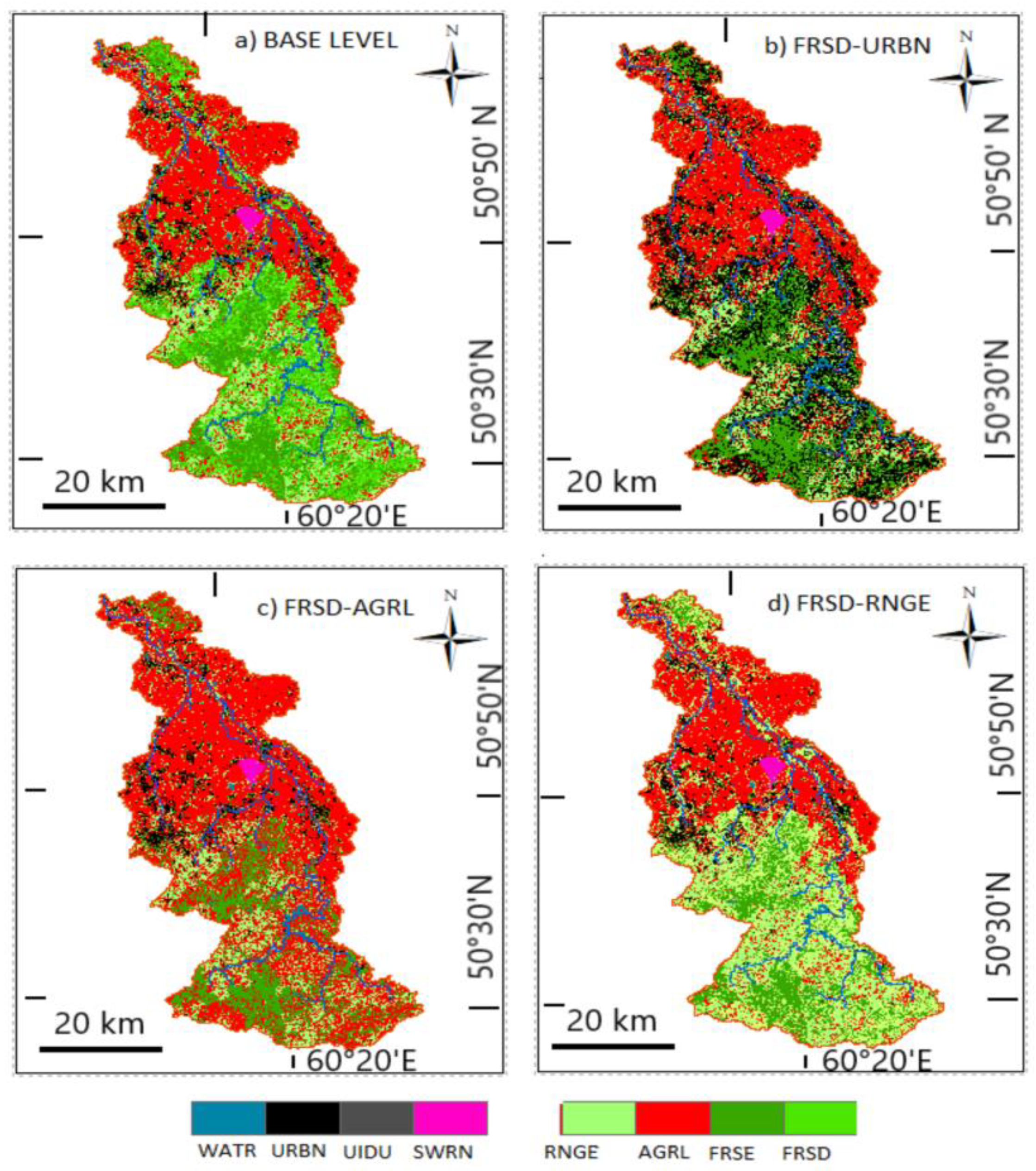
2.6. Scenario Generation and Impacts

Three hypothetical scenarios were constructed to assess the impact of the LULC on stream runoff due to forest area change. The average value of percentage change in the daily runoff was calculated using the following formula:
Q a v e r a g e   o f   d a i l y   p e r c e n t a g e   c h a n g e = i = 1 n Q s c e n a r i o ,   s i m ,   i Q b a s e   l e v e l ,   s i m ,   i × 100 Q b a s e   l e v e l ,   s i m ,   i n
Variability in the percentage change in the daily runoff values was calculated by taking the standard deviation of the percentage change in the daily runoff using the formula
Q v a r i a b i l i t y   = S t d e v   Q p e r c e n t a g e   c h a n g e   i n   r u n o f f   f o r   d a y   i   1   i   n
Q p e r c e n t a g e   c h a n g e   i n   r u n o f f   f o r   i t h   d a y = Q s c e n a r i o ,   s i m ,   i Q b a s e   l e v e l ,   s i m ,   i × 100 Q b a s e   l e v e l ,   s i m ,   i
The percentage change in the average long-term (16 years) runoff was calculated using the formula
Q p e r c e n t a g e   c h a n g e   i n   a v e r a g e   r u n o f f = Q a v e r a g e ,   s c e n a r i o , s i m ,   i Q a v e r a g e , b a s e ,   s i m ,   i Q a v e r a g e , b a s e ,   s i m ,   i × 100
Q a v e r a g e ,   s c e n a r i o , s i m ,   i = i = 1 n Q s c e n a r i o ,   s i m ,   i n  
Q a v e r a g e ,   b a s e   l e v e l , s i m ,   i = i = 1 n Q b a s e   l e v e l ,   s i m ,   i n  

3. Results and Discussion

3.1. Sensitivity Analysis

To identify sensitive parameters, 18 parameters were chosen that affected the surface runoff, reviewing previously calibrated SWAT parameters and documentation from the SWAT manual [61]. Global sensitivity analysis was performed using SWAT-CUP to identify the 13 most sensitive parameters. In this method, the smaller the p-value and greater the absolute value of t-stat, the more sensitive the parameter [71]. Table S4 shows the parameters used for different stations and their ranks at the end of the calibration process for (a) Monschau, (b) Linnich, and (c) Stah, respectively. In order to calibrate the model, the parameter ranges were adjusted to minimize the difference between simulated and observed surface runoff values until an acceptable agreement was attained.
Groundwater delay (GW_delay), curve number (CN2), and base flow factor (ALPHA_BF) were the three most sensitive parameters for all three stations. GW_delay is the time lag between water exiting the soil profile and recharging the aquifer. It depends on the depth of the water table and the hydraulic properties of vadose and ground water zones [61]. Sangrey et al. [72] provides a mathematical relationship between shallow aquifer recharge and GW_delay. Soil evaporation compensation factor (ESCO), average slope length (SLS_SUBBSN), and HRU_SLP (average slope steepness) are the lower sensitivity parameters.

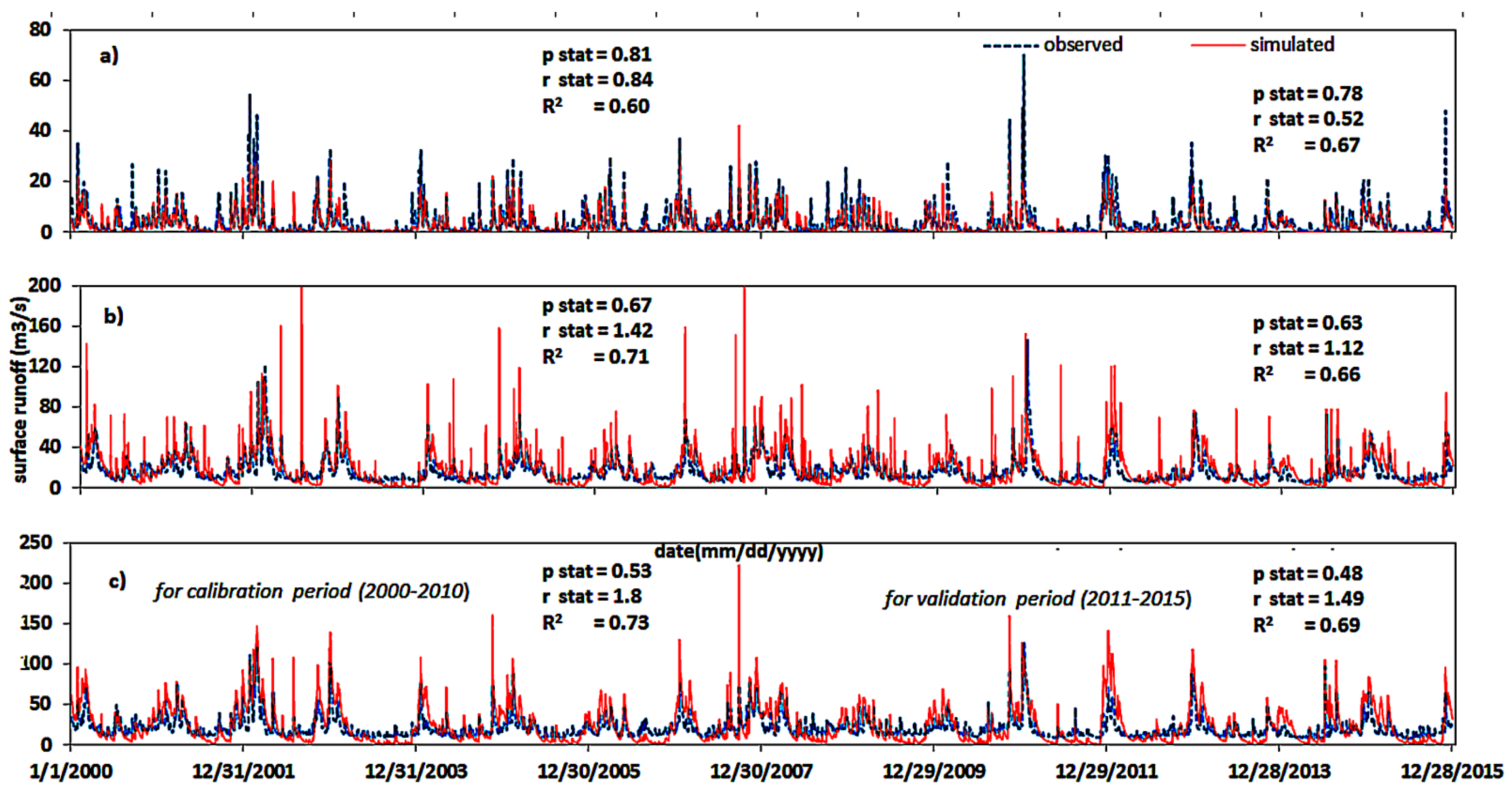
3.2. Model Calibration and Validation

Niraula et al. [73] concluded that the results for the relative change in the stream runoff for the un-calibrated and the single-outlet-calibrated models can vary significantly from the spatially-calibrated models. Hence, spatially-calibrated models should be used to assess the relative change in the stream runoff due to land-use change. Model calibration and validation were carried out for three stations, Stah, Linnich, and Monschau, with the selected parameters after sensitivity analysis using a sequential uncertainty fitting (SUFI-2) algorithm in SWAT-CUP [66]. The model was calibrated for a period of 11 years (2000 to 2010) with a 6-year warm-up period (1994 to 1999) at a daily time step. The model was recalibrated multiple times by changing the lower and upper bounds of the parameter so as to obtain an acceptable agreement between the simulated and observed data. The model was automatically iterated 100 times to obtain the final simulation for the calibration period. The results are given in Table 1.
Figure 3 shows the comparisons of runoffs between simulation results and observed data for the calibration period (2000–2010) and validation period (2011–2015) at all three stations: (a) Monschau, (b) Linnich, and (c) Stah. The model’s performance during calibration and validation was the best at the Monschau station, followed by Linnich and Stah stations. This is evident as the statistical performances are satisfied from the performance statistics (R2, p, and r value) in Figure 4 and Table 1. The key reason for this can be a relative increment in the anthropogenic interventions as we move from the Monschau station in sub-basin 21 to the Stah station in sub-basin 1. From the land-use map, it is evident that the northern part of the basin has much more agricultural and urban land than the southern part of the basin. Water use by the urban population, industries, channel diversions, and dams are not considered in this model but can significantly affect the stream flow in the northern parts of the basin. This can explain why the Monschau station has better performance statistics than the other two stations in regard to both calibrated and validated values. Further, one land-use map was used to calibrate the model for all the years in which the scenario was not a real case. Our simulation was performed at a daily time step, and all absolute values of PBIAS in calibration periods were less than 25%, thus being satisfactory (Table 1). Moriasi et al. [70,74] suggested that an absolute value of PBIAS of up to 25% was satisfactory at a monthly time step. At the basin scale, the result was consistent with other studies (runoff was simulated and compared with the base-level scenario simulation for the individual gauging stations also).

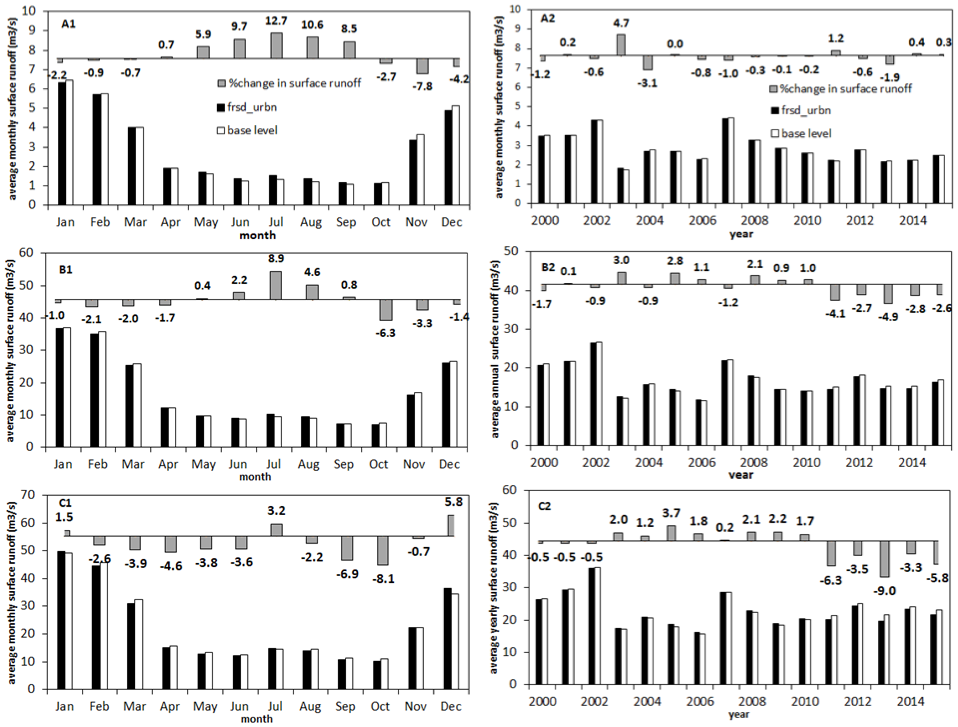
3.3. Effect of LULC Change Scenarios on Stream Flows and Runoffs

Three hypothetical scenarios were constructed to assess the impact of the LULC on stream runoff due to forest area change. Most of these forests were present in parts of the Rur catchment lying in the regions of the western highlands of Germany. Deciduous forests comprise 57.39% of the total forests (coniferous and deciduous combined). For the sake of simplification, the entire deciduous lands in the three scenarios were assumed to be converted to the use of urban settlements, agriculture, or grasslands, respectively (Figure 5). Table S5 shows the description of the three scenarios. The three scenarios were compared with the base-level scenario that was based on the 2006 land-use map. Figure S5 shows that ET presents no changes across any of the scenarios, but there are clear differences regarding percolation, return flow, and runoff between the scenarios. The frsd_urbn scenario has the biggest runoffs, followed by the frsd_agrl scenario and the frsd_rnge scenario.

3.3.1. Forest to Urban Residential

In the frsd_urbn scenario, the simulation results showed that the long-term average runoff increased by 43.05% from 94.48 mm in the base-level scenario to 135.15 mm in the frsd_urbn scenario in the entire basin (Figure 6). This was mainly due to the decrease in percolation from 249.83 mm to 210.61 mm after scenario application. The results also showed that the average runoff in the entire basin increased by 13.47% for the frsd_agrl scenario and 3.45% for the frsd_rnge scenario (Figure 6). This was primarily attributed to decreased percolation in all the scenarios. The decrease in percolation was highest for the frsd_urbn scenario because the impervious surface increased after scenario application. However, the average yearly runoff values decreased for the frsd_urbn scenario at Monschau and Stah while they increased at Linnich station.
Figure 7 shows the time series plot of the relative change (with respect to the base level) in the cumulative stream flow for the period from 2000 to 2015. It was found that there was pronounced seasonality in this scenario. The relative change in the cumulative flow showed a decreasing trend (Figure 7a). This signifies that less water for this scenario will be available from stream flow than that for the base-level scenario at Monschau station. However, at Linnich, the change increased first and then decreased (Figure 7b). There was a peak when the linear trend line fitted in the time series dataset. However, the change showed lower seasonality compared to that at Monschau station. This means that the upstream was more sensitive to seasonality than the downstream. This was consistent with the results in Table 2. In Table 2, the average percentage change in the daily runoff was a positive value of 7.42% at Monschau station while it was a negative value of −6.47% at Linnich station and −9.42% at Stah station. This means that the average daily runoff increased at Monschau station and decreased at the other two stations compared to their baseline level. To obtain a sense of variability in the average daily runoff values, the standard deviation for the daily relative change was calculated to be 56% at Monschau station (%) but 29.87% at Linnich station. This meant that there was a lot of variability observed in the daily runoff values at Monschau station. This can be explained by the fact that when the forests were removed, there was a relatively quick runoff response to rainfalls at a daily time step. The high value of variability can be explained due to the location of the Monschau station in the forested area, with steeper slopes and shallow soil layers.
On the other hand, the annual surface runoff values showed a mixed trend. The average long-term (16 years) runoff change decreased by −0.36% at Monschau station and increased by 2.17% at Linnich station. This is because Linnich station is located in the plane region of the Rur basin, with a slope mostly within the 0–5 % range (Figure S4). The long-term average of the runoff at Stah station became more negative than at Linnich with a value of ~8.97%. The percentage changes in the average monthly and average yearly values were also computed (Figure 8). Percentage change in the monthly values averaged over the period of 2000–2015 showed a positive change in the period April- September compared to the baseline level, while a negative change was observed for the period October–March. The average yearly values showed a mixed trend but a consistent negative relative change from 2011 onwards, although most of these changes were only marginal except for in a few years. Several reasons are attributed to this observation. Firstly, the basin is a complicated, integrated system and the runoff has a different sensitivity to LULC change for different sub-basins. The runoff trend at a certain sub-basin can decrease even if urbanization occurs at the cost of deforestation. There can be a masking effect of some sub-basins [11].
To delve a bit into this issue, the Mann–Kendall test was applied to these three stations. The Mann–Kendall test, as a rank-based non-parametric test, is widely used to test for statistically significant increasing or decreasing trends in the data series [75,76]. The n time series values (Y1, Y2, Y3, …, Yn) are replaced by their relative ranks (S1, S2, S3, …, Sn); the statistical value P of Mann–Kendall test is
P = 1 1 n 1 j = i + 1 n s g n   S j S i  
where sgn(y) = 1 for y > 0;
sgn(y) = 0 for y = 0;
sgn(y) = −1 for y < 0.
If the null hypothesis Ho is true, then Z is approximately normally distributed with
μ = 0;
σ = n (n − 1) (2n + 5)/18.
The z-statistic is therefore
Z = P/ σ 0.5 .
A positive value of p signifies that there is an increasing trend and vice versa [77]. At a significance level of 0.05, if
Z < − 2, then the time series is said to have a statistically significant decreasing trend.
If Z > 2, then the time series is said to have a statistically significant increasing trend.
The z-statistics were calculated (Table S6). The observed values of runoff for the Stah station showed a clear decreasing trend from the years 2007 to 2015 (Figure 9). This was because there was a significant increase in the urban fabric and a decrease in the deciduous forest when comparing the LULC map with the CLC data of 2012 and 2000.

3.3.2. Forest to Agriculture Land Conversion

In the frsd-agrl scenario, the deciduous forest was converted to agricultural land. Thus, agricultural land comprises ~34% of the total basin, with winter wheat, sugar beet, potato, corn, and barley being the dominant crops. The results showed that the long-term average of runoff increased by 13.47% from 94.48 mm in the base-level scenario to 107.21 mm in the frsd_agrl scenario for the entire basin (Figure 6). This was mainly due to the decrease in percolation after scenario application.
Figure 10 shows that the simulated cumulative stream flows increased linearly with little seasonality change at Monschau station and Linnich station. The percentage change of the average daily runoff value was positive for all three stations (Table 2). However, the variability in the relative change of daily runoff was less than that of the frsd_urbn scenario. This implied that the daily runoff was more sensitive to the frsd_urbn scenario than the frsd_agrl scenario in the basin. The long-term average runoff showed an increment at all the three stations (Table 2).
Figure 11 shows the percentage changes in the average monthly and average yearly values that confirm the results of Table 2. The percentage change in the monthly values averaged over the period of from 2000 to 2015 indicated that most of the average monthly runoffs showed either a positive increase (June to September) or a marginal decrease (December to May) in spring and fall. Compared to the frsd_urbn scenario, the long-term averages in the runoff increased for the three scenarios for the entire basin, with exceptional margins across several years. This signifies that more water will be available from stream flow for the frsd_agrl scenario than the base-level scenario. The increase was primarily due to the greater runoff generation of the agricultural land, attributed to the relatively high SCS curve number of the agricultural land as compared to the deciduous forest.

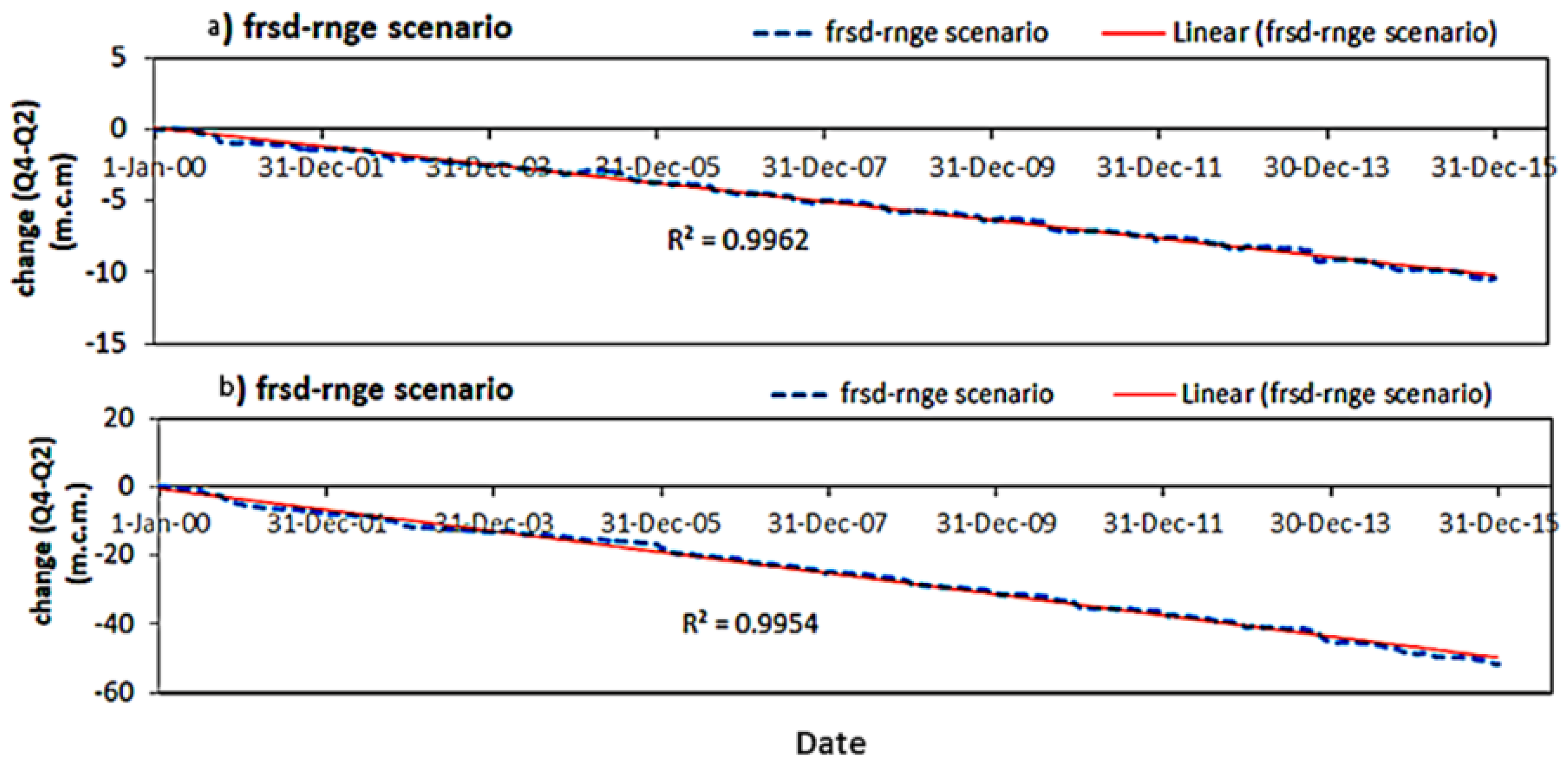
3.3.3. Forest to Perennial Grassland Conversion

In the frsd-rnge scenario, the deciduous forest was converted to perennial grasslands. Grasslands comprise ~16% of the total basin. The results showed that the percentage change in the runoff slightly increased by 3.45% from 94.48 mm in the base-level scenario to 97.74 mm for the entire basin (Figure 6). In Table 2, the percentage change in the average daily runoff was a negative value at all three stations, while the standard deviation in the daily runoff value was positive. The simulated cumulative stream flows decreased over time at the Monschau and Linnich stations compared to the base-level scenario (Figure 12). The long-term average values of the runoff showed a marginal decrease at all three stations. The percentage changes in the average monthly runoff were mostly negative, except for several months in winter at Stah station (Figure 13). The average yearly values showed a consistent decrease for almost all of the years. This was mainly due to the increase in percolation after scenario application compared to the other two scenarios (Figure S5). This implied that the frsd_rnge scenario could reduce the runoff compared to the base level.

3.4. Discussion

The hydrological response to the LULC change is a complex function of the slope, soil, vegetation, sensitivity of the landscape to runoff, basin management operations, etc. The influence of LULC change on runoff can be masked by the complexities found in a large basin [78,79]. Normally, LULC change should not be specific land use or cover. It may involve different land-use changes occurring in mutual ways. For example, for urban growth, the land-use changes may include changes from forest to urban, crop area to urban, and grassland to urban. On the other hand, the greenbelt increase is a land change from buildings to plants. Therefore, the specific changes have several reasons: (1). It is difficult to reflect the reality in the mathematical representation because this needs complex processing in the case of spatial and temporal changes. Thus, LULC changes have to be simplified more or less in any modelling studies. (2). If different LULC changes are considered at the same time, as a result, it will be difficult to explain which land-use change is more important than the other land-use changes. Thus, we think it is better to define a single LULC change to be able to compare the impacts of the different LULC scenarios. (3). The scenarios could be designed for some extreme conditions, such as climate change RCP8.5. Although they are not present in reality, they can somewhat represent the complexity.
The frsd_urbn scenario showed a strong increase in average daily discharge changes compared to the baseline level at the station located in the mountain range, but a decrease at the stations in the lowland agricultural region. Zhang et al. [17] also indicated that upstream forests play an important role in regulating the stream flow through canopy interception, evapotranspiration, and soil interception. In contrast, at the upstream station (Monschau), there were only marginal increases for the frsd_agrl scenario and decreases for the frsd_rnge scenario compared to the base level. The marginal changes in the average daily runoff for the frsd_agrl and the frsd_rnge scenarios can be due to effects of the percolation and return flows where the runoff response of deforestation was not decreased in a sub-basin. For the frsd_urbn scenario, the average long-term (16 years) runoff decreases at the upstream and downstream stations, but marginally increases compared to the base level. In contrast, the average long-term runoff increases for the frsd_agrl scenario and decreases for the frsd_rnge scenarios compared to the base level. These differences in the short- and long-term responses of runoff at the different stations to LULC changes highlight the importance of this study. For example, for the frsd_urbn scenario, a fast increased response of daily and monthly average runoffs implies that urbanization may cause regional flooding and seasonal drying. On the other hand, the grasslands are better able than the forests to prevent runoff and soil erosion. Therefore, the quantitative analysis for the three LULC change scenarios is helpful in developing the best land management practices. In addition, it is found that the runoff response to the LULC change can exhibit a threshold where the change in the surface runoff is not significant unless the threshold in the LULC change is reached. This is consistent with the results by Ghaffari et al. [80]. Further studies remain to be conducted to quantify the threshold for different LULC changes.
SWAT might show a better performance in some Literature [70,74]. It is still not easy for the model to fully capture high peaks and valleys. R2 and r are oversensitive to high extreme values, and insensitive to additive and proportional differences between model prediction and observed data. Therefore, this depends on the dataset quality available rather than monthly or daily data. Generally, the calibration and validation of stream flow are better than runoff, base flow, or water quality. This is mainly because the runoff data, base flow data, and water quality are much less than the steam flows in most basins. In Table 8 of the recent reference [74], for the stream flow, the model performance at the basin scale can be evaluated as “good” if daily values are 0.70 ≤ R2 ≤ 0.85 or “satisfactory” if daily values are 0.50 < R2 < 0.70. For sediment, model performance at the basin scale can be evaluated as “good” if the daily values are 0.65 ≤ R2 ≤ 0.80 or “satisfactory” if the daily values are 0.40 < R2 < 0.65. Therefore, our results should be “good” since we used runoffs for the calibration and validation. In addition, it can be found that the performances in Figure 4 were much better than those in Figure 3. All R2 in Figure 4 are greater than 0.79.
This study is limited in some respects. For instance, the climate change impact and water-use patterns were not accounted for. In a recent study, a climate change simulation and trend analysis of extreme precipitation and floods demonstrated a significant impact on the hydrology of the Rur basin in the mesoscale Rur catchment in western Germany until 2099, using the Statistical Downscaling Model (SDSM) and the SWAT model [42]. Furthermore, the SWAT model does not account for possible changes in soil properties and slopes related to LULC changes and agricultural management, such as grazing, water-use, tillage, and compaction. Particularly, these operations could significantly influence the potential maximum soil retention. In this regard, the current algorithm for the potential maximum soil retention has not represented the importance of vegetation growth and LULC change, and needs to be improved. In addition, the model could be enhanced by including dynamic land-use change, and more data from the ongoing TERENO project (Bogena et al., 2018) [23] could be used for more detailed model evaluation. Finally, the robustness and predictive power of the model can be improved by incorporating the reservoirs, dams, industrial and agricultural water-use data, and climate change scenarios in future studies.

4. Conclusions

Four LULC scenarios were used for assessing the impacts of the LULC changes on stream flow and runoff in Rur basin using the hydrological model SWAT. Three of them comprised deforestation, wherein the deforested land is converted to urban settlements, agriculture, and grasslands, respectively, and one was the baseline scenario. The SWAT model was calibrated for the period 2000–2010 and validated for the period 2011–2015 for all three runoff gauging stations (e.g., Monschau, Linnich, and Stah). The simulation model results showed that the hydrological responses to land use/land cover (LULC) changes in the Rur basin were very different, both for the individual stations (Monschau, Linnich, and Stah) and for different times of the year. The land-use change in the upstream areas can affect more stream flow and runoff than that in the downstream. The relative average daily runoffs were the most sensitive to the partial forest to urban (frsd_urbn) conversion scenario, particularly at the upstream station (Monschau). Therefore, rainfall events lead to higher runoffs or potential local flooding. The long-term average runoff for the entire basin increased by 43% from 95 mm in the base-level scenario to 135 mm in the frsd_urbn scenario due to the percolation decrease. The model also predicted an increase of 12 million cubic meters (m.c.m.) at Monschau and 50 m.c.m. at Linnich in the relative cumulative stream flows and runoffs for the scenario from partial forest converted to agricultural land (frsd_agrl), which may cause soil erosion. In contrast, for the partial forest conversion to rangeland (frsd_rnge), the average daily runoff and annual runoff decreased from −0.1% to −1.93% at all three stations compared to the base-level scenario. This suggested that the presence of more grasslands could reduce runoff and soil erosion. Critically, there are thresholds within the various type and the level LULC conversion wherein a particular sub-basin is not affected until some configuration of land-use change reaches the onset of the threshold. Finally, our study opens up new perspectives for qualifying the impacts of various LULC changes on runoffs in the Rur, and ultimately the Meuse basin, and it provides a powerful tool for runoff, sediment, and implicit nutrient management at the basin scale. Future work needs to account for the impacts of climate change and water-use patterns. The SWAT model should be improved to consider changes in the soil properties and slope when LULC changes in the SWAT.

Supplementary Materials

The following supporting information can be downloaded at: https://www.mdpi.com/article/10.3390/su15129811/s1, Figure S1. Sub-basin boundaries (formed during watershed delineation) and reach network with monitoring stations. Figure S2. Soil classes in the Rur catchment. Figure S3. Land-use map of the Rur catchment classified into 13 land-use classes. Figure S4. Slope classes for the Rur catchment. Figure S5. The evapotranspiration (ET), runoff, percolation, and return flow for different scenarios. Table S1. Characteristics and texture of the SWAT soil classes used in the simulations. Table S2. Weather stations used for temperature, precipitation, and relative humidity. Table S3. Different model inputs, their descriptions, and sources. Table S4. Calibrated parameter for Monschau, Linnich, and Stah stations. The parameters are ordered as per sensitivity rank with the most sensitive parameter at the top. Table S5. Description of all the land use land cover scenarios used in this study. Table S6. Mann–Kendall test results for trend analysis in the average annual observed runoff data (2000–2015).

Author Contributions

Conceptualization, S.S., T.W.M., I.S.S. and J.W.; methodology, T.W.M. and J.W.; formal analysis, T.W.M. and J.W.; investigation, S.S.; data curation, S.S., T.W.M., R.B. and H.B.; writing—original draft, S.S.; writing—review and editing, T.W.M., I.S.S., R.B., H.B. and J.W.; visualization, T.W.M.; supervision, I.S.S. and J.W. All authors have read and agreed to the published version of the manuscript.

Funding

This research received no external funding.

Institutional Review Board Statement

Not applicable.

Informed Consent Statement

Not applicable.

Data Availability Statement

Not applicable.

Acknowledgments

The authors would like to acknowledge the Globalink Research Internship of Mathematics of Information Technology and Complex Systems (MITACS).

Conflicts of Interest

The authors declare no conflict of interest.

References

  1. Vörösmarty, C.J.; Green, P.; Salisbury, J.; Lammers, R.B. Global Water Resources: Vulnerability from Climate Change and Population Growth. Science 2000, 289, 284–288. [Google Scholar] [CrossRef] [PubMed] [Green Version]
  2. UN-Water; UNESCO. United Nations World Water Development Report 2020: Water and Climate Change; UNESCO: Paris, France, 2020. [Google Scholar]
  3. Turner, B.L.; Lambin, E.F.; Reenberg, A. The Emergence of Land Change Science for Global Environmental Change and Sustainability. Proc. Natl. Acad. Sci. USA 2007, 104, 20666–20671. [Google Scholar] [CrossRef] [PubMed] [Green Version]
  4. Turner, B.L.; Skole, D.; Sanderson, S.; Fischer, G.; Fresco, L.; Leemans, R. Land-Use and Land-Cover Change: Science/Research Plan. 1995. Available online: https://asu.elsevierpure.com/en/publications/land-use-and-land-cover-change-scienceresearch-plan-2 (accessed on 14 June 2023).
  5. Wang, J.; Bretz, M.; Dewan, M.A.A.; Aghajani Delavar, M. Machine learning in modelling land use and land cover change (LULCC): Current status, challenges and prospects. Sci. Total Environ. 2022, 822, 153559. [Google Scholar] [CrossRef] [PubMed]
  6. Millennium Ecosystem Assessment. Ecosystems and Human Well-Being: Synthesis; Island Press: Washington, DC, USA, 2005. [Google Scholar]
  7. Lambin, E.F.; Geist, H.J. Land-Use and Land-Cover Change: Local Processes and Global Impacts; Springer Science & Business Media: Berlin/Heidelberg, Germany, 2008. [Google Scholar]
  8. Gibbs, H.K.; Ruesch, A.S.; Achard, F.; Clayton, M.K.; Holmgren, P.; Ramankutty, N.; Foley, J.A. Tropical Forests Were the Primary Sources of New Agricultural Land in the 1980s and 1990s. Proc. Natl. Acad. Sci. USA 2010, 107, 16732–16737. [Google Scholar] [CrossRef] [Green Version]
  9. Keenan, R.J.; Reams, G.A.; Achard, F.; de Freitas, J.V.; Grainger, A.; Lindquist, E. Dynamics of Global Forest Area: Results from the FAO Global Forest Resources Assessment 2015. For. Ecol. Manag. 2015, 352, 9–20. [Google Scholar] [CrossRef]
  10. Welde, K.; Gebremariam, B. Effect of Land Use Land Cover Dynamics on Hydrological Response of Watershed: Case Study of Tekeze Dam Watershed, Northern Ethiopia. Int. Soil Water Conserv. Res. 2017, 5, 1–16. [Google Scholar] [CrossRef]
  11. Zhang, M.; Liu, N.; Harper, R.; Li, Q.; Liu, K.; Wei, X.; Ning, D.; Hou, Y.; Liu, S. A Global Review on Hydrological Responses to Forest Change across Multiple Spatial Scales: Importance of Scale, Climate, Forest Type and Hydrological Regime. J. Hydrol. 2017, 546, 44–59. [Google Scholar] [CrossRef] [Green Version]
  12. Bosch, J.M.; Hewlett, J.D. A Review of Catchment Experiments to Determine the Effect of Vegetation Changes on Water Yield and Evapotranspiration. J. Hydrol. 1982, 55, 3–23. [Google Scholar] [CrossRef]
  13. David, J.S.; Henriques, M.O.; David, T.S.; Tomé, J.; Ledger, D.C. Clearcutting Effects on Streamflow in Coppiced Eucalyptus Globulus Stands in Portugal. J. Hydrol. 1994, 162, 143–154. [Google Scholar] [CrossRef]
  14. Wu, W.; Hall, C.A.S.; Scatena, F.N. Modelling the Impact of Recent Land-Cover Changes on the Stream Flows in Northeastern Puerto Rico. Hydrol. Process. Int. J. 2007, 21, 2944–2956. [Google Scholar] [CrossRef]
  15. Bi, H.; Liu, B.; Wu, J.; Yun, L.; Chen, Z.; Cui, Z. Effects of Precipitation and Land use on Runoff during the Past 50 Years in a Typical Watershed in Loess Plateau, China. Int. J. Sediment Res. 2009, 24, 352–364. [Google Scholar] [CrossRef]
  16. Zhang, X.; Fan, J.; Cheng, G. Modelling the Effects of Land-Use Change on Runoff and Sediment Yield in the Weicheng River Watershed, Southwest China. J. Mt. Sci. 2015, 12, 434–445. [Google Scholar] [CrossRef]
  17. Zhang, M.; Wei, X. Deforestation, Forestation, and Water Supply. Science 2021, 371, 990–991. [Google Scholar] [CrossRef] [PubMed]
  18. Ring, P.J.; Fisher, I.H. The Effects of Changes in Land Use on Runoff from Large Catchments in the Upper Macintyre Valley, NSW. In Hydrology and Water Resources Symposium 1985: Preprints of Papers; Institution of Engineers: Barton, Australia, 1985; pp. 153–158. [Google Scholar]
  19. Costa, M.H.; Botta, A.; Cardille, J.A. Effects of Large-Scale Changes in Land Cover on the Discharge of the Tocantins River, Southeastern Amazonia. J. Hydrol. 2003, 283, 206–217. [Google Scholar] [CrossRef]
  20. Brown, A.E.; Zhang, L.; McMahon, T.A.; Western, A.W.; Vertessy, R.A. A Review of Paired Catchment Studies for Determining Changes in Water Yield Resulting from Alterations in Vegetation. J. Hydrol. 2005, 310, 28–61. [Google Scholar] [CrossRef]
  21. Sahin, V.; Hall, M.J. The Effects of Afforestation and Deforestation on Water Yields. J. Hydrol. 1996, 178, 293–309. [Google Scholar] [CrossRef]
  22. Brath, A.; Montanari, A.; Moretti, G. Assessing the Effect on Flood Frequency of Land Use Change via Hydrological Simulation (with Uncertainty). J. Hydrol. 2006, 324, 141–153. [Google Scholar] [CrossRef]
  23. Bogena, H.R.; Montzka, C.; Huisman, J.A.; Graf, A.; Schmidt, M.; Stockinger, M.; Von Hebel, C.; Hendricks-Franssen, H.J.; Van der Kruk, J.; Tappe, W. The TERENO-Rur Hydrological Observatory: A Multiscale Multi-Compartment Research Platform for the Advancement of Hydrological Science. Vadose Zone J. 2018, 17, 1–22. [Google Scholar] [CrossRef]
  24. Vertessy, R.A. The Impacts of Forestry on Streamflows: A Review. In Proceedings of the Second Forest Erosion Workshop on Forest Management for Water Quality and Quantity, Warburton, Australia, 4–6 May 1999; Croke, J., Lane, P., Eds.; Report 99/6. CRC for Catchment Hydrology: Melbourne, Australia, 1999; pp. 91–108. [Google Scholar]
  25. Niehoff, D.; Fritsch, U.; Bronstert, A. Land-Use Impacts on Storm-Runoff Generation: Scenarios of Land-Use Change and Simulation of Hydrological Response in a Meso-Scale Catchment in SW-Germany. J. Hydrol. 2002, 267, 80–93. [Google Scholar] [CrossRef]
  26. Knisel, W.G. CREAMS: A Field Scale Model for Chemicals, Runoff, and Erosion from Agricultural Management Systems; U.S. Department of Agriculture, Conservation Research Report No. 26; Department of Agriculture, Science and Education Administration: Washington, DC, USA, 1980. [Google Scholar]
  27. Williams, J.R. The Erosion-Productivity Impact Calculator (EPIC) Model: A Case History. Philos. Trans. R. Soc. Lond. Ser. B Biol. Sci. 1990, 329, 421–428. [Google Scholar]
  28. Izaurralde, R.C.; Williams, J.R.; McGill, W.B.; Rosenberg, N.J.; Jakas, M.C.Q. Simulating Soil C Dynamics with EPIC: Model Description and Testing against Long-Term Data. Ecol. Model. 2006, 192, 362–384. [Google Scholar] [CrossRef]
  29. Young, R.A.; Onstad, C.A.; Bosch, D.D.; Anderson, W.P. AGNPS: A Nonpoint-Source Pollution Model for Evaluating Agricultural Watersheds. J. Soil Water Conserv. 1989, 44, 168–173. [Google Scholar]
  30. Arnold, J. SWAT-Soil and Water Assessment Tool; USDA NAL: Beltsville, MD, USA, 1994. [Google Scholar]
  31. Arnold, J.G.; Moriasi, D.N.; Gassman, P.W.; Abbaspour, K.C.; White, M.J.; Srinivasan, R.; Santhi, C.; Harmel, R.D.; van Griensven, A.; Van Liew, M.W.; et al. SWAT: Model use, calibration, and validation. Am. Soc. Agric. Biol. Eng. 2012, 55, 1491–1508. [Google Scholar]
  32. Shrestha, N.K.; Wang, J. Water Quality Management of a Cold Climate Region Watershed in Changing Climate. J. Environ. Inform. 2020, 35, 56–80. [Google Scholar] [CrossRef]
  33. Bicknell, B.R.; Imhoff, J.C.; Kittle, J.L.; Donigian, A.S.; Johanson, R.C. Hydrological Simulation Program–Fortran (HSPF): User’s Manual for Release 12; National Exposure Research Laboratory, US Environmental Protection Agency: Athens, GA, USA, 2001. [Google Scholar]
  34. Shrestha, N.K.; Wang, J. Predicting Sediment Yield and Transport Dynamics of a Cold Climate Region Watershed in Changing Climate. Sci. Total Environ. 2018, 625, 1030–1045. [Google Scholar] [CrossRef]
  35. Nie, W.; Yuan, Y.; Kepner, W.; Nash, M.S.; Jackson, M.; Erickson, C. Assessing Impacts of Landuse and Landcover Changes on Hydrology for the Upper San Pedro Watershed. J. Hydrol. 2011, 407, 105–114. [Google Scholar] [CrossRef]
  36. Worku, T.; Khare, D.; Tripathi, S.K. Modeling Runoff–Sediment Response to Land Use/Land Cover Changes Using Integrated GIS and SWAT Model in the Beressa Watershed. Environ. Earth Sci. 2017, 76, 550. [Google Scholar] [CrossRef]
  37. Piniewski, M.; Szcześniak, M.; Kardel, I.; Berezowski, T.; Okruszko, T.; Srinivasan, R.; Schuler, D.V.; Kundzewicz, Z.W. Hydrological Modelling of the Vistula and Odra River Basins Using SWAT. Hydrol. Sci. J. 2017, 62, 1266–1289. [Google Scholar] [CrossRef]
  38. Nasr, A.; Bruen, M.; Jordan, P.; Moles, R.; Kiely, G.; Byrne, P. A Comparison of SWAT, HSPF and SHETRAN/GOPC for Modelling Phosphorus Export from Three Catchments in Ireland. Water Res. 2007, 41, 1065–1073. [Google Scholar] [CrossRef] [Green Version]
  39. Qiao, P.; Wang, S.; Li, J.; Zhao, Q.; Wei, Y.; Lei, M.; Yang, J.; Zhang, Z. Process, influencing factors, and simulation of the lateral transport of heavy metals in surface runoff in a mining area driven by rainfall: A review. Sci. Total Environ. 2023, 857, 159119. [Google Scholar] [CrossRef]
  40. Du, X.; Shrestha, N.K.; Wang, J. Integrating organic chemical simulation module into SWAT model with application for PAHs simulation in Athabasca oil sands region, Western Canada. Environ. Model. Softw. 2019, 111, 432–443. [Google Scholar] [CrossRef]
  41. Meshesha, T.W.; Wang, J.; Melaku, N.D. A modified hydrological model for assessing effect of pH on fate and transport of Escherichia coli in the Athabasca River basin. J. Hydrol. 2020, 582, 124513. [Google Scholar] [CrossRef]
  42. Eingrüber, N.; Korres, W. Climate change simulation and trend analysis of extreme precipitation and floods in the mesoscale Rur catchment in western Germany until 2099 using Statistical Downscaling Model (SDSM) and the Soil & Water Assessment Tool (SWAT model). Sci. Total Environ. 2022, 838, 155775. [Google Scholar]
  43. Wagena, M.B.; Bock, E.M.; Sommerlot, A.R.; Fuka, D.R.; Easton, Z.M. Development of a nitrous oxide routine for the SWAT model to assess greenhouse gas emissions from agroecosystems. Environ. Model. Softw. 2017, 89, 131–143. [Google Scholar] [CrossRef] [Green Version]
  44. Gao, X.; Ouyang, W.; Lin, C.; Wang, K.; Hao, F.; Hao, X.; Lian, Z. Considering atmospheric N2O dynamic in SWAT model avoids the overestimation of N2O emissions in river network. Water Res. 2020, 174, 115624. [Google Scholar] [CrossRef]
  45. Bhanja, S.N.; Wang, J. Estimating influences of environmental drivers on soil heterotrophic respiration in the Athabasca River Basin, Canada. Environ. Pollut. 2020, 257, 113630. [Google Scholar] [CrossRef]
  46. Glavan, M.; White, S.; Holman, I.P. Evaluation of River Water Quality Simulations at a Daily Time Step–Experience with SWAT in the Axe Catchment, UK. CLEAN–Soil Air Water 2011, 39, 43–54. [Google Scholar] [CrossRef]
  47. Meshesha, T.W.; Wang, J.; Melaku, N.D. Modelling spatiotemporal patterns of water quality and its impacts on aquatic ecosystem in the cold climate region of Alberta, Canada. J. Hydrol. 2020, 587, 124952. [Google Scholar] [CrossRef]
  48. Romanowicz, A.A.; Vanclooster, M.; Rounsevell, M.; La Junesse, I. Sensitivity of the SWAT Model to the Soil and Land Use Data Parametrisation: A Case Study in the Thyle Catchment, Belgium. Ecol. Model. 2005, 187, 27–39. [Google Scholar] [CrossRef]
  49. Malagò, A.; Pagliero, L.; Bouraoui, F.; Franchini, M. Comparing Calibrated Parameter Sets of the SWAT Model for the Scandinavian and Iberian Peninsulas. Hydrol. Sci. J. 2015, 60, 949–967. [Google Scholar] [CrossRef] [Green Version]
  50. Bärlund, I.; Kirkkala, T.; Malve, O.; Kämäri, J. Assessing SWAT Model Performance in the Evaluation of Management Actions for the Implementation of the Water Framework Directive in a Finnish Catchment. Environ. Model. Softw. 2007, 22, 719–724. [Google Scholar] [CrossRef]
  51. Hurkmans, R.T.W.L.; Terink, W.; Uijlenhoet, R.; Moors, E.J.; Troch, P.A.; Verburg, P.H. Effects of Land Use Changes on Streamflow Generation in the Rhine Basin. Water Resour. Res. 2009, 45, W06405. [Google Scholar] [CrossRef] [Green Version]
  52. Bode, H.; Evers, P.; Albrecht, D.R. Integrated Water Resources Management in the Ruhr River Basin, Germany. Water Sci. Technol. 2003, 47, 81–86. [Google Scholar] [CrossRef]
  53. Korres, W.; Reichenau, T.G.; Schneider, K. Patterns and scaling properties of surface soil moisture in an agricultural landscape: An ecohydrological modeling study. J. Hydrol. 2013, 498, 89–102. [Google Scholar] [CrossRef] [Green Version]
  54. Rudi, J.; Pabel, R.; Jager, G.; Koch, R.; Kunoth, A.; Bogena, H. Multiscale analysis of hydrologic time series data using the Hilbert–Huang transform. Vadose Zone J. 2010, 9, 925–942. [Google Scholar] [CrossRef] [Green Version]
  55. Arnold, J.G.; Srinivasan, R.; Muttiah, R.S.; Williams, J.R. Large area hydrologic modeling and assessment part I: Model development. J. Am. Water Resour. Assoc. 1998, 34, 73–89. [Google Scholar] [CrossRef]
  56. Gassman, P.W.; Reyes, M.R.; Green, C.H.; Arnold, J.G. The Soil and Water Assessment Tool: Historical Development, Applications, and Future Research Directions. Trans. ASABE 2007, 50, 1211–1250. [Google Scholar] [CrossRef] [Green Version]
  57. Wang, J.; Shrestha, N.K.; Aghajani Delavar, M.; Worku, M.T.; Bhanja, S.N. Modelling Watershed and River Basin Processes in Cold Climate Regions: A Review. Water 2021, 13, 518. [Google Scholar] [CrossRef]
  58. Williams, J.R.; Hann, R.W. Hymo, A problem-oriented computer language for building hydrologic models. Water Resour. Res. 1972, 8, 79–86. [Google Scholar] [CrossRef]
  59. Williams, J.R.; Hann, R.W. HYMO: Problem-Oriented Computer Language for Hydrologic Modeling: Users Manual; Agricultural Research Service, US Department of Agriculture, Southern Region: Washington, DC, USA, 1973; Volume 9. [Google Scholar]
  60. Biesbrouck, B.; Wyseure, G.; Van Orschoven, J.; Feyen, J. AVSWAT2000. Course; Laboratory for Soil and Water Management (LSWM), Catholic University of Leuven: Leuven, Belgium, 2002. [Google Scholar]
  61. Neitsch, S.L.; Arnold, J.G.; Kiniry, J.R.; Williams, J.R. Soil and Water Assessment Tool Theoretical Documentation (Version 2009); Texas Water Research Resources Institute, Texas A&M University: College Station, TX, USA, 2011. [Google Scholar]
  62. Spruill, C.A.; Workman, S.R.; Joseph, L.; Taraba, T.L. Simulation of Daily and Monthly Stream Discharge From Small Watersheds Using the SWAT Model. Transactions of the ASAE. Am. Soc. Agric. Eng. 2000, 43, 1431–1439. [Google Scholar] [CrossRef]
  63. Kannan, N.; White, S.M.; Worrall, F.; Whelan, M.J. Sensitivity analysis and identification of the best evapotranspiration and runoff options for hydrological modeling in SWAT-2000. J. Hydrol. 2007, 332, 456–466. [Google Scholar] [CrossRef]
  64. White, K.L.; Chaubey, I. Sensitivity analysis, calibration, and validations for a multisite and multivariable SWAT model. J. Am. Water Resour. Assoc. 2005, 41, 1077–1089. [Google Scholar] [CrossRef]
  65. McKay, M.D.; Beckman, R.J.; Conover, W.J. Comparison of Three Methods for Selecting Values of Input Variables in the Analysis of Output from a Computer Code. Technometrics 1979, 21, 239–245. [Google Scholar]
  66. Abbaspour, K.C.; Yang, J.; Maximov, I.; Siber, R.; Bogner, K.; Mieleitner, J.; Zobrist, J.; Srinivasan, R. Modelling hydrology and water quality in the pre-alpine/alpine Thur watershed using SWAT. J. Hydrol. 2007, 333, 413–430. [Google Scholar] [CrossRef]
  67. Guo, H.; Hu, Q.; Jaing, T. Annual and seasonal streamflow responses to climate and land-cover changes in the Poyang Lake basin, China. J. Hydrol. 2008, 355, 106–122. [Google Scholar] [CrossRef]
  68. Legates, D.R.; McCabe, G.J. Evaluating the use of “goodness-of-fit” measures in hydrologic and hydroclimatic model validation. Water Resour. Res. 1999, 35, 233–241. [Google Scholar] [CrossRef]
  69. Abbaspour, K.C.; Rouholahnejad, E.; Vaghefi, S.; Srinivasan, R.; Yang, H.; Kløve, B. A continental-scale hydrology and water quality model for Europe: Calibration and uncertainty of a high-resolution large-scale SWAT model. J. Hydrol. 2015, 524, 733–752. [Google Scholar] [CrossRef] [Green Version]
  70. Moriasi, D.N.; Arnold, J.G.; Van Liew, M.W.; Bingner, R.L.; Harmel, R.D.; Veith, T.L. Model Evaluation Guidelines for Systematic Quantification of Accuracy in Watershed Simulations. Trans. ASABE 2007, 50, 885–900. [Google Scholar] [CrossRef]
  71. Abbaspour, K.C. Swat-Cup 2012: SWAT Calibration and Uncertainty Program—A User Manual; Eawag Swiss Federal Institute of Aquatic Science and Technology: Dübendorf, Switzerland, 2013. [Google Scholar]
  72. Sangrey, D.A.; Harrop-Williams, K.O.; Klaiber, J.A. Predicting Ground-Water Response to Precipitation. J. Geotech. Eng. 1984, 110, 957–975. [Google Scholar] [CrossRef]
  73. Niraula, R.; Meixner, T.; Norman, L.M. Determining the Importance of Model Calibration for Forecasting Absolute/Relative Changes in Streamflow from LULC and Climate Changes. J. Hydrol. 2015, 522, 439–451. [Google Scholar] [CrossRef]
  74. Moriasi, D.N.; Gitau, M.W.; Pai, N.; Daggupati, P. Hydrologic and water quality models: Performance measures and evaluation criteria. Trans. ASABE 2015, 58, 1763–1785. [Google Scholar]
  75. Kendall, M.G. Rank Correlation Methods; Griffin: Santa Barbara, CA, USA, 1948. [Google Scholar]
  76. Mann, H.B. Nonparametric tests against trend. Econom. J. Econom. Soc. 1945, 13, 245–259. [Google Scholar] [CrossRef]
  77. Sheng, Y.; Pilon, P.; Cavadias, G. Power of the Mann–Kendall and Spearman’s rho tests for detecting monotonic trends in hydrological series. J. Hydrol. 2002, 259, 254–271. [Google Scholar]
  78. Wagner, P.D.; Kumar, S.; Schneider, K. An Assessment of Land Use Change Impacts on the Water Resources of the Mula and Mutha Rivers Catchment Upstream of Pune, India. Hydrol. Earth Syst. Sci. 2013, 17, 2233–2246. [Google Scholar] [CrossRef] [Green Version]
  79. Marhaento, H.; Booij, M.J.; Rientjes, T.H.M.; Hoekstra, A.Y. Attribution of Changes in the Water Balance of a Tropical Catchment to Land Use Change Using the SWAT Model. Hydrol. Process. 2017, 31, 2029–2040. [Google Scholar] [CrossRef]
  80. Ghaffari, G.; Keesstra, S.; Ghodousi, J.; Ahmadi, H. SWAT-Simulated Hydrological Impact of Land-Use Change in the Zanjanrood Basin, Northwest Iran. Hydrol. Process. Int. J. 2010, 24, 892–903. [Google Scholar] [CrossRef]
Figure 1. Study area map of Rur basin located in North-Rhine Westphalia, Germany. Digital elevation model with stream networks and gauging stations (e.g., Stah, Linnich, and Monschau) for stream runoff measurements (marked with a red star) are shown.
Sustainability 15 09811 g001
Figure 2. Methodological framework for this study (modified from [36]).
Sustainability 15 09811 g002
Figure 3. Model calibration (in the period 2000–2010) and validation (in the period 2011–2015) for all three stations: (a) Monschau, (b) Linnich, and (c) Stah.
Sustainability 15 09811 g003
Figure 4. Correlations between observed vs. simulated runoff values for the three stations: (A) Monschau, (B) Linnich, and (C) Stah.
Sustainability 15 09811 g004
Figure 5. Land-use map of different scenarios: (a) base-level scenario, (b) deciduous forests (frsd) to urban residential area (urbn) conversions, (c) deciduous forests (frsd) to agricultural area (agrl), and (d) deciduous forests (frsd) to grasslands (rnge).
Sustainability 15 09811 g005
Figure 6. The percentage change in the runoff, percolation, and return flow with respect to the baseline scenario for different scenarios.
Sustainability 15 09811 g006
Figure 7. The change in the simulated cumulative stream flows in million cubic meters (m.c.m) for the forest-urban scenario with respect to the base-level scenario at (a) Monschau and (b) Linnich. Q1–Q2 is the simulated cumulative stream flow for frsd-urbn scenario.
Sustainability 15 09811 g007
Figure 8. The relative changes in the average monthly runoff (A1,B1,C1) and average annual runoff (A2,B2,C2) for the stations Monschau represented by (A), Linnich (B), and Stah (C). All graphs in this figure are for frsd-urbn scenario.
Sustainability 15 09811 g008
Figure 9. Linear decreasing trend from 2007 to 2015 in the observed runoff data of Stah.
Sustainability 15 09811 g009
Figure 10. The change in the simulated cumulative stream flows in million cubic meters (m.c.m.) for the forest-agriculture scenario, with respect to the base-level scenario at (a) Monschau and (b) Linnich. Q3–Q2 is the simulated cumulative stream flow for the frsd-agrl scenario.
Sustainability 15 09811 g010
Figure 11. The relative changes in the average monthly stream runoff (A1,B1,C1) and average annual runoff (A2,B2,C2) for the stations Monschau represented by (A), Linnich (B), and Stah (C). All graphs in this figure are for frsd-agrl scenario.
Sustainability 15 09811 g011
Figure 12. The change in the simulated cumulative stream flows in million cubic meter (m.c.m.) for the forest-grassland scenario with respect to the base-level scenario at (a) Monschau and (b) Linnich. Q4–Q2 is the simulated cumulative stream flow for the frsd-rnge scenario.
Sustainability 15 09811 g012
Figure 13. The relative changes in the average monthly runoff (A1,B1,C1) and average annual runoff (A2,B2,C2) for the stations: Monschau (A), Linnich (B), and Stah (C). All graphs in this figure are for frsd-rnge scenario.
Sustainability 15 09811 g013
Table 1. Performance statistics for the simulation at various stations.
StationYearPeriodEvaluation of Statistics
prR2PBIAS
Monschau (sub-basin 21)2000–2010Calibration0.810.840.6011.3
2011–2015Validation0.780.520.6730.5
Linnich (sub-basin 6)2000–2010Calibration0.671.420.71−4.4
2011–2015Validation0.631.120.66−17.3
Stah (sub basin 1)2000–2010Calibration0.531.80.73−8.6
2011–2015Validation0.481.490.69−29.2
Table 2. Station-specific effects of various scenarios. (% changes used are with respect to the base-level scenario).
StationScenarioAverage Daily Runoff Change (%)Average Daily Runoff Change (Stdev) (%)Average Long-Term (16 Years) Runoff Change (%)
Frsd_urbnMonschau (sub-basin 21)7.4256.20−0.36
Linnich (sub-basin 6)−6.4729.872.17
Stah (sub-basin 1)−9.4227.30−8.97
Frsd_agrlMonschau (sub-basin 21)1.747.080.81
Linnich (sub-basin 6)0.551.950.54
Stah (sub-basin 1)1.187.640.46
Frsd_rngeMonschau (sub-basin 21)−1.934.84−0.72
Linnich (sub-basin 6)−0.651.39−0.60
Stah (sub-basin 1)−0.102.86−0.45
Disclaimer/Publisher’s Note: The statements, opinions and data contained in all publications are solely those of the individual author(s) and contributor(s) and not of MDPI and/or the editor(s). MDPI and/or the editor(s) disclaim responsibility for any injury to people or property resulting from any ideas, methods, instructions or products referred to in the content.

