Balancing Rural Household Livelihood and Regional Ecological Footprint in Water Source Areas of the South-to-North Water Diversion Project

Abstract
:1. Introduction
2. Methods
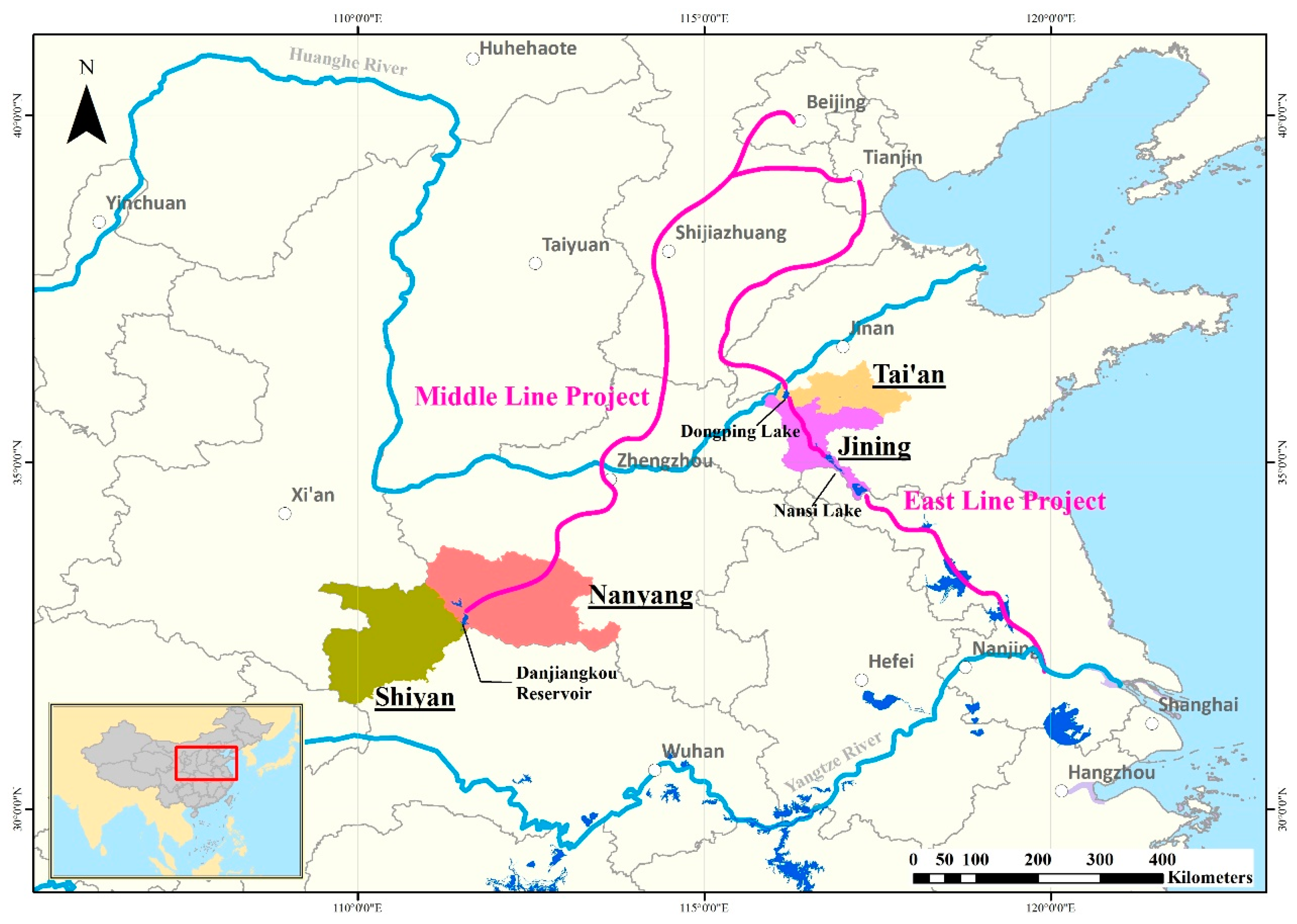
2.1. Study Areas
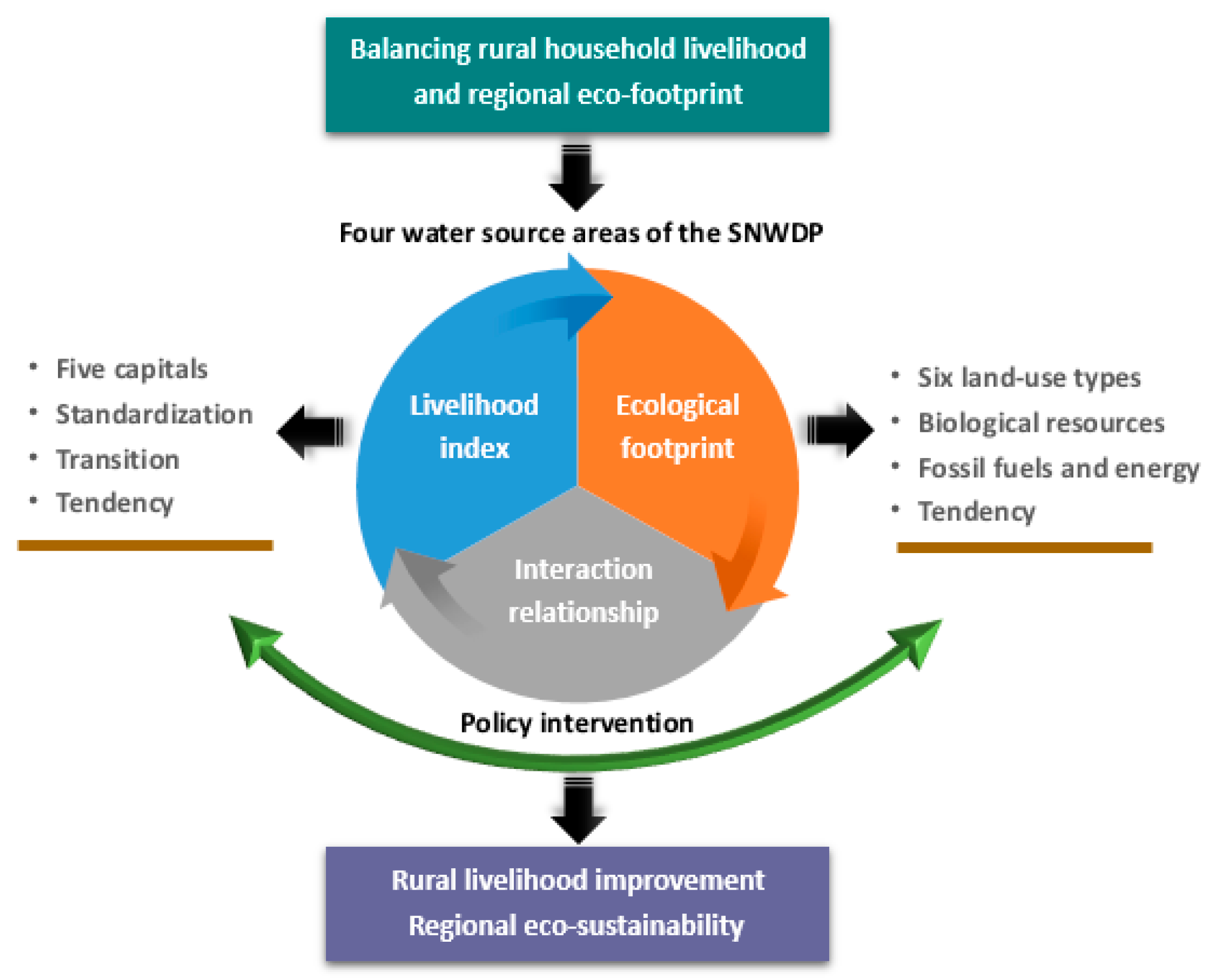
2.2. Research Framework
2.2.1. Selecting the Variables for Analyzing the Change of Rural Livelihood
2.2.2. Calculating the Ecological Footprint in the Four Water Source Areas
2.2.3. Investigating the Relationship between the Livelihood Index and Ecological Footprint
2.3. Data Collection
3. Results
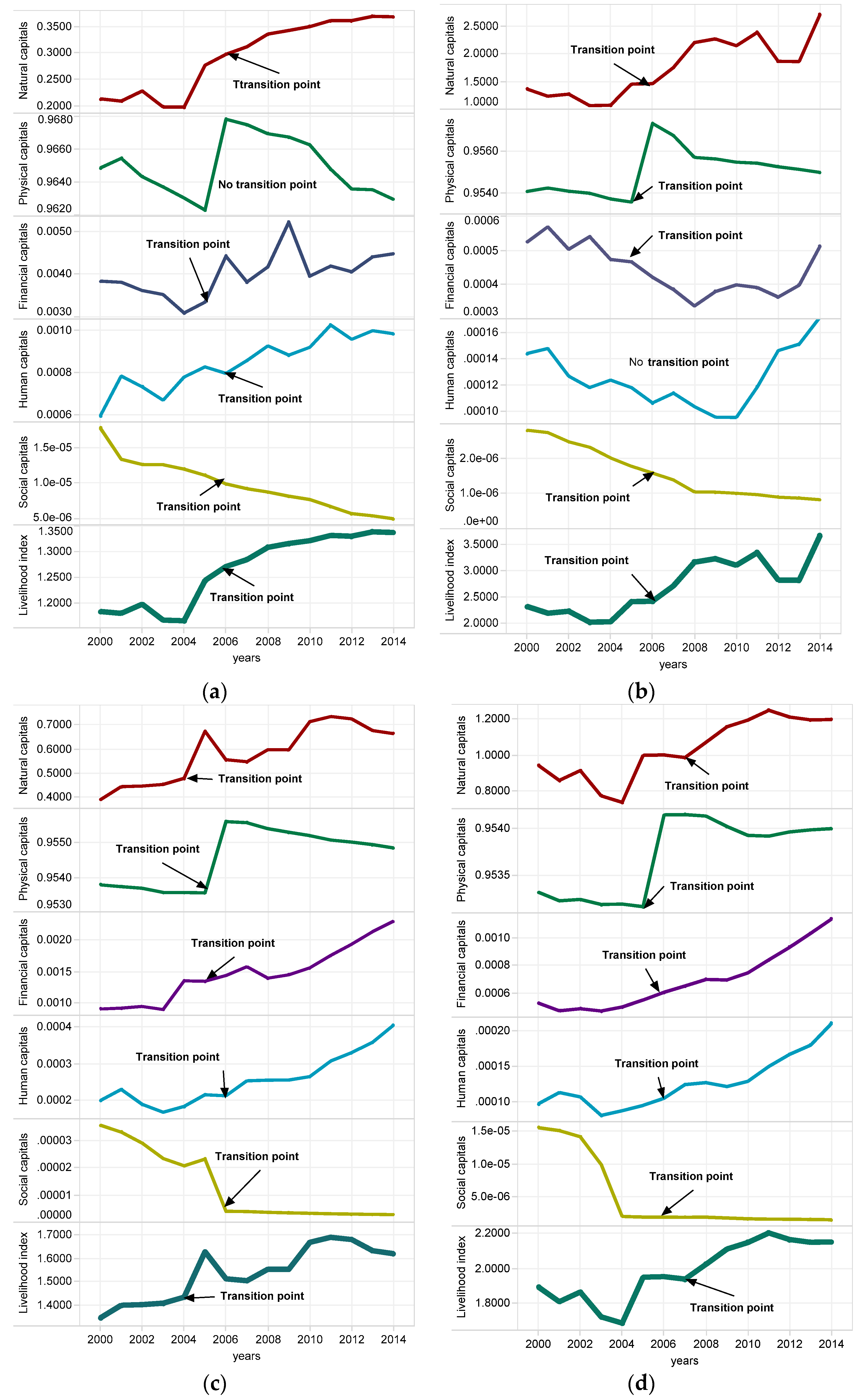
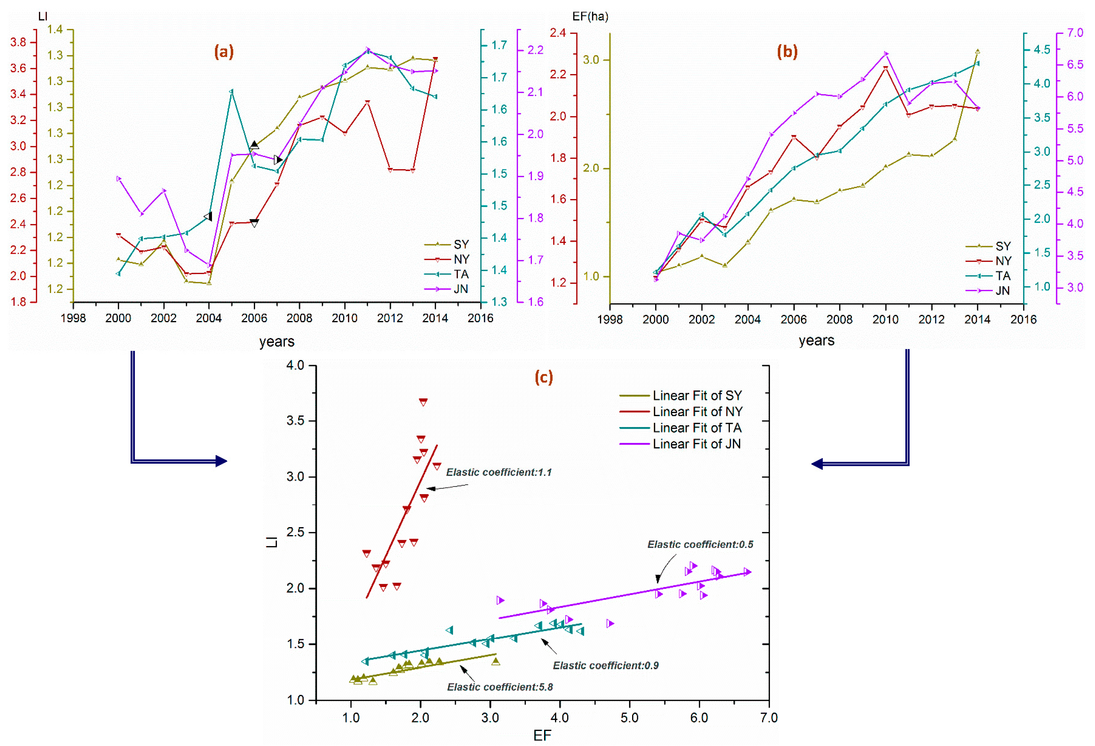
3.1. Change of Rural Livelihood in the Four Water Source Areas
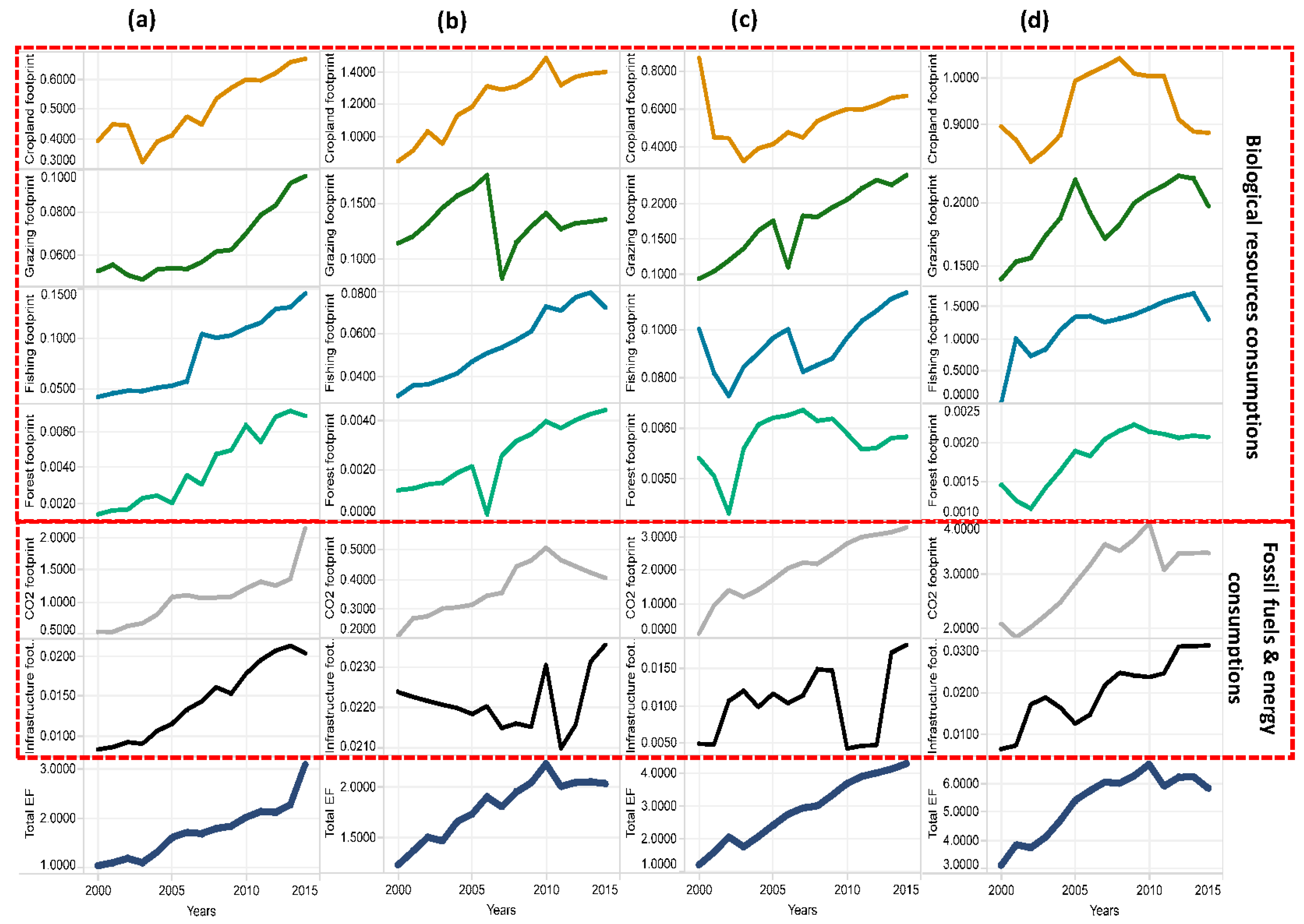
3.2. Change of Ecological Footprints (EF) of Rural Households
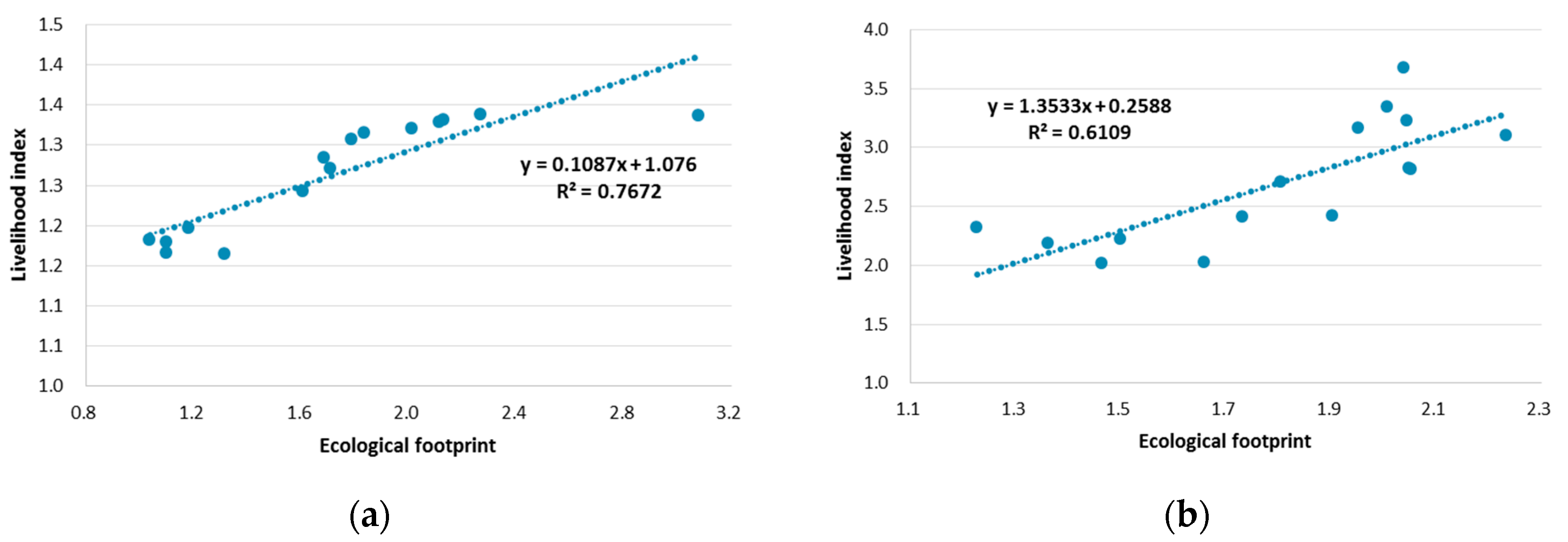
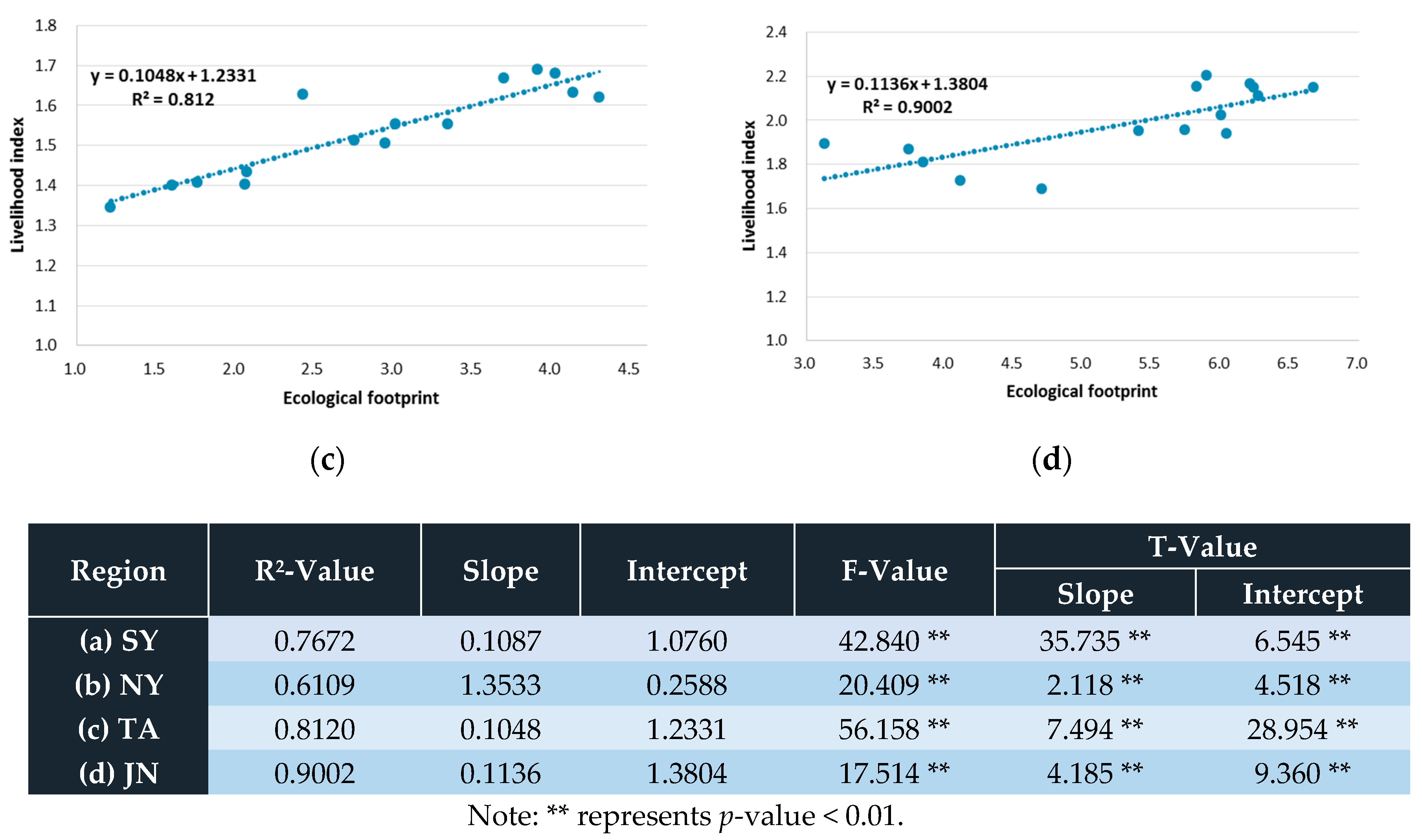
3.3. Relationship between Rural Household Livelihood and Ecological Footprint in These Four Water Source Areas
3.4. Comparisons among These Four Water Source Areas
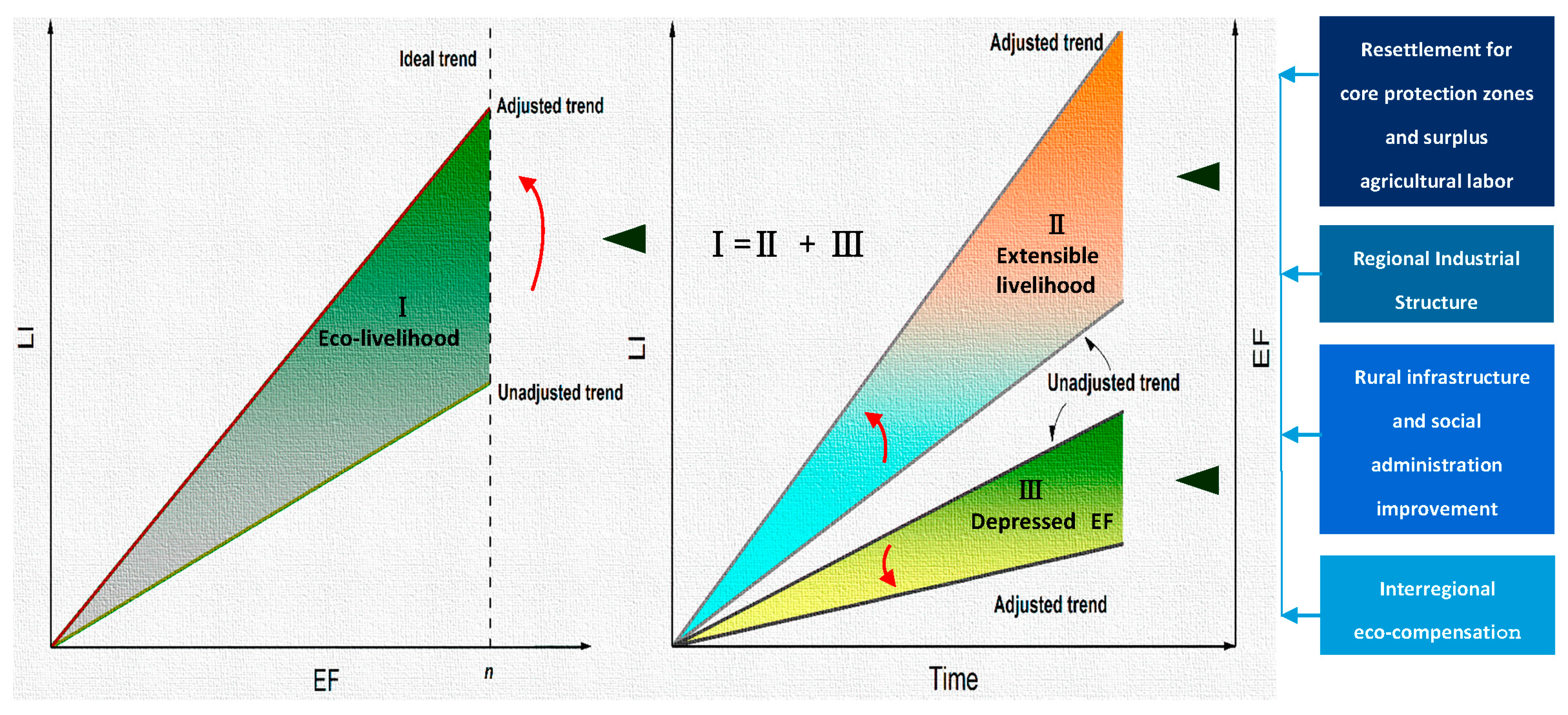
4. Discussions and Conclusions
Acknowledgments
Author Contributions
Conflicts of Interest
References
- World Bank. World Development Indicators; World Bank Publications: Washington, DC, USA, 2016. [Google Scholar]
- Gentle, P.; Maraseni, T.N. Climate change, poverty and livelihoods: Adaptation practices by rural mountain communities in Nepal. Environ. Sci. Policy 2012, 21, 24–34. [Google Scholar]
- Tanner, T.; Lewis, D.; Wrathall, D.; Bronen, R.; Cradock-Henry, N.; Huq, S.; Lawless, C.; Nawrotzki, R.; Prasad, V.; Rahman, Md. A.; et al. Livelihood resilience in the face of climate change. Nat. Clim. Chang. 2015, 5, 23–26. [Google Scholar] [CrossRef]
- Ferrol-Schulte, D.; Wolff, M.; Ferse, S.; Glaser, M. Sustainable Livelihoods Approach in tropical coastal and marine social–ecological systems: A review. Mar. Policy 2013, 42, 253–258. [Google Scholar] [CrossRef]
- Jones, P.G.; Thornton, P.K. Croppers to livestock keepers: Livelihood transitions to 2050 in Africa due to climate change. Environ. Sci. Policy 2009, 12, 427–437. [Google Scholar] [CrossRef]
- Cernea, M.M.; Schmidt-Soltau, K. Poverty Risks and National Parks: Policy Issues in Conservation and Resettlement. World Dev. 2006, 34, 1808–1830. [Google Scholar] [CrossRef]
- Warner, K. Global environmental change and migration: Governance challenges. Glob. Environ. Chang. 2010, 20, 402–413. [Google Scholar] [CrossRef]
- United Nations Educational, Scientific and Cultural Organization. Water for a Sustainable World; United Nations Educational, Scientific and Cultural Organization: Parsi, France, 2015. [Google Scholar]
- Ma, Z.; Kang, S.; Zhang, L.; Tong, L.; Su, X. Analysis of impacts of climate variability and human activity on streamflow for a river basin in arid region of northwest China. J. Hydrol. 2008, 352, 239–249. [Google Scholar] [CrossRef]
- Ellis, F. Rural Livelihoods and Diversity in Developing Countries; Oxford University Press: Oxford, UK, 2000. [Google Scholar]
- Nkemnyi, M.F.; de Haas, A.; Etiendem, N.D.; Ndobegang, F. Making hard choices: Balancing indigenous communities livelihood and Cross River gorilla conservation in the Lebialem–Mone Forest landscape, Cameroon. Environ. Dev. Sustain. 2013, 15, 841–857. [Google Scholar] [CrossRef]
- Singh, N.; Gilman, J. Making Livelihoods Sustainability. Int. Soc. Sci. J. 2000, 17, 123–129. [Google Scholar]
- International Organization for Migration. Outlook on Migration Environment and Climate Change; International Organization for Migration: Geneva, Switzerland, 2015; pp. 21–27. [Google Scholar]
- Gallardo, M.C. Socio-Ecological Inequality and Water Crisis: Views of Indigenous Communities in the Alto Loa Area. Environ. Justice 2016, 9, 9–14. [Google Scholar] [CrossRef]
- Chambers, R.; Conway, G. Sustainable Rural Livelihoods: Practical Concepts for the 21st Century; Institute of Development Studies: Falmer, UK, 1992. [Google Scholar]
- Costanza, R.; de Groot, R.; Sutton, P.; van der Ploeg, S.; Anderson, S.J.; Kubiszewski, I.; Farber, S.; Turner, R.K. Changes in the global value of ecosystem services. Glob. Environ. Chang. 2014, 26, 152–158. [Google Scholar] [CrossRef]
- Leach, M.; Mearns, R.; Scoones, I. Environmental entitlements: Dynamics and institutions in community-based natural resource management. World Dev. 1999, 27, 225–247. [Google Scholar] [CrossRef]
- Daily, G. Nature’s Services: Societal Dependence on Natural Ecosystems; Island Press: Washington, DC, USA, 1997. [Google Scholar]
- Biggs, E.M.; Bruce, E.; Boruff, B.; Duncan, J.M.A.; Horsley, J.; Pauli, N.; McNeill, K.; Neef, A.; Van Ogtrop, F.; Curnow, J.; et al. Sustainable development and the water–energy–food nexus: A perspective on livelihoods. Environ. Sci. Policy 2015, 54, 389–397. [Google Scholar] [CrossRef]
- Scoones, I. Livelihoods perspectives and rural development. J. Peasant Stud. 2009, 36, 171–196. [Google Scholar] [CrossRef]
- Angelsen, A.; Jagger, P.; Babigumira, R.; Belcher, B.; Hogarth, N.J.; Bauch, S.; Börner, J.; Smith-Hall, C.; Wunder, S. Environmental income and rural livelihoods: A global-comparative analysis. World Dev. 2014, 64, S12–S28. [Google Scholar] [CrossRef] [Green Version]
- Sreeja, K.G.; Madhusoodhanan, C.G.; Eldho, T.I. Transforming river basins: Post-livelihood transition agricultural landscapes and implications for natural resource governance. J. Environ. Manag. 2015, 159, 254–263. [Google Scholar] [CrossRef] [PubMed]
- Bebbington, A. Capitals and capabilities: A framework for analyzing peasant viability, rural livelihoods and poverty. World Dev. 1999, 27, 2021–2044. [Google Scholar] [CrossRef]
- Hussein, K. Livelihoods Approaches Compared; Department for International Development: London, UK, 2002.
- Kemkes, R.J. The role of natural capital in sustaining livelihoods in remote mountainous regions: The case of Upper Svaneti, Republic of Georgia. Ecol. Econ. 2015, 117, 22–31. [Google Scholar] [CrossRef]
- Maas, L.T.; Sirojuzilam; Erlina; Badaruddin. The Effect of Social Capital on Governance and Sustainable Livelihood of Coastal City Community Medan. Procedia Soc. Behav. Sci. 2015, 211, 718–722. [Google Scholar] [CrossRef]
- Bhandari, P.B. Rural livelihood change? Household capital, community resources and livelihood transition. J. Rural Stud. 2013, 32, 126–136. [Google Scholar] [CrossRef] [PubMed]
- Morse, S.; Acholo, M.; McNamara, N. Sustainable Livelihood Approach: A Critical Analysis of Theory and Practice; University of Reading: Reading, UK, 2009. [Google Scholar]
- Carr, E.R. Livelihoods as Intimate Government: Reframing the logic of livelihoods for development. Third World Q. 2013, 34, 77–108. [Google Scholar] [CrossRef]
- Sayatham, M.; Suhardiman, D. Hydropower resettlement and livelihood adaptation: The Nam Mang 3 project in Laos. Water Resour. Rural Dev. 2015, 5, 17–30. [Google Scholar] [CrossRef]
- Thapa Karki, S. Do protected areas and conservation incentives contribute to sustainable livelihoods? A case study of Bardia National Park, Nepal. J. Environ. Manag. 2013, 128, 988–999. [Google Scholar] [CrossRef] [PubMed]
- Qing, T. Research Progress and Future Key Trends of Sustainable Livelihoods. Adv. Earth Sci. 2015, 30, 823–833. [Google Scholar]
- Turner, M.D.; Ayantunde, A.A.; Patterson, K.P.; Patterson, E.D., III. Livelihood transitions and the changing nature of farmer-herder conflict in Sahelian West Africa. J. Dev. Stud. 2011, 47, 183–206. [Google Scholar] [CrossRef] [PubMed]
- Bohle, H.-G. Sustainable livelihood security. Evolution and application. In Facing Global Environmental Change; Springer: New York, NY, USA, 2009; pp. 521–528. [Google Scholar]
- Goulden, M.C.; Adger, W.N.; Allison, E.H.; Conway, D. Limits to resilience from livelihood diversification and social capital in lake social–ecological systems. Ann. Assoc. Am. Geogr. 2013, 103, 906–924. [Google Scholar] [CrossRef]
- McLean, J.E. Beyond the pentagon prison of sustainable livelihood approaches and towards livelihood trajectories approaches. Asia Pac. Viewp. 2015, 56, 380–391. [Google Scholar] [CrossRef]
- Reed, M.S.; Podesta, G.; Fazey, I.; Geeson, N.; Hessel, R.; Hubacek, K.; Letson, D.; Nainggolan, D.; Prell, C.; Rickenbach, M.G.; et al. Combining analytical frameworks to assess livelihood vulnerability to climate change and analyse adaptation options. Ecol Econ. 2013, 94, 66–77. [Google Scholar] [CrossRef] [PubMed] [Green Version]
- Singh, P.K.; Hiremath, B.N. Sustainable livelihood security index in a developing country: A tool for development planning. Ecol. Indic. 2010, 10, 442–451. [Google Scholar] [CrossRef]
- Hahn, M.B.; Riederer, A.M.; Foster, S.O. The Livelihood Vulnerability Index: A pragmatic approach to assessing risks from climate variability and change—A case study in Mozambique. Glob. Environ. Chang. 2009, 19, 74–88. [Google Scholar] [CrossRef]
- Donohue, C.; Biggs, E. Monitoring socio-environmental change for sustainable development: Developing a Multidimensional Livelihoods Index (MLI). Appl. Geogr. 2015, 62, 391–403. [Google Scholar] [CrossRef]
- Shah, K.U.; Dulal, H.B.; Johnson, C.; Baptiste, A. Understanding livelihood vulnerability to climate change: Applying the livelihood vulnerability index in Trinidad and Tobago. Geoforum 2013, 47, 125–137. [Google Scholar] [CrossRef]
- Etwire, P.M.; Al-Hassan, R.M.; Kuwornu, J.K.M.; Osei-Owusu, Y. Application of livelihood vulnerability index in assessing vulnerability to climate change and variability in Northern Ghana. J. Environ. Earth Sci. 2013, 3, 157–170. [Google Scholar]
- Wackernagel, M.; Rees, W. Our Ecological Footprint: Reducing Human Impact on the Earth; New Society Publishers: Gabriola Island, BC, Canada, 1998. [Google Scholar]
- Kick, E.L.; McKinney, L.A. Global Context, National Interdependencies, and the Ecological Footprint: A Structural Equation Analysis. Sociol. Perspect. 2014, 57. [Google Scholar] [CrossRef]
- Van den Bergh, J.C.J.M.; Verbruggen, H. Spatial sustainability, trade and indicators: An evaluation of the ‘ecological footprint’. Ecol. Econ. 1999, 29, 61–72. [Google Scholar] [CrossRef]
- Čuček, L.; Klemeš, J.J.; Kravanja, Z. A review of footprint analysis tools for monitoring impacts on sustainability. J. Clean. Prod. 2012, 34, 9–20. [Google Scholar] [CrossRef]
- Li, J.; Liu, Z.; He, C.; Tu, W.; Sun, Z. Are the drylands in northern China sustainable? A perspective from ecological footprint dynamics from 1990 to 2010. Sci. Total Environ. 2016, 553, 223–231. [Google Scholar] [CrossRef] [PubMed]
- Toth, G.; Szigeti, C. The historical ecological footprint: From over-population to over-consumption. Ecol. Indic. 2016, 60, 283–291. [Google Scholar] [CrossRef]
- Aşıcı, A.A.; Acar, S. Does income growth relocate ecological footprint? Ecol. Indic. 2016, 61, 707–714. [Google Scholar] [CrossRef]
- Cobbinah, P.B.; Black, R.; Thwaites, R. Biodiversity conservation and livelihoods in rural Ghana: Impacts and coping strategies. Environ. Dev. 2015, 15, 79–93. [Google Scholar] [CrossRef]
- Gajurel, J.P.; Shrestha, K.K.; Werth, S.; Scheidegger, C. Taxus wallichiana (Himalayan Yew) for the Livelihood of Local People in Some Protected Areas of Nepal. J. Nat. Hist. Mus. 2015, 28, 1–8. [Google Scholar]
- Rantala, S.; Bullock, R.; Mbegu, M.A.; German, L.A. Community-Based Forest Management: What scope for conservation and livelihood co-benefits? Experience from the East Usambara Mountains, Tanzania. J. Sustain. For. 2012, 31, 777–797. [Google Scholar] [CrossRef]
- Bennett, N.J.; Dearden, P. Why local people do not support conservation: Community perceptions of marine protected area livelihood impacts, governance and management in Thailand. Mar. Policy 2014, 44, 107–116. [Google Scholar] [CrossRef]
- Hao, H.; Zhang, J.; Li, X.; Zhang, H.; Zhang, Q. Impact of livelihood diversification of rural households on their ecological footprint in agro-pastoral areas of northern China. J. Arid Land 2015, 7, 653–664. [Google Scholar] [CrossRef]
- Pohlner, H. Institutional change and the political economy of water megaprojects: China’s south-north water transfer. Glob. Environ. Chang. 2016, 38, 205–216. [Google Scholar] [CrossRef]
- Li, G.; Wang, Y. An analysis on environmental protection and compensation policies of South-to-North Water Transfer Project Water Source Area. Stat. Inf. Forum 2015, 30, 92–98. [Google Scholar]
- Wang, L.; Huang, J.; Du, Y. Eco-environmental evaluation of middle route of the South-to-North Water Transfer Project. Resour. Environ. Yangtze Basin 2011, 20, 161–166. [Google Scholar]
- Government of Henan. The Scheme for Dividing the Drinking Water Source Conservation Area in Danjiangkou Reservoir (Henan Province) of South-to-North Water Transfer Project. Available online: http://www.henan.gov.cn/zwgk/system/2015/04/29/010547386.shtml (accessed on 21 June 2015).
- Government of Hubei. The Scheme for Dividing the Drinking Water Source Conservation Area in Danjiangkou Reservoir (Hubei Province) of South-to-North Water Transfer Project. Available online: http://gkml.hubei.gov.cn/auto5472/auto5473/201502/t20150205_616483.html (accessed on 21 June 2015).
- Government of Shandong. The Planning for the Key Ecological Function Areas in Shandong Province. Available online: http://lyc.sdein.gov.cn/swgnbhq/200912/t20091209_208968.html (accessed on 21 June 2015).
- Mensah, E.J. The Sustainable Livelihood Framework: A Reconstruction. Dev. Rev. 2012, 1, 7–24. [Google Scholar]
- Carney, D. Sustainable Livelihoods Approaches: Progress and Possibilities for Change; Department for International Development: London, UK, 2003.
- Bartlett, R.; Bharati, L.; Pant, D.; Hosterman, H.; McCornick, P. Climate Change Impacts and Adaptation in Nepal; IWMI: Durham, NC, USA, 2010. [Google Scholar]
- Sheriff, N.; Little, D.C.; Tantikamton, K. Aquaculture and the poor—Is the culture of high-value fish a viable livelihood option for the poor? Mar. Policy 2008, 32, 1094–1102. [Google Scholar] [CrossRef]
- Government of the People’s Republic of China. The 13th Five-Year Plan for Economic and Social Development of the People’s Republic of China (the 13th Five-Year Plan); Government of the People’s Republic of China: Beijing, China, 2016.
- Heidecke, C. Development and Evaluation of a Regional Water Poverty Index for Benin; International Food Policy Research Institute: Washington, DC, USA, 2006. [Google Scholar]
- Pettitt, A.N. A non-parametric approach to the change-point problem. Appl. Stat. 1979, 28, 126–135. [Google Scholar] [CrossRef]
- Borucke, M.; Moore, D.; Cranston, G.; Gracey, K.; Iha, K.; Larson, J.; Lazarus, E.; Morales, J.C.; Wackernagel, M.; Galli, A. Accounting for demand and supply of the biosphere’s regenerative capacity: The National Footprint Accounts’ underlying methodology and framework. Ecol. Indic. 2013, 24, 518–533. [Google Scholar] [CrossRef]
- Wackernagel, M.; Monfreda, C.; Schulz, N.B.; Erb, K.-H.; Haberl, H.; Krausmann, F. Calculating national and global ecological footprint time series: Resolving conceptual challenges. Land Use Policy 2004, 21, 271–278. [Google Scholar] [CrossRef]
- Dismuke, C.; Lindrooth, R. Ordinary least squares. Methods and Designs for Outcomes Research; ASHP: Bethesda, MD, USA, 2006; p. 93. [Google Scholar]
- Wackernagel, M.; Monfreda, C.; Moran, D.; Wermer, P.; Goldfinger, S.; Deumling, D.; Murray, M. National Footprint and Biocapacity Accounts 2005: The Underlying Calculation Method; Global Footprint Network Oakland: Oakland, CA, USA, 2005. [Google Scholar]
- Lee, Y.-J.; Peng, L.-P. Taiwan’s Ecological Footprint (1994–2011). Sustainability 2014, 6, 6170–6187. [Google Scholar] [CrossRef]
- Huang, B.; Cui, S.; Li, Y. Ecological Footprint Evolution Characteristics and Its Influencing Factors in China from 2000 to 2010. Environ. Sci. 2016, 37, 420–426. [Google Scholar]
- Kincaid, K.B.; Rose, G.A. Why fishers want a closed area in their fishing grounds: Exploring perceptions and attitudes to sustainable fisheries and conservation 10 years post closure in Labrador, Canada. Mar. Policy 2014, 46, 84–90. [Google Scholar] [CrossRef]
- Foale, S.; Manele, B. Social and political barriers to the use of marine protected areas for conservation and fishery management in Melanesia. Asia Pac. Viewp. 2004, 45, 373–386. [Google Scholar] [CrossRef]
- Silva, P. Exploring the Linkages Between Poverty, Marine Protected Area Management, and the Use of Destructive Fishing Gear in Tanzania; World Bank Policy Research Working Paper (3831); World Bank: Washington, DC, USA, 2006. [Google Scholar]
- Allison, E.H.; Ellis, F. The livelihoods approach and management of small-scale fisheries. Mar. Policy 2001, 25, 377–388. [Google Scholar] [CrossRef]
- Zhao, J. Resettlement Management and Practice of the South to North Water Diversion East Project; Shandong University: Jinan, China, 2009. [Google Scholar]
- Zhou, J. The Predicament and the Improvement of Migrant Resettlement Monitoring and Evaluation of South-to-North Water Diversion Project. Jiangsu Soc. Sci. 2011, 6, 61–65. [Google Scholar]
- Bogardi, J.J.; Dudgeon, D.; Lawford, R.; Flinkerbusch, E.; Meyn, A.; Pahl-Wostl, C.; Vielhauer, K.; Vörösmarty, C. Water security for a planet under pressure: interconnected challenges of a changing world call for sustainable solutions. Curr. Opin. Environ. Sustain. 2012, 4, 35–43. [Google Scholar] [CrossRef]
- Lundin, M.; Morrison, G.M. A life cycle assessment based procedure for development of environmental sustainability indicators for urban water systems. Urban Water 2002, 4, 145–152. [Google Scholar] [CrossRef]
- Castellani, V.; Sala, S. Ecological Footprint and Life Cycle Assessment in the sustainability assessment of tourism activities. Ecol. Indic. 2012, 16, 135–147. [Google Scholar] [CrossRef]
- Lo-Iacono-Ferreira, V.G.; Torregrosa-López, J.I.; Capuz-Rizo, S.F. Use of life cycle assessment methodology in the analysis of ecological footprint assessment results to evaluate the environmental performance of universities. J. Clean. Prod. 2016, 133, 43–53. [Google Scholar] [CrossRef]
- Gliessman, S.R. (Ed.) Agroecology: Researching the Ecological Basis for Sustainable Agriculture, Agroecology; Springer: New York, NY, USA, 1990; pp. 3–10. [Google Scholar]
- Garnett, T.; Appleby, M.C.; Balmford, A.; Bateman, I.J.; Benton, T.G.; Bloomer, P.; Burlingame, B.; Dawkins, M.; Dolan, L.; Fraser, D. Sustainable intensification in agriculture: Premises and policies. Science 2013, 341, 33–34. [Google Scholar] [CrossRef] [PubMed] [Green Version]
- Reid, R.S.; Nkedianye, D.; Said, M.Y.; Kaelo, D.; Neselle, M.; Makui, O.; Onetu, L.; Kiruswa, S.; Kamuaro, N.O.; Kristjanson, P. Evolution of models to support community and policy action with science: Balancing pastoral livelihoods and wildlife conservation in savannas of East Africa. Proc. Natl. Acad. Sci. USA 2016, 113, 4579–4584. [Google Scholar] [CrossRef] [PubMed] [Green Version]
- Bremer, L.L.; Farley, K.A.; Lopez-Carr, D.; Romero, J. Conservation and livelihood outcomes of payment for ecosystem services in the Ecuadorian Andes: What is the potential for ‘win–win’? Ecosyst. Serv. 2014, 8, 148–165. [Google Scholar] [CrossRef]


| Captials | Variables | Unit | Change Direction | Justification | Initial Data Source |
|---|---|---|---|---|---|
| Natural capitals (NC) | Agriculture land area (ALA) | ha | + | Land resources are essential for rural livelihoods; the area size of agricultural land can reflect the agricultural land-resource endowment [41]. | Data were collected from the chapters of ‘Agriculture’ in the Shiyan Statistical Yearbooks, Nanyang Statistical Yearbooks, Tai’an Statistical Yearbooks, and Jining Statistical Yearbooks (2000–2015). |
| Industrial waste water discharge (IWWD) | Ton/year | − | Industrial waste water discharge directly reflects the negative impact of industrial activities on the natural environment of water source areas; changes in this variable can be used to explain the effectiveness of water protection, and of the implementation for water quality maintenance policy of water source areas [58,59,61]. | The 15-year data for this variable in each study area were collected from the chapters of ‘Industry’ or ‘Environmental protection’ in the Shiyan Statistical Yearbooks, Nanyang Statistical Yearbooks, Tai’an Statistical Yearbooks, and Jining Statistical Yearbooks. | |
| Precipitation (P) | mm/year | Two-way | Precipitation describes the variation in general characteristics of climate in the water source area [63]. | These data were collected from the chapters of ‘Summary’ and ‘Climate’ in the Statistical Yearbooks (2000–2015) of these four study areas. | |
| Physical capitals (PC) | Total power of agricultural machinery (TPAM) | kWh/year | + | Machinery power reflects the overall quality of agricultural production machinery [64] | The original data for the TPAM were gathered from the chapters of ‘Agriculture’ in the Shiyan Statistical Yearbooks, Nanyang Statistical Yearbooks, Tai’an Statistical Yearbooks, and Jining Statistical Yearbooks (2000–2015). |
| Length of roads (LR) | Km/year | + | Road length is used to reflect the connection of rural residents to the external world [42] | These data were gathered from the chapters of ‘Transportation’ and ‘Infrastructure’ in the Shiyan Statistical Yearbooks, Nanyang Statistical Yearbooks, Tai’an Statistical Yearbooks, and Jining Statistical Yearbooks (2000–2015). | |
| Financial capitals (FC) | Annual net income of rural household (ANIRH) | Yuan/person | + | Net income includes migrant working income, household business income, property income, and transfer income. This variable represents purchasing power, and living standards of rural residents [19]. | These data were collected from the chapters of ‘Rural Household Life’ in the Statistical Yearbooks (2000–2015) of these four study areas. |
| Annual value of rural owned houses (AVROH) | Yuan/Sq.m | + | The value of rural housing changes with the real estate market in the study areas [23,27]. | These data were collected from the chapters of ‘Rural Household Life’ in the Statistical Yearbooks (2000–2015) of these four study areas. | |
| Human Capitals (HC) | Annual consumption of food in rural households(ACFRH) | Yuan/person | Two-way | Food intake reflects the nutritional level of rural residents [19,40]. | These data were collected from the chapters of ‘Rural Household Life’ in the Statistical Yearbooks (2000–2015) of these four study areas. |
| Number of vocational skills schools (NVSS) | Unit/year | + | This variable expresses the involvement of rural residents in vocational skills training and their education level [63]. | The 15-year original data for the NVSS were gathered from the chapters of ‘Education’ in the Shiyan Statistical Yearbooks, Nanyang Statistical Yearbooks, Tai’an Statistical Yearbooks, and Jining Statistical Yearbooks (2000–2015). | |
| Social capitals (SC) | Number of community service facilities (NCSF) | Unit/year | + | This variable reflects the quality of cultural and medical services provided in rural areas. It is an important indicator to explain the comprehensive capacity of social governance in rural grassroots [65]. | These data were collected from the chapters of ‘Community’ and ‘Social Organizations’ in the Statistical Yearbooks (2000–2015) of these four study areas. |
© 2017 by the authors. Licensee MDPI, Basel, Switzerland. This article is an open access article distributed under the terms and conditions of the Creative Commons Attribution (CC BY) license (http://creativecommons.org/licenses/by/4.0/).
Share and Cite
Wang, C.; Shi, G.; Wei, Y.; Western, A.W.; Zheng, H.; Zhao, Y. Balancing Rural Household Livelihood and Regional Ecological Footprint in Water Source Areas of the South-to-North Water Diversion Project. Sustainability 2017, 9, 1393. https://doi.org/10.3390/su9081393
Wang C, Shi G, Wei Y, Western AW, Zheng H, Zhao Y. Balancing Rural Household Livelihood and Regional Ecological Footprint in Water Source Areas of the South-to-North Water Diversion Project. Sustainability. 2017; 9(8):1393. https://doi.org/10.3390/su9081393
Chicago/Turabian StyleWang, Chen, Guoqing Shi, Yongping Wei, Andrew William Western, Hang Zheng, and Yan Zhao. 2017. "Balancing Rural Household Livelihood and Regional Ecological Footprint in Water Source Areas of the South-to-North Water Diversion Project" Sustainability 9, no. 8: 1393. https://doi.org/10.3390/su9081393