An Asymmetric Bimodal Distribution with Application to Quantile Regression

Abstract

In this article, we study an extension of the sinh Cauchy model in order to obtain asymmetric bimodality. The behavior of the distribution may be either unimodal or bimodal. We calculate its cumulative distribution function and use it to carry out quantile regression. We calculate the maximum likelihood estimators and carry out a simulation study. Two applications are analyzed based on real data to illustrate the flexibility of the distribution for modeling unimodal and bimodal data.

1. Introduction

It frequently occurs in real life that we find continuous data that are bimodal; these cannot be modeled by known unimodal distributions. It is therefore of interest to investigate more flexible distributions in modes that will be useful for professionals working in different areas of knowledge.

In unimodal distributions, the flexibility is based on the asymmetry and kurtosis of the data. In this context, Azzalini [1] introduced the skew-normal (SN) distribution, with asymmetry parameter $\lambda$. It has a probability density function (pdf) given by

$$f\left(y;\mu ,\sigma ,\lambda \right)=\frac{2}{\sigma }\varphi \left(\frac{y-\mu }{\sigma }\right)\mathsf{\Phi }\left(\lambda \frac{(y-\mu )}{\sigma }\right),y,\mu ,\lambda \in \mathbb{R},\sigma >0,$$

(1)

where $\varphi$ and $\mathsf{\Phi }$ denote, respectively, the density and cumulative distribution functions of the $N\left(0,1\right)$ distribution. This is denoted as $Y\sim SN\left(\lambda \right)$. SN(0) becomes the standard normal distribution.

Bimodal distributions generated from skew distributions can be found in Ma and Genton [2], Kim [3], Lin et al. [4,5], Elal-Olivero et al. [6], Arnold et al. [7], Arnold et al. [8], and Venegas et al. [9], among others. The importance of studying these distributions is based on the fact that they do not have identifiability problems and can be used as alternative parametric models to replace the use of mixtures of distributions that present estimation problems from either the classical or the Bayesian point of view (see McLachlan and Peel [10]; Marin et al. [11]). One difficulty with these distributions is that in general, there is no closed-form expression for their cumulative distribution function (cdf). This makes it more difficult to generate data from these distributions for simulation studies or to carry out quantile regression. Additionally, many such bimodal distributions have complicated expressions for a general quantile (say, the q-th).

A variety of bimodal data sets and appropriate models have been presented by many authors. For example, Cobb et al. [12] used the quartic exponential density presented by Fisher [13] to model crude birth rates data; Rao et al. [14] used a bimodal distribution to analyze fish length data; Famoye et al. [15] used the beta-normal distribution to analyze egg diameter data; Everitt and Hand [16] discussed some mixture distributions for modeling bimodal data; Chatterjee et al. [17] and Weisberg [18] presented two bimodal data sets on the eruption and interruption times of the Old Faithful geyser; Bansal et al. [19] discussed the bimodality of quantum dot size distribution; Famoye et al. [15] cited a variety of bimodal distributions that arise from different areas of science. On the other hand, the sinh Cauchy (SC) distribution is given by

$$f(z;\Lambda )=\frac{\lambda cosh\left(z\right)}{\sigma \pi (1+{\{\lambda sinh\left(z\right)\}}^2)},$$

where $\Lambda =(\lambda ,\mu ,\sigma )$, $z=\frac{y-\mu }{\sigma }$, $z\in \mathbb{R}$, $\mu \in \mathbb{R}$ is a location parameter, $\sigma >0$ is a scale parameter, and $\lambda >0$ is a symmetric parameter. The SC distribution produces unimodal and bimodal densities. The disadvantage of the SC distribution is that it is symmetric, which limits it to modeling only symmetric bimodal data. The main objective of this article is therefore to study a bimodal skew-symmetric model with closed cdf, in order to apply it to quantile regression. To do this, we used an extension of the SC distribution that we call the gamma–sinh Cauchy (GSC) distribution, which presents flexibility in its modes and also closed-form expression in its cdf. The GSC distribution belongs to the (gamma-G generator) family introduced by Zografos and Balakrishnan [20]. For any baseline cdf $G(y;\Lambda )$, $x\in \mathbb{R}$, they defined the gamma-G generator by the pdf and cdf given by

$$f(y;\varphi ,\Lambda )=\frac{g(y;\Lambda )}{\Gamma \left(\varphi \right)}{\left\{-log\left[1-G(y;\Lambda )\right]\right\}}^{\varphi -1},$$

(2)

and

$$F(y;\varphi ,\Lambda )=\frac{\gamma (-log[1-G(y;\Lambda )],\varphi )}{\Gamma \left(\varphi \right)}=\frac{1}{\Gamma \left(\varphi \right)}{\int }_0^{-log[1-G(y;\Lambda \left)\right]}{u}^{\varphi -1}{e}^{-u}du,$$

(3)

respectively, where $\varphi >0$ is a skewness parameter, $\Lambda$ is a vector of parameters, $g\left(y\right)=\frac{d}{dy}G\left(y\right)$, $\gamma (y,a)={\int }_0^y{t}^{a-1}{e}^{-t}dt$ is the incomplete gamma function, and $\Gamma \left(a\right)=\gamma (+\infty ,a)$ is the usual gamma function. We remark that in the literature, there are many models that can accommodate bimodal distributions. However, in only a few of them do the parameters have an interpretation in terms of measures of central tendency (mean, median, for instance) or a general q-th quantile. As we will show in Section 3, the main advantage of the GSC is that the location parameter represents the respective q-th quantile under a certain restriction over $\varphi$, which is very convenient for the use of this model in a quantile regression framework.

The paper is organized as follows. Section 2 develops the GSC distribution, its basic properties, and quantile regression. In Section 3, we perform a small-scale simulation study of the maximum likelihood (ML) estimators for parameters. Two applications to real data are discussed in Section 4, which illustrate the usefulness of the proposed model. Finally, conclusions are given in Section 5.

2. Gamma–Sinh Cauchy Distribution

The GSC distribution is obtained considering G in (2) as the cdf of the SC distribution. The pdf can be written as

$$f(z;\mathsf{\Theta })=\frac{\lambda cosh\left(z\right)}{\sigma \pi \Gamma \left(\varphi \right)(1+{\{\lambda sinh\left(z\right)\}}^2)}{\left\{-log\left[0.5-\frac{1}{\pi }arctan\left\{\lambda sinh\left(z\right)\right\}\right]\right\}}^{\varphi -1},$$

(4)

where $\mathsf{\Theta }=(\varphi ,\lambda ,\mu ,\sigma )$, and $\varphi >0$ is an asymmetric parameter. We denoted this by $Z\sim GSC(\varphi ,\lambda ,\mu ,\sigma )$.

The cdf is given by

$$F(z;\varphi ,\lambda ,\mu ,\sigma )=\frac{1}{\Gamma \left(\varphi \right)}\gamma \left(-log\left[0.5-\frac{1}{\pi }arctan\{\lambda sinh\left(z\right)\}\right],\varphi \right).$$

(5)

Particular cases:

• $\varphi =1$ SC distribution,
• $\varphi =1$, $\lambda =1$ hyperbolic secant distribution (Talacko [21]).

The following proposition states conditions for the symmetry of the GSC distribution.

Proposition 1.

The density of the $GSC(\varphi ,\lambda ,\mu ,\sigma )$ model is symmetric if and only if $\varphi =1$.

Proof. 

Without loss of generality, we consider $\mu =0$ and $\sigma =1$. For $\varphi =1$, the density of the model is

$$f(y;1,\lambda ,0,1)=\frac{\lambda cosh\left(y\right)}{\sigma \pi \Gamma \left(\varphi \right)(1+{\{\lambda sinh\left(y\right)\}}^2)}.$$

This function is clearly even because $cosh\left(y\right)$ and $sinh{\left(y\right)}^2$ are even. To prove the reciprocal, we will argue by contradiction. Let ${\varphi }_0\ne 1$ such that the density is symmetric, i.e. $f(y;{\varphi }_0,\lambda ,0,1)=f(-y;{\varphi }_0,\lambda ,0,1)$, $\forall y\in \mathbb{R},\forall \lambda >0$. This implies that

$${\left(\frac{log\left[\frac{1}{2}+\frac{1}{\pi }arctan\left\{\lambda sinh\left(y\right)\right\}\right]}{log\left[\frac{1}{2}-\frac{1}{\pi }arctan\left\{\lambda sinh\left(y\right)\right\}\right]}\right)}^{{\varphi }_0-1}=1.$$

From the latter equality, and jointly with the fact that the logarithmic function is injective, we find that $arctan(\lambda sinh(y\left)\right)=0$, $\forall y\in \mathbb{R}$, which implies that $\lambda =0$, producing a contradiction. □

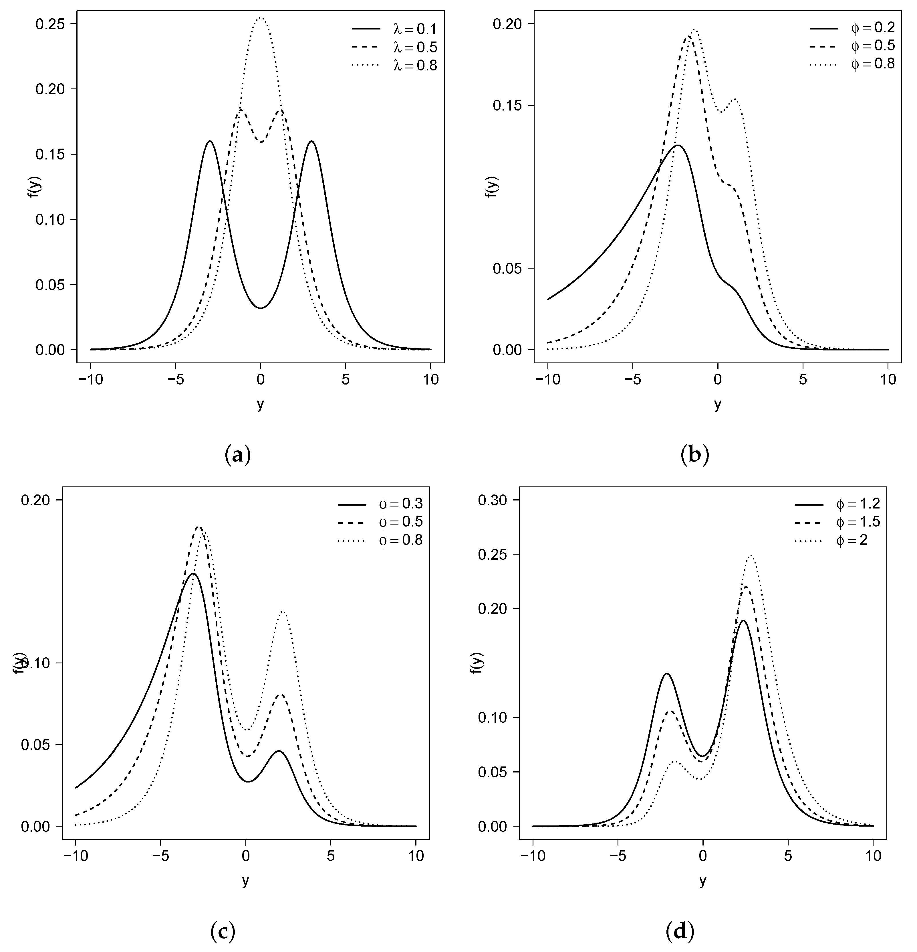
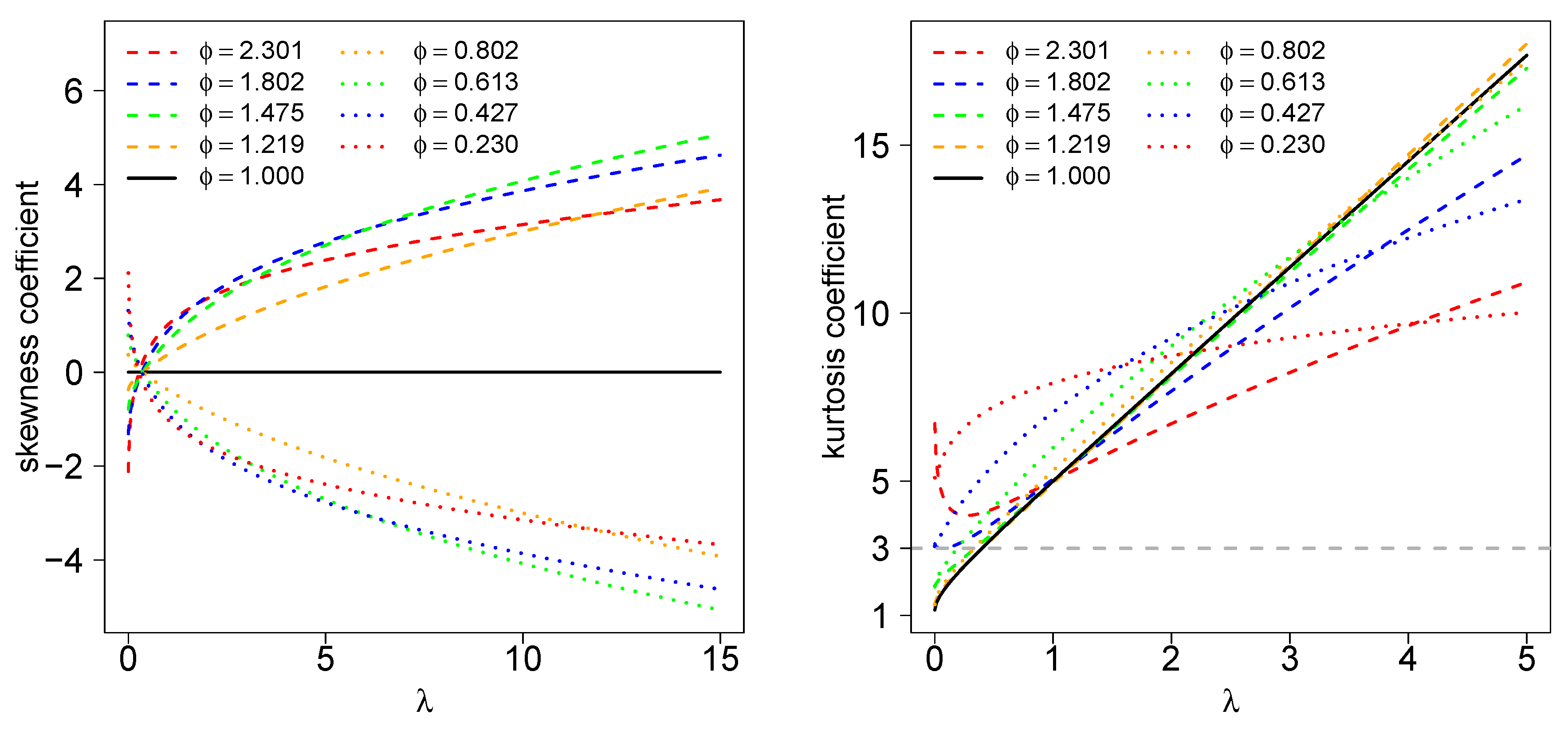
The unimodal and bimodal regions for $GSC(\varphi ,\lambda ,\mu ,\sigma )$ are illustrated in Figure 1. We can see that for all $\varphi$, there is $\lambda$ such that $GSC$ is bimodal. Figure 2 shows the density function for some values of the parameters $\varphi$ and $\lambda$, considering the location and scale parameters fixed at 0 and 1, respectively. The distribution assumes symmetric unimodal and bimodal shapes and asymmetric unimodal and bimodal shapes. Figure 3 shows the skewness and kurtosis coefficients for the GSC model under different values of $\lambda$ and $\varphi$ (such coefficients do not depend on $\mu$ and $\sigma$). As illustrated previously, the model can assume positive and negative values for the skewness coefficient and can also accommodate kurtosis coefficients lower than, equal to, and greater than the normal model (<3, =3 and >3, respectively).

The GSC Model for Quantile Regression

From Equation (5), it follows that the cdf of the GSC distribution evaluated in $\mu$ is given by

$$P(Y\le \mu ;\varphi ,\lambda ,\mu ,\sigma )=F(\mu ;\varphi ,\lambda ,\mu ,\sigma )=\frac{\gamma (log(2),\varphi )}{\Gamma \left(\varphi \right)}=G\left(log\left(2\right),\varphi \right),$$

(6)

where $G(y,a)=\gamma (y,a)/\Gamma \left(a\right)$ corresponds to the cdf of the gamma distribution with shape and scale parameters a and 1, respectively. Note that $G\left(log\left(2\right),\varphi \right)$ depends only on $\varphi$ (and not on $\sigma$ or $\lambda$). As $G(log(2),\varphi )$ is an increasing function in terms of $\varphi$ and $G(·,\varphi )\in (0,1)$, the equation $G(log(2),\varphi )=q$ has an unique solution for $q\in (0,1)$, which can also be written as

$$\frac{1}{\Gamma \left(\varphi \right)}{\int }_0^{log\left(2\right)}{u}^{\varphi -1}{e}^{-u}du=q.$$

(7)

Equation (7) can be solved numerically. For instance, in R the uniroot function can be used.

Table 1. Some values for $\varphi \left(q\right)$ in terms of q.

q	$0.1$	$0.2$	$0.3$	$0.4$	$0.5$	$0.6$	$0.7$	$0.8$	$0.9$
$\mathit{\varphi }\left(\mathit{q}\right)$	2.301	1.802	1.475	1.219	1.000	0.802	0.613	0.427	0.230

shows some values for $\varphi \left(q\right)$ with different values for q.

For this reason, for a fixed q, if we take $\varphi =\varphi \left(q\right)$ satisfying (7), by (6) the parameter $\mu$ directly represents the q-th quantile, allowing regression to be performed conveniently even though $\mu$. Under this setting, a set of available p-covariates, say ${\mathit{x}}_i^{\top }=(x_{i1},\dots ,x_{ip})$, for $i=1,\dots ,n$, can be introduced as follows:

$${\mu }_i={\mathit{x}}_i^{\top }\mathit{\beta },i=1,\dots ,n.$$

This is a convenient property of the GSC distribution because it provides a simple way to performing quantile regression in a model that can be unimodal or bimodal, depending only on parameter $\lambda$ (because $\varphi =\varphi \left(q\right)$ is considered as fixed in this setting).

As far as we know, there is no model in the literature that is parameterized conveniently in terms of the q-th quantile and can also be unimodal or bimodal. Figure 1 shows that for any $\varphi =\varphi \left(q\right)$ fixed in the GSC, there is an interval ${\Lambda }_{\varphi \left(q\right)}^{\left(1\right)}$ for $\lambda$ where the distribution is unimodal and an interval ${\Lambda }_{\varphi \left(q\right)}^{\left(2\right)}$ where the distribution is bimodal.

3. ML Estimation for the GSC Distribution

3.1. ML Estimation

Consider $y_1,y_2,\cdots ,y_n$ as a size n random sample from the pdf $GSC(\varphi ,\lambda ,\mu ,\sigma )$. Hence, the log-likelihood function is given by

$$\begin{array}{cc}\hfill l(\varphi ,\lambda ,\mu ,\sigma )& =nlog\left(\lambda \right)+\sum _{i=1}^{n}log\{cosh\left(z_i\right)\}-\sum _{i=1}^{n}log\left\{1+{\lambda }^2{sinh}^2\left(z_i\right)\right\}\hfill \\ & +(\varphi -1)\sum _{i=1}^{n}log\left\{-log\left[\frac{1}{2}-\frac{1}{\pi }arctan\{\lambda sinh\left(z_i\right)\}\right]\right\}\hfill \\ & -nlog\left(\sigma \right)-nlog\left(\pi \right)-nlog(\Gamma (\varphi \left)\right),\hfill \end{array}$$

(8)

where $z_i=\frac{y_i-\mu }{\sigma }$. To compute the ML estimation for $\mathsf{\Theta }=(\varphi ,\lambda ,\mu ,\sigma )$, (8) must be maximized. That is, we have to solve the following system of equations: $\frac{\delta l}{\delta \varphi }$, $\frac{\delta l}{\delta \lambda }$, $\frac{\delta l}{\delta \mu }$, and $\frac{\delta l}{\delta \sigma }$. More precisely, we have to solve

$$\begin{array}{ccc}\hfill \sum _{i=1}^{n}log(-log\left(t_i\right))-n\mathsf{\Psi }\left(\varphi \right)& =& 0,\hfill \\ \hfill \sum _{i=1}^n\frac{2\lambda {sinh}^2\left(z_i\right)}{1+{\lambda }^2{sinh}^2\left(z_i\right)}+(\varphi -1)\sum _{i=1}^n\frac{sinh\left(z_i\right)}{\pi t_i(1+{\lambda }^2{sinh}^2\left(z_i\right))log\left(t_i\right)}& =& \frac{n}{\lambda },\hfill \\ \hfill \sum _{i=1}^n\frac{{\lambda }^{2}sinh\left(2z_i\right)}{1+{\lambda }^2{sinh}^2\left(z_i\right)}+\frac{\lambda (\varphi -1)}{\pi }\sum _{i=1}^n\frac{cosh\left(z_i\right)}{t_i(1+{\lambda }^2{sinh}^2\left(z_i\right))log\left(t_i\right)}& =& \sum _{i=1}^{n}tanh\left(z_i\right),\hfill \\ \hfill \sum _{i=1}^n\frac{{\lambda }^2{z}_{i}sinh\left(2z_i\right)}{1+{\lambda }^2{sinh}^2\left(z_i\right)}+\frac{\lambda (\varphi -1)}{\pi }\sum _{i=1}^n\frac{z_{i}cosh\left(z_i\right)}{t_i(1+{\lambda }^2{sinh}^2\left(z_i\right))log\left(t_i\right)}-n& =& \sum _{i=1}^n{z}_{i}tanh\left(z_i\right),\hfill \end{array}$$

where $t_i=\frac{1}{2}-\frac{1}{\pi }arctan\{\lambda sinh\left(z_i\right)\}$, and $\mathsf{\Psi }(·)$ is the digamma function. The system of equations given above can be solved using numerical procedures such as the Newton–Raphson procedure. An alternative is to use the NumDeriv routine with the R software (R Core Team [22]).

3.2. Simulation Study

In this Section, we present a brief simulation study to assess the performance of MLE in the GSC model. To draw values from the model, we used the inversion method. If $U\sim U(0,1)$, then

$$Z=\mu +\sigma {sinh}^{-1}\left({\lambda }^{-1}tan\left[\pi /2-\pi exp\left(-G^{-1}\left(U;\varphi \right)\right)\right]\right)\sim GSC(\varphi ,\lambda ,\mu ,\sigma ),$$

where $G^{-1}(·;\varphi )$ is the inverse of the cdf of the gamma distribution with shape and rate parameters equal to $\varphi$ and 1, respectively. In all scenarios, we considered $\mu =0$ and $\sigma =1$, three values for $\varphi$—$0.75,1$, and $1.5$—and three values for $\lambda$—$0.5,1$, and 2. We also considered three sample sizes: 100, 200, and 500. For each combination of the parameters, we drew 1,000 samples and computed the ML estimates.

Table 2. Simulation study for the GSC $(\varphi ,\lambda ,\mu =0,\sigma =1)$ model.

			$\mathit{n}=100$			$\mathit{n}=200$			$\mathit{n}=500$
$\mathit{\varphi }$	$\mathit{\lambda }$	parameter	bias	RMSE	CP	bias	RMSE	CP	bias	RMSE	CP
0.75	0.5	$\mu$	−0.094	0.663	0.846	−0.055	0.578	0.900	−0.014	0.457	0.932
		$\sigma$	−0.037	0.392	0.880	−0.014	0.337	0.904	−0.006	0.268	0.933
		$\lambda$	−0.031	0.372	0.869	−0.013	0.317	0.905	−0.006	0.252	0.930
		$\varphi$	0.044	0.411	0.867	0.023	0.349	0.907	0.006	0.272	0.934
	1.0	$\mu$	−0.015	0.607	0.831	0.021	0.532	0.880	0.016	0.428	0.925
		$\sigma$	−0.035	0.460	0.848	−0.024	0.396	0.886	−0.009	0.320	0.927
		$\lambda$	−0.004	0.544	0.831	−0.010	0.459	0.889	−0.003	0.365	0.927
		$\varphi$	0.018	0.424	0.843	−0.004	0.363	0.890	−0.006	0.290	0.926
	2.0	$\mu$	0.011	0.361	0.934	0.004	0.298	0.944	0.001	0.233	0.944
		$\sigma$	−0.011	0.504	0.911	−0.007	0.419	0.932	−0.003	0.333	0.945
		$\lambda$	0.055	0.789	0.928	0.017	0.650	0.939	0.010	0.513	0.945
		$\varphi$	−0.007	0.337	0.940	−0.003	0.279	0.949	−0.001	0.220	0.947
1.0	0.5	$\mu$	−0.060	0.666	0.846	−0.036	0.580	0.899	−0.012	0.460	0.933
		$\sigma$	−0.044	0.373	0.877	−0.022	0.318	0.915	−0.009	0.253	0.933
		$\lambda$	−0.033	0.366	0.867	−0.018	0.308	0.913	−0.007	0.245	0.936
		$\varphi$	0.045	0.458	0.874	0.023	0.388	0.909	0.007	0.304	0.938
	1.0	$\mu$	−0.052	0.622	0.816	−0.024	0.543	0.881	−0.002	0.428	0.940
		$\sigma$	−0.040	0.431	0.832	−0.024	0.367	0.887	−0.006	0.293	0.936
		$\lambda$	−0.017	0.535	0.811	−0.015	0.448	0.875	0.000	0.354	0.934
		$\varphi$	0.060	0.493	0.842	0.027	0.417	0.890	0.005	0.324	0.946
	2.0	$\mu$	−0.001	0.357	0.937	0.000	0.291	0.946	−0.001	0.229	0.951
		$\sigma$	−0.014	0.494	0.896	−0.006	0.413	0.929	0.000	0.328	0.942
		$\lambda$	0.033	0.795	0.916	0.017	0.658	0.937	0.011	0.521	0.944
		$\varphi$	0.007	0.372	0.942	0.002	0.303	0.947	0.002	0.238	0.949
1.5	0.5	$\mu$	0.015	0.683	0.850	0.014	0.597	0.894	0.008	0.480	0.925
		$\sigma$	−0.045	0.354	0.890	−0.021	0.300	0.926	−0.009	0.239	0.935
		$\lambda$	−0.022	0.366	0.877	−0.014	0.308	0.916	−0.006	0.245	0.937
		$\varphi$	0.026	0.533	0.876	0.008	0.455	0.906	0.002	0.364	0.930
	1.0	$\mu$	−0.134	0.688	0.835	−0.138	0.612	0.856	−0.076	0.492	0.904
		$\sigma$	-0.038	0.413	0.836	−0.025	0.347	0.856	−0.011	0.275	0.896
		$\lambda$	0.091	0.581	0.840	−0.001	0.459	0.860	−0.010	0.360	0.896
		$\varphi$	0.211	0.681	0.886	0.166	0.579	0.880	0.076	0.446	0.912
	2.0	$\mu$	−0.029	0.383	0.933	−0.009	0.309	0.945	−0.004	0.241	0.948
		$\sigma$	−0.014	0.472	0.895	−0.007	0.395	0.927	−0.003	0.313	0.942
		$\lambda$	0.065	0.784	0.932	0.023	0.646	0.942	0.010	0.510	0.952
		$\varphi$	0.070	0.484	0.948	0.023	0.379	0.954	0.009	0.294	0.950

summarizes the results considering the average of the bias (bias), the root of the estimated mean squared error (RMSE), and the 95% coverage probability (CP). Note that in all cases, the bias and RMSE decreased when the sample size was increased, suggesting that the estimators are consistent. Finally, we also remark that the coverage probability converged to the nominal values used for the construction of the confidence intervals when the sample size was increased, suggesting that the normality for the ML estimates is reasonable in sample sizes.

4. Applications

In this section, we carry out two applications to real data, the first using the GSC model without covariates and the second applying quantile regression to uni- and bimodal data.

4.1. Application 1: Without Covariates

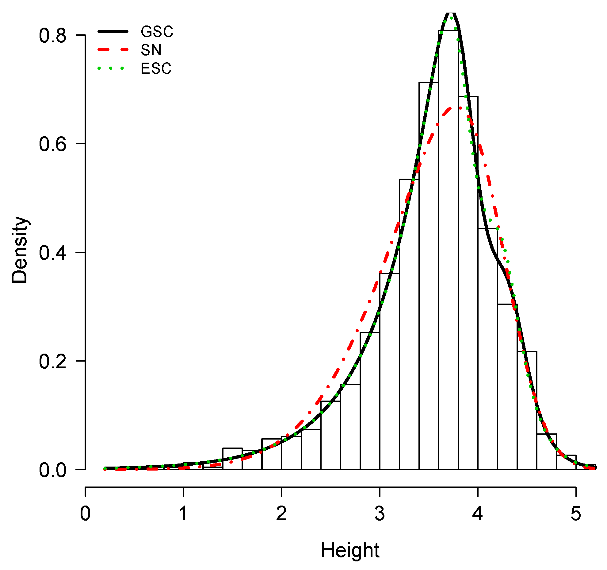
The first application reported is for the data set consisting of 1150 heights measured at 1 micron intervals along the drum of a roller (i.e., parallel to the axis of the roller). This was part of an extensive study of roller surface roughness. It is available for downloading at http://lib.stat,emu.edu/jasadata/laslett.

Table 3. Descriptive statistics for the data set.

n	$\overline{\mathit{y}}$	${\mathit{s}}^2$	${\mathit{b}}_1$	${\mathit{b}}_2$
1150	3.535	0.422	−0.986	4.855

presents summary statistics for the data set where $b_1$ and $b_2$ correspond to the sample asymmetry and kurtosis coefficients, respectively.

We fitted this using the SN model, the exponentiated sinh Cauchy (ESC) model (see Cooray [23]), and the GSC model. A summary of these fits is presented in

Table 4. Maximum likelihood (ML) estimates for the GSC, exponentiated sinh Cauchy (ECG), and skew-normal (SN) models for the roller data set.

Parameter	GSC	ECG	SN
$\mu$	4.1115 (0.0388)	4.0460 (0.0482)	4.2475 (0.0276)
$\sigma$	0.2053 (0.0172)	0.1903 (0.0205)	0.9644 (0.0286)
$\lambda$	0.5353 (0.0682)	0.5535 (0.0860)	−2.7578 (0.2426)
$\varphi$	0.3621 (0.0373)	0.3322 (0.0445)	−
log-likelihood	−1053.8	−1056.0	−1071.3
AIC	2115.7	2119.9	2148.7

. Based on the AIC criteria, the GSC provided the best fit for the height data set. Figure 4 shows plots of the density functions for the fitted models using the MLEs for SN, ECG and GSC distributions.

4.2. Data Set 2: Quantile Regression to Bimodal Data

The second application we consider is the Australian data set available in the sn package in R. This data set is related to 102 male and 100 female athletes collected at the Australian Institute of Sport. The linear model considered is

$$\begin{array}{c}\hfill {\mathtt{Bfat}}_i={\beta }_0\left(q\right)+{\beta }_1\left(q\right){\mathtt{bmi}}_i+{\beta }_2\left(q\right){\mathtt{lbm}}_i+{ϵ}_i\left(q\right),i=1,\dots ,202,\end{array}$$

(9)

where ${\mathtt{Bfat}}_i$ is the body fat percentage for the i-th athlete and ${\mathtt{bmi}}_i$ and ${\mathtt{lbm}}_i$ are the covariates body mass index and lean body mass for the i-th athlete, respectively. In addition, ${ϵ}_i\left(q\right)\sim GSC(0,\sigma ,\lambda ,\varphi \left(q\right))$, $\varphi \left(q\right)$ satisfies Equation (7), and $q\in (0,1)$ is the fixed quantile that is being modeled. This data set was also analyzed in Martínez-Flórez et al. [24] using a bimodal regression model. However, the authors modeled the mean of the distribution. In our approach, we model the $0.1,0.25,0.5,0.75$, and $0.9$ percentiles of the distribution, which provides a more informative scenario to explain body fat in terms of the body mass index and lean body mass. Our approach is compared with the skewed Laplace (SKL) and skewed Student-t (SKT) models discussed in Galarza et al. [25], where the authors proposed a flexible model in a quantile regression model context.

Table 5. AIC and p-value for K–S test in the ais data set for the GSC, skewed Laplace (SKL), and skewed Student-t (SKT) models and different quantiles.

	AIC			p-value for K–S test
q	GSC	SKL	SKT	GSC	SKL	SKT
$0.10$	1156.54	1194.28	1166.74	0.79	0.06	0.02
$0.25$	1160.72	1172.70	1153.15	0.65	0.71	0.96
$0.50$	1162.74	1182.66	1161.80	0.32	0.13	0.31
$0.75$	1159.50	1221.65	1200.87	0.87	<0.001	0.02
$0.90$	1211.71	1280.45	1253.48	0.02	<0.001	<0.001

shows the AIC for those models considering different quantiles. We also present the p-value for the Kolmogorov–Smirnov (K–S) test of the hypothesis that the respective quantile residuals came from the standard normal distribution. P-values greater than 5% suggest that with this significance level, the standard normal assumption is reasonable for those residuals, in which case the model would be appropriate for this data set. Note that based on the AIC criteria, the GSC presents a better fit for this data set, except for the median regression ($q=0.5$). On the other hand, based on the p-value for the K–S test applied to the quantile residuals, we conclude that GSC, SKL, and SKT are appropriate models for $q=0.25$ and $q=0.5$ (the GSC and SKT provide a better fit based on the AIC criteria). However, for $q=0.1$ and $0.75$, GSC provides the better fit because the p-values are (significantly) greater than 0.05. Finally, for $q=0.9$ no model seems appropriate, but based on the p-values, the GSC provides a better fit than SKL and SKT distributions.

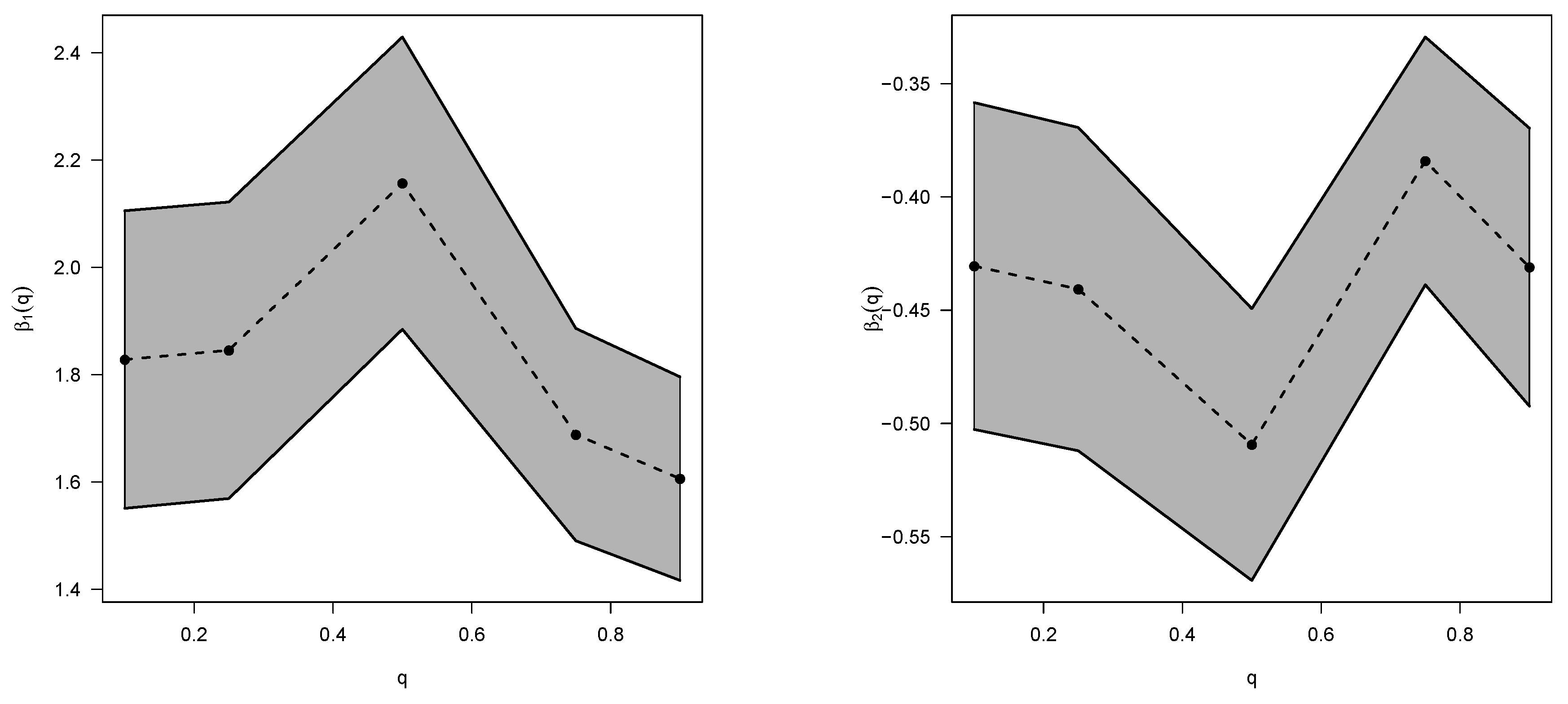
Figure 5 shows the regression coefficients for the quantile regression presented in Equation (9) and their respective 95% confidence intervals. Note that body mass index and lean body mass are significant in explaining all the quantiles modeled.

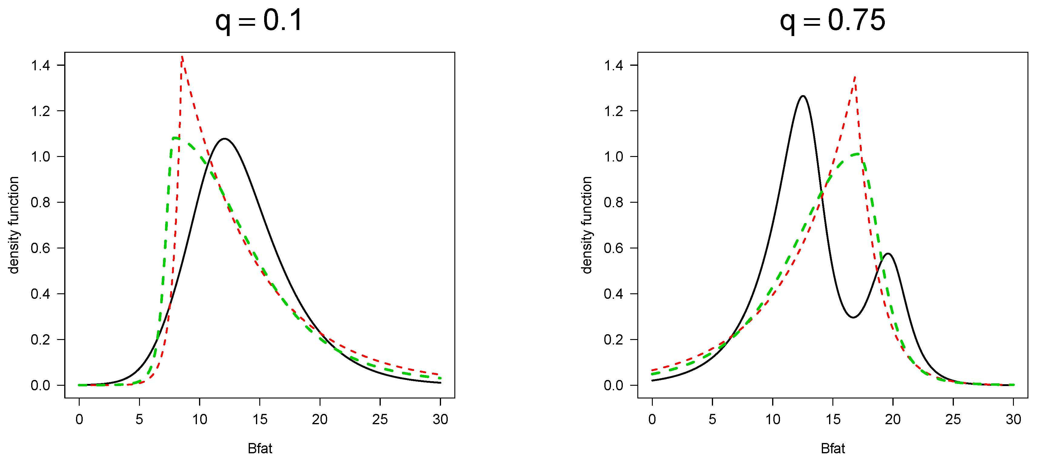
Figure 6 shows the profile density for the q-th quantile of body fat percentage for $q=0.1$ and $q=0.75$. Note that the distribution of the $0.1$ quantile is unimodal, and the distribution of the $0.9$ quantile is bimodal.

5. Final Comments

This paper proposes the GSC distribution, which is flexible in its modes and contains the SC distribution as a special case. We implemented ML estimation in a quantile regression, obtaining significant results. In the applications to real data it performs very well, better than potential rival models. Some further characteristics of the GSC distribution are:

• The GSC distribution contains the SC and hyperbolic secant models as special cases.
• The GSC distribution presents great flexibility in its modes, as can be observed in Figure 1.
• The proposed model has a closed-form expression for its cdf.
• In the two applications, we show that the GSC model fits better than the other models.

References

- Azzalini, A. A class of distributions which includes the normal ones. Scand. J. Stat. 1985, 12, 171–178. [Google Scholar]
- Ma, Y.; Genton, M.G. Flexible class of skew-symmetric distributions. Scand. J. Stat. 2004, 31, 459–468. [Google Scholar] [CrossRef]
- Kim, H.J. On a class of two-piece skew-normal distributions. Statistics 2005, 39, 537–553. [Google Scholar] [CrossRef]
- Lin, T.I.; Lee, J.C.; Hsieh, W.J. Robust mixture models using the skew-t distribution. Stat. Comput. 2007, 17, 81–92. [Google Scholar] [CrossRef]
- Lin, T.I.; Lee, J.C.; Yen, S.Y. Finite mixture modeling using the skew-normal distribution. Stat. Sin. 2007, 17, 909–927. [Google Scholar]
- Elal-Olivero, D.; Gómez, H.W.; Quintana, F.A. Bayesian Modeling using a class of Bimodal skew-Elliptical distributions. J. Stat. Plan. Infer. 2009, 139, 1484–1492. [Google Scholar] [CrossRef]
- Arnold, B.C.; Gómez, H.W.; Salinas, H.S. On multiple constraint skewed models. Statistics 2009, 43, 279–293. [Google Scholar] [CrossRef]
- Arnold, B.C.; Gómez, H.W.; Salinas, H.S. A doubly skewed normal distribution. Statistics 2015, 49, 842–858. [Google Scholar] [CrossRef]
- Venegas, O.; Salinas, H.S.; Gallardo, D.I.; Bolfarine, H.; Gómez, H.W. Bimodality based on the generalized skew-normal distribution. J. Stat. Comput. Simul. 2018, 88, 156–181. [Google Scholar] [CrossRef]
- McLachlan, G.J.; Peel, D. Finite Mixture Models; Wiley Interscience: New York, NY, USA, 2000. [Google Scholar]
- Marin, J.M.; Mengersen, K.; Robert, C. Bayesian modeling and inference on mixtures of distributions. Handbook Stat. 2005, 25, 459–503. [Google Scholar]
- Cobb, L.; Koppstein, P.; Chen, N.H. Estimation and moment recursion relations for multimodal distributions of the exponential families. J. Arner. Stat. Assoc. 1983, 78, 124–130. [Google Scholar] [CrossRef]
- Fisher, R.A. On the Mathematical Foundations of Theoretical Statistics. Philos. Trans. R. Soc. London Ser. A 1922, 222, 309–368. [Google Scholar] [CrossRef]
- Rao, K.S.; Narayana, J.L.; Sastry, V.P. A bimodal distribution. Bull. Calcutta Math. Soc. 1988, 80, 238–240. [Google Scholar]
- Famoye, F.; Lee, C.; Eugene, N. Beta-normal distribution: Bimodality properties and application. J. Modern Appl. Stat. Method 2004, 3, 85–103. [Google Scholar] [CrossRef]
- Everitt, B.S.; Hand, D.J. Finite Mixture Distributions; Chapman & Hall: London, UK, 1981. [Google Scholar]
- Chatterjee, S.; Handcock, M.S.; Simonoff, J.S. A Casebook for a First Course in Statistics and Data Analysis; John Wiley & Sons: New York, NY, USA, 1995. [Google Scholar]
- Weisberg, S. Applied Linear Regression; John Wiley & Sons: New York, NY, USA, 2005. [Google Scholar]
- Bansal, B.; Gokhale, M.R.; Bhattacharya, A.; Arora, B.M. InAs/InP quantum dots with bimodal size distribution: Two evolution pathways. J. Appl. Phys. 2007, 101, 1–6. [Google Scholar] [CrossRef]
- Zografos, K.; Balakrishnan, N. On families of beta- and generalized gamma-generated distributions and associated inference. Stat. Methodol. 2009, 6, 344–362. [Google Scholar] [CrossRef]
- Talacko, J. Perks’ distributions and their role in the theory of Wiener’s stochastic variables. Trabajos de Estadistica 1956, 7, 159–174. [Google Scholar] [CrossRef]
- Team, R.C. R: A Language and Environment for Statistical Computing. Available online: http://www.R-project.org (accessed on 26 May 2019).
- Cooray, K. Exponentiated Sinh Cauchy distribution with applications. Commun. Stat. Theor. Method 2013, 42, 3838–3852. [Google Scholar] [CrossRef]
- Martínez-Flórez, G.; Salinas, H.S.; Bolfarine, H. Bimodal regression model. Colombian J. Stat. 2017, 40, 65–83. [Google Scholar]
- Galarza, C.E.; Lachos, V.H.; Barbosa, C.; Castro, L.M. Robust quantile regression using a generalized class of skewed distributions. Stat 2017, 6, 113–130. [Google Scholar]
Figure 1.
Unimodal and bimodal regions for .
Figure 2.
Plots for the gamma–sinh Cauchy (GSC) model for different values of the parameters with , (a) (b) , and (c,d) .
Figure 3.
Skewness and kurtosis coefficients for the GSC model with different values for and .
Figure 4.
Fitted models for roller data set.
Figure 5.
Estimates for regression coefficients (and 95% confidence interval)s for variables bmi (left panel) and lbm (right panel) in different quantile regression models with quantiles equal to , and and response variable Bfat.
Figure 6.
Distribution for and quantiles of body fat percentage considering body mass index and lean body mass equal to 22.96 and 64.87, respectively. Curves in black, red, and green represent the density functions estimated by the GSC, SKL, and SKT models, respectively.