An Asymmetric Distribution with Heavy Tails and Its Expectation–Maximization (EM) Algorithm Implementation

Abstract

In this paper we introduce a new distribution constructed on the basis of the quotient of two independent random variables whose distributions are the half-normal distribution and a power of the exponential distribution with parameter 2 respectively. The result is a distribution with greater kurtosis than the well known half-normal and slashed half-normal distributions. We studied the general density function of this distribution, with some of its properties, moments, and its coefficients of asymmetry and kurtosis. We developed the expectation–maximization algorithm and present a simulation study. We calculated the moment and maximum likelihood estimators and present three illustrations in real data sets to show the flexibility of the new model.

1. Introduction

In recent years, for data with positive support, specifically, lifetime, or reliability, the half-normal (HN) model has been widely used. The probability density function (pdf) is given by

$$f(x;\sigma )=\frac{2}{\sigma }\varphi \left(\frac{x}{\sigma }\right)I\{x>0\},$$

where $\sigma >0$ is the scale parameter and $\varphi (·)$ represents the standard normal pdf. We denote this by writing $X\sim HN\left(\sigma \right)$.

Some generalizations for this model are proposed by Cooray and Ananda [1], Cordeiro et al. [2], Bolfarine and Gómez [3] and Gómez and Vidal [4].

Olmos et al. [5] extended the HN distribution by incorporating a kurtosis parameter q, with the purpose of obtaining heavier tails, i.e., it has greater kurtosis than the base model. They called this model the slashed half-normal (SHN) distribution. Its construction is based on considering the quotient of two independent random variables, with random variable $X\sim HN\left(\sigma \right)$ in the numerator and the $U\sim U(0,1)$ in the denominator (See Rogers and Tukey [6] and Mosteller and Tukey [7] for more details). Thus a model is obtained that has more flexible coefficients of asymmetry and kurtosis than the HN model. We say that a random variable T follows a SHN if its pdf is given by

$$f_T(t;\sigma ,q)=q\sqrt{\frac{2^q}{\pi }}{\sigma }^q\mathsf{\Gamma }((q+1)/2)t^{-(q+1)}G\left(t^2;(q+1)/2,\frac{1}{2{\sigma }^2}\right),t>0,$$

(1)

where $\sigma >0$ is a scale parameter, $q>0$ is a kurtosis parameter, $G(z;a,b)={\int }_0^{2}g(x;a,b)dx$ is the cumulative distribution function (cdf) of the gamma distribution and $g(·;a,b)$ is the pdf of the gamma model with shape and rate parameters a and b, respectively.

Reyes et al. [8] introduced the modified slash (MS) distribution. We say that M has a MS distribution if

$$M=Z/E^{\frac{1}{q}},$$

(2)

the construction of which is based on considering an exponential (Exp) distribution with parameter 2 in the denominator, i.e., they consider that $E\sim Exp\left(2\right)$. The motivation of the selection of the $Exp\left(2\right)$ distribution is given in Reyes et al. [8]. The result of this work shows that the MS model has a greater coefficient of kurtosis and this characteristic is very important for modeling data sets when they contain atypical observations.

The principal goal of this article is to use the idea published by Reyes et al. [8] to construct an extension of the half-normal model with a greater range in the coefficient of kurtosis than the SHN model, in order to use it to model atypical data. This will allow us obtain a new model generated on the basis of a scale mixture between an HN and a Weibull (Wei) distribution.

The rest of the paper is organized as follows: Section 2 contains the representation of this model and we generate the density of the new family, its basic properties and moments, and its coefficients of asymmetry and kurtosis. In Section 3 we make inferences using the moments and maximum likelihood (ML) methods. In Section 4 we implement the expectation–maximization (EM) algorithm. In Section 5 we carry out a simulation study for parameter recovery. We show three illustrations in real datasets in Section 6 and finally in Section 7 we present our conclusions.

2. An Asymmetric Distribution

In this section we introduce the representation, its pdf, and some important properties and graphs to show the flexibility of the new model.

2.1. New Distribution

The representation of this new distribution is

$$T=\frac{X}{Y^{1/q}},$$

(3)

where $X\sim HN\left(\sigma \right)$ and $Y\sim Exp\left(2\right)$ are independent, $\sigma >0$, $q>0$. We call the distribution of T the modified slashed half-normal (MSHN) distribution. This is denoted by $T\sim MSHN(\sigma ,q)$.

2.2. Density Function

The following Proposition shows the pdf of the MSHN distribution with scale parameter $\sigma$ and kurtosis parameter q, generated using the representation given in (3).

Proposition 1.

Let $T\sim MSHN(\sigma ,q)$. Then, the pdf of T is given by

$$f_T(t;\sigma ,q)=\frac{2q}{\sqrt{2\pi {\sigma }^2}{t}^{q+1}}N\left(\frac{q+1}{2},\frac{2}{t^q},\frac{q}{2},\frac{1}{2{\sigma }^2}\right),$$

(4)

where $t>0$, $\sigma >0$, $q>0$, and $N(·,·,·,·)$ is defined in Lemma 1 in the Appendix A.

Proof. 

Using the stochastic representation given in (3) and the Jacobian method, we obtain that the density function associated with T is given by

$$f_T(t;\sigma ,q)={\displaystyle \frac{4q}{\sqrt{2\pi {\sigma }^2}}{\int }_0^{\infty }{w}^{q}exp\left\{-\left(\frac{t^2{w}^2}{2{\sigma }^2}+2w^q\right)\right\}dw.}$$

Making the change of variable $u=t^2{w}^2$ we have,

$$f_T(t;\sigma ,q){\displaystyle =\frac{2q}{\sqrt{2\pi {\sigma }^2}{t}^{q+1}}{\int }_0^{\infty }{u}^{\frac{q-1}{2}}exp\left\{-\left(\frac{u}{2{\sigma }^2}+\frac{2u^{q/2}}{t^q}\right)\right\}du.}$$

Hence, applying the Lemma 1 as set forth in the Appendix A, we obtain the result. □

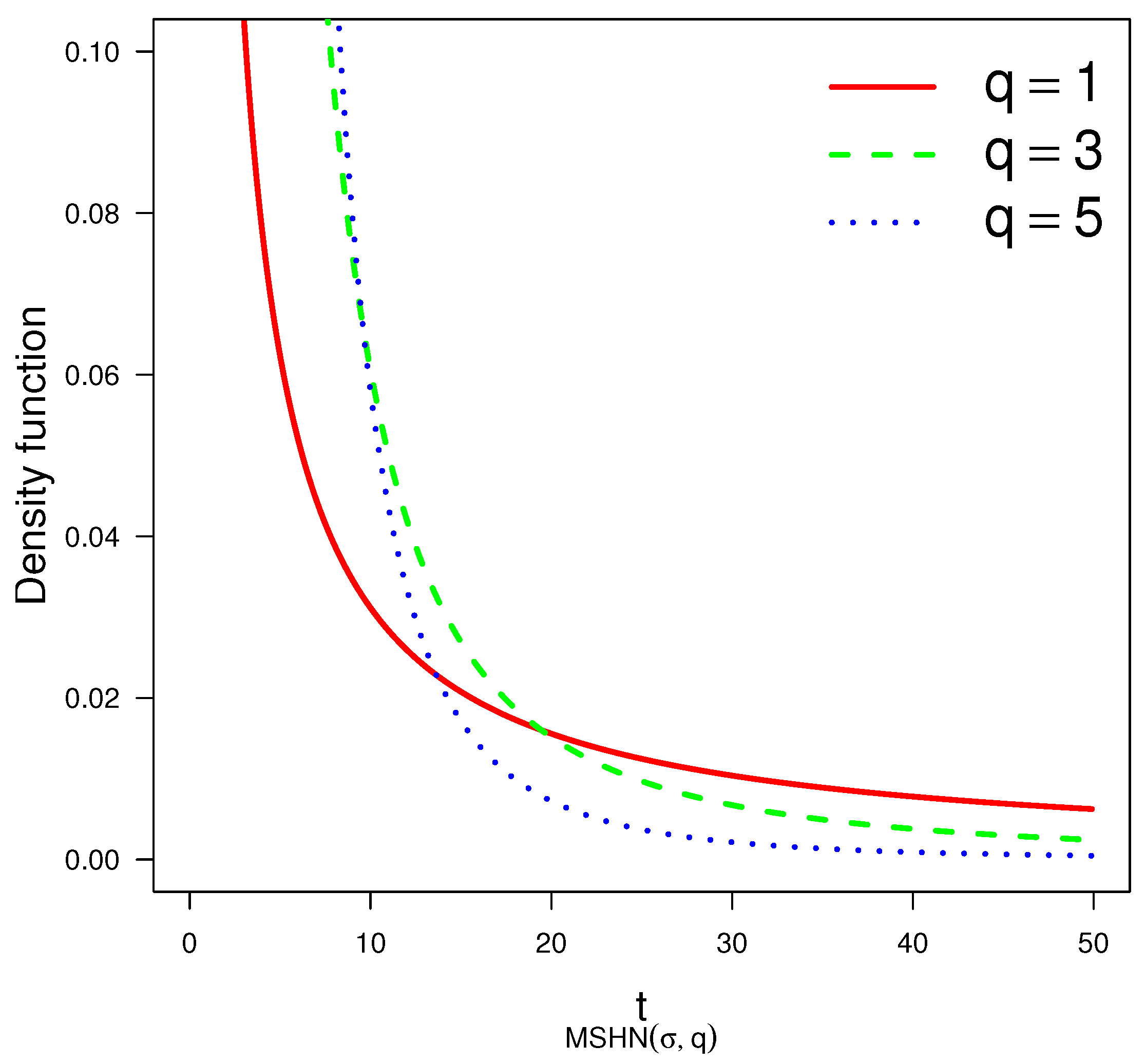
Figure 1 depicts plots of the density of the MSHN distribution for different values of parameter q.

We perform a brief comparison illustrating that the tails of the MSHN distribution are heavier than those of the SHN distribution.

Table 1. Tails comparison for different slashed half-normal (SHN) and modified slashed half-normal (MSHN) distributions.

Distribution	$\mathit{P}(\mathit{T}>3)$	$\mathit{P}(\mathit{T}>4)$	$\mathit{P}(\mathit{T}>5)$	$\mathit{P}(\mathit{T}>6)$	$\mathit{P}(\mathit{T}>7)$
SHN(1, 0.5)	0.3781	0.3497	0.3239	0.3009	0.2805
MSHN(1, 0.5)	0.5304	0.48289	0.4466	0.4176	0.3936
SHN(1, 1)	0.1777	0.1570	0.1385	0.1224	0.1086
MSHN(1, 1)	0.3678	0.2992	0.2519	0.2173	0.19102
SHN(1, 3)	0.0350	0.0205	0.0120	0.0044	0.0034
MSHN(1, 3)	0.0901	0.0438	0.0238	0.0142	0.0091

shows the tail probability for different values in the SHN and MSHN models. It is immediately apparent that the MSHN tails are heavier than those of the SHN distribution.

2.3. Properties

In this sub-section we study some properties of the MSHN distribution.

Proposition 2.

Let $T\sim MSHN(\sigma ,q)$, then when $\sigma =q=1$ the density is

$$f_T\left(t\right)=\frac{4}{t^2}\left(\frac{1}{\sqrt{2\pi }}-\frac{2}{t}exp(2/t^2)\mathsf{\Phi }\left(-\frac{2}{t}\right)\right),t>0,$$

(5)

where $\mathsf{\Phi }(·)$ is the cdf of the standard normal.

Proof. 

Using Proposition 1 for $\sigma =q=1$, we have,

$$f_T\left(t\right)=\frac{2}{\sqrt{2\pi }{t}^2}N\left(1,\frac{2}{z},\frac{1}{2},\frac{1}{2}\right)=\frac{2}{\sqrt{2\pi }{t}^2}{\int }_0^{\infty }exp\left(-\frac{2}{z}{x}^{1/2}-\frac{1}{2{\sigma }^2}x\right)dx,t>0.$$

(6)

Changing the variable $x=u^2$ we obtain the result. □

Proposition 3.

If $T|W=w\sim HN\left(\frac{\sigma }{w}\right)$ and $Y^{1/q}=W\sim Wei(q,1/2)$ then $T\sim MSHN(\sigma ,q)$.

Proof. 

Since the marginal pdf of T is given by

$$\begin{array}{c}\hfill f_T(t;\sigma ,q)={\int }_0^{\infty }{f}_{T|W}\left(t\right|w)f_W\left(w\right)dw=\frac{4q}{\sigma \sqrt{2\pi }}{\int }_0^{\infty }{w}^q{e}^{-\frac{w^2{t}^2}{2{\sigma }^2}-2w^q}dw,\end{array}$$

and using the Lemma 1 in the Appendix A, the result is obtained. □

Proposition 4.

Let $T\sim MSHN(\sigma ,q)$. If $q\to \infty$ then T converges in law to a random variable $T\sim HN\left(\sigma \right)$.

Proof. 

Let $T\sim MSHN(\sigma ,q)$ and $T=\frac{X}{Y^{1/q}}$, where $X\sim HN\left(\sigma \right)$ and $Y\sim Exp\left(2\right)$.

We study the convergence in law of T, since $Y\sim Exp\left(2\right)$ then $W=Y^{1/q}\sim Wei(q,1/2)$, we have that $E{\left(W-1\right)}^2=\frac{1}{2^{2/q}}\mathsf{\Gamma }(1+2/q)-\frac{2}{2^{1/q}}\mathsf{\Gamma }(1+1/q)+1$. If $q\to \infty$ then $E{\left(W-1\right)}^2\to 0$, i.e., we have $W\stackrel{\mathcal{P}}{⟶}$ 1 (see Lehmann [9]).

Since $T\sim MSHN(\sigma ,q)$, by applying Slutsky’s Lemma (see Lehmann [9]) to $T=\frac{X}{W}$, we have

$$T\stackrel{\mathcal{L}}{⟶}X\sim HN\left(\sigma \right),q\to \infty ,$$

(7)

that is, for increasing values of q, T converges in law to a $HN\left(\sigma \right)$ distribution. □

Remark 1.

Proposition 2 shows us that the $MSHN(1,1)$ distribution has a closed-form expression. Proposition 3 shows that an $MSHN(\sigma ,q)$ distribution can also be obtained as a scale mixture of an HN and a Wei distribution. This property is very important since it makes it possible to generate random numbers and implement the EM algorithm. Proposition 4 implies that, if $q\to \infty$ then the cdf of an $MSHN(\sigma ,q)$ model approaches to the cdf of a $HN\left(\sigma \right)$ distribution.

2.4. Moments

In this sub-section, the following proposition shows the computation of the moments of a random variable $T\sim MSHN(\sigma ,q)$. Hence, it also displays the coefficients of asymmetry and kurtosis.

Proposition 5.

Let $T\sim \mathrm{MSHN}(\sigma ,q)$. Then the r-th moment of T is given by

$${\mu }_r=\mathbb{E}\left(T^r\right)=\frac{2^{r\left(\frac{1}{q}+\frac{1}{2}\right)}}{\sqrt{\pi }}{\sigma }^r\mathsf{\Gamma }\left(\frac{r+1}{2}\right)\mathsf{\Gamma }\left(\frac{q-r}{q}\right),q>r,$$

(8)

where $\mathsf{\Gamma }(·)$ denotes the gamma function.

Proof. 

Let $W\sim Wei(q,1/2)$ and using Proposition 3, we have

$${\mu }_r=E\left(T^r\right)=E\left(E\left(X^r\right|W^r)\right)=E\left(\sqrt{\frac{2^r}{\pi }}\mathsf{\Gamma }\left(\frac{r+1}{2}\right){\sigma }^r{W}^{-r}\right)=\sqrt{\frac{2^r}{\pi }}\mathsf{\Gamma }\left(\frac{r+1}{2}\right){\sigma }^{r}E\left(W^{-r}\right),$$

where $E\left(W^{-r}\right)=2^{r/q}\mathsf{\Gamma }\left((q-r)/q\right)$, $q>r$ is the r-th moment of the inverse Weibull distribution. □

Corollary 1.

Let $T\sim \mathrm{MSHN}(\sigma ,q)$. Then the expectation and variance of T are given respectively by

$$E\left(T\right)=\frac{2^{\frac{1}{q}+\frac{1}{2}}}{\sqrt{\pi }}\sigma \mathsf{\Gamma }\left(\frac{q-1}{q}\right),q>1,\mathrm{and}$$

$$Var\left(T\right)=2^{\left(\frac{2}{q}+1\right)}{\sigma }^2\left[\frac{1}{2}\mathsf{\Gamma }\left(\frac{q-2}{q}\right)-\frac{1}{\pi }{\mathsf{\Gamma }}^2\left(\frac{q-1}{q}\right)\right],q>2.$$

Corollary 2.

Let $T\sim \mathrm{MSHN}(\sigma ,q)$. Then the coefficients of asymmetry (${\beta }_1$) and kurtosis (${\beta }_2$) are given by

$${\beta }_1=\frac{\frac{1}{\sqrt{\pi }}\mathsf{\Gamma }\left(\frac{q-3}{q}\right)-\frac{3}{2\sqrt{\pi }}\mathsf{\Gamma }\left(\frac{q-1}{q}\right)\mathsf{\Gamma }\left(\frac{q-2}{q}\right)+\frac{2}{\sqrt{{\pi }^3}}{\mathsf{\Gamma }}^3\left(\frac{q-1}{q}\right)}{{\left[\frac{1}{2}\mathsf{\Gamma }\left(\frac{q-2}{q}\right)-\frac{1}{\pi }{\mathsf{\Gamma }}^2\left(\frac{q-1}{q}\right)\right]}^{3/2}},q>3,\mathrm{and}$$

$${\beta }_2=\frac{\frac{3}{4}\mathsf{\Gamma }\left(\frac{q-4}{q}\right)-\frac{4}{\pi }\mathsf{\Gamma }\left(\frac{q-1}{q}\right)\mathsf{\Gamma }\left(\frac{q-3}{q}\right)+\frac{3}{\pi }{\mathsf{\Gamma }}^2\left(\frac{q-1}{q}\right)\mathsf{\Gamma }\left(\frac{q-2}{q}\right)-\frac{3}{{\pi }^2}{\mathsf{\Gamma }}^4\left(\frac{q-1}{q}\right)}{{\left[\frac{1}{2}\mathsf{\Gamma }\left(\frac{q-2}{q}\right)-\frac{1}{\pi }{\mathsf{\Gamma }}^2\left(\frac{q-1}{q}\right)\right]}^2},q>4.$$

Remark 2.

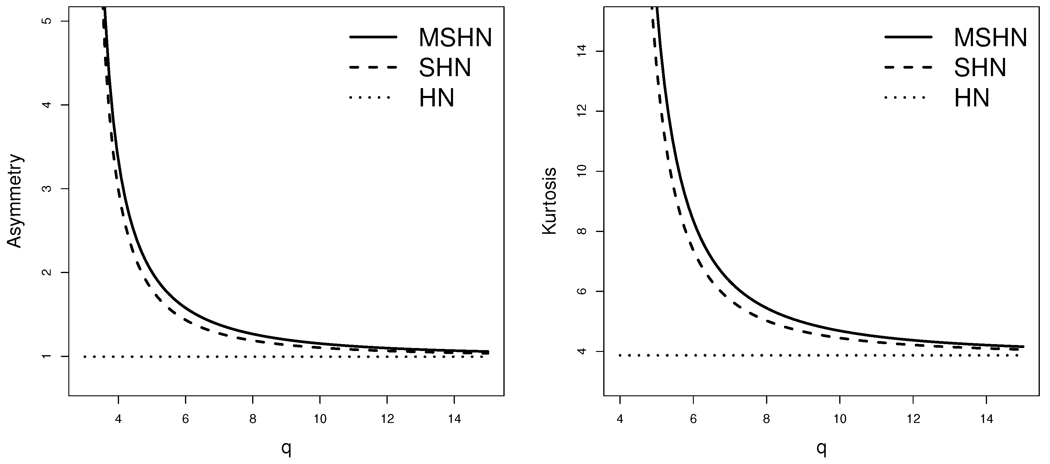
Figure 2 shows graphs of the coefficients of the MSHN distribution compared with those of the SHN distribution. Note that the MSHN distribution presents higher asymmetry and kurtosis values than the SHN distribution. Furthermore, in both distributions when $q\to \infty$ the coefficients of asymmetry and kurtosis converge to $\sqrt{2}(4-\pi ){(\pi -2)}^{-3/2}$ and $(3{\pi }^2-4\pi -12){(\pi -2)}^{-2}$, respectively; they coincide with the coefficients of the HN distribution.

3. Inference

Proposition 6.

Let $T_1,\cdots ,T_n$ be a random sample of size n of the $T\sim \mathrm{MSHN}(\sigma ,q)$ distribution. Then for $q>2$, the moment estimators of σ and q are given by

$$\begin{array}{c}\hfill {\widehat{\sigma }}_M=\frac{\sqrt{\pi }\overline{T}}{2^{\frac{1}{q}+\frac{1}{2}}\mathsf{\Gamma }\left(\frac{{\widehat{q}}_M-1}{{\widehat{q}}_M}\right)},\end{array}$$

(9)

$$\begin{array}{c}\hfill \pi {\overline{T}}^2\mathsf{\Gamma }\left(\frac{{\widehat{q}}_M-2}{{\widehat{q}}_M}\right)-2\overline{T^2}{\mathsf{\Gamma }}^2\left(\frac{{\widehat{q}}_M-1}{{\widehat{q}}_M}\right)=0,\end{array}$$

(10)

where $\overline{T}$ is the mean of the sample and $\overline{T^2}$ is the mean of the sample for the square of the observations.

Proof. 

From Proposition 5, and considering the first two equations in the moments method, we have

$$\overline{T}=\frac{2^{\frac{1}{q}+\frac{1}{2}}}{\sqrt{\pi }}\sigma \mathsf{\Gamma }\left(\frac{q-1}{q}\right)\mathrm{and}\overline{T^2}=2^{\frac{2}{q}}{\sigma }^2\mathsf{\Gamma }\left(\frac{q-2}{q}\right).$$

Solving the first equation above for $\sigma$ we obtain ${\widehat{\sigma }}_M$ given in (9). Substituting ${\widehat{\sigma }}_M$ in the second equation above, we obtain the result given in (10). □

4. Em Algorithm

The EM algorithm (Dempster et al. [10]) is a useful method for ML estimation in the presence of latent variables.

To facilitate the estimation process, we introduce latent variables $W_1,\cdots ,W_n$ through the following hierarchical representation of the MSHN model:

$$T_i\mid W_i=w_i\sim HN\left(\frac{\sigma }{w}\right)\mathrm{and}{W}_i\sim Wei(q,1/2).$$

In this setting, we have that

$$f_c\left(w\right|t)\propto w^{q}exp\left\{-\left(\frac{w^2{t}^2}{2{\sigma }^2}+2w^q\right)\right\}.$$

Therefore, the complete log-likelihood function can be expressed as

$${\displaystyle l_c\left(\theta \right|t_c)\propto -nlog\left(\sigma \right)-\sum _{i=1}^n\frac{w_i^2{t}_i^2}{2{\sigma }^2}+l_c\left(q\right|w_c),}$$

where ${\displaystyle l_c\left(q\right|w_c)=nlog\left(q\right)+q\sum _{i=1}^{n}log\left(w_i\right)-2\sum _{i=1}^n{w}_i^q}$.

Letting ${\widehat{w}}_i=\mathbb{E}\left[W_i\right|t_i,\mathbf{\theta }=\widehat{\mathbf{\theta }}]$, it follows that the conditional expectation of the complete log-likelihood function has the form

$$\begin{array}{ccc}\hfill Q(\mathbf{\theta }|\widehat{\mathbf{\theta }})& \propto & -nlog\left(\sigma \right)-\sum _{i=1}^n\frac{{\widehat{w}}_i^2{t}_i^2}{2{\sigma }^2}+Q(q|\widehat{\mathbf{\theta }}),\hfill \end{array}$$

(11)

where $Q(q|\widehat{\mathbf{\theta }})=nlog\left(q\right)+q{S}_{1n}-2S_{2n,q}$, with ${\displaystyle S_{1n}=\sum _{i=1}^n\mathbb{E}[log\left(W_i\right)|t_i]}$ and ${\displaystyle S_{2n,q}=\sum _{i=1}^n\mathbb{E}\left[W_i^q\right|t_i]}$.

As both quantities $S_{1n}$ and $S_{2n,q}$ have no explicit forms in the context of the MSHN model, they have to be computed numerically. Thus to compute $Q(q|\widehat{\mathbf{\theta }})$ we use an approach similar to that of Lee and Xu ([11], Section 3.1), i.e., considering $\{w_r;r=1,\dots ,R\}$ to be a random sample from the conditional distribution $W|(T=t,\mathbf{\theta }=\widehat{\mathbf{\theta }})$, then $Q(q|\widehat{\mathbf{\theta }})$ can be approximated as

$$Q(q|\widehat{\mathbf{\theta }})\approx \frac{1}{R}\sum _{r=1}^R{\ell }_c\left(q\right|w_r).$$

Therefore, the EM algorithm for the MSHN model is given by

• E-step: Given $\mathbf{\theta }={\widehat{\mathbf{\theta }}}^{\left(k\right)}={({\widehat{\sigma }}^{\left(k\right)},{\widehat{q}}^{\left(k\right)})}^{\top }$, calculate ${\widehat{w_i}}^{\left(k\right)}$, for $i=1,\cdots ,n.$
• CM-step I: Update ${\widehat{\sigma }}^{\left(k\right)}$

  $$\begin{array}{ccc}\hfill {\widehat{\sigma }}^{2(k+1)}& =& \frac{S_u^{\left(k\right)}}{2},\hfill \end{array}$$
• CM-step II: Fix $\alpha ={\widehat{\sigma }}^{(k+1)}$, update $q^{\left(k\right)}$ by optimizing ${\widehat{q}}^{(k+1)}=\arg {\max }_{\mathrm{q}}Q({\widehat{\sigma }}^{(k+1)},q|{\widehat{\mathbf{\theta }}}^{\left(k\right)})$, where ${\displaystyle S_u^{\left(k\right)}=\frac{1}{n}\sum _{i=1}^n{\widehat{w}}_i^{\left(k\right)}{t}_i.}$

The E, CM-I and CM-II steps are repeated until a convergence rule is satisfied, say $|l({\widehat{\mathbf{\theta }}}^{(k+1)})-l({\widehat{\mathbf{\theta }}}^{\left(k\right)})|$ is sufficiently small. Finally, standard errors (SE) can be estimated using the inverse of the observed information matrix.

Remark 3.

i. 

For $q\to \infty$, $\widehat{\sigma }$ in M-step reduces to those obtained when the HN distribution is used;

ii. 

An alternative to the CM-Steps II is obtained considering the idea in Lin et al. ([12], Section 3), by using the following estimation:

CML-step: Update $q^{\left(k\right)}$ by maximizing the constrained actual log-likelihood function, i.e.,

$$\begin{array}{ccc}\hfill {\widehat{q}}^{(k+1)}& =& {\displaystyle \arg {\max }_{\mathrm{q}}}\ell ({\widehat{\sigma }}^{(k+1)},q).\hfill \end{array}$$

5. Simulation

We present a simulation study to assess the performance of the EM algorithm for the parameters $\sigma$ and q in the MSHN model. We consider 1000 samples of three sample sizes generated from the MSHN model: $n=30$, 50 and 100. To generate $T\sim MSHN(\sigma ;q)$ the following algorithm was used:

• Simulate $X\sim N(0,{\sigma }^2)$ and $Y\sim Exp\left(2\right)$.
• Compute $T=\frac{\left|X\right|}{Y^{1/q}}$.

For each sample generated, the ML estimates were computed using the EM algorithm.

Table 2. Maximum likelihood (ML) estimations for parameters $\sigma$ and q of the MSHN distribution. Standard error (SE), root of the mean squared error (RMSE).

True Value			$\mathit{n}=30$			$\mathit{n}=50$			$\mathit{n}=100$
$\mathbf{\sigma }$	q	Estimator	Bias	SE	RMSE	Bias	SE	RMSE	Bias	SE	RMSE
1	1	$\sigma$	0.178	0.430	0.528	0.122	0.320	0.378	0.089	0.206	0.279
		q	0.199	0.422	0.668	0.097	0.219	0.263	0.059	0.138	0.163
	2	$\sigma$	0.111	0.355	0.407	0.078	0.258	0.295	0.042	0.172	0.186
		q	1.006	2.500	2.603	0.480	1.105	1.519	0.182	0.458	0.562
	5	$\sigma$	0.026	0.277	0.239	0.033	0.222	0.189	0.023	0.159	0.149
		q	2.227	8.833	3.871	2.012	6.743	3.550	1.333	4.092	2.905
2	1	$\sigma$	0.284	0.835	0.973	0.192	0.617	0.665	0.104	0.414	0.481
		q	0.168	0.356	0.571	0.094	0.215	0.263	0.058	0.141	0.166
	2	$\sigma$	0.294	0.727	0.815	0.122	0.507	0.572	0.074	0.343	0.383
		q	1.210	2.821	2.835	0.465	1.067	1.534	0.174	0.454	0.623
	5	$\sigma$	0.057	0.544	0.454	0.066	0.441	0.371	0.044	0.305	0.290
		q	2.456	8.991	3.934	2.089	6.712	3.615	1.545	4.150	3.075
5	1	$\sigma$	0.834	2.111	2.548	0.494	1.527	1.826	0.386	1.038	1.233
		q	0.217	0.414	0.740	0.119	0.225	0.287	0.083	0.144	0.174
	2	$\sigma$	0.658	1.782	2.065	0.293	1.285	1.475	0.209	0.872	0.966
		q	1.218	2.872	2.836	0.413	1.018	1.414	0.188	0.489	0.694
	5	$\sigma$	0.094	1.379	1.160	0.146	1.096	0.950	0.123	0.779	0.731
		q	2.266	8.894	3.880	1.952	6.526	3.557	1.370	4.118	2.948

shows the mean of the bias estimated for each parameter (bias), its SE and the estimated root of the mean squared error (RMSE). From Table 2, we conclude that the ML estimates are quite stable. The bias is reasonable and diminishes as the sample size is increased. As expected, the terms SE and RMSE are closer when the sample size is increased, suggesting that the SE of the estimators is well estimated.

6. Aplications

In this section we provide three applications to real datasets that illustrate the flexibility of the proposed model.

6.1. Application 1

Lyu [13] presents a data set related 104 times with programming in the Centre for Software Reliability (CSR). Some descriptive statistics are: mean = 147.8, variance = 60,071.7, skewness = 3, and kurtosis = 14.6. The moment estimators for the MSHN model were ${\widehat{\sigma }}_M=74.085$ and ${\widehat{q}}_M=2.402$, which were used as initial values to compute the $ML$ estimator in

Table 3. ML estimations with the corresponding SE for the models fitted. Half-normal (HN).

Parameters	HN (SE)	SHN (SE)	MSHN (SE)
$\widehat{\sigma }$	285.191 (19.774)	20.977 (5.674)	19.874 (4.867)
$\widehat{q}$	-	0.687 (0.118)	0.872 (0.115)
Log-likelihood	−663.411	−605.102	−600.876

.

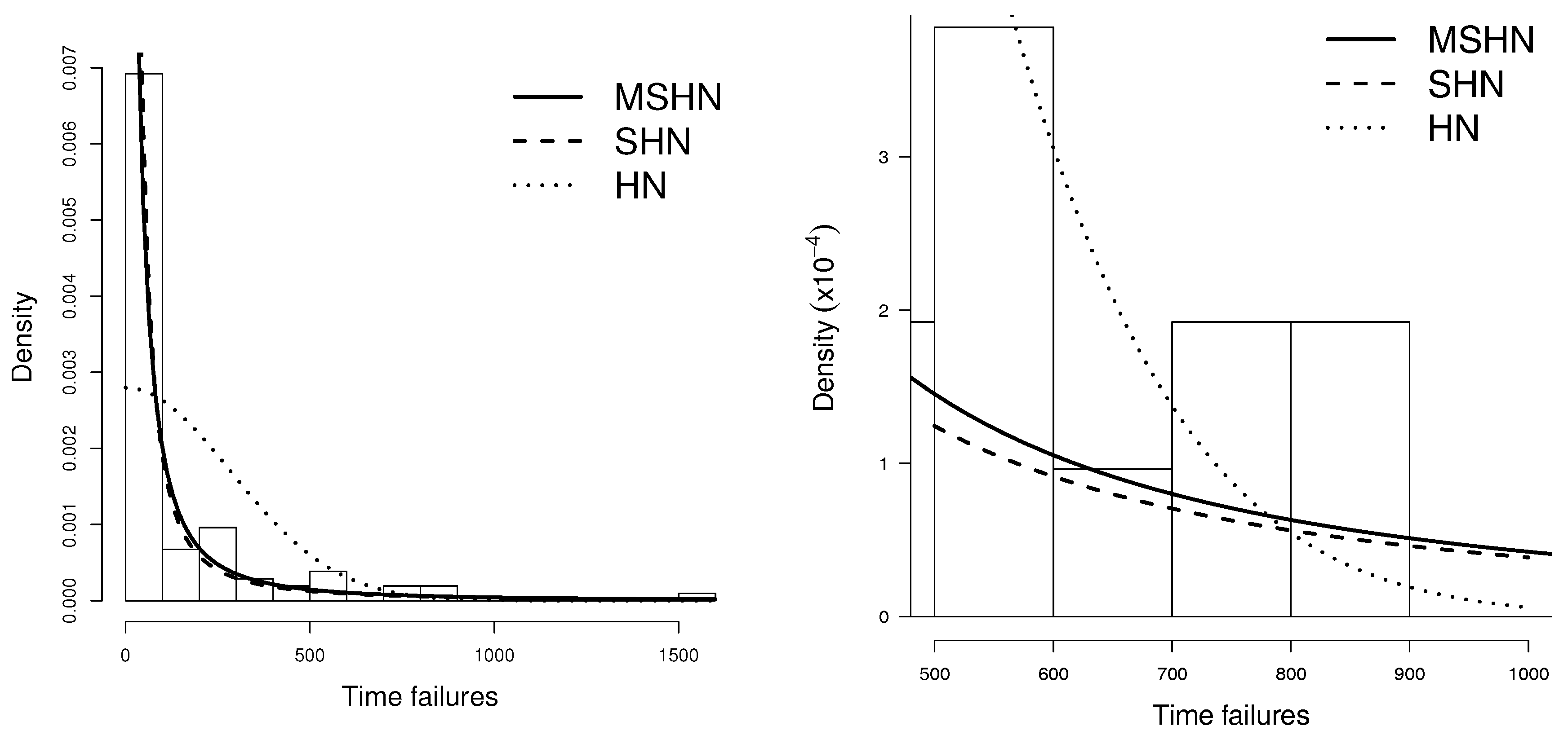
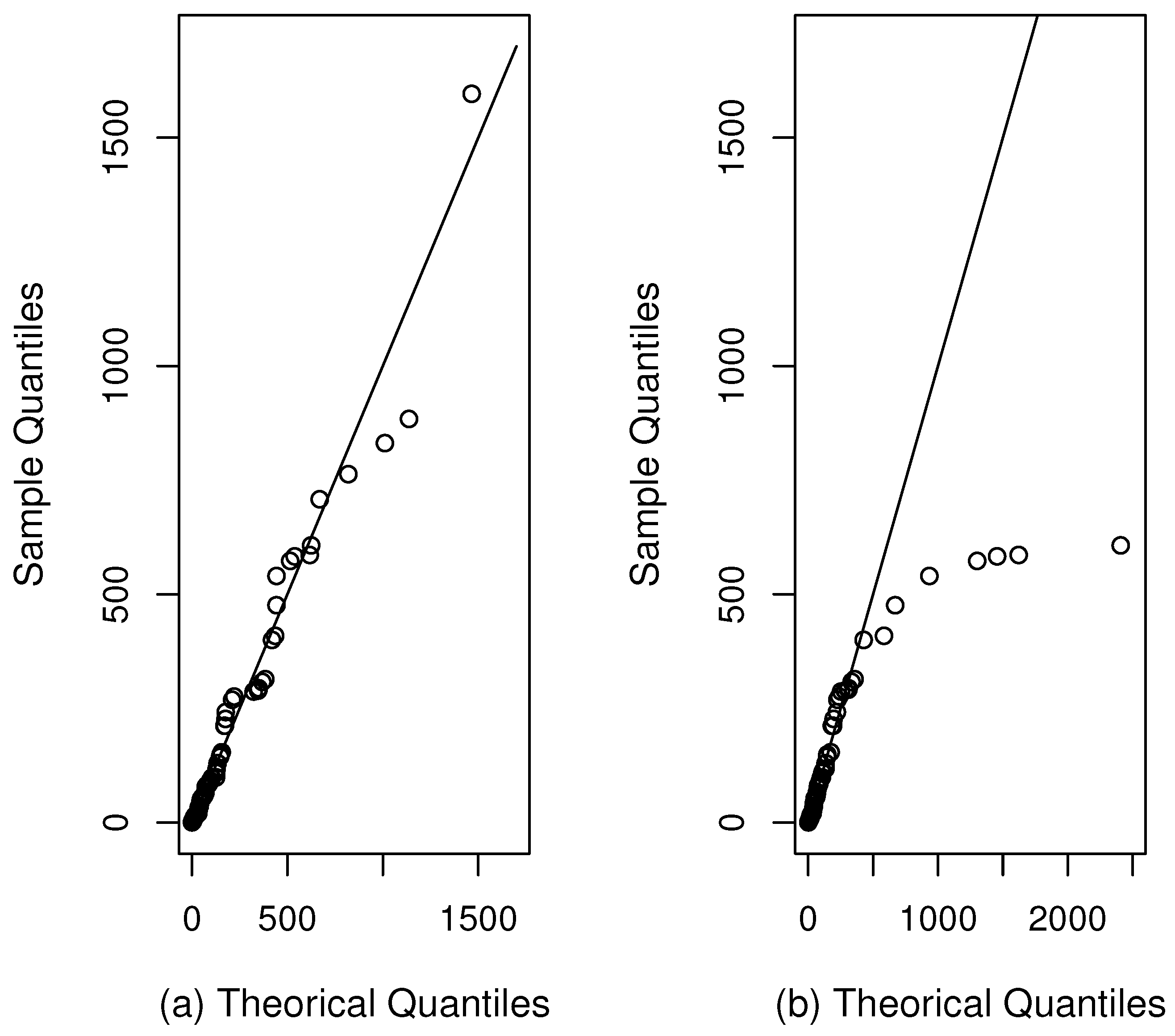
For each distribution we report the estimated log-likelihood. To compare the competing models, we consider the Akaike information criterion (AIC) (Akaike [14]) and the Bayesian information criterion (BIC) (Schwarz [15]), which are defined as $\mathrm{AIC}=2k-2log\mathrm{lik}$ and $\mathrm{BIC}=klog\left(n\right)-2log\mathrm{lik}$, respectively, where k is the number of parameters in the model, n is the sample size and $log\mathrm{lik}$ is the maximum value for the log-likelihood function.

Table 4. The Akaike information criterion (AIC) and the Bayesian information criterion (BIC) for each model fitted.

Criterion	HN	SHN	MSHN
AIC	1328.822	1214.204	1205.752
BIC	1331.466	1219.493	1211.041

displays the AIC and BIC for each model fitted. Figure 3 presents the histogram of the data fitted with the HN, SHN and MSHN distributions, provided with the ML estimations. The QQ-plot for the MSHN and SHN distributions are presented in Figure 4.

6.2. Application 2

The second dataset is taken from Von Alven [16], and represents 46 instances of active repairs (in hours) for an airborne communication transceiver. Some descriptive statistics are: mean = 3.607, variance = 24.445, skewness = 2.888, and kurtosis = 11.802.

Initially we computed the moment estimators for the MSHN distribution, obtaining the following estimations: ${\widehat{\sigma }}_M=2.407$ and ${\widehat{q}}_M=2.635$. We used these estimations as initial values in computing the ML estimators presented in

Table 5. ML estimations with the corresponding SE for the models fitted.

Parameters	HN (SE)	SHN (SE)	MSHN (SE)
$\widehat{\sigma }$	6.07 (0.6335)	1.6251 (0.4777)	1.5108 (0.3179)
$\widehat{q}$	-	1.3539 (0.4347)	1.6365 (0.3425)
Log-likelihood	−116.3881	−103.1834	−102.65

. For each distribution we report the estimated log-likelihood.

Table 6. AIC and BIC for each model fitted.

Criterion	HN	SHN	MSHN
AIC	234.7762	210.3668	209.302
BIC	236.6048	214.0241	212.9573

displays the AIC and BIC for each model fitted. Figure 5 presents the histogram of the data fitted with the HN, SHN and MSHN distributions, provided with the ML estimations.

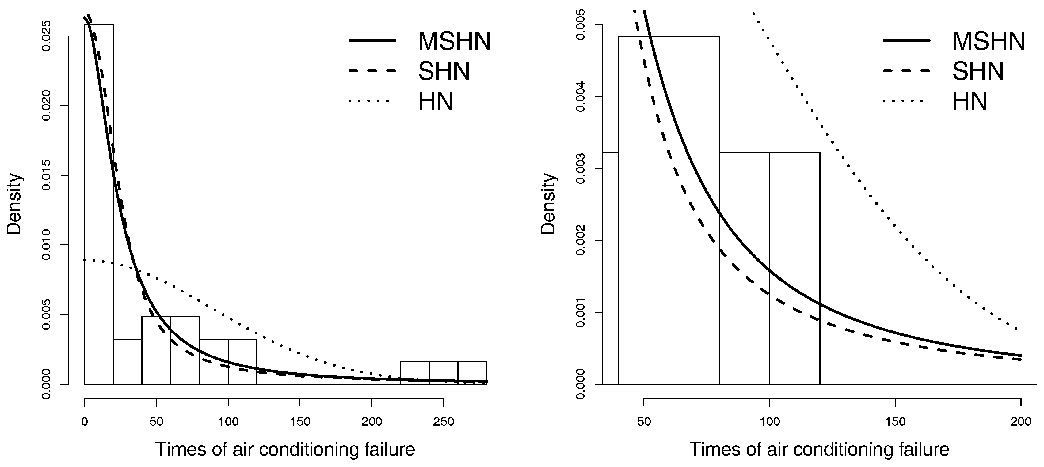
6.3. Application 3

The third data set (Linhart and Zucchini [17]) represents 31 times of air conditioning system failure of an aeroplane. Some descriptive statistics are: mean = 55.35, variance = 5132.503, skewness = 1.805, and kurtosis = 5.293.

Initially we computed the moment estimators for the MSHN distribution, and obtained the following estimations: ${\widehat{\sigma }}_M=38.125$ and ${\widehat{q}}_M=2.743$. We used these estimations as initial values in computing the ML estimators presented in

Table 7. ML estimations with the corresponding SE for the models fitted.

Parameters	HN (SE)	SHN (SE)	MSHN (SE)
$\widehat{\sigma }$	89.616 (11.381)	13.785 (6.047)	16.148(5.128)
$\widehat{q}$	-	0.859 (0.285)	1.233 (0.251)
Log-likelihood	−161.861	−154.857	−153.954

. For each distribution we report the estimated log-likelihood.

Table 8. AIC and BIC for each model fitted.

Criterion	HN	SHN	MSHN
AIC	325.7224	313.715	311.908
BIC	327.1564	316.583	314.776

displays the AIC and BIC for each model fitted. Figure 6 presents the histogram of the data fitted with the HN, SHN and MSHN distributions, provided with the ML estimations.

7. Conclusions

In this paper, we have introduced a new and more flexible model, as it increases kurtosis and contains, as a particular case, the HN distribution. The EM algorithm is implemented, obtaining acceptable results for the maximum likelihood estimators. In applications using real data it performs very well, better than competing models. Some further characteristics of the MSHN distribution are:

• The MSHN distribution has a greater kurtosis than the SHN distribution, as is clearly reflected in Table 1.
• The proposed model has a closed-form expression and presents more flexible asymmetry and kurtosis coefficients than that of the HN model.
• Two stochastic representations for the MSHN model are presented. One is defined as the quotient between two independent random variables: An HN in the numerator and Exp(2) in the denominator. The other shows that the MSHN distribution is a scale mixture of an HN and a Wei distribution.
• Using the mixed scale representation, the EM algorithm was implemented to calculate the ML estimators.
• Results from a simulation study indicate that with a reasonable sample size, an acceptable bias is obtained.
• Three illustrations using real data show that the MSHN model achieves a better fit in terms of the AIC and BIC criteria.

References

- Cooray, K.; Ananda, M.M.A. A Generalization of the Half-Normal Distribution with Applications to Lifetime Data. Commun. Stat. Theory Methods 2008, 37, 1323–1337. [Google Scholar] [CrossRef]
- Cordeiro, G.M.; Pescim, R.R.; Ortega, E.M.M. The Kumaraswamy Generalized Half-Normal Distribution for Skewed Positive Data. J. Data Sci. 2012, 10, 195–224. [Google Scholar]
- Gómez, Y.M.; Bolfarine, H. Likelihood-based inference for power half-normal distribution. J. Stat. Theory Appl. 2015, 14, 383–398. [Google Scholar] [CrossRef]
- Gómez, Y.M.; Vidal, I. A generalization of the half-normal distribution. Appl. Math. J. Chin. Univ. 2016, 31, 409–424. [Google Scholar] [CrossRef]
- Olmos, N.M.; Varela, H.; Gómez, H.W.; Bolfarine, H. An extension of the half-normal distribution. Stat. Pap. 2012, 53, 875–886. [Google Scholar] [CrossRef]
- Rogers, W.H.; Tukey, J.W. Understanding some long-tailed symmetrical distributions. Stat. Neerl. 1972, 26, 211–226. [Google Scholar] [CrossRef]
- Mosteller, F.; Tukey, J.W. Data Analysis And Regression; Addison-Wesley: Reading, MA, USA, 1977. [Google Scholar]
- Reyes, J.; Gómez, H.W.; Bolfarine, H. Modified slash distribution. Statistics 2013, 47, 929–941. [Google Scholar] [CrossRef]
- Lehmann, E.L. Elements of Large-Sample Theory; Springer: New York, NY, USA, 1999. [Google Scholar]
- Dempster, A.P.; Laird, N.M.; Rubin, D.B. Maximum likelihood from incomplete data via the EM algorithm. J. R. Statist. Soc. Ser. B 1977, 39, 1–38. [Google Scholar] [CrossRef]
- Lee, S.Y.; Xu, L. Influence analyses of nonlinear mixed-effects models. Comput. Stat. Data Anal. 2004, 45, 321–341. [Google Scholar] [CrossRef]
- Lin, T.I.; Lee, J.C.; Yen, S.Y. Finite mixture modeling using the skew-normal distribution. Stat. Sin. 2007, 17, 909–927. [Google Scholar]
- Lyu, M. Handbook of Software Reliability Engineering; IEEE Computer Society Press: Washington, DC, USA, 1996. [Google Scholar]
- Akaike, H. A new look at the statistical model identification. IEEE Trans. Auto. Contr. 1974, 19, 716–723. [Google Scholar] [CrossRef]
- Schwarz, G. Estimating the dimension of a model. Ann. Stat. 1978, 6, 461–464. [Google Scholar] [CrossRef]
- Von Alven, W.H. Reliability Engineering by ARINC; Prentice-Hall, Inc.: Upper Saddle River, NJ, USA, 1964. [Google Scholar]
- Linhart, H.; Zucchini, W. Model Selection; Wiley Series in Probability and Statistics; Wiley: Hoboken, NJ, USA, 1986. [Google Scholar]
- Prudnikov, A.P.; Brychkov, Y.A.; Marichev, O.I. Integrals and Series; Gordon & Breach Science Publishers: Amsterdam, The Netherlands, 1986. [Google Scholar]
Figure 1.
The density function for different values of parameter q and in the MSHN distribution.
Figure 2.
Graph of the coefficients of asymmetry and kurtosis for the MSHN and SHN distributions.
Figure 3.
Histogram fitted with the HN, SHN and MSHN distributions provided with the ML estimations.
Figure 4.
QQ plots: (a) MSHN distribution and (b) SHN distribution.
Figure 5.
Figure 6.