Generalized Truncation Positive Normal Distribution

Abstract

In this article we study the properties, inference, and statistical applications to a parametric generalization of the truncation positive normal distribution, introducing a new parameter so as to increase the flexibility of the new model. For certain combinations of parameters, the model includes both symmetric and asymmetric shapes. We study the model’s basic properties, maximum likelihood estimators and Fisher information matrix. Finally, we apply it to two real data sets to show the model’s good performance compared to other models with positive support: the first, related to the height of the drum of the roller and the second, related to daily cholesterol consumption.

1. Introduction

The half-normal (HN) distribution is a very important model in the statistical literature. Its density function has a closed-form and its cumulative distribution function (cdf) depends on the cdf of the standard normal model (or the error function), which is implemented in practically all mathematical and statistical software. Pewsey [1,2] provides the maximum likelihood (ML) estimation for the general location-scale HN distribution and its asymptotic properties. Wiper et al. [3] and Khan and Islam [4] perform analysis and applications for the HN model from a Bayesian framework. Moral et al. [5] also present the hnp R package, which produces half-normal plots with simulated envelopes using different diagnostics from a range of different fitted models. The HN model is also presented in the stochastic representation of the skew-normal distribution in Azzalini [6,7] and Henze [8]. In recent years this distribution has been used to model positive data, and it is becoming an important model in reliability theory despite the fact that it accommodates only decreasing hazard rates. Some of the generalizations of this distribution can be found in Cooray and Ananda [9], Olmos et al. [10], Cordeiro et al. [11], Gómez and Bolfarine [12], among others.

In particular, we focused on the extension of Cooray and Ananda [9]. The authors provided a motivation related to static fatigue life to consider the transformation $Z=\sigma Y^{1/\alpha }$, where $Y\sim HN\left(1\right)$. This model was named the generalized half-normal (GHN) distribution. An alternative way to extend the HN model was introduced by Gómez et al. [13] considering a normal distribution with mean and standard deviation $\mu$ and $\sigma$, respectively, truncated to the interval $(0,+\infty )$ and considering the reparametrization $\lambda =\mu /\sigma$. This model was named the truncated positive normal (TPN) distribution with density function given by

$$f(z;\sigma ,\lambda )=\frac{1}{\sigma \Phi \left(\lambda \right)}\varphi \left(\frac{z}{\sigma }-\lambda \right),z,\sigma >0,\lambda \in \mathbb{R},$$

(1)

where $\varphi (·)$ and $\Phi (·)$ denote the density and cdf of the standard normal models, respectively. We use $\mathrm{TPN}(\sigma ,\lambda )$ to refer to a random variable (r.v.) with density function as in Equation (1). Note that $\mathrm{TPN}(\sigma ,0)\equiv HN\left(\sigma \right)$.

In this work we consider a similar idea to that used in Cooray and Ananda [9] to extend the TPN model including the transformation $Y=\sigma X^{1/\alpha }$, where $X\sim TPN(1,\lambda )$. We will refer to this distribution as the generalized truncation positive normal (GTPN).

The rest of the manuscript is organized as follows. Section 2 is devoted to study of some important properties of the model, as well as its moments, quantile and hazard functions and its entropy. In Section 3 we perform an inference and present the Fisher information matrix for the proposed model. Section 4 discusses the selection model in nested and non-nested models for the GTPN distribution. In Section 5 we carry out a simulation study in order to study properties of the ML estimators in finite samples for the proposed distribution. Section 6 presents two applications to real data-sets to illustrate that the proposed model is competitive versus other common models for positive data in the literature. Finally, in Section 7, we present some concluding remarks.

2. Model Properties

In this section we introduce the main properties of the GTPN model such as density, quantile and hazard functions, moments, among others.

2.1. Stochastic Representation and Particular Cases

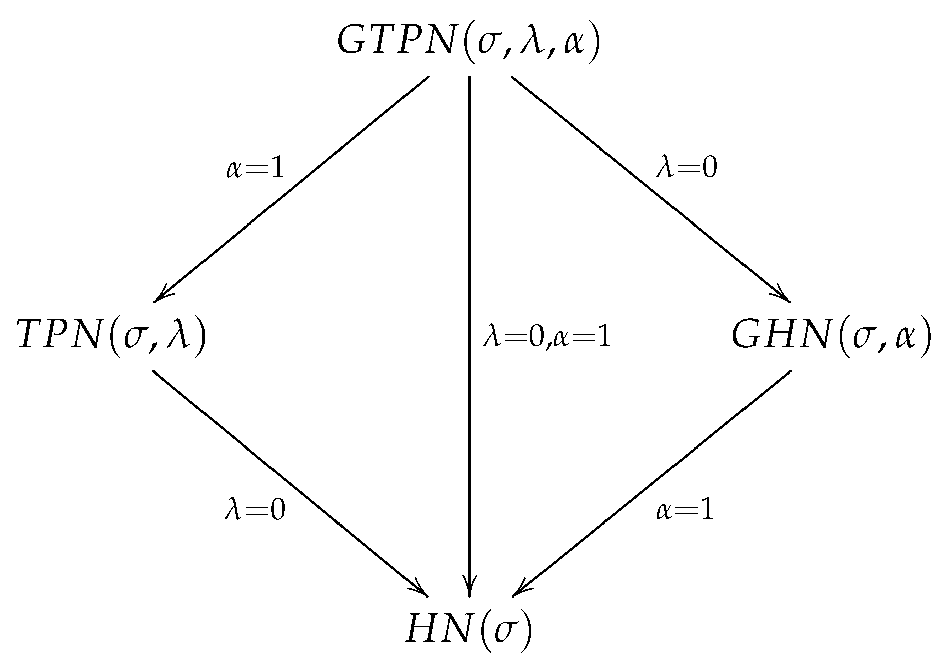
As mentioned previously, we say that a r.v. Z has $\mathrm{GTPN}(\sigma ,\lambda ,\alpha )$ distribution if $Z=\sigma Y^{1/\alpha }$, where $Y\sim TPN(1,\lambda )$. By construction, the following models are particular cases for the GTPN distribution:

• $\mathrm{GTPN}(\sigma ,\lambda ,\alpha =1)\equiv \mathrm{TPN}(\sigma ,\lambda )$.
• $\mathrm{GTPN}(\sigma ,\lambda =0,\alpha )\equiv \mathrm{GHN}(\sigma ,\alpha )$.
• $\mathrm{GTPN}(\sigma ,\lambda =0,\alpha =1)\equiv \mathrm{HN}\left(\sigma \right)$.

Figure 1 summarizes the relationships among the GTPN and its particular cases. We highlight that $\lambda =0$ and $\alpha =1$ are within the parametric space (not on the boundary). Therefore, to decide between the GTPN versus the TPN, GHN, or HN distributions we can use classical hypothesis tests such as the likelihood ratio test (LRT), score test (ST), or gradient test (GT).

2.2. Density, Cdf and Hazard Functions

Proposition 1.

For$Z\sim GTPN(\sigma ,\lambda ,\alpha )$, the density function is given by

$$f(z;\sigma ,\lambda ,\alpha )=\frac{\alpha }{{\sigma }^{\alpha }\Phi \left(\lambda \right)}{z}^{\alpha -1}\varphi \left({\left(\frac{z}{\sigma }\right)}^{\alpha }-\lambda \right),z\ge 0.$$

(2)

where$\sigma ,\alpha >0$and$\lambda \in \mathbb{R}$.

Proof. 

Considering the stochastic representation discussed in Section 2.1, we have that $z=g\left(y\right)=\sigma y^{1/\alpha }$ and

$$f_Z\left(z\right)=f_Y\left(g^{-1}\left(z\right)\right)\left|\frac{d{g}^{-1}\left(z\right)}{dz}\right|=\frac{1}{\Phi \left(\lambda \right)}\varphi (g^{-1}\left(z\right)-\lambda )\frac{\alpha z^{\alpha -1}}{{\sigma }^{\alpha }}.$$

Replacing $g^{-1}\left(z\right)={(z/\sigma )}^{\alpha }$ the result is obtained. □

Proposition 2.

For$Z\sim GTPN(\sigma ,\lambda ,\alpha )$, the cdf and hazard function are given by

$$F(z;\sigma ,\lambda ,\alpha )=\frac{\Phi ({\left(\frac{z}{\sigma }\right)}^{\alpha }-\lambda )+\Phi \left(\lambda \right)-1}{\Phi \left(\lambda \right)}andh\left(z\right)=\frac{f\left(z\right)}{1-F\left(z\right)}=\frac{\alpha z^{\alpha -1}\varphi \left({\left(\frac{z}{\sigma }\right)}^{\alpha }-\lambda \right)}{{\sigma }^{\alpha }\left[1-\Phi \left({\left(\frac{z}{\sigma }\right)}^{\alpha }-\lambda \right)\right]},$$

respectively, for all$z\ge 0$.

Figure 2 shows the density and hazard functions for the $\mathrm{GTPN}(\sigma =1,\lambda ,\alpha )$ model, considering some combinations for $(\lambda ,\alpha )$. Note that the GTPN model can assume decreasing and unimodal shapes for the density function and decreasing or increasing shapes for the hazard function.

2.3. Mode

Proposition 3.

The mode of the$GTPN(\sigma ,\lambda ,\alpha )$model is attained:

1. 

at$z=\frac{\sigma }{2^{1/\alpha }}{\left(\lambda +\sqrt{{\lambda }^2+4\left(1-\frac{1}{\alpha }\right)}\right)}^{1/\alpha }$whenever$\alpha \ge 1$or$0<\alpha <1$and$\lambda >0$,

2. 

at$z=0$in otherwise.

Proof. 

Let $l=log\left(f\right)$, where f is the density function defined in (2), of a direct computation we have

$$\frac{\partial l}{\partial z}=l_z=-\frac{1}{z}\left[\alpha {\left(\frac{z}{\sigma }\right)}^{2\alpha }-\alpha \lambda {\left(\frac{z}{\sigma }\right)}^{\alpha }-(\alpha -1)\right].$$

Note that $l_z$ vanishes when $\alpha {\left(\frac{z}{\sigma }\right)}^{2\alpha }-\alpha \lambda {\left(\frac{z}{\sigma }\right)}^{\alpha }-(\alpha -1)=0$. Using the auxiliary variable $w={\left(\frac{z}{\sigma }\right)}^{\alpha }$ the last equation is rewritten as follows:

$$\alpha w^2-\alpha \lambda w-(\alpha -1)=0.$$

(3)

In the rest of the proof we use the discriminant of the quadratic equation in Equation (3), which is given by $\Delta ={\alpha }^2{\lambda }^2+4\alpha (\alpha -1)={\alpha }^2[{\lambda }^2+4(1-\frac{1}{\alpha })]$ and its zeros are given by: $w=(\lambda \pm \sqrt{{\lambda }^2+4(1-\frac{1}{\alpha })})/2$.

If $\alpha \ge 1$ then $\Delta \ge {\lambda }^2$. In consequence, the mode is attained at $z_1=\frac{\sigma }{2^{1/\alpha }}{\left(\lambda +\sqrt{{\lambda }^2+4\left(1-\frac{1}{\alpha }\right)}\right)}^{1/\alpha }$.

If $0<\alpha <1$ then $\Delta <{\lambda }^2$. Here, two cases may occur. The first when $0<\Delta <{\lambda }^2$, in which case if $\lambda >0$ its mode is attained at $z=\frac{\sigma }{2^{1/\alpha }}{\left(\lambda +\sqrt{{\lambda }^2+4\left(1-\frac{1}{\alpha }\right)}\right)}^{1/\alpha }$, since $l_{zz}<0$, and if $\lambda <0$, then the zeros of Equation (3) are negative, implying that function l is strictly decreasing. Its mode is therefore attained at zero. The other case is when $\Delta <0$, then we have that $\alpha w^2-\alpha \lambda w-(\alpha -1)>0$ for all $w\ge 0$, implying that $l_z<0$ for all $z\ge 0$. Therefore, l is strictly decreasing and thus its mode is zero. □

Remark 1.

Note that$\alpha \ge 1$or$\lambda >0$implies that the mode of the GTPN model is attached in a positive value.

2.4. Quantiles

Proposition 4.

The quantile function for the$GTPN(\sigma ,\lambda ,\alpha )$is given by

$$Q\left(p\right)=\sigma {\left[{\Phi }^{-1}(1-(1-p)\Phi \left(\lambda \right))+\lambda \right]}^{\frac{1}{\alpha }}.$$

Proof. 

Follows from a direct computation, applying the definition of quantile function. □

Corollary 1.

The quartiles of the GTPN distribution are

1. 

First quartile$\sigma {[{\Phi }^{-1}(1-\frac{3}{4}\Phi \left(\lambda \right))+\lambda ]}^{\frac{1}{\alpha }}$.

2. 

Median$\sigma {[{\Phi }^{-1}(1-\frac{\Phi \left(\lambda \right)}{2})+\lambda ]}^{\frac{1}{\alpha }}$.

3. 

Third quartile$\sigma {[{\Phi }^{-1}(1-\frac{1}{4}\Phi \left(\lambda \right))+\lambda ]}^{\frac{1}{\alpha }}$.

2.5. Central Moments

Proposition 5.

Let$Z\sim GTPN(\sigma ,\lambda ,\alpha )$and$r=1,2,\dots$. The r-th non-central moment is given by

$${\mu }_r=\mathbb{E}\left(Z^r\right)=\frac{{\left(\sigma {\lambda }^{1/\alpha }\right)}^r{b}_r(\lambda ,\alpha )}{2\Phi \left(\lambda \right)\sqrt{\pi }},$$

where$b_r(\lambda ,\alpha )={\sum }_{k=0}^{\infty }\left(\genfrac{}{}{0pt}{}{r/\alpha }{k}\right){\left(\frac{\lambda }{2}\right)}^{-k}\Gamma \left(\frac{k+1}{2},\frac{{\lambda }^2}{2}\right)$and${\displaystyle \left(\genfrac{}{}{0pt}{}{r/\alpha }{k}\right)=\frac{1}{k!}{\displaystyle \prod _{n=1}^{k-1}}(r/\alpha -n)}$is the generalized binomial coefficient. When$r/\alpha \in \mathbb{N}$, the sum in$b_r(\lambda ,\alpha )$stops at$r/\alpha$.

Proof. 

Considering the stochastic representation of the GTPN model in Section 2.1, it is immediate that $\mathbb{E}\left(Z^r\right)={\sigma }^r\mathbb{E}\left(Y^{\frac{r}{\alpha }}\right)$, where $Y\sim TPN(1,\lambda )$. This expected value can be computed using Proposition 2.2 in Gómez et al. [13]. □

Remark 2.

When$r/\alpha \in \mathbb{N}$, Closed Forms Can Be Obtained for${\mu }_r$

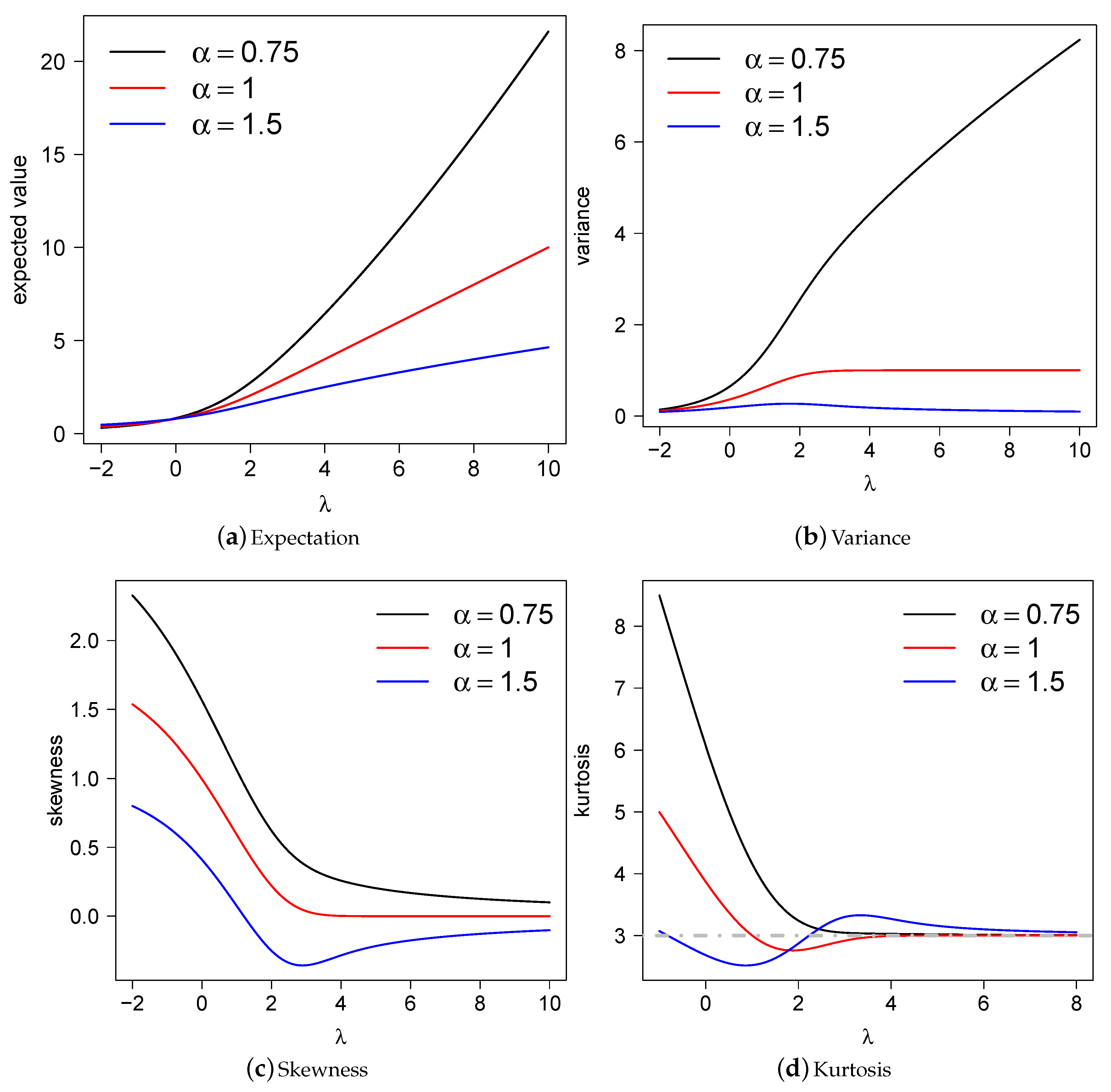
Figure 3 illustrates the mean, variance, skewness, and kurtosis coefficients for the $\mathrm{GTPN}(\sigma =1,\lambda ,\alpha )$ model for some combinations of its parameters.

2.6. Bonferroni and Lorenz Curves

In this subsection we present the Bonferroni and Lorenz curves (see Bonferroni [14]). These curves have applications not only in economics to study income and poverty, but also in medicine, reliability, etc. The Bonferroni curve is defined as

$$B\left(p\right)=\frac{1}{p\mu }{\int }_0^{q}zf\left(z\right)dz,0\le p<1.$$

where $\mu =E\left(Z\right)$, $q=F^{-1}\left(p\right)$. The Lorenz curve is obtained by the relation $L\left(p\right)=pB\left(p\right)$. Particularly, it can be checked that for the GTPN model the Bonferroni curve is given by

$$B\left(p\right)=\frac{1}{p\mu }\left[E\left(Z\right)-\frac{\sigma }{\Phi \left(\lambda \right)\sqrt{2\pi }}{\displaystyle \sum _{k=0}^{\infty }}\left(\genfrac{}{}{0pt}{}{\frac{1}{\alpha }}{k}\right){\lambda }^{\frac{1}{\alpha }-k}{2}^{\frac{k-1}{2}}\Gamma (\frac{k+1}{2},\frac{{\left({\left(\frac{q}{\sigma }\right)}^{\alpha }-\lambda \right)}^2}{2})\right].$$

These curves serve as graphic methods for analysis and comparison, e.g., the inequality of non-negative distributions. See, for example, for a more detailed discussion [15].

Figure 4 shows the Bonferroni curve for the $\mathrm{GTPN}(\sigma =1,\lambda ,\alpha )$ model, considering different values for $\lambda$ and $\alpha$.

2.7. Shannon Entropy

Shannon entropy (see Shannon [16]) measures the amount of uncertainty for a random variable. It is defined as:

$$S\left(Z\right)=-\mathbb{E}\left(logf\left(Z\right)\right).$$

Therefore, it can be checked that the Shannon entropy for the GTPN model is

$$S\left(Z\right)=log\left(\frac{\sqrt{2\pi \sigma \Phi \left(\lambda \right)}}{\alpha }\right)-(\alpha -1)\mathbb{E}\left(log\left(Z\right)\right)+\frac{{\mu }^{2\alpha }}{2{\sigma }^{2\alpha }}-\frac{\lambda {\mu }^{\alpha }}{{\sigma }^{\alpha }}+\frac{{\lambda }^2}{2},$$

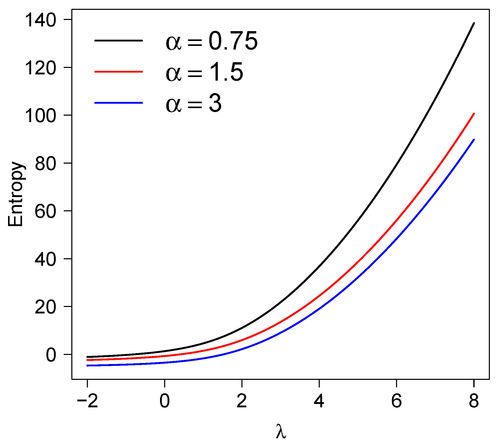
Figure 5 shows the entropy curve for the $\mathrm{GTPN}(\sigma =1.5,\lambda ,\alpha )$ model, considering different values for $\lambda$ and $\alpha$. We note that this function is increasing in $\lambda$ and $\alpha$. where ${\displaystyle \mathbb{E}\left(log\left(Z\right)\right)={\int }_0^{\infty }log\left(z\right)f(z;\sigma ,\lambda ,\alpha )dz}$. For $\alpha =1$, the Shannon entropy is reduced to

$$S\left(Z\right)=log\left(\sqrt{2\pi \sigma \Phi \left(\lambda \right)}\right)+\frac{{\mu }^2}{2{\sigma }^2}-\frac{\lambda \mu }{\sigma }+\frac{{\lambda }^2}{2},$$

which corresponds to the Shannon entropy for the TPN model; and for $\alpha =1$ and $\lambda =0$, $S\left(Z\right)$ is reduced to

$$S\left(Z\right)=log\left(\sqrt{\pi \sigma }\right)+\frac{{\mu }^2}{2{\sigma }^2},$$

which corresponds to the Shannon entropy for the HN distribution.

3. Inference

In this section we discuss the ML method for parameter estimation in the GTPN model.

3.1. Maximum Likelihood Estimators

For a random sample $z_1,\dots ,z_n$ from the $\mathrm{GTPN}(\sigma ,\lambda ,\alpha )$ model, the log-likelihood function for $\mathit{\theta }=(\sigma ,\lambda ,\alpha )$ is given by

$${\displaystyle \ell \left(\mathit{\theta }\right)=nlog\left(\alpha \right)+(\alpha -1){\displaystyle \sum _{i=1}^n}log\left(z_i\right)-n\alpha log\left(\sigma \right)-nlog(\Phi \left(\lambda \right))-\frac{n}{2}log\left(2\pi \right)-\frac{1}{2}{\displaystyle \sum _{i=1}^n}{\left({\left(\frac{z_i}{\sigma }\right)}^{\alpha }-\lambda \right)}^2.}$$

Therefore, the score assumes the form $S\left(\mathit{\theta }\right)=(S_{\sigma }\left(\mathit{\theta }\right),S_{\lambda }\left(\mathit{\theta }\right),S_{\alpha }\left(\mathit{\theta }\right))$, where

$$\begin{array}{cc}\hfill S_{\sigma }\left(\mathit{\theta }\right)& =-\frac{n\alpha }{\sigma }+{\displaystyle \sum _{i=1}^n}\left({\left(\frac{z_i}{\sigma }\right)}^{\alpha }-\lambda \right)\alpha {\left(\frac{z_i}{\sigma }\right)}^{\alpha -1}\frac{z_i}{{\sigma }^2},\hfill \\ \hfill S_{\lambda }\left(\mathit{\theta }\right)& =-n\xi \left(\lambda \right)+{\displaystyle \sum _{i=1}^n}\left({\left(\frac{z_i}{\sigma }\right)}^{\alpha }-\lambda \right)\mathrm{and}\hfill \\ \hfill S_{\alpha }\left(\mathit{\theta }\right)& =\frac{n}{\alpha }+{\displaystyle \sum _{i=1}^n}log{z}_i-nlog\left(\sigma \right)-{\displaystyle \sum _{i=1}^n}\left({\left(\frac{z_i}{\sigma }\right)}^{\alpha }-\lambda \right){\left(\frac{z_i}{\sigma }\right)}^{\alpha }log\left(\frac{z_i}{\sigma }\right),\hfill \end{array}$$

where $\xi \left(\lambda \right)=\frac{\varphi \left(\lambda \right)}{\Phi \left(\lambda \right)}$ is the negative of the inverse Mills ratio. The ML estimators are obtained by solving the equation $S\left(\mathit{\theta }\right)={\mathbf{0}}_3$, where ${\mathbf{0}}_p$ denotes a vector of zeros with dimension p. This equation has the following solution for $\lambda$

$$\widehat{\lambda }(\widehat{\sigma },\widehat{\alpha })=\frac{{\displaystyle {\displaystyle \sum _{i=1}^n}{\left(\frac{z_i}{\widehat{\sigma }}\right)}^{2\widehat{\alpha }}-n}}{{\displaystyle {\displaystyle \sum _{i=1}^n}{\left(\frac{z_i}{\widehat{\sigma }}\right)}^{\widehat{\alpha }}}}.$$

(4)

Replacing Equation (4) in $S_{\lambda }\left(\mathit{\theta }\right)=0$ and $S_{\alpha }\left(\mathit{\theta }\right)=0$, the problem is reduced to two equations. The solution of this problem needs to be solved by numerical methods such as Newton-Raphson. Below we discuss initial values for the vector $\mathit{\theta }$ to initialize the algorithm.

3.2. Initial Point to Obtain the Maximum Likelihood Estimators

In this subsection, we discuss the initial points for the iterative methods to find the ML estimators in the GTPN distribution.

3.2.1. A Naive Point Based on the HN Model

In Section 2 we discuss that $\mathrm{GTPN}(\sigma ,\lambda =0,\alpha =1)\equiv \mathrm{HN}\left(\sigma \right)$. Based on this fact, and considering that the ML estimator for $\sigma$ in the HN distribution has a closed-form, we can consider as an initial point ${\mathit{\theta }}_{naive}=\left({\displaystyle \sqrt{\frac{1}{n}\sum _{i=1}^n{z}_i^2},0,1}\right)$.

3.2.2. An Initial Point Based on Centiles

Let $q_t$, $t=1,\dots ,99$, the t-th sample centile based on $z_1,\dots ,z_n$. An initial point to $\mathit{\theta }$ can be obtained by matching $q_u,q_{50}$ and $q_{100-u}$, with $u\in \{1,2,\dots ,48,49\}$, with their respective theoretical counterparts. Defining $p=u/100$, the equations obtained are

$$\begin{array}{cc}\hfill q_u& =\sigma {\left[{\Phi }^{-1}(1-(1-p)\Phi \left(\lambda \right))+\lambda \right]}^{\frac{1}{\alpha }},q_{50}=\sigma {\left[{\Phi }^{-1}(1-0.5\Phi \left(\lambda \right))+\lambda \right]}^{\frac{1}{\alpha }}\mathrm{and}\hfill \\ \hfill q_{100-u}& =\sigma {\left[{\Phi }^{-1}(1-p\Phi \left(\lambda \right))+\lambda \right]}^{\frac{1}{\alpha }}.\hfill \end{array}$$

The solutions for $\sigma$ and $\alpha$ are

$$\tilde{\sigma }=\tilde{\sigma }(\tilde{\lambda })=\frac{q_{100-u}}{{\left[{\Phi }^{-1}\left(1-p\Phi (\tilde{\lambda })\right)+\tilde{\lambda }\right]}^{1/\tilde{\alpha }\left(\tilde{\lambda }\right)}}\mathrm{and}\tilde{\alpha }=\tilde{\alpha }\left(\tilde{\lambda }\right)=\frac{log\left(\frac{{\Phi }^{-1}\left(1-(1-p)\Phi \left(\tilde{\lambda }\right)\right)+\tilde{\lambda }}{{\Phi }^{-1}\left(1-p\Phi \left(\tilde{\lambda }\right)\right)+\tilde{\lambda }}\right)}{log\left(\frac{q_u}{q_{100-u}}\right)},$$

where $\tilde{\lambda }$ is obtained from the non-linear equation

$$\tilde{\sigma }\left(\tilde{\lambda }\right){\left[{\Phi }^{-1}\left(1-0.5\Phi \left(\tilde{\lambda }\right)\right)+\tilde{\lambda }\right]}^{1/\tilde{\alpha }\left(\tilde{\lambda }\right)}=q_{50}.$$

Therefore, the initial point based on this method is given by ${\mathit{\theta }}_{cent}=\left(\tilde{\sigma },\tilde{\lambda },\tilde{\alpha }\right)$.

3.3. An Initial Point Based on the Method of Moments

A more robust initial point can be obtained using the method of moments. The equations to solve are ${\mu }_r=\overline{z^r}$, $r=1,2,3$. The solution for $\sigma$ is

$${\tilde{\sigma }}^{\star }={\tilde{\sigma }}^{\star }({\tilde{\lambda }}^{\star },{\tilde{\alpha }}^{\star })=\frac{2\sqrt{\pi }\overline{z}\Phi \left({\tilde{\lambda }}^{\star }\right)}{{\left({\tilde{\lambda }}^{\star }\right)}^{1/{\tilde{\alpha }}^{\star }}{b}_1({\tilde{\lambda }}^{\star },{\tilde{\alpha }}^{\star })}.$$

The solution for $\lambda$ and $\alpha$ (say ${\tilde{\lambda }}^{\star }$ and ${\tilde{\alpha }}^{\star }$, respectively) are obtained from the non-linear equations

$$\frac{{\left({\tilde{\sigma }}^{\star }(\lambda ,\alpha ){\lambda }^{1/\alpha }\right)}^2{b}_2(\alpha ,\lambda )}{2\Phi \left(\lambda \right)\sqrt{\pi }}=\overline{z^2}\mathrm{and}\frac{{\left({\tilde{\sigma }}^{\star }(\lambda ,\alpha ){\lambda }^{1/\alpha }\right)}^3{b}_3(\alpha ,\lambda )}{2\Phi \left(\lambda \right)\sqrt{\pi }}=\overline{z^3}.$$

Therefore, the initial point based on this method is given by ${\mathit{\theta }}_{mom}=\left({\tilde{\sigma }}^{\star },{\tilde{\lambda }}^{\star },{\tilde{\alpha }}^{\star }\right)$.

3.4. Fisher Information Matrix

The Fisher information (FI) matrix for the GTPN distribution is given by $IF\left(\mathit{\theta }\right)={\left(I_{ab}\right)}_{a,b\in \{\sigma ,\lambda ,\alpha \}}$. Consider the notation

$$T_{jk}=T_{jk}\left(\lambda \right)={\int }_0^{\infty }{[log\left(w\right)]}^k{w}^j\varphi (w-\lambda )dw,j\in \{1,2\},k\in \{0,1,2\}.$$

Therefore,

$$\begin{array}{cc}\hfill I_{\sigma \sigma }& =-\frac{\alpha }{{\sigma }^2}+\frac{\alpha (2\alpha +1)}{{\sigma }^2\Phi \left(\lambda \right)}{T}_{20}-\frac{\lambda \alpha (\alpha +1)}{{\sigma }^2\Phi \left(\lambda \right)}{T}_{10},\hfill \\ \hfill I_{\sigma \lambda }& =\frac{\alpha }{\sigma \Phi \left(\lambda \right)}{T}_{10},\hfill \\ \hfill I_{\sigma \alpha }& =\frac{1}{\sigma }+\frac{1}{\sigma \Phi \left(\lambda \right)}[\lambda (T_{10}+T_{11})-T_{20}-2T_{21}],\hfill \\ \hfill I_{\lambda \lambda }& =1-\lambda \xi \left(\lambda \right)-{\xi }^2\left(\lambda \right),\hfill \\ \hfill I_{\lambda \alpha }& =-\frac{1}{\alpha \Phi \left(\lambda \right)}{T}_{11},\hfill \\ \hfill I_{\alpha \alpha }& =\frac{1}{{\alpha }^2}+\frac{2}{{\alpha }^2\Phi \left(\lambda \right)}{T}_{22}-\frac{\lambda }{{\alpha }^2\Phi \left(\lambda \right)}{T}_{12}\hfill \end{array}$$

We observe that $T_{jk}\left(\lambda \right)$ is a continuous function and ${lim}_{\left|\lambda \right|\to +\infty }{T}_{jk}\left(\lambda \right)=0$, then $T_{jk}\left(\lambda \right)<+\infty$. Note that for $\lambda =0$ and $\alpha =1$ this matrix is reduced to

$$FI(\sigma ,0,1)=\left(\begin{array}{ccc}\frac{2}{{\sigma }^2}& \frac{1}{\sigma }\sqrt{\frac{2}{\pi }}& -\frac{4}{\sigma }{\widehat{T}}_{21}\\ ·& 1-\frac{2}{\pi }& -2{\widehat{T}}_{11}\\ ·& ·& 1+4{\widehat{T}}_{22}\end{array}\right),$$

where ${\widehat{T}}_{jk}=T_{jk}\left(0\right)$. Additionally, we note that

$$\det \left(FI(\sigma ,0,1)\right)=\frac{2}{{\sigma }^2}\left[\frac{(\pi -3)}{\pi }(1+4{\widehat{T}}_{22}+4{\widehat{T}}_{21})-4{({\widehat{T}}_{11}-\sqrt{\frac{2}{\pi }}{\widehat{T}}_{21})}^2\right]\approx \frac{0.1021506}{{\sigma }^2}>0,\forall \sigma >0,$$

where $\det (·)$ denotes the determinant operator. Therefore, the FI matrix for the reduced model (HN) is invertible.

4. Model Discrimination

In this section we discuss some techniques to discriminate among the GTPN distribution and other models.

4.1. GTPN Versus Submodels

An interesting problem to solve is the discrimination between GTPN and the three submodels represented in Figure 1. In other words, we are interested in testing the following hypotheses:

• $H_0^{\left(1\right)}:\alpha =1$ versus $H_1^{\left(1\right)}:\alpha \ne 1$ (TPN versus GTPN distribution).
• $H_0^{\left(2\right)}:\lambda =0$ versus $H_1^{\left(2\right)}:\lambda \ne 0$ (GHN versus GTPN distribution).
• $H_0^{\left(3\right)}:(\alpha ,\lambda )=(1,0)$ versus $H_1^{\left(3\right)}:(\alpha ,\lambda )\ne (1,0)$ (HN versus GTPN distribution).

The three hypotheses can be tested considering the LRT, ST, and GT. Below we present the statistics for the three tests considered and for the three hypotheses of interest.

4.1.1. Likelihood Ratio Test

The statistic for the LRT (say SLR) to tests $H_0^{\left(j\right)}$, $j=1,2,3$, is defined as

$${\mathrm{SLR}}_j=2\left[\ell \left(\widehat{\sigma },\widehat{\lambda },\widehat{\alpha }\right)-\ell \left({\widehat{\sigma }}_{0j},{\widehat{\lambda }}_{0j},{\widehat{\alpha }}_{0j}\right)\right],$$

where ${\widehat{\sigma }}_{0j},{\widehat{\lambda }}_{0j}$ and ${\widehat{\alpha }}_{0j}$ denote the ML estimators for $\sigma$, $\lambda$ and $\alpha$ restricted to $H_0^{\left(j\right)}$, $j=1,2,3$. Under $H_0^{\left(j\right)}$, $j=1,2$, ${\mathrm{SLR}}_j\sim {\chi }_{\left(1\right)}^2$ and under $H_0^{\left(3\right)}$, ${\mathrm{SLR}}_3\sim {\chi }_{\left(2\right)}^2$, where ${\chi }_{\left(p\right)}^2$ denotes the Chi-squared distribution with p degrees of freedom. For $H_0^{\left(3\right)}$, we obtain

$${\widehat{\sigma }}_{03}=\sqrt{\frac{1}{n}\sum _{i=1}^n{z}_i^2},{\widehat{\lambda }}_{03}=0\mathrm{and}{\widehat{\alpha }}_{03}=1,$$

whereas to test $H_0^{\left(1\right)}$ and $H_0^{\left(2\right)}$ the ML estimators under the null hypotheses need to be computed numerically. However, in both cases the problem is reduced to a unidimensional maximization. For details see Cooray and Ananda [9] and Gómez et al. [13], respectively.

4.1.2. Score Test

The statistic for the ST (say SR) to test $H_0^{\left(j\right)}$, $j=1,2,3$, is defined as

$${\mathrm{SR}}_j={\left[S\left({\widehat{\theta }}_{0j}\right)\right]}^{\top }{\left[IF\left({\widehat{\theta }}_{0j}\right)\right]}^{-1}S\left({\widehat{\theta }}_{0j}\right),$$

where ${\widehat{\mathit{\theta }}}_j$ is the ML estimator under $H_0^{\left(j\right)}$. Under $H_0^{\left(j\right)}$, $j=1,2$, ${\mathrm{SR}}_j\sim {\chi }_{\left(1\right)}^2$ and under $H_0^{\left(3\right)}$, ${\mathrm{SR}}_3\sim {\chi }_{\left(2\right)}^2$.

4.1.3. Gradient Test

The statistic for the GT (say ST) to tests $H_0^{\left(j\right)}$, $j=1,2,3$, is defined as

$${\mathrm{ST}}_j=S\left({\widehat{\mathit{\theta }}}_j\right)\left(\widehat{\mathit{\theta }}-{\widehat{\mathit{\theta }}}_j\right).$$

Again, under $H_0^{\left(j\right)}$, $j=1,2$, ${\mathrm{ST}}_j\sim {\chi }_{\left(1\right)}^2$ and under $H_0^{\left(3\right)}$, ${\mathrm{ST}}_3\sim {\chi }_{\left(2\right)}^2$. After some algebraic manipulations, we obtain that

$$\begin{array}{cc}\hfill {\mathrm{ST}}_1& =\left(\widehat{\alpha }-1\right)\left\{n\left[1-log\left({\widehat{\sigma }}_{01}\right)\right]+{\displaystyle \sum _{i=1}^n}\left[log{z}_i-\left(\left(\frac{z_i}{{\widehat{\sigma }}_{01}}\right)-{\widehat{\lambda }}_{01}\right)\left(\frac{z_i}{{\widehat{\sigma }}_{01}}\right)log\left(\frac{z_i}{{\widehat{\sigma }}_{01}}\right)\right]\right\}.\hfill \\ \hfill {\mathrm{ST}}_2& =\widehat{\lambda }\left[-n\sqrt{\frac{2}{\pi }}+{\displaystyle \sum _{i=1}^n}{\left(\frac{z_i}{{\widehat{\sigma }}_{02}}\right)}^{{\widehat{\alpha }}_{02}}\right].\hfill \\ \hfill {\mathrm{ST}}_3& =\left(\widehat{\alpha }-1\right)\left\{n\left[1-log\left({\widehat{\sigma }}_{03}\right)\right]+{\displaystyle \sum _{i=1}^n}\left[log{z}_i-{\left(\frac{z_i}{{\widehat{\sigma }}_{03}}\right)}^{2}log\left(\frac{z_i}{{\widehat{\sigma }}_{03}}\right)\right]\right\}+\widehat{\lambda }\left[-n\sqrt{\frac{2}{\pi }}+{\displaystyle \sum _{i=1}^n}\left(\frac{z_i}{{\widehat{\sigma }}_{03}}\right)\right].\hfill \end{array}$$

4.2. Non-Nested Models

The comparison of non-nested models can be performed based on the AIC criteria (Akaike [17]), where the model with a lower AIC is preferred. However, in practice we can have a set of inappropriate models for a certain data set. For this reason, we also need to perform a goodness-of-fit validation. This can be performed, for instance, based on the quantile residuals (QR). For more details see Dunn and Smyth [18]. These residuals are defined as

$$Q{R}_i=G(z_i;\widehat{\psi }),i=1,\dots ,n,$$

where $G(;\widehat{\psi })$ is the cdf of the specified distribution evaluated in the estimator for $\psi$. If the model is correctly specified, such residuals are a random sample from the standard normal distribution. This can be assessed using, for instance, the Anderson–Darling (AD), Cramer-Von-Mises (CVM) and Shapiro–Wilks (SW) tests. A discussion of these tests can be seen in Yazici and Yocalan [19].

5. Simulation

In this section we present a Monte Carlo (MC) simulation study in order to illustrate the behavior of the ML estimators. We consider three sample sizes: $n=50,150$ and 300; two values for $\sigma$:1 and 2; two values for $\lambda$:3 and 4; and three values for $\alpha$: $0.8,1$ and 2. For each combination of n, $\sigma$, $\lambda$ and $\alpha$, we draw 10,000 samples of size n from the $\mathrm{GTPN}(\sigma ,\lambda ,\alpha )$ model. To simulate a value from this distribution, we consider the following scheme:

• Simulate $X\sim Uniform(0,1)$.
• Compute $Y={\Phi }^{-1}(1+(X+1)\Phi \left(\lambda \right))+\lambda$.
• Compute $Z=\sigma Y^{\frac{1}{\alpha }}$.

For each sample generated, ML estimators were computed numerically using the Newton-Raphson algorithm.

Table 1. Monte Carlo (MC) simulation study for the maximum likelihood (ML) estimators in the $(\mathrm{GTPN}\sigma ,\lambda ,\alpha )$ model in 12 combinations of $\sigma$, $\lambda$ and $\alpha$. The results summarize the mean and the standard deviation (sd) of the respective estimators obtained in the 10,000 replicates.

			n = 50						n = 150						n = 300						n = 1000
True Valor			$\widehat{\mathit{\sigma }}$		$\widehat{\mathit{\lambda }}$		$\widehat{\mathit{\alpha }}$		$\widehat{\mathit{\sigma }}$		$\widehat{\mathit{\lambda }}$		$\widehat{\mathit{\alpha }}$		$\widehat{\mathit{\sigma }}$		$\widehat{\mathit{\lambda }}$		$\widehat{\mathit{\alpha }}$		$\widehat{\mathit{\sigma }}$		$\widehat{\mathit{\lambda }}$		$\widehat{\mathit{\alpha }}$
$\mathit{\sigma }$	$\mathit{\lambda }$	$\mathit{\alpha }$	mean	sd	mean	sd	mean	sd	mean	sd	mean	sd	mean	sd	mean	sd	mean	sd	mean	sd	mean	sd	mean	sd	mean	sd
1	3	0.8	1.523	1.573	3.089	1.797	0.987	1.029	1.227	1.029	3.000	1.052	0.875	0.350	1.081	0.614	3.017	0634	0.830	0.202	1.011	0.233	3.014	0.267	0.803	0.071
		1	1.286	1.105	3.118	1.843	1.227	0.705	1.111	0.705	3.027	1.040	1.083	0.425	1.044	0.444	3.020	0.629	1.031	0.250	1.006	0.185	3.012	0.266	1.004	0.089
		2	1.006	0.510	3.220	2.036	2.432	0.309	1.011	0.309	3.019	1.055	2.171	0.850	1.001	0.196	3.022	0.614	2.058	0.481	0.998	0.093	3.013	0.266	2.008	0.177
	4	0.8	1.489	1.799	4.391	2.010	0.971	0.860	1.087	0.860	4.280	1.199	0.817	0.282	1.017	0.513	4.164	0.786	0.798	0.148	1.003	0.301	4.049	0.413	0.799	0.082
		1	1.236	1.219	4.439	2.182	1.203	0.631	1.018	0.631	4.295	1.222	1.017	0.343	0.986	0.418	4.187	0.826	0.995	0.191	0.993	0.230	4.055	0.404	0.998	0.099
		2	0.962	0.543	4.642	2.495	2.360	0.321	0.957	0.321	4.323	1.326	2.033	0.696	0.974	0.223	4.168	0.839	2.000	0.382	0.993	0.118	4.045	0.404	2.000	0.198
2	3	0.8	3.006	3.131	3.157	1.876	0.974	1.996	2.423	1.996	3.018	1.045	0.869	0.340	2.152	1.185	3.023	0.624	0.823	0.194	2.034	0.472	3.007	0.269	0.805	0.072
		1	2.512	2.198	3.215	1.942	1.207	1.437	2.237	1.437	3.028	1.077	1.086	0.431	2.094	0.897	3.017	0.642	1.033	0.250	2.009	0.373	3.015	0.269	1.004	0.089
		2	1.999	1.039	3.318	2.223	2.417	0.631	2.017	0.631	3.035	1.096	2.171	0.862	2.000	0.405	3.027	0.638	2.061	0.504	1.995	0.186	3.016	0.267	2.006	0.177
	4	0.8	2.880	3.544	4.562	2.283	0.970	1.714	2.161	1.714	4.326	1.288	0.813	0.282	2.024	1.078	4.194	0.849	0.796	0.160	2.003	0.573	4.053	0.404	0.799	0.079
		1	2.402	2.434	4.659	2.419	1.176	1.283	2.033	1.283	4.344	1.346	1.015	0.355	1.974	0.835	4.190	0.844	0.995	0.191	1.990	0.465	4.053	0.408	0.998	0.100
		2	1.913	1.132	4.802	2.848	2.378	0.668	1.898	0.668	4.393	1.469	2.024	0.708	1.938	0.460	4.198	0.901	1.993	0.391	1.984	0.236	4.047	0.401	2.000	0.198

presents means and standard deviations for each parameter in each case. Notice that bias and standard deviations are reduced as the sample size increases, suggesting that the ML estimators are consistent.

6. Applications

In this section we present two real data applications to illustrate the better performance of the GTPN model over other well known models in the literature. For these comparisons we also consider the Weibull (WEI) and the Generalized Lindley (GL, Zakerzadeh [20]) models. The density function of the Weibull distribution is given by

$$f(x;\sigma ,\lambda )=\frac{\sigma }{\lambda }{x}^{\sigma -1}{e}^{-x^{\sigma }/\lambda },$$

with $x>0$, $\sigma >0$ and $\lambda >0$, whereas for the GL model is given by

$$f(x;\alpha ,\theta ,\gamma )=\frac{{\theta }^2{\left(\theta x\right)}^{\alpha -1}(\alpha +\gamma x)e^{-\theta x}}{(\gamma +\theta )\Gamma (\alpha +1)},$$

with $x>0$, $\theta >0$ $\alpha >0$ and $\gamma >0$.

6.1. Application 1

The data set was taken from Laslett [21], and consisted of $n=115$ heights measured at 1 micron intervals along the drum of a roller (i.e., parallel to the axis of the roller). This was part of an extensive study of the surface roughness of the rollers. A statistical summary of the data set is presented in

Table 2. Descriptive statistics of the Laslett data set.

Dataset	n	$\overline{\mathit{X}}$	S2	$\sqrt{{\mathit{b}}_{\mathbf{1}}}$	${\mathit{b}}_{\mathbf{2}}$
Heights measured	115	3.48	0.52	−1.24	6.30

.

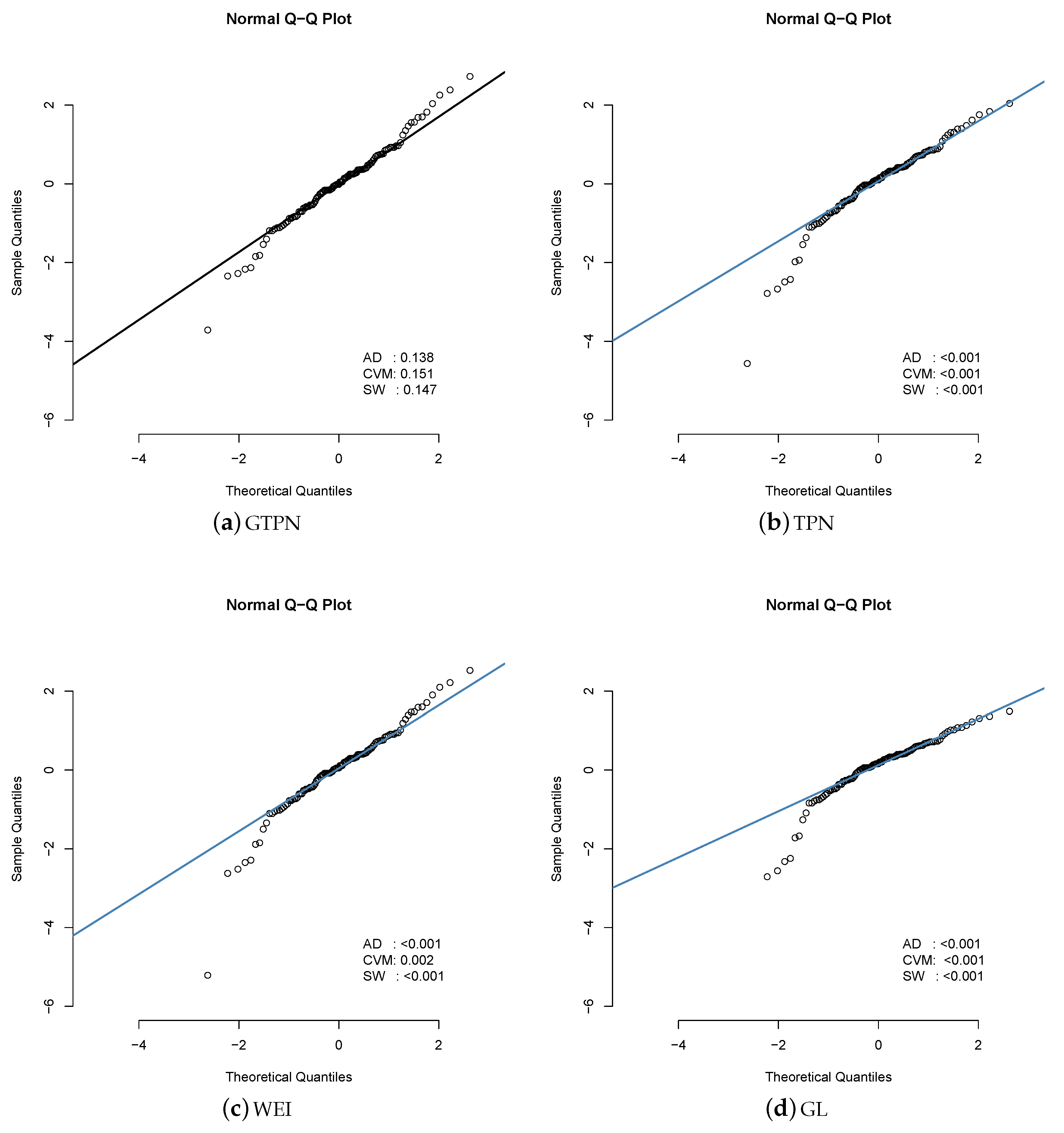
Initially, we calculate the estimators based on the centiles, naive, and moments of the GTPN distribution, which are ${\theta }_{cent}=(2.326,2.741,2.376)$, ${\theta }_{naive}=(3.557,0,1)$, and ${\theta }_{mom}=(3.075,1.572,3.203)$. We used these estimations as initial values in computing the ML estimators for the GTPN model. Results are presented in

Table 3. Estimation of the parameters and their standard errors (in parentheses) for the GTPN, TPN, WEI, and GL models for the data set. The AIC and BIC criteria are also included.

Estimated	GTPN	TPN	WEI	GL
$\sigma$	2.354(0.379)	0.720(0.047)	5.855(0.435)	-
$\lambda$	2.512(0.495)	4.842(0.333)	3.744(0.062)	4.093(0.539)
$\alpha$	2.227(0.401)	-	-	13.467(1.902)
$\gamma$	-	-	-	15.528(29.638)
AIC	238.43	254.63	251.74	308.67
BIC	246.67	260.12	257.23	316.90

. Note the high estimated standard error for the $\gamma$ parameter in the GL model. In addition, note that, based on the AIC criteria and BIC criteria [22], the GTPN model is preferred (among the fitted models) for this data set. Figure 6 shows the estimated density for each model in this data set, where the GTPN model appears to provide a better fit. Finally, Figure 7 also presents the qq-plot for the QR in the same models and the $p-values$ for the three normality tests discussed in Section 4.2. Results suggest that the GTPN model is an appropriate model for this data set while the rest of models are not.

6.2. Application 2

The data set to be investigated was taken from Nierenberg et al. [23], and is related to a study on plasma retinol and betacarotene levels from a sample of $n=315$ subjects. More specifically, the response variable observed is grams of cholesterol consumed per day. Descriptive statistics for the variable are provided in

Table 4. Descriptive statistics for the cholesterol data set.

Data Set	n	$\overline{\mathit{X}}$	${\mathit{S}}^{\mathbf{2}}$	$\sqrt{{\mathit{b}}_{\mathbf{1}}}$	${\mathit{b}}_{\mathbf{2}}$
Heights measured	315	242.46	17421.79	1.47	6.34

.

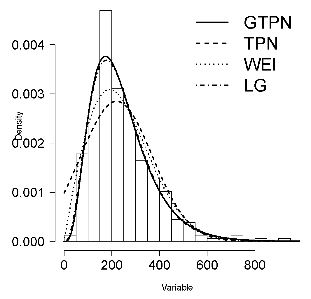
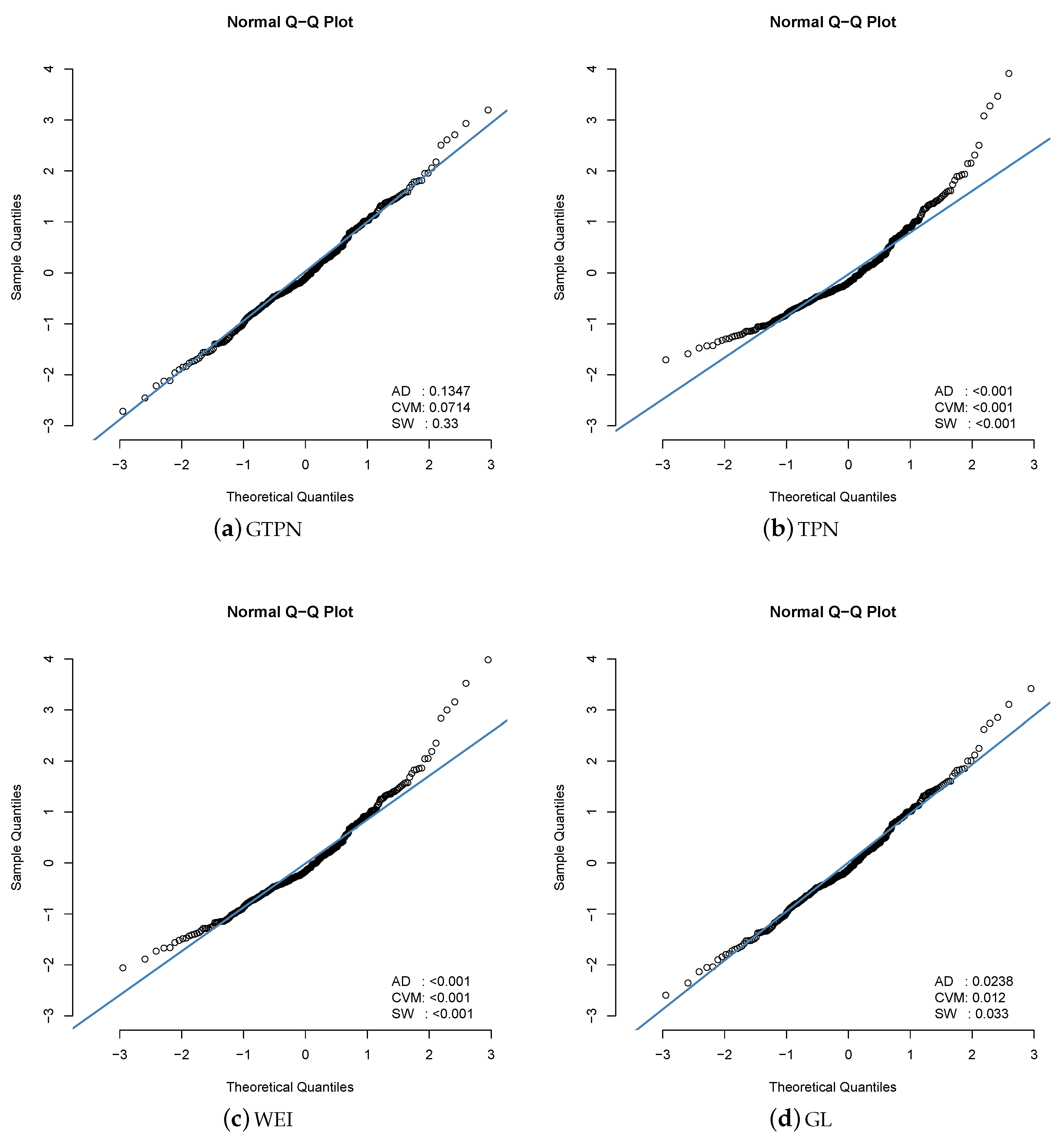
Initially, we calculate the estimators based on the centiles, naive, and moments of the GTPN distribution, which are ${\theta }_{cent}=(2.326,2.741,2.376)$, ${\theta }_{naive}=(275.960,0,1)$, and ${\theta }_{mom}=(0.003,-86.024,1.854)$. We used these estimations as initial values in computing the ML estimators for the GTPN model.

Table 5. Estimated parameters and their standard errors (in parentheses) for the GTPN, TPN, WEI, and GL models for the $cholesterol$ data set. The AIC and BIC criteria are also presented.

Estimated	GTPN	TPN	WEI	GL
$\sigma$	0.040(0.027)	151.106(8.734)	1.964(0.080)	-
$\lambda$	7.888(0.459)	1.455(0.138)	274.717(8.353)	0.016(0.001)
$\alpha$	0.240(0.013)	-	-	2.831(0.293)
$\gamma$	-	-	-	2.067(6.720)
AIC	3874.92	3943.25	3905.68	3879.07
BIC	3886.17	3950.75	3913.18	3890.42

summarizes the fit for this data set. As in last application, we noted the high estimated standard error for the $\gamma$ parameter in the GL model. Again, based on the AIC criteria and BIC criteria, the preferred model is the GTPN. Figure 8 shows the estimated density for each model in the cholesterol data set. The GTPN model appears to provide a better fit. For this data set, we also present the hypothesis tests for the three particular models of the GTPN distribution discussed in Section 4.1. Specifically, for $H_0^{\left(1\right)}:\alpha =1$ versus $H_1^{\left(1\right)}:\alpha \ne 1$ we obtained $p-values<0.0001$, $0.0157$, and $<0.0001$ for the SLR, SR, and ST tests, respectively. Therefore, with a significance of 5% we preferred the GTPN over the TPN model. For $H_0^{\left(2\right)}:\lambda =0$ versus $H_1^{\left(2\right)}:\lambda \ne 0$ we obtained $p-values<0.0001$, $0.0008$ and $<0.0001$ for the SLR, SR and ST tests, respectively. Hence, with a significance of 5% we preferred the GTPN over the GHN model. Finally, $H_0^{\left(3\right)}:(\alpha ,\lambda )=(1,0)$ versus $H_1^{\left(3\right)}:(\alpha ,\lambda )\ne (1,0)$ we obtained $p-values<0.0001$ for the three tests. Therefore, with a significance of 5% we preferred the GTPN over the HN model. Finally, Figure 9 also presents the qq-plot for the QR in the fitted models and the $p-values$ for the three normality tests. Results suggest that the GTPN model is appropriate for this data set while the rest of the models are not.

7. Conclusions

In this work we introduce a new distribution for positive data named the GTPN model. This new distribution includes as particular cases three models well-known in the literature: the TPN, GHN, and HN models. The basic properties of the model and ML estimation were studied. We performed a simulation study in finite samples and two real data applications, showing the good performance of the model compared with other usual models in the literature.

References

- Pewsey, A. Large-sample inference for the general half-normal distribution. Commun. Stat. Theory Methods 2002, 31, 1045–1054. [Google Scholar] [CrossRef]
- Pewsey, A. Improved likelihood based inference for the general half-normal distribution. Commun. Stat. Theory Methods 2004, 33, 197–204. [Google Scholar] [CrossRef]
- Wiper, M.P.; Girón, F.J.; Pewsey, A. Objective Bayesian inference for the half-normal and half-t distributions. Commun. Stat. Theory Methods 2008, 37, 3165–3185. [Google Scholar] [CrossRef]
- Khan, M.A.; Islam, H.N. Bayesian analysis of system availability with half-normal life time. Math. Sci. 2012, 9, 203–209. [Google Scholar] [CrossRef]
- Moral, R.A.; Hinde, J.; Demétrio, C.G.B. Half-normal plots and overdispersed models in R: The hnp package. J. Stat. Softw. 2017, 81, 1–23. [Google Scholar] [CrossRef]
- Azzalini, A. A class of distributions which includes the normal ones. Scand. J. Stat. 1985, 12, 171–178. [Google Scholar]
- Azzalini, A. Further results on a class of distributions which includes the normal ones. Statistics 1986, 12, 199–208. [Google Scholar]
- Henze, N. A probabilistic representation of the skew-normal distribution. Scand. J. Stat. 1986, 13, 271–275. [Google Scholar]
- Cooray, K.; Ananda, M.M.A. A generalization of the half-normal distribution with applications to lifetime data. Commun. Stat. Theory Methods 2008, 10, 195–224. [Google Scholar] [CrossRef]
- Olmos, N.M.; Varela, H.; Gómez, H.W.; Bolfarine, H. An extension of the half-normal distribution. Stat. Pap. 2012, 53, 875–886. [Google Scholar] [CrossRef]
- Cordeiro, G.M.; Pescim, R.R.; Ortega, E.M.M. The Kumaraswamy generalized half-normal distribution for skewed positive data. J. Data Sci. 2012, 10, 195–224. [Google Scholar]
- Gómez, Y.M.; Bolfarine, H. Likelihood-based inference for power half-normal distribution. J. Stat. Theory Appl. 2015, 14, 383–398. [Google Scholar] [CrossRef]
- Gómez, H.J.; Olmos, N.M.; Varela, H.; Bolfarine, H. Inference for a truncated positive normal distribution. Appl. Math. J. Chin. Univ. 2015, 33, 163–176. [Google Scholar] [CrossRef]
- Bonferroni, C.E. Elementi di Statistica Generale; Libreria Seber: Firenze, Italy, 1930. [Google Scholar]
- Arcagnia, A.; Porrob, F. The Graphical Representation of Inequality. Rev. Colomb. Estad. 2014, 37, 419–436. [Google Scholar] [CrossRef] [Green Version]
- Shannon, C.E. A Mathematical Theory of Communication. Bell Syst. Tech. J. 1948, 27, 379–423. [Google Scholar] [CrossRef] [Green Version]
- Akaike, H. A new look at the statistical model identification. IEEE Trans. Auto. Contr. 1974, 19, 716–723. [Google Scholar] [CrossRef]
- Dunn, P.K.; Smyth, G.K. Randomized Quantile Residuals. J. Comput. Graph. Stat. 1996, 5, 236–244. [Google Scholar]
- Yazici, B.; Yocalan, S. A comparison of various tests of normality. J. Stat. Comput. Simul. 2007, 77, 175–183. [Google Scholar] [CrossRef]
- Zakerzadeh, H.; Dolati, A. Generalized Lindley Distribution. J. Math. Ext. 2009, 3, 1–17. [Google Scholar]
- Laslett, G.M. Kriging and Splines: An Empirical Comparison of Their Predictive Performance in Some Applications. J. Am. Stat. Assoc. 1994, 89, 391–400. [Google Scholar] [CrossRef]
- Schwarz, G. Estimating the dimension of a model. Ann. Stat. 1978, 6, 461–464. [Google Scholar] [CrossRef]
- Nierenberg, D.W.; Stukel, T.A.; Baron, J.A.; Dain, B.J.; Greenberg, E.R. Determinants of plasma levels of beta-carotene and retinol. Am. J. Epidemiol. 1989, 130, 511–521. [Google Scholar] [CrossRef] [PubMed]
Figure 1.
Particular cases for the GTPN distribution.
Figure 2.
Density and hazard functions for the model with different combinations of and .
Figure 3.
Plots of the (a) expectation, (b) variance, (c) skewness and (d) kurtosis for for as a function of . In (d), the dashed line represents the kurtosis of the normal distribution.
Figure 4.
Bonferroni curve for the generalized truncation positive normal (GTPN) model.
Figure 5.
Entropy for the model.
Figure 6.
Fit of the distributions for the Laslett data set.
Figure 7.
QR for the fitted models in the Laslett data set. The for the Anderson–Darling (AD), Cramer-Von-Mises (CVM) and Shapiro–Wilks (SW) normality tests are also presented to check if the RQ came from the standard normal distribution.
Figure 8.
Fit of the distributions for the cholesterol data set.
Figure 9.
RQ for the fitted models in the cholesterol data set. The for the AD, CVM, and SW normality tests are also presented to check if the QR came from the standard normal distribution.