Design, Analysis, and Comparison of Control Strategies for an Industrial Robotic Arm Driven by a Multi-Level Inverter


Department of Electrical Engineering, Universidad de Santiago de Chile, Avenida Ecuador 3519, Estación Central, Santiago 9170124, Chile
*
Author to whom correspondence should be addressed.
Symmetry 2021, 13(1), 86; https://doi.org/10.3390/sym13010086
Submission received: 13 December 2020
/
Revised: 1 January 2021
/
Accepted: 3 January 2021
/
Published: 6 January 2021
(This article belongs to the Section Computer)
Abstract
:In this article, we present the design and implementation of different control strategies for the position of a 2-Degree-of-Freedom (DoF) robotic arm, namely gain scheduling per trenches, gain scheduling by interpolation, adaptive control, and fuzzy logic. The first link of this robot is driven by an Alternating Current Brushless Permanent Magnet Motor (ACBPMM) through a three-phase multi-level inverter with 27 levels of voltage per phase. Thanks to the topologies offered by ACBPMMs and to the multi-level inverter, high commutation frequencies are reduced, as observed in the computer simulations. Additionally, to determine which proposed control strategies are the most suitable for an ACBPMM connected to a multi-level inverter, a comparative study on the performance of the controllers implemented for this robot is conducted.
1. Introduction
For decades, the robotics field has experienced widespread acceptance and growth. In particular, polymorphic robots are generally used in the industry, which has generated the need of constantly creating industrial robots with more power, speed, and precision for a wide variety of tasks, including mining [1,2,3,4,5,6,7,8].
Nowadays, Direct Current (DC) servomotors are widely used for building up robotic systems with several degrees of freedom and varied morphologies due to their movement accuracy and low cost. Physically, DC servomotors are constituted by a DC motor, a gear train for spin speed reduction and torque increase in the drive axle (spindle), a potentiometer connected to this output shaft for obtaining position, and a feedback control circuit that converts an input Pulse-Width Modulation (PWM) signal into voltage by comparing it with the feedback position, and then amplifying it to activate an H-Bridge that produces spin with a determined speed. However, because of their commutators, the DC motors of polymorphic robots need costly periodical maintenance. In addition, the faults in the actuators of these robots can cause danger for operators, difficulties for users, unplanned shutdowns, and economic losses, among other consequences. Therefore, as a solution for this problem, studies have been conducted to actuate the links of polymorphic robots using AC machines [9,10,11,12,13,14,15,16,17,18].
Initially, the use of AC machines—including Alternating Current Brushless Permanent Magnet Motors (ACBPMMs)—was limited to basic operations for moving loads at a constant speed. Over time, with the advent of frequency converters and soft starters, the ignition of these motors saw nominal current and work speed reduced. Currently, these devices have a strong presence in the industrial and mining sectors. Over time, these electronic devices evolved, and new techniques emerged, such as vector control, which allows for starting an AC machine with an initial load [19,20,21].
However, despite the technological development of power electronics in the field of AC machines, these motors were not competitive against DC machines in the robotics field, especially in position control, although the latter have lower performance than AC machines and require more maintenance. In fact, the only implementation alternative for AC machines was conducted through a synchronous brushless motor controlled by a two-level inverter with pulse-width modulation. However, when using larger motors, this modulation used to cause problems as it required expensive semi-conductors to perform commutations, generating overheating and loss of efficiency of the circuits associated to the AC machines, as well as harmonics at the entrance of the inverter, which produce high levels of dv/dt and high commutation frequencies that hinder the service life of the AC machines. These difficulties led to the development of multi-level inverters in the mid-80s. The topologies of these devices have different AC-output voltages, and the number of levels is the same as the number of DC-input voltage sources. The main topologies used in the multi-level inverters are the following [22,23,24,25,26,27,28,29,30,31,32,33]:
- (1)
- Two-Level Inverter
This topology is the most basic but widespread in the industry because of its simple structure, application, and control. In this topology, only two electronic switches are required, such as Metal-Oxide-Semiconductor Field-Effect Transistors (MOSFETs), Insulated Gate Bipolar Transistors (IGBTs), and Gate Turn-Off Thyristors (GTOs), among others, which should be used based on working frequency and voltage. However, for high voltage levels, switches in series should be employed. The modulation techniques most used in this type of topologies are Sinusoidal PWM (SPWM), PWM with third harmonic injection, Space-Vector Modulation (SVM), and Selective Harmonic Elimination (SHE).
- (2)
- Inverter coupled by Diodes and their Derivations
The following configurations derive from this topology based on diode and capacitors arrays to produce different voltages:
- Neutral-Point-Clamped (NPC), which delivers three levels of voltage from different DC voltage sources, or from a single one that is divided with capacitors in series.
- Diode/Capacitor Clamped (DCC), which is a modification of the NPC category as it includes an additional capacitor to reduce the voltage peaks in the switches during commutation.
- New Diode Clamped (NDC), which is a modification of the NPC category as it includes additional diodes that block a same voltage in series.
- (3)
- Flying-Capacitor Inverter
In this topology, a large number of flying capacitors—located between the switches—is required to separate the input voltage source. To generate three voltage levels, 3 capacitors and 4 switches are required, while 10 capacitors and 8 switches are necessary to produce 5 levels of voltage. Therefore, voltage increase is proportional to the number of devices required. This topology allows for both eliminating the diodes required by the topologies above and arranging several combinations to generate the same voltage. In this way, switches can work alternately, avoiding overheating and extending their service life. Nevertheless, this topology has the drawback of requiring a large number of capacitors, which rises implementation costs.
- (4)
- Cascaded Full-Bridge Inverter
The following configurations derive from the cascade array in this topology:
- Inverter with cascaded symmetrical monophase bridges that uses a monophasic H-bridge to deliver 3 levels of output voltage. However, a cascaded connection of 2 H-bridges enables 5 output voltage levels. By increasing the number of cascaded H-bridges, the number of output voltage levels can be increased with a small quantity of components and without the need of clamping diodes or flying capacitors.
- Cascaded hybrid asymmetrical inverter that has the same topology described above but with only a fraction of the voltage level that feeds each H-bridge, allowing for a 7-level increase in output voltage.
- Inverters coupled by converters in which only one DC voltage source for each H bridge is required, reducing the possibilities of short circuits during switch commutation. Additionally, the turns ratio of the converters allows for generating different voltage levels. Although this configuration has the advantage of employing only one voltage source, it exhibits the economic disadvantage of adding converters.
- Cascaded multi-level inverters used to work with high voltage and power levels. With this purpose, the cascaded H-bridge stages are replaced by flying capacitors or clamping diodes, thereby reducing the number of voltage sources isolated in the inverter input. For example, to generate 9 voltage levels, 2 converters with cascaded flying capacitors can be used so only two independent voltage sources are necessary, whereas the cascaded H-bridge configuration requires 4 independent voltage sources.
The use of these topologies allows for increasing the power of the inverters thanks to the incorporation of more voltage levels without the need of increasing current, reducing Joule losses, decreasing Total Harmonic Distortion (THD) due to the increase of voltage levels, reducing dv/dt variations between voltage levels, and extending the service life of the motor coiling, among other advantages. Nevertheless, the main disadvantage of these topologies when used in multi-level inverters lies in the increase in the number of voltage levels, which rises implementation costs due to the incorporation of switches, capacitors, and voltage sources to achieve the maximum desired voltage level and the number of steps necessary for this.
The control techniques of the multi-level inverters aim to minimize the harmonic content of output voltage in the inverter, regulate output amplitude and frequency, and balance the instant voltages of the capacitors when the topology requires so. Field-Oriented Control (FOC), or Vector Control (VC), is a Variable Frequency Drive (VFD) control technique in which the stator currents of a three-phase AC motor are identified as two orthogonal components that can be visualized with a vector. One component defines the magnetic flux of the motor, and the other its torque. FOC allows for obtaining almost instantaneous changes in torque on demand, and in essence it does this by jumping directly from one steady state condition to another, without any unwelcomed transient period of adjustment. FOC typically uses Proportional-Integral (PI) controllers where the current components are compared to reference values, rather than using PWM. This allows electric motors to operate smoothly over the full speed range and generate full torque at zero speed. Another benefit of FOC is that it can make the motor accelerate and decelerate fast, providing more accurate control in high performance motors. Nowadays, FOC is used to control AC synchronous and induction motors, and it is becoming increasingly attractive for lower performance applications due to its superiority in reducing motor size, as well as power consumption and its related costs [34,35,36,37,38]:
ACBPMMs have permanent magnets that rotate around a fixed armature, eliminating problems associated with connecting current to the moving armature. They are composed of a three-phase stator and a permanent magnet rotor. These components turn them into synchronous machines that require power electronics to control and optimize their operation. However, compared with conventional motors with brushes, their main advantages are the following [39,40,41]:
- (1)
- More power for the same size.
- (2)
- Wider speed range, as they do not have mechanical limitations.
- (3)
- More efficiency as they lose less heat.
- (4)
- Better performance.
- (5)
- Longer shelf life.
- (6)
- Better speed/motor torque ratio.
- (7)
- More heat dissipation.
- (8)
- Lower weight.
- (9)
- Less maintenance due to absence of wear.
- (10)
- Less electronic noise.
Additionally, AC machines, compared to DC motors, offer advantages such as controlled acceleration and adjustable speed and torques depending on the requirements. Conversely, faults in the DC motors of the links of a robot can cause many problems. As a solution, this work presents the design and implementation of different control strategies for the position of a 2- DoF robotic arm, namely gain scheduling per trenches, gain scheduling by interpolation, adaptive control, and fuzzy logic. The robot model to be developed includes the largest quantity of variables influencing link position, and does not only consider the physical variables weight, length, mass center, and inertia, but also the friction torque that includes the static, viscous, and Coulomb friction forces. All the above will be used in combination with the real parameters of a robotic arm, an AC motor, a DC motor, and a speed reducer to improve test reliability. To control the AC motor, a three-phase multi-level inverter with 27 levels of voltage per phase, like the one presented in Appendix A, will be considered. In addition, to determine which proposed control strategies are the most suitable for an ACBPMM connected to a multi-level inverter, a comparative study will be carried out on the performance of the controllers to be implemented for this robot.
2. Materials and Methods
In this work, the selection of an ACBPMM arm is the first problem to be solved in the actuation of the first link of a 2-DoF robot. In this case, a three-phase synchronous brushless motor was selected, whose parameters are shown in Table 1.
Then, a three-phase multi-level inverter with 27 levels of voltage per phase is considered to control this motor. This type of inverter has the advantage of reducing the high commutation frequency required by a permanent magnet motor, as shown in Figure 1.
To apply the different control strategies comprised by this work, the dynamic model of a 2-DoF robot, shown in Figure 2, was employed. This model is represented by Equation (1) and considers the torque of rotational dynamic friction that is generated from its gear system.
Equations (1) and (2) show the dynamic system of a 2-DoF robotic arm with rotational and prismatic joints, where is the mechanical torque of the arm in the first rotational joint, and is the force that the second link exerts over the first one.
where:
- : Torque applied to the first link (N · m).
- : Force applied to the second link (N).
- : Angular position of the first link (°).
- : Angular speed of the first link (°/s).
- : Angular acceleration of the first link (°/s2).
- : Longitudinal position of the second link (m).
- : First link mass (Kg).
- : Second link mass (Kg).
- : First link length (m).
- : Length from the first link origin to its center of mass (m).
- : Inertia moment of the first link (Kg · m2).
- : Inertia moment of the second link (Kg · m2).
- : Constant of the gravity exerted by the gravitational system in which the robot is (m/s2).
This dynamic model also comprises of the torque of rotational dynamic friction generated in the rotation axis. The friction torque is represented through a function that includes the effects of static, viscous and Coulomb frictions. Additionally, these functions allow for eliminating the numerical noise that computer simulations produce, which originates from rounding errors—due to the use of carriers in real arithmetic operations—and from truncation errors in numerical series in a finite number of terms. This is a linear function by segments, where for speed values (positive or negative) smaller than k, the friction function has a value of 0, while for higher k values, it grows linearly; the same is true for values below −k, as shown in detail in Equation (3).
where:
- : Friction torque in the arm rotation axis (N · m).
- : Slope of viscous friction for positive torque (N · m · s/rad).
- : Slope of viscous friction for negative torque (N · m · s/rad).
- : Coulomb’s friction constant for positive torque (N · m).
- : Coulomb’s friction constant for negative torque (N · m).
When considering the dynamic model presented in Equations (1) and (2), as well as the addition of the friction force from Equation (3), a model of the general dynamic system is obtained, as observed in Equation (4). This model also incorporates the gain produced by the gear system (r gain).
where:
- : Electromagnetic torque of the motor (N · m).
- : Inertia moment of the motor (Kg · m).
- : Angular speed of the motor (rad/s).
- : Viscous friction of the motor (N · m ·s/rad).
- : Gear ratio (times).
3. Implemented Control Strategies
When using a classic Proportional-Integral-Derivative (PID) controller in the actuator of the first link of the robotic arm, start and stability problems appear (from the resting position) when controlling for position. These problems worsen when the robotic arm is subject to disturbances, not only when it performs a movement, but when it reaches a position in stationary state. To solve this issue, a control strategy is designed and implemented, which modifies the PID controller parameters online at different stages of the process. The control system modifies the value of its control parameters depending on the angle at which the robotic arm is, as shown in Figure 3.
The incorporation of each control strategy for solving the problems in the robotic arm is described below. The first strategy implemented to substitute the classic PID controller is based on a closed loop and the modification of the controller parameters. After the dynamic performance of the model is analyzed, it is observed that the controller should be able to modify the PID parameters in the different work areas. To achieve this goal, the gain scheduling per trenches strategy is selected, as it offers such an advantage.
3.1. Gain Scheduling per Trenches
This strategy offers versatile control tailored to the requirements of each process, modifying such parameters according to the state of the process, and providing the additional advantage of operating autonomously at different points. Therefore, in this work, this controller seeks to compensate the dynamic change that the robotic arm experiences during motion due to the action of the gravitational force and its inertia. The dynamic change increases significantly when the robotic arm gains more speed. To tackle this issue across the different operation ranges of the robotic arm, gain scheduling per trenches allows for modifying the parameters of the controller, as shown in Table 2, where the value of the PID controller gains (Kp, Ki, and Kd, respectively) depends on the angular position of the robotic arm (θ1 = 15°; θ2 = 35°; θ3 = 60°, and θ4 = 75°).
From Table 2 and knowing the angular position of the robotic arm, the PID parameters of the controller that are used in the angular position controller are assigned, as observed in Figure 4.
This control strategy—whose results are shown and commented in the next section—stabilizes the robotic arm at different reference values and eliminates the stable status. However, the system is observed to be unstable when changing the reference position between one work area and another. Therefore, to avoid further divisions of the work areas, PID parameters are modified in the limit between trenches. The strategy used in this case, gain scheduling by interpolation, is presented below.
3.2. Gain Scheduling by Interpolation
In this second type of control, considering the angular position at which the robotic arm is located, the value of the controller gains corresponding to each border of the PID controller trenches is calculated through an interpolation polynomial, as shown in Figure 5. In this way, the coefficients of the PID controller parameters of the gain scheduling per trenches strategy are used, and a linear interpolation is applied to calculate the other parameters corresponding to the limits between trenches.
A control strategy for calculating its parameters according to system performance is presented below. In this case, adaptive control offers the advantage of being useful in processes with variable parameters.
3.3. Adaptive Control
Adaptive control is ideal for high performance applications in control systems with parameter uncertainty. It consists of adjusting the classic PID controller parameters as the real position of the manipulator robot varies, in order to reduce the rising time and overshoot of the system. However, the design of adaptive controllers requires solid knowledge of the structure of the system to be controlled.
In adaptive control, parameters are variables that can be adjusted online based on the system measurements. The adjustment mechanism used corresponds to the following equation:
where:
- : Parameter to be adjusted.
- : Positive constant that represents the adjustment mechanism.
- : Difference between desired and real positions (°).
- : Real position (°).
In this work, the calculation of each parameter of the Adaptive Controller of the robotic arm is conducted by approximating the real position value to the desired position value. In this way, the errors between angular positions, the derivatives of these errors and the accumulated error decrease progressively. Then, the calculation of each parameter is sent to the vector control that feeds the AC motor, which allows for the controlled movement of the robotic arm.
The fourth and last control strategy employed seeks to restrict the sudden rises in the speed of the robotic arm during its trajectory towards a desired angular position.
3.4. Fuzzy Logic
This strategy is classified as smart control because, in addition to conducting mathematical calculations for optimizing a process, it also has rules and constraints for them. Specifically, it attempts to determine in a logical way how to achieve the control objectives in the best possible way, departing from a knowledge base provided by a human operator. Nevertheless, without a knowledge base, developing a fuzzy controller that works properly is not possible. Fuzzy logic is used in complex systems and in systems controlled by human experts, among others. In addition, it enables the assessment in real time of a large quantity of variables with pre-established rules, which allows for applying the knowledge acquired by using some of the strategies above. Fuzzy logic is used in complex systems, and in systems controlled by human experts. In addition, it makes it possible to assess in real time a large number of variables with pre-set rules, which enables the application of the knowledge acquired from the previously reviewed strategies.
The operation of fuzzy logic is based on extending the two-value binary logic (ON/OFF, 0 or 1) to a continuous range from 0 to 1 (∀ number between [0,1] ∈ 𝕽), where initially the input value or values are analyzed in the membership functions, whether Gaussian, triangular, trapezoidal, etc., by assigning a value within the fuzzy set A ∈ S defined by μ A: S → [0,1], (A = ).
Subsequently, the output variable or variables are calculated based on the input ones and according to the set of rules defined by the controller.
Inference engines work primarily in one of two modes, either in special rules or facts: forward chaining and backward chaining.
This work employs the “fuzzy” toolbox from MatLab® as a base controller taking error and the error derivative as input values. The controller is configured to work with the two input variables above and the output variable, which is the action sent to the multi-level inverter.
4. Computer Simulations and Synthesis of Results
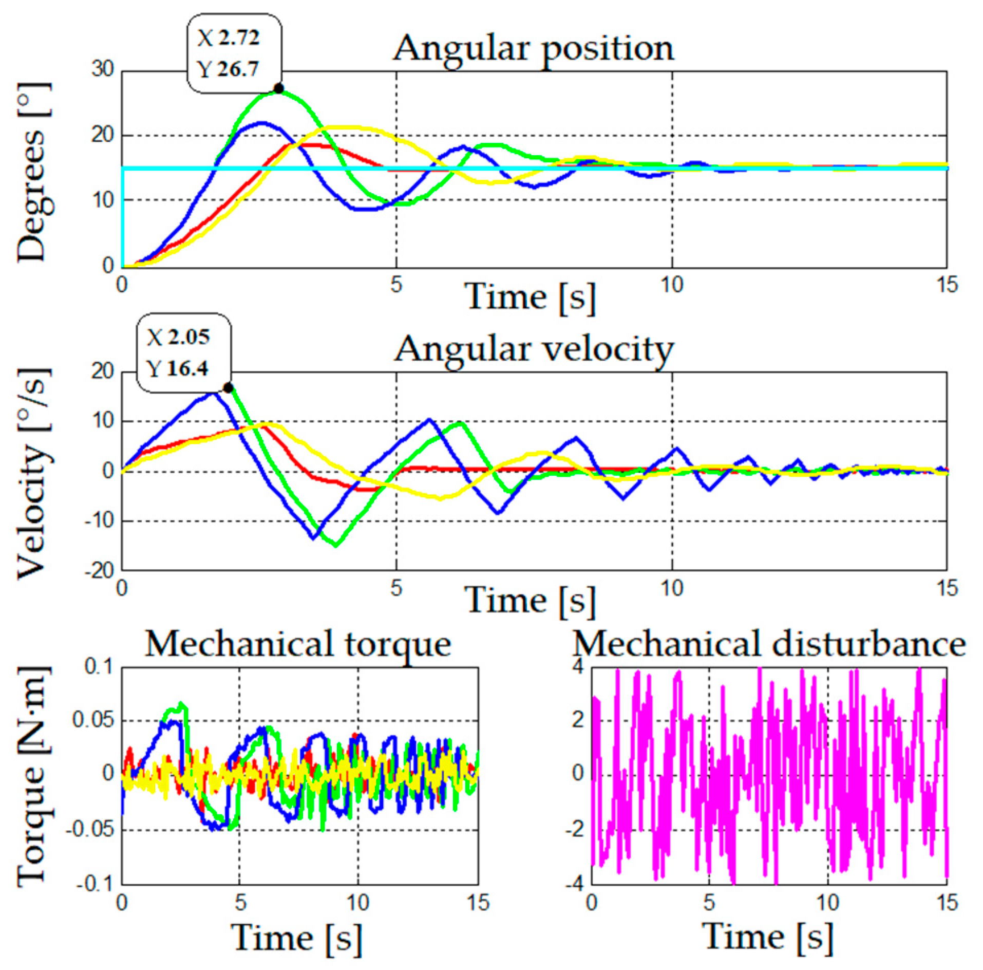
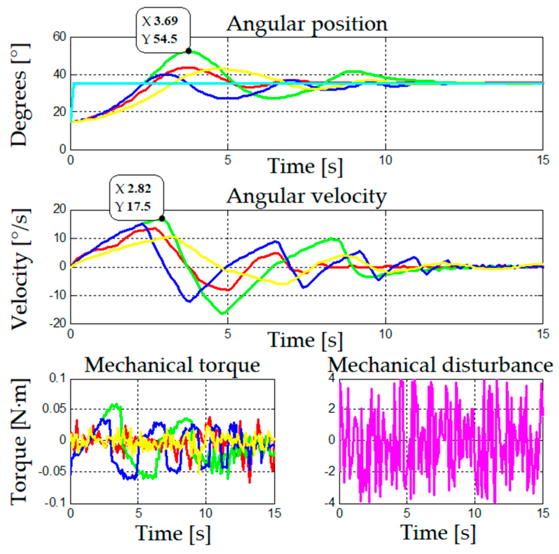
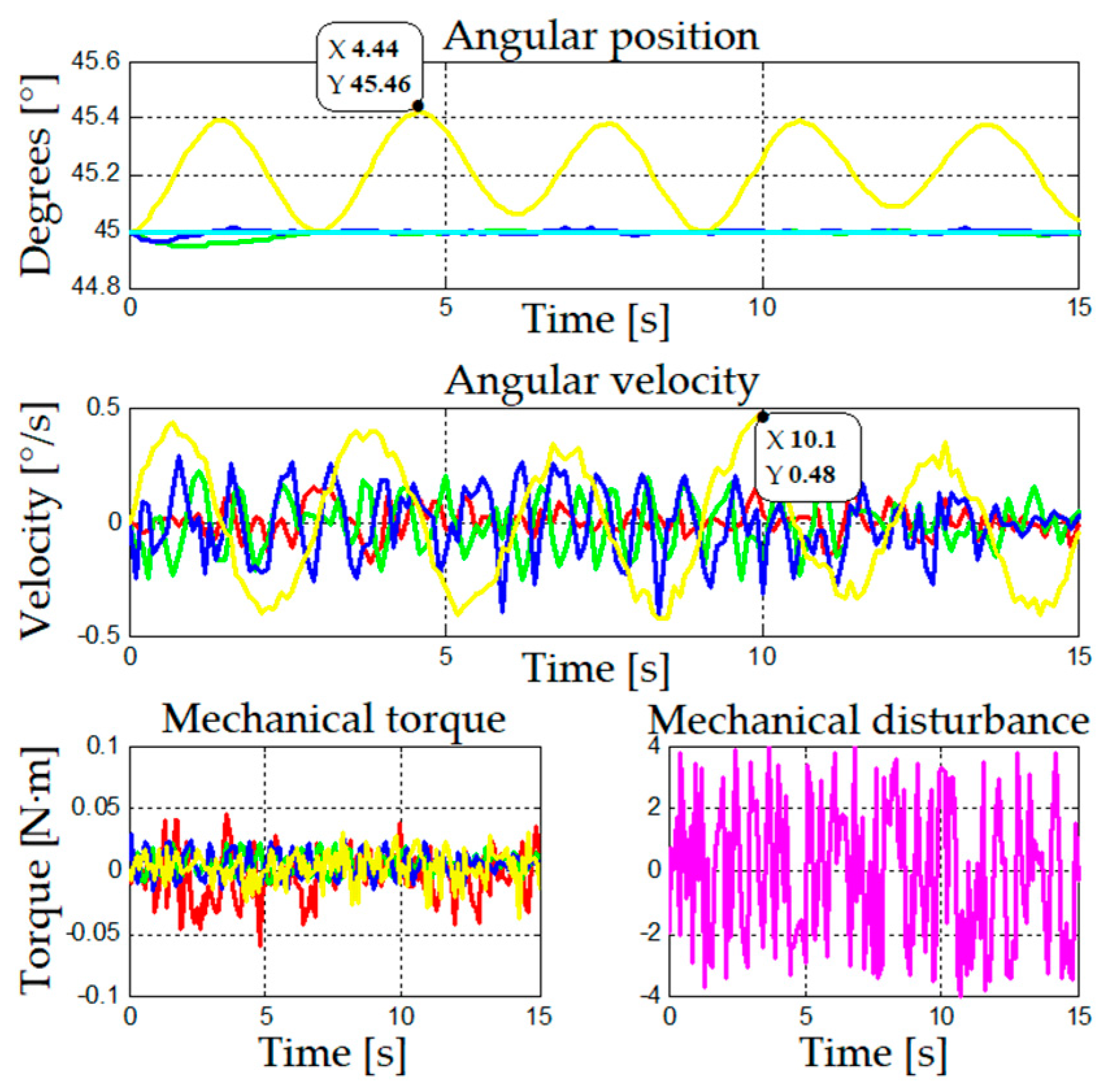
The results of the comparison between the four control strategies proposed for different movements of the robotic arm, graphing its position, speed, mechanical torque, and disturbance to which is subject are presented below. Each strategy is marked as follows:

4.1. Analysis of Control Strategies Applied to the First Link of the Robotic Arm
In Figure 6, the four proposed methods are observed to have similar performances, with an initial overshoot at 18° when using gain scheduling by interpolation compared to the other methods, which had overshoots between 3° and 7°. All strategies presented similar times to achieve a stable state.
In Figure 7, differences between strategies are slightly more pronounced, and each strategy exhibits advantages and disadvantages compared to the others. Gain scheduling per trenches shows low initial overshoot and is the strategy that reaches the stable state the fastest, while gain scheduling by interpolation is faster than the other three strategies but has a higher initial overshoot. On its part, adaptive control presents fast acceleration and lower initial overshoot but also difficulties to achieve the stable state, and fuzzy logic is the slowest but most stable strategy in this regard.
When working in higher areas, as observed in Figure 8, the four control strategies present difficulties. Gain scheduling methods show overshoot and instability in the stable state; adaptive control does not have considerable overshoot but fails to control position in the stable state, and fuzzy logic presents a behavior similar to the previous areas with overshoot and stability when reaching the reference value.
Figure 9 shows the behavior of the four control strategies when the stability of a fixed position is analyzed. When the desired position is in the lower areas (20°), the gain scheduling strategies present lower overshoot than adaptive control. Instead, the latter exhibits better behavior for higher work areas of the robotic arm. For these three strategies there is not visible difference in behavior, as they have an oscillation of ±0.005°, whereas fuzzy logic has the highest oscillation compared the other strategies. However, this is still a small value with an error below 0.5°.
The analysis of error indexes in Figure 10 shows the performance of the four control strategies when these are in a stable state, through the Index of Agreement (IA), Residual Mean Square (RMS), and Residual Standard Deviation (RSD). Initially, a good behavior is observed, as the results are within the reference values considered acceptable.
The control strategy gain scheduling by interpolation does not show good performance for the lower work areas when the system requires less force, as it is working in a more vertical zone, where gravity does not have much of an impact. This strategy exhibits a better behavior in areas where the motor is subject to higher work pressure but, in general, the system keeps the desired position after achieving the stable state.
The behavior of the two control strategies based on gain scheduling is similar under the same work conditions. A slightly better performance is observed when the controller parameters are adjusted by gain scheduling per trenches; in this case, the system is more sensitive (and preemptive) when reaching the reference value and has a slow reduction of speed such that overshoot is lower.
Considering a stability analysis of the controllers, the four control strategies showed good performance, with an error of ±0.2°, which is a success considering that the classic PID controller was not even able to stabilize itself and therefore would not be able to control the movement of the robotic arm until it reached a desired position. If one of the four control strategies should be chosen to be implemented in the robotic arm, it would be adaptive control, as it presents better performance than the others.
It must be noted that when the robotic arm works in the middle area (between 30° and 60°), the control strategies by gain scheduling encounter difficulties. This is due to the sudden addition of the gravity force, which increases in a factor of 0.5 (for 30°), and 0.86 (for 60°) in the sine function of Equation (1). Conversely, adaptive control does not experience problems in this critical area. Instead, it adapts to the sudden variation of the manipulator robot caused by gravity. This indicates that the robotic arm will perform better with this strategy, considering the environment where the arm will operate.
The fuzzy logic strategy presents a stable behavior in terms of overshoot, stability, and behavior across work areas. Additionally, this strategy has the most stable speed, reason why its implementation was considered.
The error analysis shows that the best robotic arm performance is achieved with adaptive control for all the tests conducted. Therefore, this is the control strategy proposed as the most suitable for an ACBPMM connected to a multi-level inverter.
4.2. Analysis of Control Strategies Applied in the Two Links of the Robotic Arm
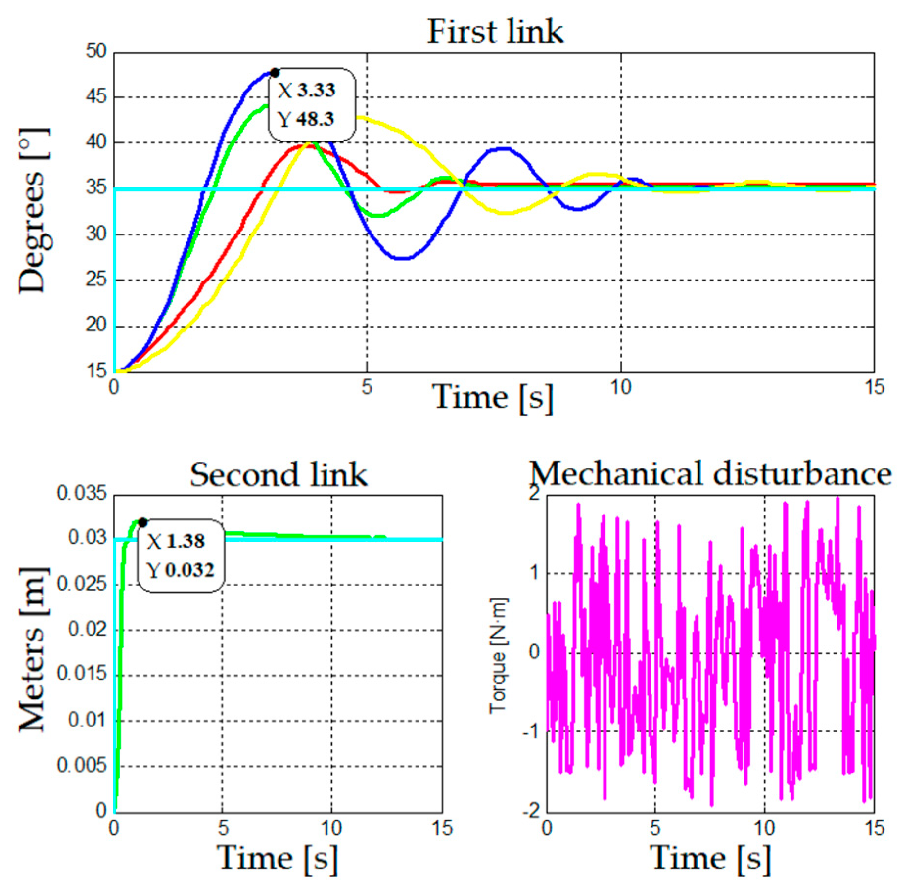
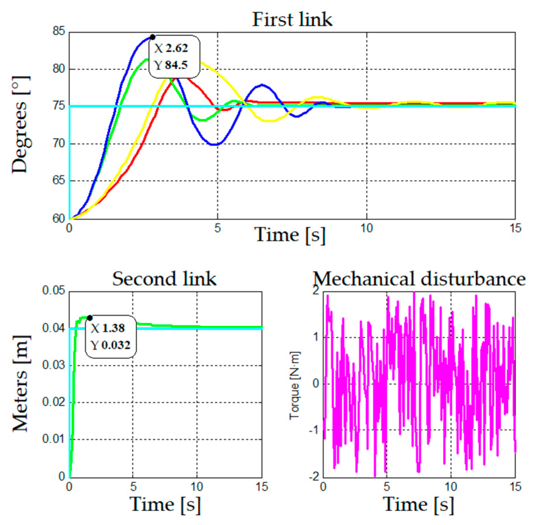
The proposed control strategies will be implemented in the 2-DoF robotic arm. The performance of the two links (rotational and prismatic) is compared when using the different control strategies. It may be seen in Figure 11 that adaptive control has stabilization difficulties: the system becomes instable for the calculation of the PID parameters when adding the second prismatic link and presents oscillation and delay to reach the stable state. The gain scheduling strategies behave better, especially gain scheduling by trenches, while the fuzzy logic controller also presents initial overshoot.
A similar behavior is observed in Figure 12, where gain scheduling per trenches performs the best, while adaptive control has more initial overshoot than the other strategies.
In general, gain scheduling per trenches has high initial overshoot, and adaptive control presents stability problems, whereas the other two strategies have stable performances in terms of overshoot and stability. Nevertheless, in the following work areas, gain scheduling (per trenches or by interpolation) presents better performance, since it is the most stable component of the dynamic model weight, as observed in Figure 13. Conversely, fuzzy logic and adaptive control are too sudden to calculate parameters. Adaptive control, particularly, requires increasing proportional and integrative gains to correct the initial error, which leads to an initial overshoot and oscillation during the first seconds. The same is true for fuzzy logic; in this case, the corrective action after reaching the desired value is too slow, and the change in the rotation direction is not able to overcome the rotation inertia of the robotic arm.
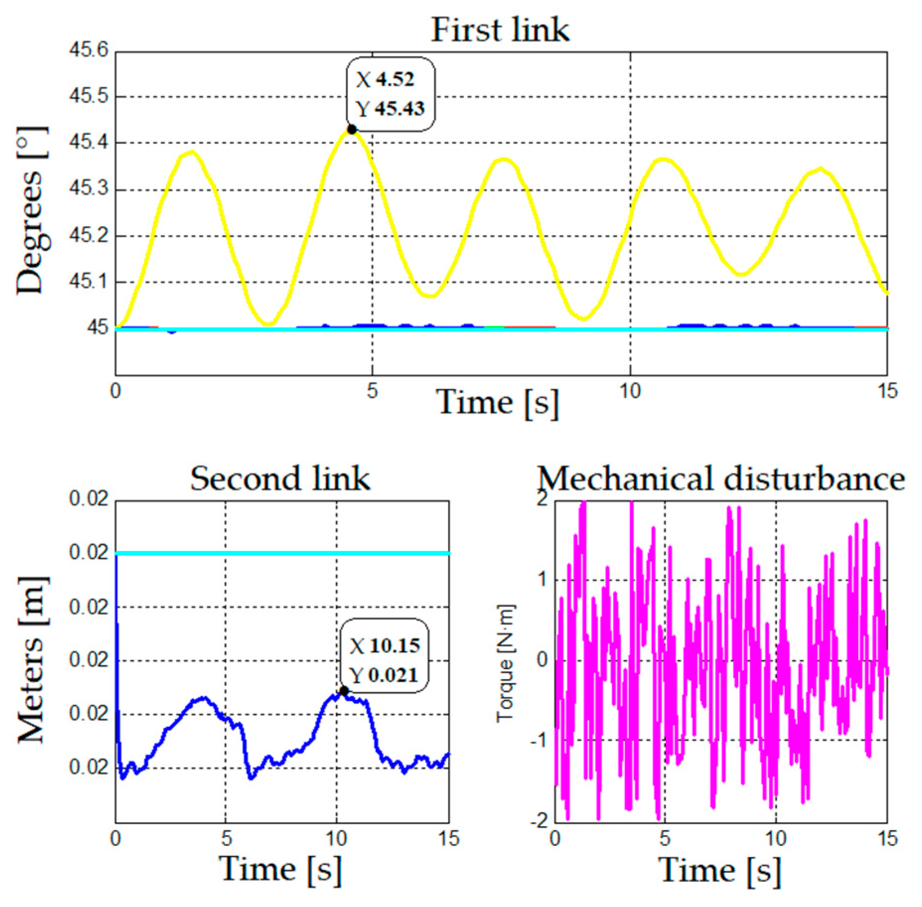
When analyzing the strategies for stability, all of them are observed to be satisfactory, as shown in Figure 14. However, all of them oscillate between ±0.006° from the reference position, except from fuzzy logic, which takes a maximum error of 0.4°.
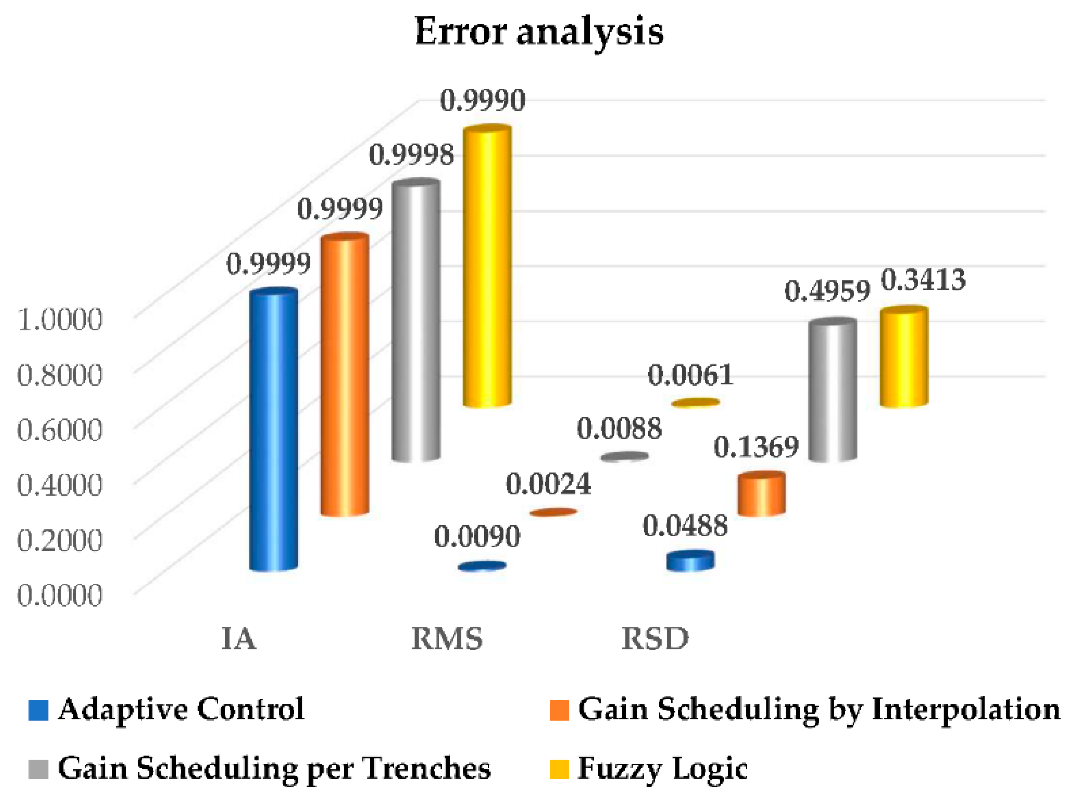
After the calculation of the error indexes of the first link when stability is reached, all the control strategies used exhibit a good behavior in all indicators, as shown in Figure 15. IA has a value close to 1, while RMS and RSD have values close to 0. Adaptive control performs better than the other two strategies proposed.
Performance differences are observed when using the rotational joint under different control strategies in a 2-DoF robotic arm. In this case, the variation of the second prismatic link implied a variation in the weight of the robotic arm. This translates into instability for the system in areas where the weight component is more significant.
From the above, the control strategy gain scheduling per trenches presents better behavior in areas where the weight component is more stable, i.e., in areas below 20° and above 70° it performed well, but the system was quite instable in areas where weight experienced more significant variations.
The second strategy, gain scheduling by interpolation, is the most stable of the control strategies reviewed. With this strategy, regardless of the work area, the system remained stable because of the linear adjustment between PID parameters, which prevents parameters from varying abruptly.
The third strategy, adaptive control, presents difficulties due to a sudden change in the calculation of the PID parameters. When the second link is triggered, the adaptive control system becomes too sensitive to this movement due to the inertia of the robotic arm. This causes an increase in the P parameter that leads to more overshoot, which in turn, generates a decrease in the D parameter, making the movement of the robotic arm slower.
Fuzzy logic presents a behavior similar to the previous test, being stable in all work areas but with a small initial overshoot to achieve stability.
Confronted with the dynamic changes in the rotational link of the robotic arm, which becomes more accentuated due to the prismatic link, the control strategy gain scheduling by interpolation performs better than the other control strategies.
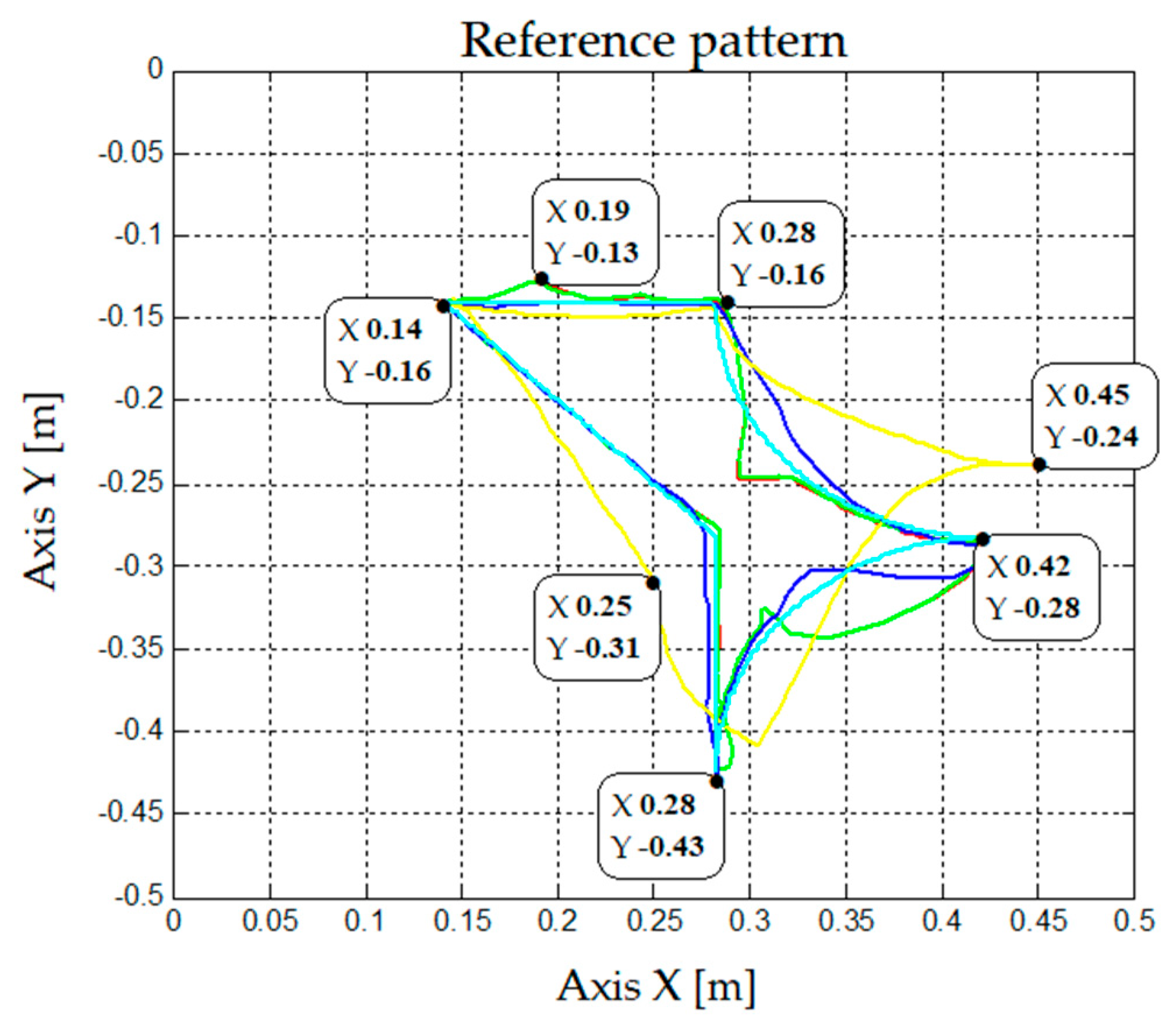
4.3. Analysis of the Control Strategies Applied in the Pattern Tracking of the Robotic Arm
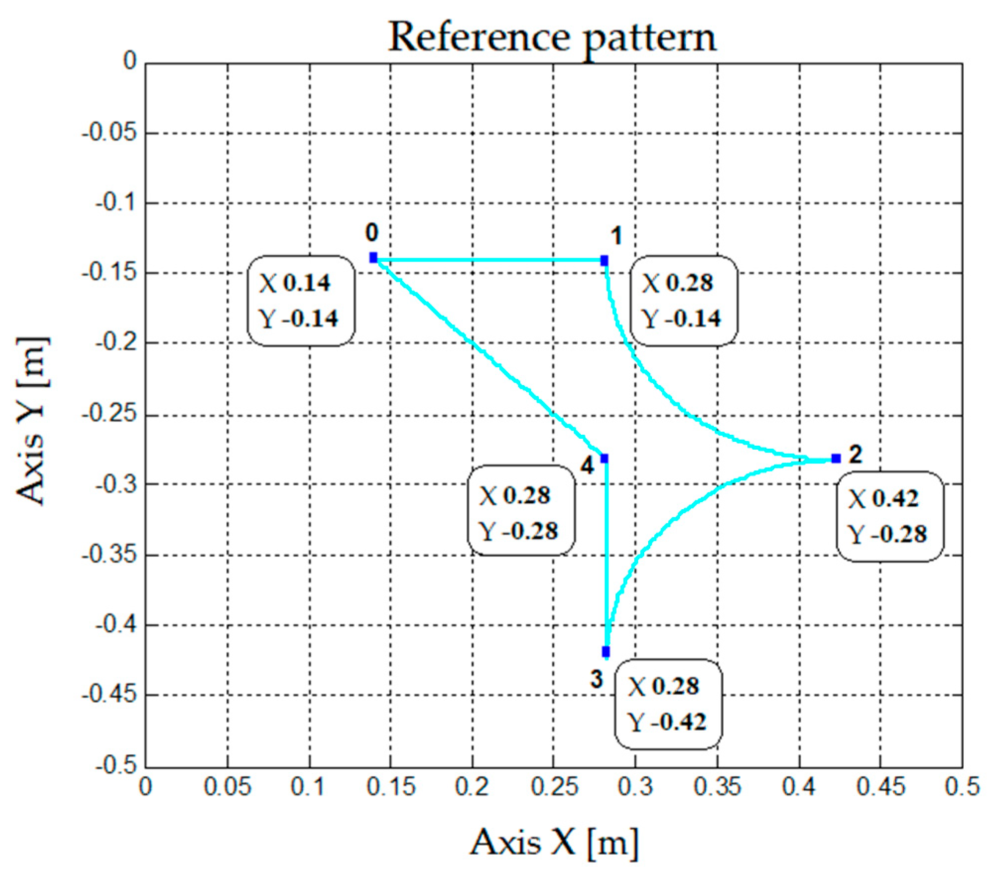
In this section, the control strategies will be compared when the robotic arm performs different work patterns, i.e., specific routes across Cartesian X and Y axes. First, the pattern to be followed will be presented; then, the strategies used will be compared when following this pattern, and finally, the performance of each link and the disturbance to which the rotational link is subject will be shown. The pattern on which the control strategies will be applied is based on straight, diagonal, and curve lines on the Cartesian plane, as shown in Figure 16. The route follows the numerical sequence from 0 to 4 until returning to the start 0. This pattern imposes more variations in the references on the Cartesian axes, and in the reference values of each link compared to the previous patterns.
In this pattern, the differences between the control strategies are evident. Adaptive control stands out over the two gain scheduling strategies, as seen in Figure 17. This is clear in Figure 18 since, between seconds 2 and 8, where the reference of the first rotational link are quadratic functions, the adaptive control strategy performs better than the other two strategies.
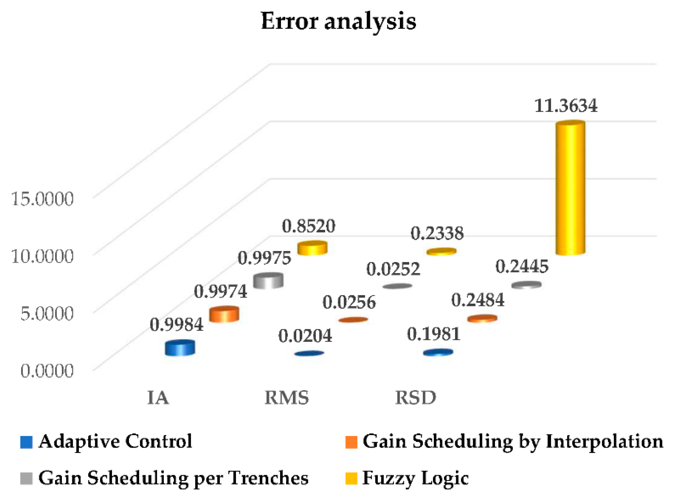
Through the calculations of error indexes from the first link at all times—differently from the previous calculations, which were conducted when reaching the stable state—all control strategies are observed to have a good performance according to the indicators, as shown in Figure 19. IA has a value close to 1 for the three control strategies, and the RMS index has a value close to 0. However, big differences emerge with the RSD index, as it yields significant error for the fuzzy logic strategy, which has different values and indicates a better performance from adaptive control.
Gain scheduling and adaptive control perform satisfactorily for the reference pattern.
Adaptive control, gain scheduling by interpolation, and gain scheduling per trenches are similar in their behavior when following the reference pattern, but fuzzy logic shows a different behavior. Nevertheless, when the robotic arm moves continuously on one axis, either constantly on the X axis or varying linearly on the Y axis, or vice versa, the two gain scheduling strategies have difficulties to remove error.
5. Conclusions
In this work, the design and implementation of different control strategies for the position of a 2-DoF robotic arm was presented. The robot model developed comprises of the largest quantity of variables influencing link position, and does not only consider the physical variables weight, length, mass center, and inertia, but also the friction torque that includes the static, viscous, and Coulomb friction forces. All the above was used in combination with the real parameters of a robotic arm, an AC servomotor, a DC motor, and a speed reducer, which made the tests more reliable. To control the AC motor (three-phase synchronous brushless motor), a three-phase multi-level inverter with 27 levels of voltage per phase was considered.
Regarding the control strategies studies, first a position control system that modified the PID controller parameters online—depending on the angle at which the robotic arm is—was designed and implemented. Subsequently, gain scheduling per trenches, gain scheduling by interpolation, adaptive control, and fuzzy logic were studied.
Gain Scheduling per Trenches presented different performances in each work test. However, despite the increase in the division of the work area—to increase the variability of the PID controller parameters—the system presented difficulties in the position control of the rotational link. Although this is not an optimal control strategy for the robotic arm, it is a starting point to generate a variable control strategy—with the variation of the PID parameters—as it, differently from the classic PID controller, allows for controlling position.
Gain scheduling per trenches also presented different performances in each work test. However, in the second round of tests, it was the best control strategy as it was the most stable and most immune to dynamic variation due to the incorporation of the second prismatic link, which increased the torque through the gravity force.
Adaptive control presented more stable performance than the other two previous strategies in the tests performed.
Fuzzy logic had a similar behavior across work tests. By basing on rules, this control strategy performed well by causing the robotic arm to slow down when it reached high speed in any direction of rotation. This reduced the initial overshoot of the rotational link but did not improve its stabilization. A small initial overshoot caused by speed constraints, together with longer rising and settling times than with the other control strategies, were observed, but performance was more stable in the different work areas during the tests.
In synthesis, all these strategies were able to control the position of the robotic arm under study, according to their characteristics.
Additionally, to determine which proposed control strategies are the most suitable for an ACBPMM connected to a multi-level inverter, a comparative study was carried out on the performance of the controllers implemented for this robot.
Thanks to the topologies offered by ACBPMMs and to the three-phase multi-level inverter with 27 levels of voltage per phase, the high switching frequencies were reduced as observed in the computer simulations.
6. Future Work
The results of the control strategies implemented in this work will allow for the position control of a 2-DoF industrial robotic arm driven by an AC servomotor fed by a three-phase multi-level inverter with 27 levels of voltage per phase.
Additionally, such results provide a basis to conduct studies on industrial manipulator robots with more DoF that incorporate AC motors and multi-level inverters that generate lower levels of dv/dt, taking care of the service life of the motor. From this, the use of AC motors for position control could be promoted to substitute DC motors, which have shorter service life and less efficiency.
Author Contributions
Conceptualization, C.U. and D.J.; methodology, C.U. and D.J.; software, C.U. and D.J.; validation, C.U. and D.J.; formal analysis, C.U. and D.J.; investigation, C.U. and D.J.; resources, C.U. and D.J.; data curation, C.U. and D.J.; writing—original draft preparation, C.U. and D.J.; writing—review and editing, C.U.; visualization, C.U.; supervision, C.U.; project administration, C.U.; funding acquisition, C.U. All authors have read and agreed to the published version of the manuscript.
Funding
This research received no funding.
Institutional Review Board Statement
Not applicable.
Informed Consent Statement
Not applicable.
Data Availability Statement
Not applicable.
Acknowledgments
This work was supported by the Vicerrectoría de Investigación, Desarrollo e Innovación of the Universidad de Santiago de Chile, Chile.
Conflicts of Interest
The authors declare no conflict of interest.
Appendix A
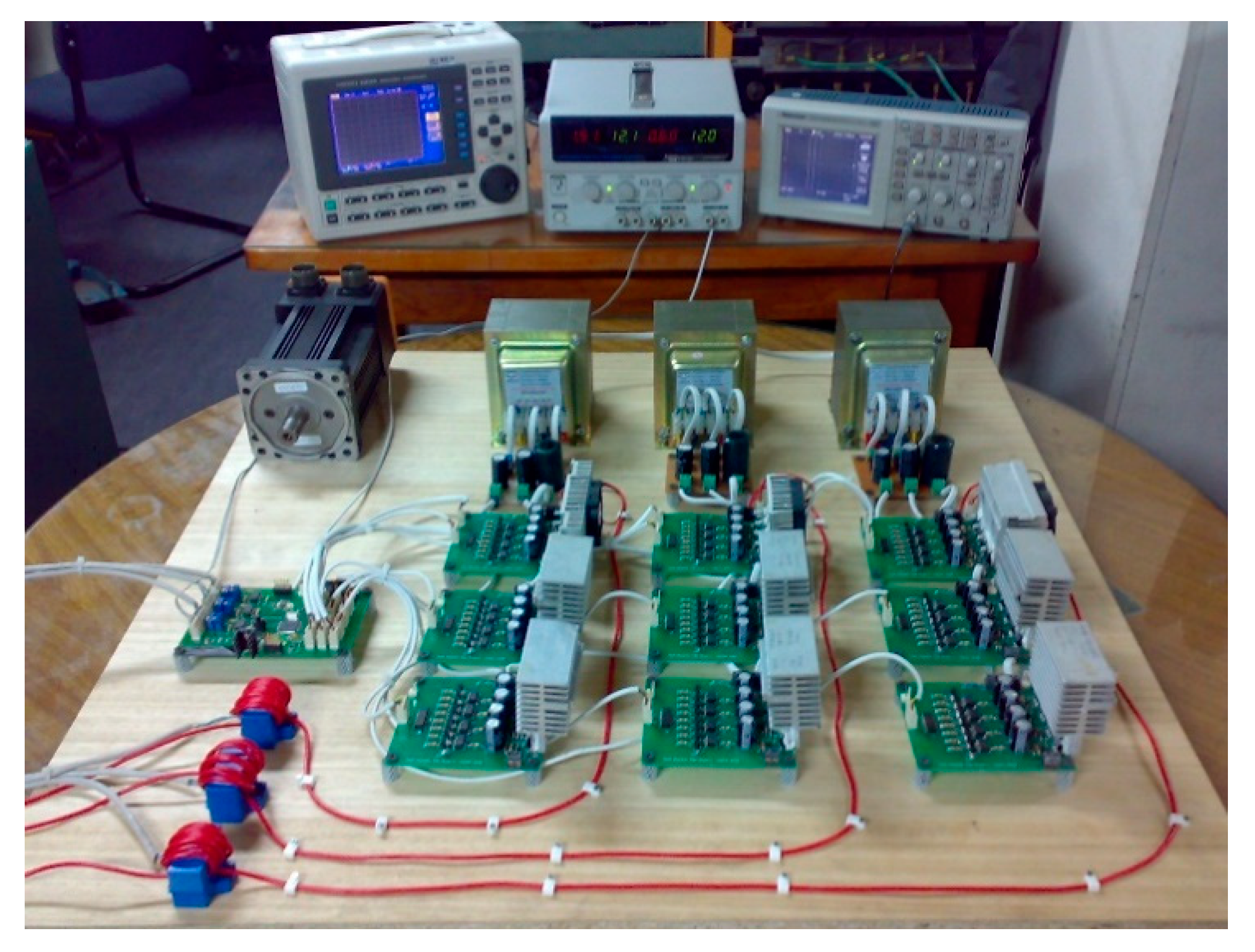
The list of components used for each Printed Circuit Board (PCB) that are part of the three-phase multi-level inverter with 27 levels of voltage per phase, as shown in Figure A1, designed and implemented in the Department of Electrical Engineering of Universidad de Santiago de Chile, is presented below:
- (1)
- List of components used in the implementation of each H-bridge board:
- IRF741 MOSFET.
- 74HC04N Hex inverter.
- 2N7000 MOSFET.
- MCT6 Optocoupler.
- 15 V Zener diode.
- 1N4007 Diode.
- (2)
- List of components used in the implementation of the control board:
- ATMEGA 1281 Microcomputer.
- LM1086 (5 V) Linear voltage regulator.
- LM317 (12 V) Adjustable linear voltage regulator.
- 2N7002 MOSFET.
- LM741OPAM.
- MAX3238 Voltage adapter for serial port.
- ADR550 Voltage reference.
Figure A1.
Three-phase multi-level inverter with 27 levels of voltage per phase.

References
- Urrea, C.; Kern, J. Fault-Tolerant Controllers in Robotic Manipulators. Performance Evaluations. IEEE Lat. Am. Trans. 2013, 11, 1318–1324. [Google Scholar] [CrossRef]
- Urrea, C.; Coltters, J.P. Design and Implementation of a Graphic 3D Simulator for the Study of Control Techniques Applied to Cooperative Robots. Int. J. Control Automat. Syst. 2015, 13, 1476–1485. [Google Scholar] [CrossRef]
- Urrea, C.; Pascal, J. Design, Simulation, Comparison and Evaluation of Parameter Identification Methods for an Industrial Robot. Comput. Electr. Eng. 2018, 67, 791–806. [Google Scholar] [CrossRef]
- Chen, J.; Duan, W.; Yang, X.; Zhang, L.; Shan, Y.; Yang, B.; Shu, H.; An, N.; Yu, T. Overall Adaptive Controller Design of PMSG Under Whole Wind Speed Range: A Perturbation Compensation Based Approach. Processes 2019, 7, 732. [Google Scholar] [CrossRef] [Green Version]
- García-Martínez, J.; Cruz-Miguel, E.; Carrillo-Serrano, R.; Mendoza-Mondragón, F.; Toledano-Ayala, M.; Rodríguez-Reséndiz, J. A PID-Type Fuzzy Logic Controller-Based Approach for Motion Control Applications. Sensors 2020, 20, 5323. [Google Scholar] [CrossRef] [PubMed]
- Borys, S.; Kaczmarek, W.; Laskowski, D. Selection and Optimization of the Parameters of the Robotized Packaging Process of One Type of Product. Sensors 2020, 20, 5378. [Google Scholar] [CrossRef]
- Urrea, C.; Matteoda, R. Development of a virtual Reality Simulator for a Strategy for Coordinating Cooperative Manipulator Robots Using Cloud Computing. Rob. Auton. Syst. 2020, 126, 103447. [Google Scholar] [CrossRef]
- Wu, K.; Kuhlenkoetter, B. Experimental Analysis of the Dynamic Stiffness in Industrial Robots. Appl. Sci. 2020, 10, 8332. [Google Scholar] [CrossRef]
- Urrea, C.; Kern, J. Characterization, Simulation and Implementation of a New Dynamic Model for a DC Servomotor. IEEE Lat. Am. Trans. 2014, 12, 997–1004. [Google Scholar] [CrossRef]
- Kang, H.; Zhou, H.; Wang, X.; Chen, C. Real-Time Fruit Recognition and Grasping Estimation for Robotic Apple Harvesting. Sensors 2020, 20, 5670. [Google Scholar] [CrossRef]
- Nguyen, H.T.; Trinh, V.C.; Le, T.D. An Adaptive Fast Terminal Sliding Mode Controller of Exercise-Assisted Robotic Arm for Elbow Joint Rehabilitation Featuring Pneumatic Artificial Muscle Actuator. Actuators 2020, 10, 118. [Google Scholar] [CrossRef]
- Kaczmarek, W.; Panasiuk, J.; Borys, S.; Banach, S. Industrial Robot Control by Means of Gestures and Voice Commands in Off-Line and On-Line Mode. Sensors 2020, 20, 6358. [Google Scholar] [CrossRef]
- Urrea, C.; Saa, D. Design and Implementation of a Graphic Simulator for Calculating the Inverse Kinematics of a Redundant Planar Manipulator Robot. Appl. Sci. 2020, 10, 6770. [Google Scholar] [CrossRef]
- Prianto, E.; Kim, M.S.; Park, J.H.; Bae, J.H.; Kim, J.S. Path Planning for Multi-Arm Manipulators Using Deep Reinforcement Learning: Soft Actor–Critic with Hindsight Experience Replay. Sensors 2020, 20, 5911. [Google Scholar] [CrossRef]
- Vysocký, A.; Papřok, R.; Šafařík, J.; Kot, T.; Bobovský, Z.; Novák, P.; Snášel, V. Reduction in Robotic Arm Energy Consumption by Particle Swarm Optimization. Appl. Sci. 2020, 10, 8241. [Google Scholar] [CrossRef]
- Oyekan, J.; Farnsworth, M.; Hutabarat, W.; Miller, D.; Tiwari, A. Applying a 6 DoF Robotic Arm and Digital Twin to Automate Fan-Blade Reconditioning for Aerospace Maintenance, Repair, and Overhaul. Sensors 2020, 20, 4637. [Google Scholar] [CrossRef] [PubMed]
- Urrea, C.; Kern, J.; Alvarado, J. Design and Evaluation of a New Fuzzy Control Algorithm Applied to a Manipulator Robot. Appl. Sci. 2020, 10, 7482. [Google Scholar] [CrossRef]
- Yang, Q.; Li, X.; Wanga, Y.; Ainapurea, A.; Lee, J. Fault Diagnosis of Ball Screw in Industrial Robots Using Non-Stationary Motor Current Signals. Proc. Manufact. 2020, 48, 1102–1108. [Google Scholar] [CrossRef]
- Schauder, C. Adaptive Speed Identification for Vector Control of Induction Motors without Rotational Transducers. IEEE Trans. Ind. Appl. 1992, 28, 1054–1061. [Google Scholar] [CrossRef]
- Levi, E.; Vukosavic, S.N.; Jones, M. Vector Control Schemes for Series Connected Six-Phase Two-Motor Drive Systems. IEE Proc. Elect. Power Appl. 2005, 15, 226–238. [Google Scholar] [CrossRef] [Green Version]
- Muktar, T.; Umale, A.; Kirpane, R. Vector Control Methods for Variable Speed of AC Motors. Int. Res. J. Eng. Tech. (IRJET) 2017, 4, 340–343. [Google Scholar]
- Nabae, A.; Takahashi, I.; Akagi, H. A New Neutral-Point-Clamped PWM Inverter. IEEE Ind. Appl. 1980, 2, 761–766. [Google Scholar] [CrossRef]
- Meynard, T.; Foch, H. Multilevel Converters and Derived Topologies for High Power Conversion. In Proceedings of the IECON ’95—21st Annual Conference on IEEE Industrial Electronics, Orlando, FL, USA, 6–10 November 1995; pp. 21–26. [Google Scholar] [CrossRef]
- Tolbert, L.; Peng, F. Multilevel Converters for Large Electric Drives. IEEE Trans. Ind. Appl. 1999, 35, 36–44. [Google Scholar] [CrossRef] [Green Version]
- Cherchali, N.O.; Tlemçani, A.; Boucherit, M.S.; Barazane, L. Comparative Study between Different Modulation Strategies for Five Levels NPC Topology Inverter. Energ. Pow. Eng. 2011, 3, 276–284. [Google Scholar] [CrossRef] [Green Version]
- Manias, S.N. A New Neutral-Point-Clamped PWM Inverter. Pow. Electr. Motor Drive Sys. 2017, 2, 761–766. [Google Scholar]
- Suresh, Y.; Venkataramanaiah, J.; Panda, A.K.; Dhanamjayulu, C.; Venugopal, P. Investigation on cascade multilevel inverter with symmetric, asymmetric, hybrid and multi-cell configurations. Ain Shams Eng. J. 2017, 8, 263–276. [Google Scholar] [CrossRef]
- Manias, S.N. Introduction to Motor Drive Systems. In Power Electronics and Motor Drive Systems; School of Electrical and Computer Engineering, National Technical University of Athens: Athens, Greece, 2017; pp. 843–967. [Google Scholar]
- Wang, Y.; Yu, H.; Che, Z.; Wang, Y.; Zeng, C. Extended State Observer-Based Predictive Speed Control for Permanent Magnet Linear Synchronous Motor. Processes 2019, 7, 618. [Google Scholar] [CrossRef] [Green Version]
- Zheng, J.; Yuan, Y.; Zou, L.; Deng, W.; Guo, C.; Zhao, H. Study on a Novel Fault Diagnosis Method Based on VMD and BLM. Symmetry 2019, 11, 747. [Google Scholar] [CrossRef] [Green Version]
- Yao, X.; Zhao, J.; Lu, G.; Lin, H.; Wang, J. Commutation Error Compensation Strategy for Sensorless Brushless DC Motors. Energies 2019, 12, 203. [Google Scholar] [CrossRef] [Green Version]
- Lee, C.Y.; Wen, M.S. Establish Induction Motor Fault Diagnosis System Based on Feature Selection Approaches with MRA. Processes 2020, 8, 1055. [Google Scholar] [CrossRef]
- Worku, M.; Hassan, M.; Abido, M. Real Time Energy Management and Control of Renewable Energy based Microgrid in Grid Connected and Island Modes. Energies 2019, 12, 276. [Google Scholar] [CrossRef] [Green Version]
- Rodríguez, J.; Lai, J.S.; Peng, F.Z. Multilevel inverters: A survey of topologies, controls, and applications. IEEE Trans. Ind. Elect. 2002, 49, 724–738. [Google Scholar] [CrossRef] [Green Version]
- Colak, I.; Kabalci, E.; Bayindir, R. Review of multilevel voltage source inverter topologies and control schemes. Energy Conv. Manag. 2011, 52, 1114–1128. [Google Scholar] [CrossRef]
- Jacob, J.; Chitra, A. Field Oriented Control of Space Vector Modulated Multilevel Inverter fed PMSM Drive. Energy Procedia 2017, 117, 966–973. [Google Scholar] [CrossRef]
- Chitra, A.; Sultana, R.; Vanishree, J.; Sreejith, S.; Jose, S.; Pulickan, A.J. Performance Comparison of Multilevel Inverter Topologies for Closed Loop v/f Controlled Induction Motor Drive. Energy Procedia 2017, 117, 958–965. [Google Scholar] [CrossRef]
- Sinha, A.; Jana, K.C.; Das, M.K. An inclusive review on different multi-level inverter topologies, their modulation and control strategies for a grid connected photo-voltaic system. Solar Energy 2018, 170, 633–657. [Google Scholar] [CrossRef]
- Blaabjerg, F. Basic Control of AC Motor Drives. In Control of Power Electronic Converters and Systems, 1st ed.; Lee, K.B., Shin, H.U., Bak, Y., Eds.; Academic Press: Cambridge, MA, USA, 2018; pp. 301–329. [Google Scholar]
- Rashid, M.H. Motor Drives. In Power Electricity Handbook, 4th ed.; Rahman, M.F., Patterson, D., Cheok, A., Betz, R., Eds.; Florida Polytechnic University: Lakeland, FL, USA, 2018; pp. 945–1021. [Google Scholar]
- Verelli, C.M.; Tomei, P. AC motors: Letter swap potentialities. Automatica 2020, 1130, 108763. [Google Scholar] [CrossRef]
Figure 1.
Electric scheme of three-phase multi-level inverter with 27 levels of voltage per phase connected to an ACBPMM.
Figure 1.
Electric scheme of three-phase multi-level inverter with 27 levels of voltage per phase connected to an ACBPMM.

Figure 2.
Dynamic model of 2- DoF robot.

Figure 3.
General scheme of position control system.

Figure 4.
Scheme of variable PID control strategy.

Figure 5.
Interpolation scheme for the calculation of the P proportional gain of a PID controller using gain scheduling by interpolation of a linear polynomial.
Figure 5.
Interpolation scheme for the calculation of the P proportional gain of a PID controller using gain scheduling by interpolation of a linear polynomial.

Figure 6.
Movement of first link from 0° to 15°.

Figure 7.
Movement of first link from 15° to 35°.

Figure 8.
Movement of first link from 60° to 75°.

Figure 9.
Stability analysis of the first link at 45°.

Figure 10.
Analysis of IA, RMS, and RSD errors of the control strategies applied in the first link of the robotic arm.
Figure 10.
Analysis of IA, RMS, and RSD errors of the control strategies applied in the first link of the robotic arm.

Figure 11.
Robotic arm movement: first link from 0° to 15° and second link from 0 (m) to 0.04 (m).

Figure 12.
Robotic arm movement: first link from 15° to 35° and second link from 0 (m) to 0.03 (m).

Figure 13.
Robotic arm movement: first link from 60° to 75° and second link from 0 (m) to 0.04 (m).

Figure 14.
Stability analysis of the robotic arm: first link at 45° and second link at 0.02 (m).

Figure 15.
Analysis of the IA, RMS, and RSD errors of the control strategies applied in the two links of the robotic arms.
Figure 15.
Analysis of the IA, RMS, and RSD errors of the control strategies applied in the two links of the robotic arms.

Figure 16.
Reference pattern for robotic arm.

Figure 17.
Movement of each link of the robotic arm when following the reference pattern in the Cartesian plane.
Figure 17.
Movement of each link of the robotic arm when following the reference pattern in the Cartesian plane.

Figure 18.
Movement of each link of the robotic arm when this follows the reference pattern, and mechanical disturbances.
Figure 18.
Movement of each link of the robotic arm when this follows the reference pattern, and mechanical disturbances.

Figure 19.
Analysis of IA, RMS, and RSD errors of the control strategies when the robotic arm follows the reference pattern.
Figure 19.
Analysis of IA, RMS, and RSD errors of the control strategies when the robotic arm follows the reference pattern.


Table 1.
Parameters of a three-phase synchronous brushless motor.
| Description | Value |
|---|---|
| Power | 750 (W) |
| Number of pole pairs | 4 |
| Synchronous inductance | 6.4 (mH) |
| Synchronous resistance | 2.88 (Ω) |
| Moment of inertia | 2.42 · 10−4 (Kg · m 2) |
| Viscous friction | 0.002 (N · m · s) |
| Flux density generated by the rotor magnet | 0.17351 (Wb) |
Table 2.
Scheme of PID parameters per angular position range of the robotic arm.
| Range | Kp | Ki | Kd |
|---|---|---|---|
| 0°–θ1 | Kp1 = 0.093 | Ki1 = 0.008 | Kd1 = 0.5 |
| θ1–θ2 | Kp2 = 0.178 | Ki2 = 0.010 | Kd2 = 1.0 |
| θ2–θ3 | Kp3 = 0.212 | Ki3 = 0.012 | Kd3 = 1.1 |
| θ3–θ4 | Kp4 = 0.249 | Ki4 = 0.139 | Kd4 = 1.3 |
| θ4–90° | Kp5 = 0.296 | Ki5 = 0.224 | Kd5 = 2.1 |
Publisher’s Note: MDPI stays neutral with regard to jurisdictional claims in published maps and institutional affiliations. |
© 2021 by the authors. Licensee MDPI, Basel, Switzerland. This article is an open access article distributed under the terms and conditions of the Creative Commons Attribution (CC BY) license (http://creativecommons.org/licenses/by/4.0/).
Share and Cite
MDPI and ACS Style
Urrea, C.; Jara, D. Design, Analysis, and Comparison of Control Strategies for an Industrial Robotic Arm Driven by a Multi-Level Inverter. Symmetry 2021, 13, 86. https://doi.org/10.3390/sym13010086
AMA Style
Urrea C, Jara D. Design, Analysis, and Comparison of Control Strategies for an Industrial Robotic Arm Driven by a Multi-Level Inverter. Symmetry. 2021; 13(1):86. https://doi.org/10.3390/sym13010086
Chicago/Turabian StyleUrrea, Claudio, and Daniel Jara. 2021. "Design, Analysis, and Comparison of Control Strategies for an Industrial Robotic Arm Driven by a Multi-Level Inverter" Symmetry 13, no. 1: 86. https://doi.org/10.3390/sym13010086
Note that from the first issue of 2016, this journal uses article numbers instead of page numbers. See further details here.