
A Bimodal Extension of the Exponential Distribution with Applications in Risk Theory


1
Department of Mathematics, Faculty of Basic Science, University of Antofagasta, Antofagasta 02800, Chile
2
Department of Quantitative Methods and Institute of Tourism and Sustainable Economic Development (TIDES), University of Las Palmas de Gran Canaria, 35017 Las Palmas, Spain
3
Centre for Actuarial Studies, Department of Economics, University of Melbourne, Parkville, VIC 3010, Australia
*
Author to whom correspondence should be addressed.
Symmetry 2021, 13(4), 679; https://doi.org/10.3390/sym13040679
Submission received: 12 March 2021
/
Revised: 4 April 2021
/
Accepted: 6 April 2021
/
Published: 14 April 2021
(This article belongs to the Special Issue Symmetric and Asymmetric Bimodal Distributions with Applications)
Abstract
:There are some generalizations of the classical exponential distribution in the statistical literature that have proven to be helpful in numerous scenarios. Some of these distributions are the families of distributions that were proposed by Marshall and Olkin and Gupta. The disadvantage of these models is the impossibility of fitting data of a bimodal nature of incorporating covariates in the model in a simple way. Some empirical datasets with positive support, such as losses in insurance portfolios, show an excess of zero values and bimodality. For these cases, classical distributions, such as exponential, gamma, Weibull, or inverse Gaussian, to name a few, are unable to explain data of this nature. This paper attempts to fill this gap in the literature by introducing a family of distributions that can be unimodal or bimodal and nests the exponential distribution. Some of its more relevant properties, including moments, kurtosis, Fisher’s asymmetric coefficient, and several estimation methods, are illustrated. Different results that are related to finance and insurance, such as hazard rate function, limited expected value, and the integrated tail distribution, among other measures, are derived. Because of the simplicity of the mean of this distribution, a regression model is also derived. Finally, examples that are based on actuarial data are used to compare this new family with the exponential distribution.
MSC:
62-07; 62P05; 62E991. Introduction
It is well-known that many empirical datasets that are traditionally used in different scenarios, such as financial econometrics, actuarial, income modelling, and industrial engineering, include positive support and bimodality. For example, in the stochastic frontier model, it can be assumed that some firms are fully efficient. In contrast, others are inefficient, giving to an error term that can be bimodal (see, for example, the recent work of [1]). In this case, the problem is to assess which regime (efficient or inefficient) each firm belongs to. The result of the distribution of the disturbance term can be, in this case, bimodal. Furthermore, in some cases, the classical continuous distributions can neither account for zero values in its support nor reach two maxima. In this regard, many empirical continuous data with positive support begins at zero, including a high frequency of this initial value. This portion of observations is neither negligible, nor should they be ignored. Because most of the aforementioned classical distributions are not allowed to incorporate the zeroes, most of the researchers truncate the data by omitting those values or modelling with mixed random variables that include a mixture of a classical distribution and a point mass 0 (see [2]). Although numerous models have been developed in discrete scenarios, e.g., zero-inflated and hurdles models, which can perfectly describe the excess of zeros, this is not the case in the continuous case.
Being motivated by this idea, this work introduces a family of distributions with support in that satisfactorily adapts to the unimodal or bimodal nature of the empirical data. Our objective, following the methodology shown in [3], consists of incorporating an additional parameter , in a parent distribution, e.g., exponential, gamma, to build a more flexible probability model. This parameter controls the unimodality or bimodality of the proposed family. The particular case is reduced to the starting distribution. In that work, the author incorporates a methodology that is conducive to generating asymmetry and sometimes bimodality starting from the normal distribution. The idea here is to use this methodology for the general case of starting from any distribution. In this paper, special attention is paid to the parent distribution case is the exponential one. After providing the expression of the probability density function (pdf) of the proposed distribution, we study some of its more relevant properties, such as moments, kurtosis, Fisher’s asymmetric coefficient, and some estimation methods. A regression model can also be derived by reparameterizing the mean of this new distribution. Several examples that are based on actuarial data are discussed and the performance of this model is compared with the exponential distribution. Note that other generalizations of the exponential distribution have been considered by [4,5] and also by [6]. Nevertheless, these generalizations of the exponential model are not able to incorporate covariates. Although the methodology that is developed in this work is fully parametric, there has been an increasing number of publications to discuss similar problems within the field of machine learning and statistical framework, see, for example [7,8,9], among others.
On the other hand, a weighted distribution is a powerful tool to enhance a parent discrete or continuous distribution. Recall that, for a random variable X with support in with probability density function that depends on a parameter (or vector of parameters) , it can be constructed a new distribution via a weighted function, , with probability density function (see for instance [10,11,12])
where is a new parameter and where it is assumed that . Now, by combining this methodology with the idea that is given in [3], a result that provides a generalization of a classical continuous distribution is proposed. The resulting model can be either unimodal or bimodal, as shown in the following Proposition.
Proposition 1.
Let a continuous distribution with finite mean μ and variance . Subsequently, it is verified that
with . The latter parameter controls the unimodality or the bimodality of the distribution and
is a genuine pdf.
Proof.
The result is obtained by considering that and integrating over the support of the random variable Y to have . □
The parameter controls the unimodality or bimodality of the distribution. Additionally, by taking , the parent pdf is obtained as a special case. Subsequently, the methodology proposed in Proposition 1 is a method to generalize a parent pdf.
The probability density function that is given in (2) can be viewed as a weighted distribution. There exists a vast literature dealing with the construction of such distributions in the discrete case since the pioneering work of [10]. However, the literature regarding the continuous scenario is scarce. The idea behind this construction is simple and it aims to obtain more flexible distributions that adapt to empirical data distributions. If the weight is the mean of the initial distribution, then the weighted function’s interpretation in terms of the length biased (size biased) sampling is possible. However, much more effort is required to obtain an interpretation of the function beyond incorporating a parameter that controls the unimodality or bimodality of the distribution obtained.
The cumulative distribution function (cdf) of this family is obtained by integrating (2) by parts
It is noted that the integral in the second term of the right-hand side of (3) is obtained in a closed-form under the classical distributions, such as the exponential, gamma, and Weibull. In this paper, we discuss the particular case in which the parent distribution is the exponential distribution. A comprehensive examination of its mathematical properties is carried out with relevant emphasis on results that are related to insurance. Additionally, parameter estimation is completed by the methods of moments and maximum likelihood. Moreover, we analyze the efficiency of the estimates via a simulation study. Finally, the model’s practical performance is examined by using two real claims size sets of data. The distribution that is proposed in this paper can be used as a basis for excess-of- loss quotations. Furthermore, it provides a good description of the random behaviour of significant losses, similarly to the Pareto distribution. Unlike other generalizations of the exponential distribution, the one introduced in this work allows for us to derive a regression model due to its mean simple expression.
The rest of the paper is organised, as follows. Section 2 provides some statistical properties of this model. Section 3 shows a catalogue of actuarial results. Next, Section 4 describes parameter estimation and a simulation study. The regression model is derived in Section 5. Numerical applications are given in Section 6 and the last Section concludes the paper.
2. Bimodal Extension of the Exponential Distribution
Let us first consider the classical exponential distribution with the pdf given by
with a rate parameter and a unique modal value located at . The survival function is . Henceforward, a random variable X that follows (4) will be denoted by .
Now, by using (2) and taking into account that and , we have that, for
where , the expression
is a genuine pdf for , and . The survival function is obtained from (3) and it is given by
with
The exponential distribution is obtained when . From now on, a random variable that Y follows the pdf (5) will be denoted as . Figure 1, below, shows the graphs of the pdf of this distribution for several values of the parameters and .
It can be easily verified that, if , then the shape of the distribution resembles the exponential one with a mode at . On the other hand, for other values of , the pdf reaches a local maximum (local mode) at
and a minimum (antimode) at
Furthermore, since , then the value of the pdf at zero is larger than the one of the classical exponential distribution at the same value for and lower in the rest of its domain.
Reliability, Hazard Rate Function and Moments
The reliability function and the hazard (failure) rate function are two important reliability measures. The reliability function of a random variable Y is defined as and it is given by (6), while the hazard rate function, defined as , is provided by
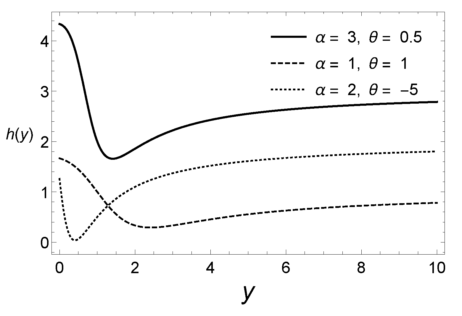
Figure 2 displays the hazard rate function of the law for different values of the parameters. As compared to the exponential distribution, which has a constant hazard rate, it is discernible that the hazard function of the distribution that is proposed here exhibits a wide variety of shapes. Therefore, the new family of distributions is flexible enough to describe a diversity of real datasets.
It is simple to see that the hazard rate function reaches a minimum at for and at for . Obviously, for the hazard rate function is constant, corresponding to the exponential case. The moment generating function is given by
from which we can derive the moments of the distribution; these are given by
where , and and are the mean and standard deviation of the exponential distribution respectively. Therefore, (8) can be rewritten as
In particular, the mean, second order moment, and variance are given by
It is straightforward to see that the mean decreases with for and increases in the rest of the support of this parameter.
The asymmetry coefficient (not given here) can be obtained in closed-form expression by using the well-known formula
where .
3. Results in Risk Theory
In this section, some interesting actuarial results of this family of distributions are provided. Let the random variable Y represent either a policy limit or reinsurance deductible (from an insurer’s perspective); then, the limited expected value function L of Y with cdf , is defined by
which is the expectation of the cdf . In other words, it represents the expected amount per claim that is retained by the insured on a policy with a fixed amount deductible of y. This is an appropriate tool for analyzing an excess of loss reinsurance ([13], Chapter 2, p. 59 and [14], Chapter 3, p. 113), among others. For the distribution, this amount is given by
where . The pdf (5) can be also applied to rating excess-of-loss reinsurance, as it can be seen in the following result.
Proposition 2.
Let Y be a random variable denoting the individual claims size taking values only for individual claims greater than d. Let us also assume that Y follows the pdf (5), then the expected cost per claim to the reinsurance layer when the loss in excess of m subject to a maximum of l is given by
where
Proof.
The result follows by taking into account that
from which we obtain the result after some algebra. □
The failure rate of the integrated tail distribution, as defined by
is given by
Additionally, the reciprocal of is the mean residual life that can be easily derived. In the insurance context (see, for example [13,15]) for a claims amount random variable Y, the mean excess function or mean residual life function, , plays an essential role in reinsurance framework. It is interpreted as the expected payment per claim on a policy with a fixed deductible of y, where claims with an amount less than or equal to y is completely ignored. Because the mean residual life is related to the limited expected value function through the expression (see [13], p. 59)
a closed-form expression can be obtained for the mean residual life
Finally, the TVaR function is also provided in closed-form,
4. Methods of Estimation and Simulation
Given a random sample taken from the distribution, simple moment estimates can be calculated by equating the sample and theoretical moments. Because there are two parameters, we need, for example, the mean, , and the sample second order moment around the origin, . Now, by setting equal (9) and (10) to the sample counterparts, we get
By plugging (13) into (10), we obtain the equation
which depends solely on and it can be solved numerically. The impossibility of proving that both moment and maximum likelihood estimators exist and are unique is one of the most substantial limitations of the proposed probabilistic model. However, in practice, the model’s estimates, as shown in the simulation analysis and numerical applications, are easily obtained by numerical methods without difficulty. This issue leads us to think that they correspond to global maxima, although they cannot be guaranteed.
We now proceed with the maximum likelihood method of estimation. The log-likelihood function can be written as
where . Then, the normal equations are given by
with, , and
Numerical procedures, such as the Newton–Raphson algorithm can be used to derive the solutions of the system of equations that are given by (14) and (15). Unlike the exponential distribution, the maximum likelihood estimates cannot be expressed in closed-form. In practice, as we are unable to prove that the log-likelihood function is concave, the likelihood function can be directly maximized by considering different values as seed points, since the global maximum is not guaranteed by the impossibility to prove that the log-likelihood function is concave. We have used different maximum search methods available in the FindMaximum built-in function in Mathematica software package. These methods include the Newton–Raphson and the Broyden–Fletcher–Goldfarb-Shanno (BGGS) algorithms. The same results were achieved under these two optimization functions. Although a more general structure, such as kernel regression or neural network, could provide accurate estimates, the approach used in this paper does not require training data. It can also work well, even if the fit to data is not perfect. Additionally, this method is easier to understand and interpret results, i.e., a parametric test for the significance of the parameter estimates can lead to a rejection of the null hypothesis rather than the non-parametric counterpart. Finally, from the actuarial perspective, the practitioner may be interested in the parametric approach since it provides appealing closed-form expressions, as is the case of this BE representation.
Simulation Experiment
Here, an acceptance-rejection algorithm to generate random variates from the distribution (see [16]) is used. The simulation analysis results are illustrated in Table 1, where the behaviour of the maximum likelihood estimates of 1000 simulated samples of sizes 50, 100, 150, and 200 from the distribution. For each simulated sample generated, the estimates were numerically computed via a Newton–Raphson algorithm. In this Table, the means, standard deviations (SD), and percentage of coverage probability (C) are reported for different values of the parameters and . As expected, it is observable that the bias becomes smaller as the sample size n increases.
5. A suitable Regression Model
In practice, to better explain the response variable, it is important that the statistical model is able to incorporate covariates. By rewriting (9) as
a reparameterization of the distribution in (5) is obtained, where . The variance of the reparameterized distribution is given by
where
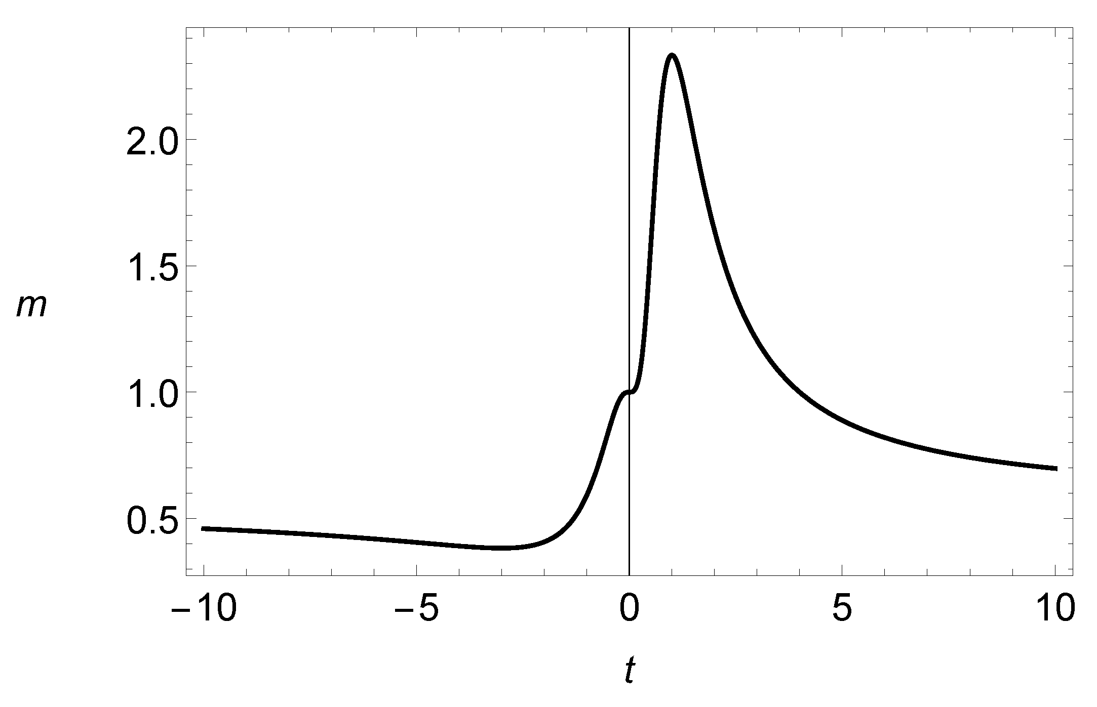
In this case, the parameter can be interpreted as a precision parameter, since the function increases for (see Figure 3) and decreases in the rest of the domain of . Thus, is the mean of the response variable and can be regarded as a precision parameter in the sense that, for a fixed value of , the variance of Y varies according to the values of , i.e., the values of the parameter .
Because the mean of the response is non-negative, the most common function that relates the mean and the linear predictor is the log link,
where is a q-vector of explanatory variables and is a q-vector of unknown regression coefficients that may include an intercept. Subsequently, we have the conventional log-linear model, such that with .
The maximum likelihood estimates of the regressors , can be computed via the Newton–Raphson algorithm. In our applications, parameters will be estimated by the maximum likelihood method by using this algorithm available in the software packages Mathematica [17] and RATS [18]. The code for the latter package is available upon request.
As is well-known, the marginal effect reflects the variation of the conditional mean of Y due to a one-unit change in the sth covariate, and it is calculated as for and . Thus, the marginal effect indicates that a one-unit change in the sth regressor increases or decreases the expectation of the dependent variable, depending on the sign, positive or negative, of the regressor for each mean. For indicator or dummy variables that take only the value 0 or 1, the marginal effect in term of the odds-ratio is approximately . Therefore, the conditional mean is times larger if the indicator variable is one rather than zero.
6. Empirical Results
Two datasets will be used to illustrate the applicability of the distribution studied in this paper. The first one is related to life insurance and the other one to non-life insurance. For these two examples considered, the exponential distribution and the zero-adjusted gamma model provided in [2] will be used as a benchmark. The pdf of this last distribution is given by
where , , . This mixture distribution will be denoted hereafter as . It is worthy to point out that other versions of the generalized exponential distribution, such as the one that was proposed by [4], and the one suggested by [5], do not yield significant improvement over the model introduced in this work.
6.1. Dataset 1
Life insurers offer new products to increase their market share, as is the case in the majority of financial companies that operate in the markets. Thus, insurance companies need to know specific characteristics of their potential customers, which makes it is crucial to update their databases accordingly to include the appropriate information. In this first example, we use data from the Consumer Finance Survey (SCF), a representative sample at the national level (in the U.S.) of 500 households with positive income who were interviewed in the survey that was conducted in 2004. For term life insurance, the amount of insurance is measured by the policy face, the amount that the company will pay in the event of the death of the named insured. Important characteristics that may impact this quantity (covariates) are shown in some detail in Table 2. This dataset can be found in the personal website of Professor E. Frees (Wisconsin School of Business Research), https://instruction.bus.wisc.edu/jfrees/jfreesbooks/Regression%20Modeling/BookWebDec2010/data.html.
Parameter estimates obtained by the method of maximum likelihood together with standard errors (in brackets) are illustrated in Table 3 and Table 4 for the model without and with covariates, respectively. As it can be observed, the model proposed in this paper provides a better fit to this dataset than the exponential distribution in both cases in terms of three measures of model selection, maximum of the log-likelihood function, AIC and CAIC. The expressions of the latter measures are:
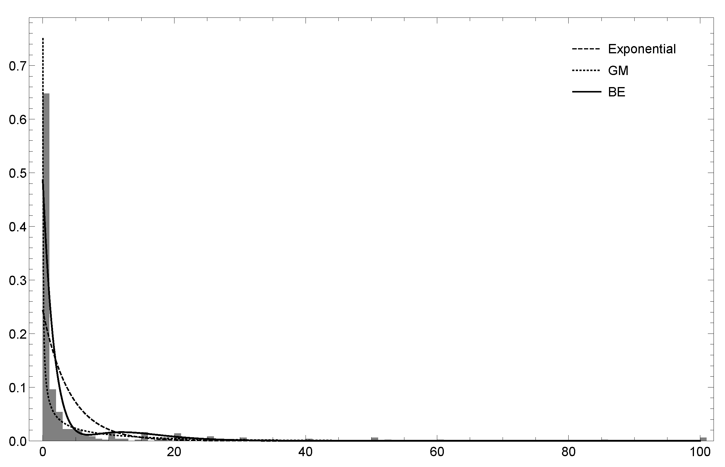
where k is the number of parameters, and n is the sample size. A model with a lower value of these measures is preferable. It is also discernible in Figure 4 that the distribution is able to reproduce the bimodality of the empirical data. Also, in Table 4 are displayed the estimates, standard errors (S.E.), t-Wald statistics and p-values for the and exponential (in brackets) distributions. It can be noticed that the sign of some of the estimated regressors differs in the sign for both models. Besides, most of the explanatory variables (except for and ) are statistically significant at the 5% significance level. Similarly to the previous case, according to the same model validation measures, the provides a better fit to data.
6.2. Dataset 2
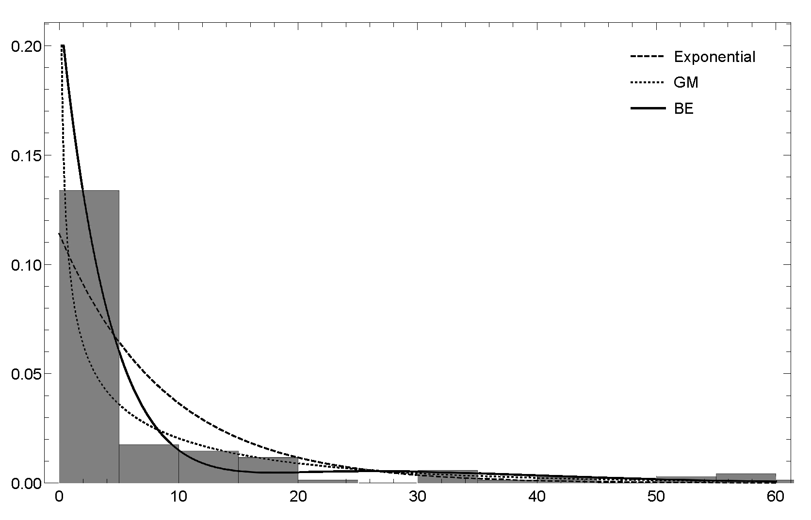
This second example discusses a cross-sectional dataset that was collected in 1977 related to third party car insurance claims. It can also be found in the website of Professor E. Frees. See also [19] and the references therein. The explanatory variables of interest are described below in Table 5. Using these explanatory variables, we explain the response variable, the payments in Swedish krona (variable payment divided by ). Only 136 data observations out of the total 2182 observations correspond to the case where the insured is classified in the bonus scale 1 (insured starts in class 1 and it is moved up one class, to a maximum of 7 after a claim-free year). Therefore, in this application, only those insureds with a lesser driving experience have been considered since the empirical distribution shows bimodality.
The estimates of the basic model (without covariates) and standard errors are exhibited in Table 3. Once again, the distribution provides a better fit to data than the exponential model in terms of the three measures of model selection.
Moreover, Table 6 shows the estimates, standard errors (S.E.), t-Wald statistics, and p-values for the and exponential (in brackets) distributions. It is noted that there are no significant differences with respect to the exponential regression model, except for the variable make, which is not statistically at the usual significance levels under the new regression model.
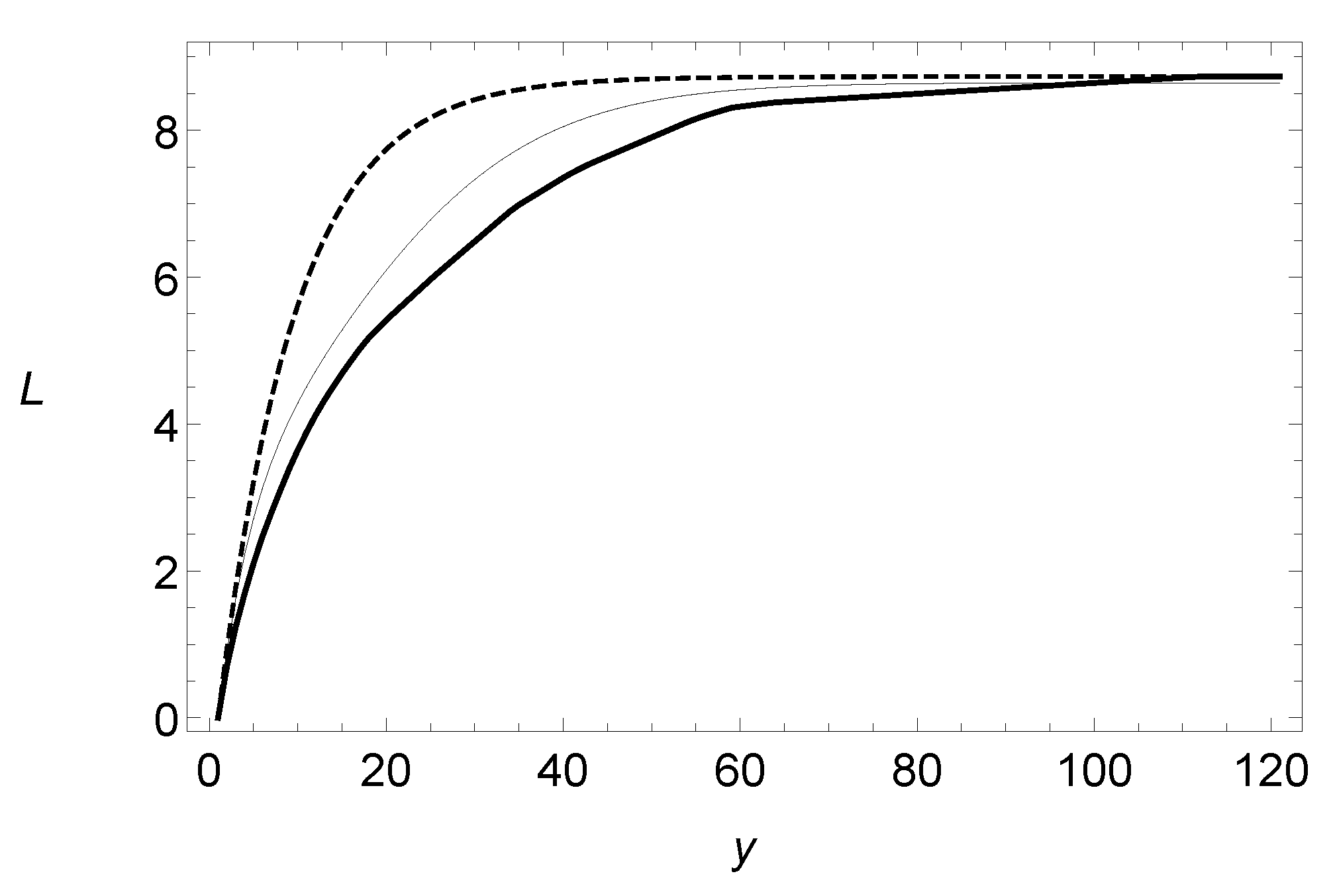
Similarly to the previous example (see Figure 5), the new model can also reproduce the second mode of the empirical data. Finally, we have computed the limited expected values tha are given in (12) for the basic model, without including covariates, and compared those numerical figures with the empirical values and those obtained for the exponential distribution. It is apparent that, for the distribution, the computed values adhere closer to the empirical ones than those ones that are derived from the exponential model (see Figure 6).
Now, we are interested in analyzing the out-of-sample performance of the distribution. For that reason, we have randomly partitioned the second dataset into two disjoint subsets of the same size. The first subset of size 68 is used for fitting the models, whereas the second subset tests the model’s out-of-sample prediction accuracy. We have fitted the exponential and the distribution to these datasets. Subsequently, we compare the out-of-sample performance via the likelihood ratio test proposed by [20] for non-nested models. The test statistic of Vuong’s closeness test is
is the sample variance of the pointwise log-likelihood ratios and and represent the pdf of two different non-nested models, and are the maximum likelihood estimates of and and and are the number of estimated parameters in the model with pmf and , respectively. Note that the Vuong’s statistic is sensitive to the number of estimated parameters in each model and, therefore, the test must be corrected for dimensionality. We test against . Under the null hypothesis, T is asymptotically normally distributed. At the 5% significance level, the rejection region for this test in favour of the alternative hypothesis occurs when . By following this approach, we have calculated the test statistics of the Vuong’s test 1000 times. The resulting average value of the test statistics was , then the regression model is preferable to the exponential regression model at the 5% significance level, in-sample and out-of-sample, for this dataset.
Apart from improving the maximum value of the likelihood function, it is interesting to note that the estimation of the parameters is fast from a computational point of view and not problematic. Bear in mind that, to obtain bimodal modelling, a finite mixture of two distributions, such as the gamma exponential, may be possible. Still, in these cases, the estimation of the parameter that weighs both distributions can give rise to identifiability problems.
7. Conclusions and Extensions
In this paper, a methodology that allows us to generalize an initial probability distribution by adding a parameter that controls the unimodality or bimodality of the new family was introduced. Special attention was paid to the case where the parent model is the exponential distribution, thus obtaining a new generalization of the exponential distribution that can be considered to be an alternative model to other extensions of this distribution. This new model’s analytical expression is simple, and many interesting statistical and actuarial quantities are obtained in closed-form. The derivation of composite and folded models that are based on this bimodal family might be a line of further research following the recent works of [21,22], among others.
Finally, the computation of the disturbance term’s distribution in the stochastic frontier analysis assuming the bimodal exponential distribution as the distribution of the inefficiency and a normal distribution of the noise can be obtained in a closed-form expression. This distribution can be bimodal, thus it is a suitable model for explaining different sources of inefficiency. We believe that this is a promising line of research to be addressed in the future.
Author Contributions
Conceptualization, J.R. and H.W.G.; methodology, J.R and E.G.-D.; software, E.G.-D. and E.C.-O.; validation, E.G.-D. and E.C.-O.; formal analysis, J.R.; resources, H.W.G.; data curation, E.G.-D.; writing—original draft preparation, E.G.-D.; writing—review and editing, E.C.-O.; funding acquisition, H.W.G. All authors have read and agreed to the published version of the manuscript.
Funding
The research of J. Reyes and H.W. Gómez was supported by MINEDUC-UA project, code ANT 1755 (Chile) and SEMILLERO UA-2021 (Chile). EGD work was partially funded by grant ECO2017–85577–P (Ministerio de Economía, Industria y Competitividad. Agencia Estatal de Investigación).
Institutional Review Board Statement
Not applicable.
Informed Consent Statement
Not applicable.
Data Availability Statement
Data supporting reported results can be found in the personal website of E. Frees (Wisconsin School of Business Research), https://instruction.bus.wisc.edu/jfrees/jfreesbooks/Regression%20Modeling/BookWebDec2010/data.html.
Acknowledgments
The authors are grateful to the two anonymous referees for their constructive comments and suggestions, which have greatly helped us improve the manuscript. EGD also acknowledges the Departamento de Matemáticas, Facultad de Ciencias Básicas, Universidad de Antofagasta, Antofagasta (Chile) for their special support, as part of this paper was done while EGD was visiting this University in 2018.
Conflicts of Interest
The authors declare no conflict of interest.
References
- Kumbhakar, S.; Parmeter, C.; Tsionas, E.G. A zero inefficiency stochastic frontier model. J. Econ. 2013, 172, 66–76. [Google Scholar] [CrossRef]
- Tong, N.; Christophe, M.; Thomas, L. A zero-adjusted gamma model for mortgage loan loss given default. Int. J. Forecast. 2013, 29, 548–562. [Google Scholar] [CrossRef] [Green Version]
- Elal-Olivero, D. Alpha-skew-normal distribution. Proyecciones 2010, 29, 224–240. [Google Scholar] [CrossRef] [Green Version]
- Marshall, A.; Olkin, I. A new method for adding a parameter to a family of distributions with application to the exponential and Weibull families. Biometrika 1997, 84, 641–652. [Google Scholar] [CrossRef]
- Gupta, P.K.; Kundu, D. Generalized exponential distributions. Aust. N. Z. J. Stat. 1999, 41, 173–188. [Google Scholar] [CrossRef]
- Gómez-Déniz, E. Adding a parameter to the exponential and Weibull distributions with applications. Math. Comput. Simul. 2017, 144, 108–119. [Google Scholar] [CrossRef]
- Kuhn, D.; Mohajerin, P.; Nguyen, V.; Abadeh, S. Wasserstein Distributionally Robust Optimization: Theory and Applications in Machine Learning. In Operations Research & Management Science in the Age of Analytics; Informs: Catonsville, MD, USA, 2019; pp. 130–166. [Google Scholar]
- Imani, M.; Ghoreishi, S. Scalable Inverse Reinforcement Learning Through Multifidelity Bayesian Optimization. IEEE Trans. Neural Netw. Learn. Syst. 2021, 1–8. [Google Scholar] [CrossRef]
- Bellemare, M.G.; Dabney, W.; Munos, R. A Distributional Perspective on Reinforcement Learning. In Proceedings of the 34th International Conference on Machine Learning, Sydney, NSW, Australia, 6–11 August 2017; Precup, D., Teh, Y.W., Eds.; International Convention Centre: Sydney, NSW, Australia, 2017; Volume 70, pp. 449–458. [Google Scholar]
- Fisher, R. The effects of methods of ascertainmenut pon the estimation of frequencies. Ann. Eugen. 1934, 6, 13–25. [Google Scholar] [CrossRef]
- Harandi, S.S.; Alamtsaz, M. Discrete alpha-skew-Laplace distribution. SORT 2013, 39, 71–84. [Google Scholar]
- Patil, G.; Rao, C. Weighted distributions and size biased sampling with applications to wildlife populations and human families. Biometrics 1978, 34, 179–184. [Google Scholar] [CrossRef] [Green Version]
- Hogg, R.; Klugman, S. Loss Distributions; John Wiley and Sons: New York, NY, USA, 1984. [Google Scholar]
- Boland, P. Statistical and Probabilistic Methods in Actuarial Science; Chapman & Hall: London, UK, 2007. [Google Scholar]
- Klugman, S.; Panjer, H.; Willmot, G. Loss Models: From Data to Decisions, 3rd ed.; Wiley: Hoboken, NJ, USA, 2008. [Google Scholar]
- Von Newmann, J. Various Techniques used in Connection With Random Digits. Stand. Appl. Math. Ser. 1951, 12, 36–38. [Google Scholar]
- Ruskeepaa, H. Mathematica Navigator. Mathematics, Statistics, and Graphics, 3rd ed.; Academic Press: Cambridge, MA, USA, 2009. [Google Scholar]
- Brooks, C. RATS Handbook to Accompany Introductory Econometrics for Finance; Cambridge University Press: Cambridge, UK, 2009. [Google Scholar]
- Dean, C.; Lawless, J.; Willmot, G. A mixed Poisson-inverse-Gaussian regression model. Can. J. Stat. 1989, 17, 171–181. [Google Scholar] [CrossRef]
- Vuong, Q. Likelihood ratio tests for model selection and non-nested hypothesesl. Econometrica 1989, 57, 307–333. [Google Scholar] [CrossRef] [Green Version]
- Scollnik, D. On composite Lognormal-Pareto models. Scand. Actuar. J. 2007, 1, 20–33. [Google Scholar] [CrossRef]
- Scollnik, D.; Sun, C. Modeling with Weibull-Pareto models. N. Am. Actuar. J. 2012, 16, 260–272. [Google Scholar] [CrossRef]
Figure 1.
The graphs of the pdf of the bimodal exponential distribution for different values of the parameters and .
Figure 1.
The graphs of the pdf of the bimodal exponential distribution for different values of the parameters and .

Figure 2.
The hazard rate function of the distribution for different values of the parameters and .

Figure 3.
Graph of the function of the precision parameter .

Figure 4.
Histogram of the empirical data and density of the , , and exponential distributions superimposed for the US Term Life Insurance dataset.
Figure 4.
Histogram of the empirical data and density of the , , and exponential distributions superimposed for the US Term Life Insurance dataset.

Figure 5.
Histogram of the empirical data and density of the , , and exponential distributions superimposed for the Swedish motor insurance.
Figure 5.
Histogram of the empirical data and density of the , , and exponential distributions superimposed for the Swedish motor insurance.

Figure 6.
Empirical and fitted limited expected values for the Swedish motor insurance dataset. Exponential (dashed line), BE (thin line), and empirical (thick line).
Figure 6.
Empirical and fitted limited expected values for the Swedish motor insurance dataset. Exponential (dashed line), BE (thin line), and empirical (thick line).


Table 1.
Means, standard deviations (SD) and percentage of coverage probabilities (C) for different values of and .
Table 1.
Means, standard deviations (SD) and percentage of coverage probabilities (C) for different values of and .
| (SD)(C) | (SD)(C) | (SD)(C) | (SD)(C) | ||
| 1.0 | 1.0 | 1.0415(0.1793)(92.9) | 0.9997(0.2508)(95.3) | 1.0128(0.1042)(94.1) | 0.990155(0.1579)(94.6) |
| 2.0 | 1.0133(0.1021)(93.5 | 2.0564(0.4298)(94.7) | 1.0040(0.0701)(95.0) | 2.0488(0.2953)(96.0) | |
| 3.0 | 1.0063(0.0856)(94.3) | 3.1707(0.8710)(94.0) | 1.0051(0.0600)(95.2) | 3.0881(0.5573)(94.9) | |
| 2.0 | 1.0 | 2.0615(0.3737)(93.8) | 0.9813(0.2605)(94.7) | 2.0262(0.2094)(93.4) | 0.9971(0.1579)(93.9) |
| 2.0 | 2.0133(0.2013)(93.9) | 2.0671(0.4328)(94.6) | 2.0083(0.1414)(95.4) | 2.0266(0.2916)(95.3) | |
| 3.0 | 2.0147(0.1718)(95.5) | 3.2368(0.9209)(92.9) | 2.0101(0.1200)(94.0) | 3.0804(0.5570)(94.5) | |
| 3.0 | 1.0 | 3.1000(0.5494)(93.1) | 1.0011(0.2582)(96.3) | 3.0544(0.3125)(94.2) | 1.0085(0.1573)(95.4) |
| 2.0 | 3.0277(0.3052)(93.9) | 2.0567(0.4303)(92.8) | 3.0265(0.2130)(95.1) | 2.0296(0.2919)(95.9) | |
| 3.0 | 3.0013(0.2545)(95.8) | 3.2297(0.8992)(94.6) | 3.0076(0.1795)(95.2) | 3.1114(0.5715)(94.4) | |
| (SD)(C) | (SD)(C) | (SD)(C) | (SD)(C) | ||
| 1.0 | 1.0 | 1.0139(0.0843)(93.3) | 1.0097(0.1275)(95.3) | 1.0092(0.0731)(95.8) | 1.0014(0.1098)(92.8) |
| 2.0 | 1.0023(0.0574)(94.4) | 2.0158(0.2348)(95.4) | 1.0029(0.0495)(95.2) | 2.0255(0.2039)(95.2) | |
| 3.0 | 1.0010(0.0485)(95.4) | 3.0794(0.4495)(95.3) | 1.0030(0.0422)(93.5) | 3.0395(0.3785)(95.3) | |
| 2.0 | 1.0 | 2.0184(0.1696)(95.1) | 0.9979(0.1271)(94.2) | 2.0096(0.1457)(95.3) | 1.0011(0.1098)(95.7) |
| 2.0 | 2.0068(0.1147)(95.6) | 2.0116(0.2336)(95.9) | 2.0063(0.0992)(93.2) | 2.0133(0.2020)(95.3) | |
| 3.0 | 2.0016(0.0972)(95.2) | 3.0647(0.4466)(94.7) | 2.0059(0.0844)(95.3) | 3.0312(0.3763)(94.8) | |
| 3.0 | 1.0 | 3.0231(0.2533)(94.5) | 0.9943(0.1265)(95.2) | 3.0227(0.2193)(95.9) | 1.0037(0.1100)(95.5) |
| 2.0 | 3.0051(0.1719)(93.9) | 2.0268(0.2365)(96.0) | 3.0016(0.1486)(95.2) | 2.0109(0.2017)(95.1) | |
| 3.0 | 3.0030(0.1458)(94.5) | 3.0851(0.4518)(95.8) | 2.9982(0.1261)(95.9) | 3.0397(0.3784)(93.6) |
Table 2.
Description of the explanatory variables of the US Term Life Insurance dataset.
| Variable | Description |
|---|---|
| Gender | Gender of the survey respondent |
| Age | Age of the survey respondent |
| Marstat | Marital status of the survey respondent |
| (=1 if married, =2 if living with partner, and =0 otherwise) | |
| Education | Number of years of education of the survey respondent |
| Ethnicity | Ethnicity |
| Smarstat | Marital status of the respondent’s spouse |
| Sgender | Gender of the respondent’s spouse |
| Sage | Age of the respondent’s spouse |
| Seducation | Education of the respondent’s spouse |
| Numhh | Number of household members |
| Income | Annual income of the family |
| Totincome | Total income |
| Charity | Charitable contributions |
Table 3.
Estimates and standard error (in brackets) for , , and exponential distributions for the US Term Life Insurance and Swedish motor insurance datasets without covariates.
Table 3.
Estimates and standard error (in brackets) for , , and exponential distributions for the US Term Life Insurance and Swedish motor insurance datasets without covariates.
| Dataset 1 | Dataset 2 | |||||
|---|---|---|---|---|---|---|
| Exponential | Exponential | |||||
| 0.243 | 1.534 | 0.285 | 0.114 | 1.353 | 0.129 | |
| (0.011) | (0.053) | (0.012) | (0.009) | (0.076) | (0.014) | |
| - | 7.475 | 1.429 | - | 10.893 | 1.172 | |
| - | (0.691) | (0.091) | - | (1.412) | (0.169) | |
| - | 0.45 | - | 0.198 | |||
| - | (0.022) | - | (0.034) | |||
| −1206.92 | −1073.63 | −959.524 | −430.685 | −419.870 | −393.317 | |
| AIC | 2415.84 | 2153.26 | 1923.05 | 863.369 | 845.741 | 790.635 |
| CAIC | 2421.05 | 2168.90 | 1933.48 | 867.282 | 857.479 | 798.460 |
Table 4.
Parameter estimates, standard errors, t-Wald statistics and p-values for the and exponential (in brackets) regression models for the US Term Life Insurance dataset.
Table 4.
Parameter estimates, standard errors, t-Wald statistics and p-values for the and exponential (in brackets) regression models for the US Term Life Insurance dataset.
| Variable | Estimate | S.E. | -Statistic | |
|---|---|---|---|---|
| gender | 1.688 (1.023) | 0.190 (0.192) | 8.879 (5.308) | 0.00 (0.00) |
| age | −0.023 (0.018) | 0.007 (0.007) | 3.371 (2.618) | 0.00 (0.00) |
| marstat | −1.639 (−1.310) | 0.158 (0.189) | 10.344 (6.906) | 0.00 (0.01) |
| education | 0.206 (0.221) | 0.019 (0.019) | 10.622 (11.462) | 0.00 (0.00) |
| ethnicity | 0.002 (−0.128) | 0.032 (0.035) | 0.078 (3.622) | 0.93 (0.00) |
| smarstat | 0.201 (0.613) | 0.112 (0.111) | 1.789 (5.487) | 0.07 (0.00) |
| sgender | −1.132 (0.031) | 0.268 (0.296) | 4.223 (0.104) | 0.00 (0.91) |
| sage | 0.048 (0.010) | 0.007 (0.008) | 6.093 (1.287) | 0.00 (0.19) |
| seducation | 0.134 (0.044) | 0.020 (0.024) | 6.492 (1.821) | 0.00 (0.07) |
| numhh | −0.126 (0.145) | 0.034 (0.044) | 3.679 (3.282) | 0.00 (0.00) |
| income | 0.261 (0.369) | 0.030 (0.030) | 8.730 (12.053) | 0.00 (0.00) |
| totincome | 0.125 (0.097) | 0.037 (0.037) | 3.348 (2.616) | 0.00 (0.01) |
| charity | −0.612 (−0.630) | 0.106 (0.122) | 5.762 (5.170) | 0.00 (0.00) |
| 1.495 | 0.102 | 14.646 | 0.00 | |
| constant | −5.018 (−8.959) | 0.585 (0.519) | 8.570 (17.246) | 0.00 (0.00) |
Table 5.
Description of the explanatory variables in the Swedish motor insurance dataset.
| Variable | Description |
|---|---|
| km | Distance driven by a vehicle, grouped into five categories |
| zone | Graphic zone of a vehicle, grouped into seven categories |
| bonus | Driver claim experience, grouped into seven categories |
| make | Type of a vehicle |
| claims | Number of claims |
Table 6.
Parameter estimates, standard errors, t-Wald statistics and p-values for the and exponential (in brackets) regression models for the Swedish motor insurance dataset.
Table 6.
Parameter estimates, standard errors, t-Wald statistics and p-values for the and exponential (in brackets) regression models for the Swedish motor insurance dataset.
| Variable | Estimate | S.E. | -Statistic | |
|---|---|---|---|---|
| km | −0.303 (−0.290) | 0.070 (0.076) | 4.303 (3.824) | 0.00 (0.00) |
| zone | −0.335 (−0.255) | 0.049 (0.052) | 6.707 (4.887) | 0.00 (0.00) |
| make | −0.030 (−0.206) | 0.056 (0.079) | 0.535 (2.588) | 0.59 (0.01) |
| claims | 0.034 (0.027) | 0.004 (0.004) | 8.400 (6.759) | 0.00 (0.00) |
| 1.799 | 0.226 | 7.932 | 0.00 | |
| constant | 2.752 (3.044) | 0.479 (0.481) | 5.735 (6.317) | 0.00 (0.00) |
Publisher’s Note: MDPI stays neutral with regard to jurisdictional claims in published maps and institutional affiliations. |
© 2021 by the authors. Licensee MDPI, Basel, Switzerland. This article is an open access article distributed under the terms and conditions of the Creative Commons Attribution (CC BY) license (https://creativecommons.org/licenses/by/4.0/).
Share and Cite
MDPI and ACS Style
Reyes, J.; Gómez-Déniz, E.; Gómez, H.W.; Calderín-Ojeda, E. A Bimodal Extension of the Exponential Distribution with Applications in Risk Theory. Symmetry 2021, 13, 679. https://doi.org/10.3390/sym13040679
AMA Style
Reyes J, Gómez-Déniz E, Gómez HW, Calderín-Ojeda E. A Bimodal Extension of the Exponential Distribution with Applications in Risk Theory. Symmetry. 2021; 13(4):679. https://doi.org/10.3390/sym13040679
Chicago/Turabian StyleReyes, Jimmy, Emilio Gómez-Déniz, Héctor W. Gómez, and Enrique Calderín-Ojeda. 2021. "A Bimodal Extension of the Exponential Distribution with Applications in Risk Theory" Symmetry 13, no. 4: 679. https://doi.org/10.3390/sym13040679
Note that from the first issue of 2016, this journal uses article numbers instead of page numbers. See further details here.