A Note on the Birnbaum–Saunders Conditionals Model

Abstract

As an alternative to available bivariate Birnbaum–Saunders (BS) models, a conditionally specified distribution with BS conditionals is considered. The behavior of conditional or pseudo-likelihood parameter estimates of the model parameters is investigated via simulation. A comparison using a mineralogy data set suggests that the conditionally specified model outperforms competing models (with BS marginals). An analogous comparison using a well-known data set of Australian athletes also suggests the superiority of the conditionally specified model. Further investigation of its possible general superiority is suggested.

1. Introduction

The BS distribution, which is asymmetric, was initially introduced as a suitable model for lifetimes in fatigue settings (see Leiva [1] and Balakrishnan and Kundu [2]). Other recent extensions of the BS model are delivered in the works of Reyes et al. [3], Martínez-Flórez et al. [4], Gómez-Déniz and Gómez [5] and Mazucheli et al. [6], among others. However, it has also been shown to function as a suitable model for other non-negative variables. Recently, certain bivariate BS models have been proposed in the literature. It can and has been argued that the shape of appropriate conditional densities, which are suggested by cross sections of bivariate histograms, are easier to visualize and that these conditional features are more informative about appropriate two dimensional models than any modeling suggestion based on marginal insights alone. With this in mind, in many situations, it may be worthwhile to consider bivariate models with BS conditionals, as we will, rather than models with BS marginals. For further discussion of the advantages of conditional specification when compared with marginal specification, see Arnold et al. [7].

The available bivariate Birnbaum–Saunders models, while providing adequate marginal fits, are not always capable of adapting to conditional features of the data. The goal of the current paper is to introduce alternative models that are endowed with a dependence structure that is driven by modeling conditional features of data sets.

In Section 2, we review the definition of the BS distribution and identify the general bivariate model with BS conditionals. Algorithms for simulating draws from this conditionally specified model are then described. Parameter estimation is most easily implemented via conditional (or pseudo) likelihood. In Section 4, the performance of this estimation strategy is investigated via simulation, and in Section 5, the conditionally specified model is compared with two recently proposed models with BS marginals when applied to two data sets, one of a mineralogical nature and the other a subset of the Australian athletes data as reported in Cook and Weisberg [8]. The performance of the conditionally specified BS distribution is encouraging.

2. The Proposed Conditionally Specified Model

The BS density with unit scale parameter is typically expressed in the following form

$$\begin{array}{c}\hfill f(x;\gamma )=\frac{1}{2\gamma \sqrt{2\pi }}(x^{-1/2}+x^{-3/2})exp\left[-\frac{1}{2{\gamma }^2}(x+x^{-1}-2)\right]I(x>0).\end{array}$$

where $\gamma >0$. We will reparametrize the model, defining $\theta =\frac{1}{2{\gamma }^2}$, so the density becomes

$$\begin{array}{cc}\hfill f(x;\theta )& =\frac{\sqrt{\theta }}{2\sqrt{\pi }}(x^{-1/2}+x^{-3/2})exp\left[-\theta (x+x^{-1}-2)\right]I(x>0),\\ & =\frac{\sqrt{\theta }}{2\sqrt{\pi }}S\left(x\right)exp\left[-\theta T\left(x\right)\right]I(x>0),\end{array}$$

(1)

where $S\left(x\right)=x^{-1/2}+x^{-3/2}$ and $T\left(x\right)=x+x^{-1}-2$. Note that the parametrization in Equation (1) belongs to the natural exponential family of distributions. This guarantees that the parameter space for $\theta$ is convex. If a random variable X has (1) as its density, we write $X\sim BS(1,\theta )$; here the 1 refers to the fact that the scale parameter is set equal to 1. If this random variable is multiplied by a positive scale parameter $\beta$, we denote the resulting distribution by $BS(\beta ,\theta )$. Clearly, with $\beta =1$, this is a one parameter exponential family. The corresponding parameter space is $\{\theta :0<\theta <\infty \}$. Using a result in Arnold and Strauss [9], the most general family of bivariate densities with conditionals in this one parameter family (1) (i.e., belonging to the natural exponential family of distributions) is of the form

$$\begin{array}{c}\hfill f_{X,Y}(x,y;{\theta }_{10},{\theta }_{01},{\theta }_{11})\propto S\left(x\right)S\left(y\right)exp\left\{-\left[{\theta }_{10}T\left(x\right)+({\theta }_{01}+{\theta }_{11}T\left(x\right))T\left(y\right)\right]\right\}I(x>0,y>0),\end{array}$$

(2)

where ${\theta }_{10}>0,{\theta }_{01}>0$ and ${\theta }_{11}\ge 0.$ The corresponding marginal density of X is

$$\begin{array}{c}\hfill f_X(x;{\theta }_{10},{\theta }_{01},{\theta }_{11})\propto \frac{S\left(x\right)e^{-{\theta }_{10}T\left(x\right)}}{\sqrt{{\theta }_{01}+{\theta }_{11}T\left(x\right)}}I(x>0),\end{array}$$

(3)

which is clearly not of the BS form unless ${\theta }_{11}=0$, which corresponds to the case in which X and Y are independent. The conditional densities are indeed of the BS form. Thus, specifically

$$X|Y=y\sim BS(1,{\theta }_{10}+{\theta }_{11}T\left(y\right)),$$

(4)

and

$$Y|X=x\sim BS(1,{\theta }_{01}+{\theta }_{11}T\left(x\right)).$$

(5)

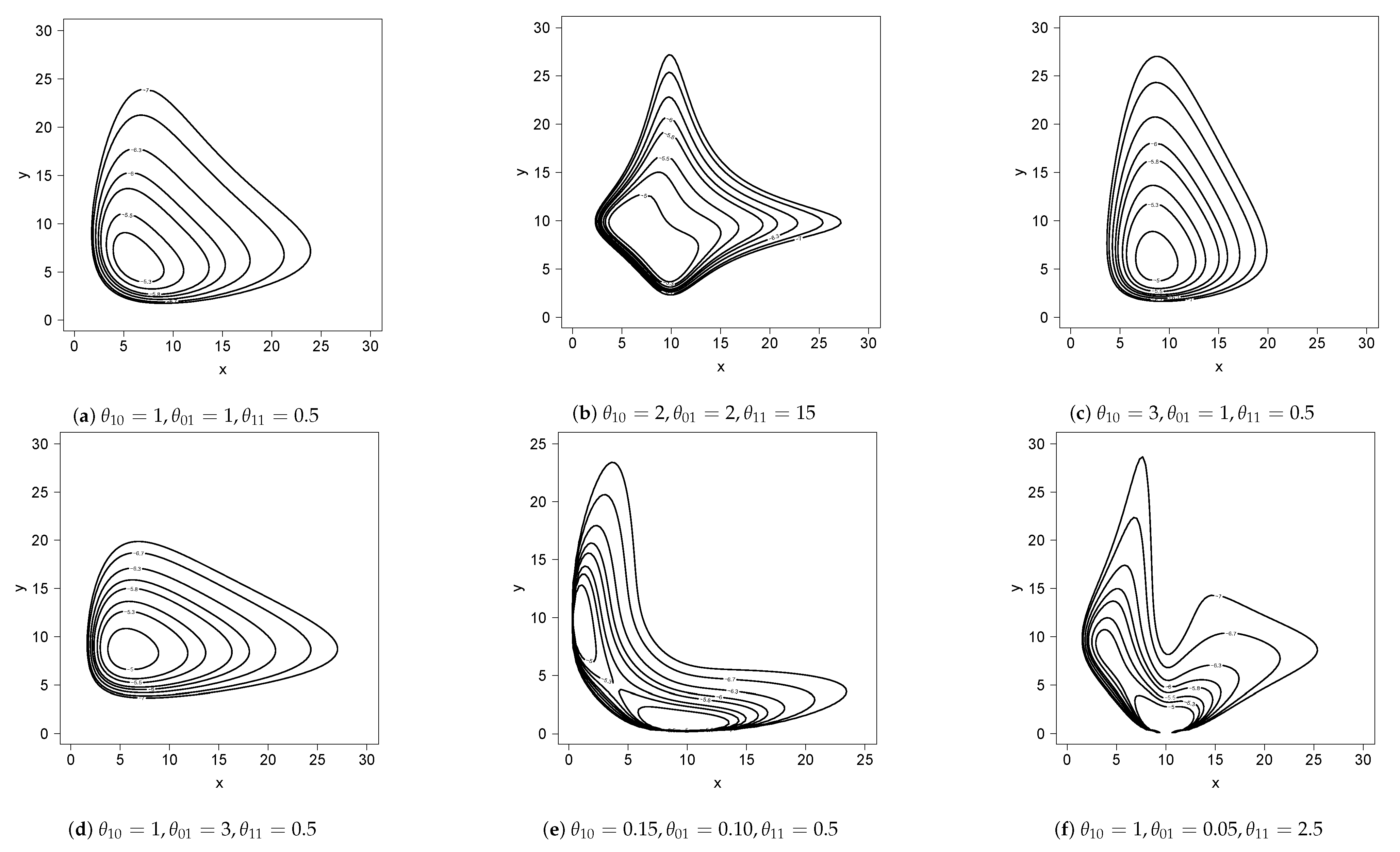
For added flexibility, we introduce scale parameters ${\beta }_X$ and ${\beta }_Y$ in this bivariate density. Thus, if $(X^{*},Y^{*})$ has density (2) and if we define $X={\beta }_X{X}^{*}$ and $Y={\beta }_Y{Y}^{*}$, then we can say that $(X,Y)$ has a general bivariate BS conditionals (BVBSC) distribution and we will write $(X,Y)\sim BVBSC({\beta }_X,{\beta }_Y,{\theta }_{10},{\theta }_{01},{\theta }_{11}).$ Figure 1 shows the scatterplot for the $BVBSC(10,10,{\theta }_{01},{\theta }_{10},{\theta }_{11})$ distribution with different values for the vector $({\theta }_{01},{\theta }_{10},{\theta }_{11})$. Note that the model can assume different shapes for the bivariate scatterplot depending on the values for the vector $({\theta }_{01},{\theta }_{10},{\theta }_{11})$.

2.1. Drawing Values from the Model

One advantage of the model is that both conditional distributions are specified in relatively simple forms. There is a well-known formula expressing a $BS(\beta ,\theta )$ variable denoted by U as a function of a standard normal variable Z, thus

$$U=\frac{\beta }{2}\left\{2+\frac{Z^2}{2\theta }+\frac{1}{\sqrt{2\theta }}Z\left[4+\frac{Z^2}{2\theta }\right]\right\}.$$

(6)

This can used whenever a BS draw is to be simulated.

There are two approaches that can be used to simulate draws from a general BS conditionals distribution. One approach involves simulation of a draw from the X marginal followed by use of the conditional density of Y given X to find the corresponding second coordinate of $(X,Y)$. For this approach, we wish to avoid drawing values directly from the marginal distribution because of possible problems in the computation of the normalizing constant. For this reason, to draw values from the marginal distribution of X, we propose the following steps based on the Metropolis–Hastings algorithm (Algorithm 1):

Algorithm 1 Metropolis–Hastings algorithm.

Set a start value $z_0$. A proposal can be selected by considering $z_0\sim BS(1,{\theta }_{10})$. Given a last value, say $z_{k-1}$, propose a new value as $z_k^{*}=x_{k-1}+ϵ$, where $ϵ\sim N(0,\tau )$. A possible choice for $\tau$ can be $\tau =1+{\theta }_{10}$, which corresponds to the variance of X for the independence case ${\theta }_{11}=0$. If $z_k>0$, set $z_k=z_k^{*}$ with probability $\pi =\frac{S\left(x_k\right)e^{-{\theta }_{10}T\left(z_k\right)}}{S\left(z_{k-1}\right)e^{-{\theta }_{10}T\left(z_{k-1}\right)}}\sqrt{\frac{{\theta }_{10}+{\theta }_{11}T\left(z_{k-1}\right)}{{\theta }_{10}+{\theta }_{11}T\left(z_k\right)}}$. Otherwise, set $z_k=z_{k-1}$. Repeat steps 2 and 3 as many times as necessary.

To eliminate the dependence among the drawn values, it is possible to consider a burn-in period and to thin the resulting series. Having drawn a final sample for X, say $x_1^{*},x_2^{*},\dots ,x_n^{*}$, we can simulate corresponding values for Y (using (5)) such that $y_i^{*}\sim BS(1,{\theta }_{01}+{\theta }_{11}T\left(x_i^{*}\right))$. Finally, the scale parameters can be introduced by setting $x_i={\beta }_X{x}_i^{*}$ and $y_i={\beta }_Y{y}_i^{*}$ for $i=1,\dots ,n$. The pairs $(x_1,y_1),(x_2,y_2),\dots ,(x_n,y_n)$ then constitute a simulated random sample from the model.

An alternative approach is one involving Gibbs sampler simulation utilizing the relative simplicity of the two corresponding conditional distributions (and the ease of drawing from univariate BS distributions). For it, we begin with an arbitrary value for X, say $x_0^{*}$. Then, we use the conditional distribution of Y given $X=x_0^{*}$ ( as in (5)) to simulate a corresponding $y_0^{*}$. Next, we generate a simulated value of X, say $x_1^{*}$, using the conditional distribution of X given $Y=y_0^{*}$ ( as in (4)), and continue in this fashion using (5) and (4) alternately. Use of burn-in and thinning is also recommended for this approach.

3. Estimation

Up to an additive constant, the log-likelihood function for $\psi =({\beta }_X,{\beta }_Y,{\theta }_{10},{\theta }_{01},{\theta }_{11})$ can be written as

$$\begin{array}{cc}\hfill \ell \left(\psi \right)& =\sum _{i=1}^n\left[logS\left(\frac{x_i}{{\beta }_X}\right)+logS\left(\frac{y_i}{{\beta }_Y}\right)-{\theta }_{01}T\left(\frac{y_i}{{\beta }_Y}\right)-\left({\theta }_{10}+{\theta }_{11}\right)T\left(\frac{x_i}{{\beta }_X}\right)\right]+nlogC,\hfill \end{array}$$

(7)

where

$$C^{-1}={\left[C({\theta }_{10},{\theta }_{01},{\theta }_{11})\right]}^{-1}={\int }_0^{\infty }\frac{S\left(u\right)e^{-{\theta }_{10}T\left(u\right)}}{\sqrt{{\theta }_{01}+{\theta }_{11}T\left(u\right)}}du.$$

However, the maximization of (7) can be challenging because of the need to repeatedly compute the quantity $C({\theta }_{10},{\theta }_{01},{\theta }_{11})$. For this reason, we recommend the implementation of the (conditional or) pseudo-likelihood approach. Besag [10] (see also Arnold and Strauss [11]) defined the pseudo-maximum likelihood estimator as that parameter vector that maximizes the pseudo-likelihood function, which for the bivariate case is given by

$$\begin{array}{cc}\hfill L\left(\psi \right)& =\prod _{i=1}^n{f}_{X_i\mid Y_i}(x_i\mid y_i,\psi )f_{Y_i\mid X_{i}i}(y_i\mid x_i,\psi ).\hfill \end{array}$$

For our proposed bivariate density, up to an additive constant, the log-pseudo-likelihood function is given by

$$\begin{array}{cc}\hfill \ell \left(\psi \right)& =\sum _{i=1}^n[logS\left(\frac{x_i}{{\beta }_X}\right)+logS\left(\frac{y_i}{{\beta }_Y}\right)-\frac{1}{2}log\left({\theta }_{10}+{\theta }_{11}T\left(\frac{y_i}{{\beta }_Y}\right)\right)-{\theta }_{10}-{\theta }_{01}\hfill \\ \hfill & -\frac{1}{2}log\left({\theta }_{01}+{\theta }_{11}T\left(\frac{x_i}{{\beta }_X}\right)\right)-{\theta }_{11}\left(T\left(\frac{x_i}{{\beta }_X}\right)+T\left(\frac{y_i}{{\beta }_Y}\right)\right)].\hfill \end{array}$$

(8)

The pseudo-likelihood estimates of the parameters are then obtained by numerically maximizing this expression.

4. Simulation Study

In this section, we present a brief simulation study in order to assess the recovery of parameter values based on the pseudo-maximum likelihood estimation discussed in Section 3. The data were drawn based on the first method described in Section 2.1, considering a burn-in period and a thinning of 1000 and 10, respectively. We consider ten different combinations for ${\beta }_1,{\beta }_2,{\theta }_{10},{\theta }_{01}$ and ${\theta }_{11}$. We also consider three sample sizes: 50, 100 and 200. For each combination of parameters and sample sizes, we consider 10,000 replicates. We present the average bias (AB), the mean of the standard errors (SE) based on the hessian matrix and the root of the mean squared error ($\sqrt{MSE}$) for those replicates. Results are presented in

Table 1. Simulation study to assess the recovery parameters for the BVBSC model under different scenarios and based on the pseudo-maximum likelihood estimation method.

True Value						$\mathit{n}=50$			$\mathit{n}=100$			$\mathit{n}=200$
${\mathit{\beta }}_{\mathbf{1}}$	${\mathit{\beta }}_{\mathbf{2}}$	${\mathit{\theta }}_{\mathbf{10}}$	${\mathit{\theta }}_{\mathbf{01}}$	${\mathit{\theta }}_{\mathbf{11}}$	est.	AB	SE	$\sqrt{\mathit{MSE}}$	AB	SE	$\sqrt{\mathit{MSE}}$	AB	SE	$\sqrt{\mathit{MSE}}$
1	1	0.5	0.5	0.5	${\widehat{\beta }}_1$	0.006	0.092	0.129	0.002	0.065	0.087	0.000	0.046	0.061
					${\widehat{\beta }}_2$	0.007	0.092	0.114	0.002	0.065	0.077	0.002	0.046	0.053
					${\widehat{\theta }}_{10}$	0.036	0.159	0.198	0.023	0.108	0.137	0.011	0.074	0.095
					${\widehat{\theta }}_{01}$	0.017	0.154	0.174	0.011	0.106	0.116	0.005	0.073	0.079
					${\widehat{\theta }}_{11}$	0.186	0.275	0.468	0.082	0.174	0.267	0.038	0.116	0.168
				2	${\widehat{\beta }}_1$	0.001	0.064	0.087	0.000	0.045	0.060	0.000	0.032	0.043
					${\widehat{\beta }}_2$	0.002	0.064	0.085	0.002	0.045	0.058	0.001	0.032	0.041
					${\widehat{\theta }}_{10}$	0.048	0.185	0.226	0.024	0.124	0.150	0.013	0.085	0.107
					${\widehat{\theta }}_{01}$	0.023	0.178	0.195	0.011	0.121	0.128	0.006	0.084	0.086
					${\widehat{\theta }}_{11}$	0.463	0.702	1.131	0.214	0.452	0.668	0.109	0.307	0.433
			2	0.5	${\widehat{\beta }}_1$	0.010	0.112	0.161	0.003	0.080	0.113	0.002	0.056	0.079
					${\widehat{\beta }}_2$	0.003	0.060	0.068	0.001	0.043	0.046	0.001	0.031	0.033
					${\widehat{\theta }}_{10}$	0.032	0.139	0.173	0.017	0.094	0.121	0.012	0.065	0.088
					${\widehat{\theta }}_{01}$	0.041	0.536	0.591	0.023	0.369	0.405	0.015	0.258	0.281
					${\widehat{\theta }}_{11}$	0.382	0.521	0.965	0.160	0.329	0.528	0.072	0.223	0.330
				2	${\widehat{\beta }}_1$	0.005	0.092	0.128	0.002	0.065	0.087	0.001	0.046	0.061
					${\widehat{\beta }}_2$	0.001	0.049	0.058	0.001	0.035	0.040	0.001	0.025	0.028
					${\widehat{\theta }}_{10}$	0.040	0.160	0.205	0.023	0.108	0.135	0.013	0.074	0.096
					${\widehat{\theta }}_{01}$	0.076	0.617	0.687	0.036	0.420	0.460	0.024	0.293	0.313
					${\widehat{\theta }}_{11}$	0.710	1.094	1.848	0.314	0.694	1.041	0.152	0.464	0.686
		2	0.5	0.5	${\widehat{\beta }}_1$	0.002	0.060	0.071	0.001	0.043	0.048	0.001	0.031	0.034
					${\widehat{\beta }}_2$	0.009	0.113	0.131	0.003	0.080	0.087	0.001	0.056	0.060
					${\widehat{\theta }}_{10}$	0.046	0.538	0.607	0.024	0.370	0.419	0.014	0.258	0.291
					${\widehat{\theta }}_{01}$	0.007	0.134	0.147	0.004	0.092	0.100	0.005	0.065	0.071
					${\widehat{\theta }}_{11}$	0.385	0.515	0.939	0.173	0.329	0.532	0.069	0.220	0.326
		2	0.5	2	${\widehat{\beta }}_1$	0.001	0.048	0.059	0.001	0.034	0.042	0.000	0.024	0.029
					${\widehat{\beta }}_2$	0.007	0.092	0.113	0.003	0.065	0.076	0.001	0.046	0.053
					${\widehat{\theta }}_{10}$	0.070	0.616	0.697	0.036	0.420	0.475	0.014	0.292	0.320
					${\widehat{\theta }}_{01}$	0.015	0.154	0.174	0.009	0.105	0.115	0.004	0.073	0.077
					${\widehat{\theta }}_{11}$	0.763	1.093	1.842	0.331	0.690	1.065	0.166	0.462	0.673
			2	0.5	${\widehat{\beta }}_1$	0.003	0.065	0.076	0.002	0.047	0.052	0.001	0.033	0.036
					${\widehat{\beta }}_2$	0.004	0.065	0.072	0.002	0.047	0.049	0.001	0.033	0.034
					${\widehat{\theta }}_{10}$	−0.015	0.483	0.534	0.009	0.335	0.361	−0.001	0.234	0.255
					${\widehat{\theta }}_{01}$	−0.020	0.483	0.513	0.002	0.334	0.354	−0.002	0.234	0.246
					${\widehat{\theta }}_{11}$	1.254	1.238	2.655	0.562	0.747	1.375	0.254	0.500	0.810
				2	${\widehat{\beta }}_1$	0.002	0.060	0.071	0.001	0.043	0.049	0.001	0.031	0.034
					${\widehat{\beta }}_2$	0.002	0.060	0.068	0.001	0.043	0.047	0.000	0.031	0.032
					${\widehat{\theta }}_{10}$	0.047	0.537	0.611	0.017	0.369	0.405	0.016	0.258	0.288
					${\widehat{\theta }}_{01}$	0.030	0.532	0.593	0.011	0.367	0.397	0.017	0.258	0.281
					${\widehat{\theta }}_{11}$	1.504	2.043	3.769	0.684	1.308	2.098	0.301	0.885	1.321
2	5	0.5	0.5	0.5	${\widehat{\beta }}_1$	0.009	0.183	0.253	−0.005	0.129	0.170	0.001	0.092	0.123
					${\widehat{\beta }}_2$	0.041	0.462	0.566	0.001	0.325	0.385	0.009	0.231	0.265
					${\widehat{\theta }}_{10}$	0.042	0.160	0.204	0.022	0.108	0.134	0.013	0.074	0.096
					${\widehat{\theta }}_{01}$	0.019	0.155	0.173	0.009	0.105	0.115	0.006	0.073	0.080
					${\widehat{\theta }}_{11}$	0.186	0.277	0.465	0.082	0.174	0.265	0.037	0.116	0.168
0.25	0.75	0.5	0.5	2	${\widehat{\beta }}_1$	0.001	0.016	0.028	0.000	0.011	0.015	0.002	0.008	0.011
					${\widehat{\beta }}_2$	0.007	0.049	0.135	0.002	0.034	0.043	0.002	0.024	0.096
					${\widehat{\theta }}_{10}$	0.034	0.180	0.235	0.027	0.124	0.154	0.006	0.084	0.113
					${\widehat{\theta }}_{01}$	0.025	0.179	0.198	0.011	0.121	0.127	0.023	0.087	0.094
					${\widehat{\theta }}_{11}$	0.449	0.695	1.136	0.215	0.453	0.674	0.110	0.308	0.450

. It can be observed that accurate estimation of the dependence parameter ${\theta }_{11}$ appears to require a quite large sample size. This is not unexpected since dependence parameters are routinely more elusive in conditionally specified models. Simulation and applications codes were written in the R programming language R [12].

5. Applications

In this section, we present two applications to compare our proposal with two other bivariate BS distributions that have been considered in the literature. The parameter estimation was performed based on the pseudo-maximum likelihood (ML) estimation method for the BVBSC model and the traditional ML estimation method for the other models. Both data sets (Section 5.1 and Section 5.2) have been used in many papers, particularly in univariate distributional settings.

Regarding the first application, the variable Neodymium was used in Reyes et al. [3] and Bourguignon and Gallardo [13] in a univariate context. For the second application, Arellano-Valle et al. [14] used the variable weight, also in a univariate context.

5.1. Minerals Data Set

This data set corresponds to lanthanum and neodymium measurements collected by the Department of Mines of the University of Atacama, Chile, representing 86 samples of both minerals (see Supplementary Materials). Some descriptive statistics for this data set are presented in

Table 2. Descriptive measure for minerals data set.

Variable	Min.	Max.	Median	Mean	s.d.	Skewness	Kurtosis
lanthanum	1	331	37	52.24	70.47	2.65	8.85
neodymium	4	219	28.5	35.02	34.23	3.65	18.22

.

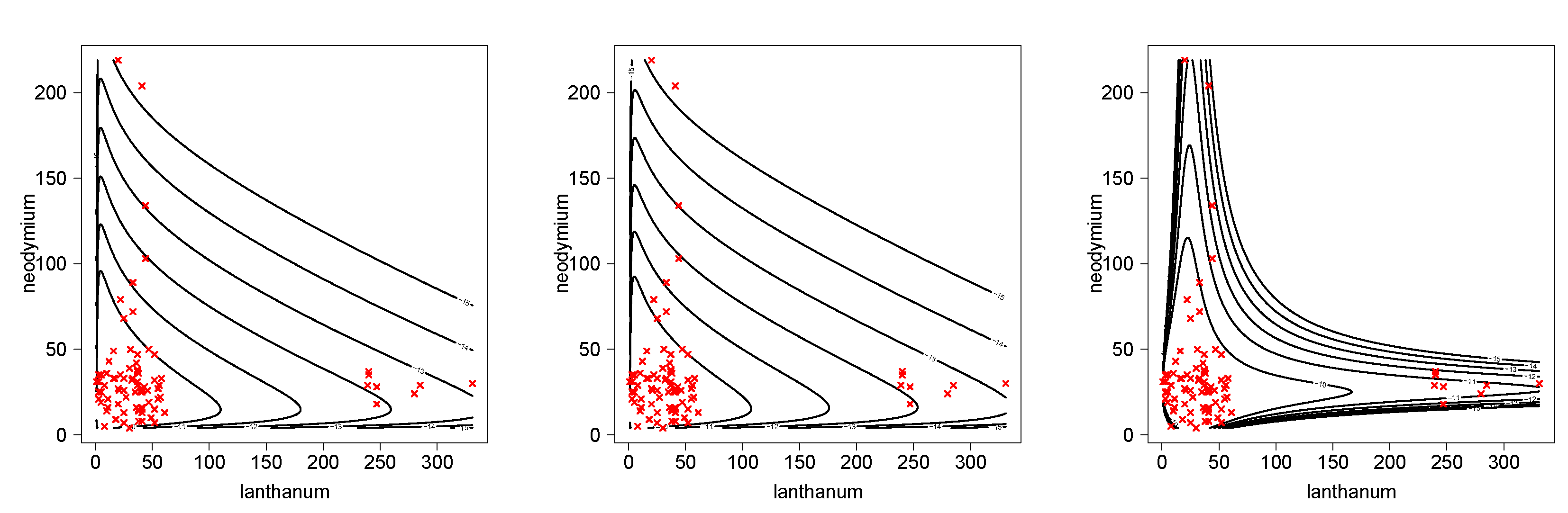
We fitted the bivariate BS (BVBS) discussed in Kundu et al. [15] and the bivariate BS (BVBS2) proposed by Lemonte et al. [16]. The formulas for the densities corresponding to these models are displayed in the Appendix A. Results are presented in

Table 3. Estimates for different bivariate BS-type models in the minerals data set based on the pseudo-ML estimation (BVBSC) model and the ML estimation (BVBS and BVBS2 models) and standard errors in brackets.

Parameter	BVBS	BVBS2	BVBSC
${\alpha }_1$	1.4139 (0.1080)	1.4144 (0.1080)	-
${\alpha }_2$	0.7577 (0.0578)	0.7576 (0.0578)	-
${\beta }_1$	25.2075 (3.0529)	25.2044 (3.0525)	25.7728 (1.9685)
${\beta }_2$	27.2319 (2.0786)	27.1446 (2.0719)	27.3922 (2.0886)
$\rho$	0.0110 (0.0012)	-	-
$\lambda$	-	0.0723 (0.0078)	-
${\theta }_{10}$	-	-	0.1448 (0.0175)
${\theta }_{01}$	-	-	0.5193 (0.0396)
${\theta }_{11}$	-	-	0.9133 (0.0989)
AIC	1623.33	1623.29	1568.93
BIC	1635.60	1635.56	1581.20

. In order to compare the models, the AIC (see Akaike [17]) and BIC (see Schwarz [18]) criteria are considered. The conditionally specified model appears to be markedly superior to the other two bivariate BS models. It should be remarked, however, that, since the conditionally specified model fails to have BS marginals, it might be difficult to convince a scientist to use it if they feel that there are valid scientific reasons to believe that BS marginals are appropriate. Figure 2 shows the better fit for the mineral data set of the BVBSC when compared with the BVBS and BVBS2 models.

5.2. Australian Athletes Data Set

These data are related to measurements of 202 Australian athletes found in Cook and Weisberg [8]. For each athlete various characteristics of the blood were determined together with data regarding the sport, body size and gender of the athlete. In particular, we consider two measurements, the Body fat percentage (Bfat) and the weight in kg. Some descriptive statistics for this data set are presented in

Table 4. Descriptive measure for athletes data set

Variable	Min.	Max.	Median	Mean	s.d.	Skewness	Kurtosis
Bfat	5.63	35.52	11.65	13.51	6.19	0.76	2.83
Weight	37.80	66.53	74.40	75.01	13.93	0.24	3.39

.

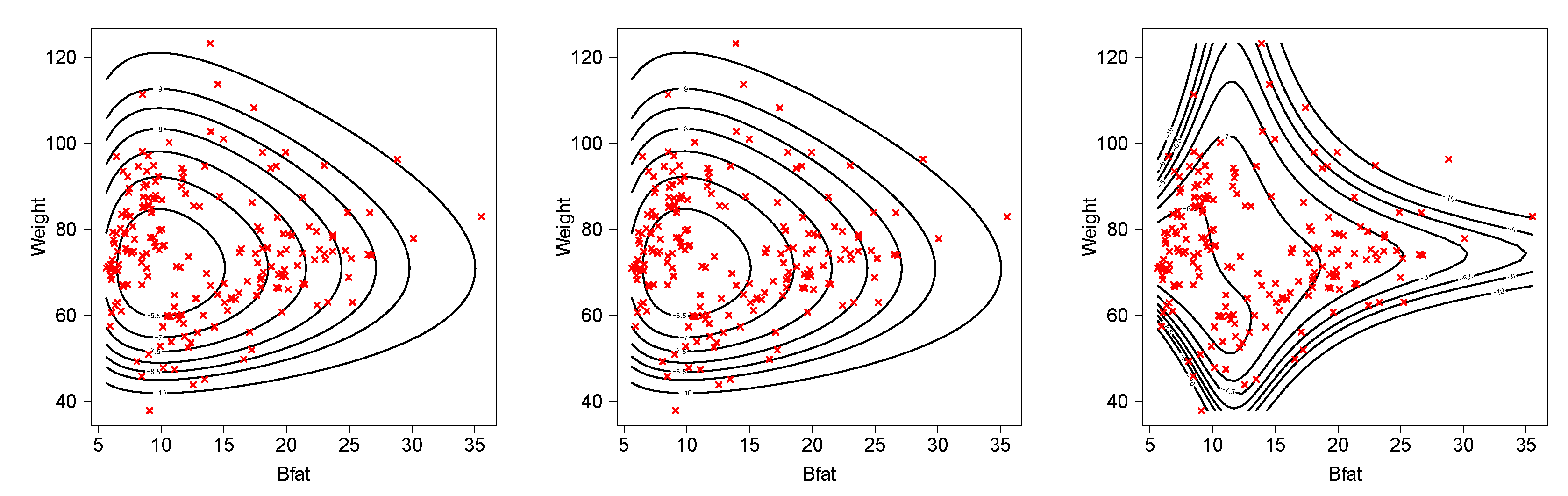
We fitted the same three bivariate BS models to these data as were fitted in Section 5.1. Results are presented in

Table 5. Estimates for different bivariate BS-type models in the athlete data set based on the pseudo-ML estimation (BVBSC) model and the ML estimation (BVBS and BVBS2 models) and standard errors in brackets.

Parameter	BVBS	BVBS2	BVBSC
${\alpha }_1$	0.4583 (0.0228)	0.4583 (0.0228)	-
${\alpha }_2$	0.1912 (0.0095)	0.1912 (0.0095)	-
${\beta }_1$	12.2255 (0.3838)	12.2245 (0.3838)	11.8503 (0.5896)
${\beta }_2$	73.6622 (0.9862)	73.6632 (0.9862)	74.5503 (3.7090)
$\rho$	−0.0040 (0.0003)	-	-
$\lambda$	-	−0.0097 (0.0007)	-
${\theta }_{10}$	-	-	1.5367 (0.0482)
${\theta }_{01}$	-	-	7.3707 (0.0987)
${\theta }_{11}$	-	-	50.3277 (3.5410)
AIC	2908.67	2908.67	2856.04
BIC	2925.21	2925.21	2872.58

. Again, the conditionally specified model appears to be superior to the other two bivariate BS models. Figure 3 shows the better fit for the athlete data set of the BVBSC when compared with the BVBS and BVBS2 models.

6. Discussion

The BS density has been utilized in a wide range of scientific and economic settings as a suitable model for non-negative data. As was remarked in the Introduction, its genesis was in the context of fatigue life distributions, but its relative simplicity has led to successful application in many other fields. There are, of course, many ways in which we might seek to develop suitable bivariate BS models. One approach involves the use of copulas to link BS marginals. An example of this approach is the Kundu et al. [15] model, which can be viewed as utilizing a classical bivariate normal copula. The model proposed by Lemonte et al. [16] involves marginal transformations of a well-known bivariate skew normal model. The proposal, in the current paper, of using a conditionally specified model does have the drawback of not having BS marginals, but, as has been demonstrated, it fares well, when compared to the two models described above, in terms of fitting the data sets discussed here.

The field is, of course, open for the development of alternative bivariate BS distributions distinct from those discussed here. It must be kept in mind that we cannot expect to find an overall best bivariate BS model. Some will be good for certain kinds of data, while others will be better for different data configurations.

References

- Leiva, V. The Birnbaum-Saunders Distribution; Academic Press: New York, NY, USA, 2016. [Google Scholar]
- Balakrishnan, N.; Kundu, D. Birnbaum-Saunders distribution: A review of models, analysis, and applications. Appl. Stoch. Model. Bus. Ind. 2019, 35, 4–49. [Google Scholar] [CrossRef] [Green Version]
- Reyes, J.; Barranco-Chamorro, I.; Gallardo, D.I.; Gómez, H.W. Generalized Modified Slash Birnbaum-Saunders Distribution. Symmetry 2018, 10, 724. [Google Scholar] [CrossRef] [Green Version]
- Martínez-Flérez, G.; Barranco-Chamorro, I.; Bolfarine, H.; Gómez, H.W. Flexible Birnbaum–Saunders Distribution. Symmetry 2018, 11, 1305. [Google Scholar] [CrossRef] [Green Version]
- Gómez-Déniz, E.; Gómez, L. The Rayleigh Birnbaum Saunders Distribution: A General Fading Model. Symmetry 2020, 12, 389. [Google Scholar] [CrossRef] [Green Version]
- Mazucheli, J.; Leiva, V.; Alves, B.; Menezes, A.F.B. A New Quantile Regression for Modeling Bounded Data under a Unit Birnbaum–Saunders Distribution with Applications in Medicine and Politics. Symmetry 2021, 13, 682. [Google Scholar] [CrossRef]
- Arnold, B.C.; Castillo, E.; Sarabia, J.M. Conditional Specification of Statistical Models; Springer Series in Statistics; Springer: Berlin/Heidelberg, Germany, 1999. [Google Scholar]
- Cook, R.D.; Weisberg, S. An Introduction to Regression Graphics; John Wiley& Sons Inc.: New York, NY, USA, 1994. [Google Scholar]
- Arnold, B.C.; Strauss, D.J. Bivariate distributions with conditionals in prescribed exponential families. J. R. Stat. Soc. Ser. B 1991, 53, 365–375. [Google Scholar]
- Besag, J. Statistical Analysis of Non-Lattice Data. J. R. Stat. Soc. Ser. D 1975, 24, 179–195. [Google Scholar] [CrossRef] [Green Version]
- Arnold, B.C.; Strauss, D.J. Pseudolikelihood estimation: Some examples. Sankhya Ser. B 1991, 53, 233–243. [Google Scholar]
- R Development Core Team. A Language and Environment for Statistical Computing; R Foundation for Statistical Computing: Vienna, Austria, 2019. [Google Scholar]
- Arellano-Valle, R.B.; Castro, L.M.; Genton, M.G.; Gómez, H.W. Bayesian Inference for Shape Mixtures of Skewed Distributions, with Application to Regression Analysis. Bayesian Anal. 2008, 3, 513–540. [Google Scholar] [CrossRef]
- Bourguignon, M.; Gallardo, D.I. Reparameterized inverse gamma regression models with varying precision. Statistica Neerlandica 2020, 74, 611–627. [Google Scholar] [CrossRef]
- Kundu, D.; Balakrishnan, N.; Jamalizadeh, A. Bivariate Birnbaum-Saunders distribution and associated inference. J. Multivar. Anal. 2010, 101, 113–125. [Google Scholar] [CrossRef] [Green Version]
- Lemonte, A.J.; Martínez-Florez, G.; Moreno-Arenas, G. Multivariate Birnbaum-Saunders distribution: Properties and associated inference. J. Stat. Comput. Simul. 2015, 85, 374–392. [Google Scholar] [CrossRef]
- Akaike, H. A new look at the statistical model identification. IEEE Trans. Autom. Control. 1974, 19, 716–723. [Google Scholar] [CrossRef]
- Schwarz, G. Estimating the dimension of a model. Ann Stat. 1978, 6, 461–464. [Google Scholar] [CrossRef]
Figure 1.
Scatterplot for distribution with different values for .
Figure 2.
Scatterplot of minerals data and contour level of the fitted models. BVBS (left panel), BVBS2 (center panel) and BVBSC (right panel).
Figure 3.
Scatterplot of athlete data and contour level of the fitted models. BVBS (left panel), BVBS2 (center panel) and BVBSC (right panel).